Expected Accuracy in a Measurement of the CKM Angle ฮฑ๐›ผ\alpha Using a Dalitz Plot Analysis of B0โ†’ฯโ€‹ฯ€โ†’superscript๐ต0๐œŒ๐œ‹\boldmath B^{0}\to\rho\pi Decays in the BTeV Project

K.E.ย Shestermanov A.Nย Vasiliev J.ย Butler A.A.ย Derevschikov P.Kasper V.V.ย Kiselev V.I.ย Kravtsov Y.ย Kubota R.Kutschke Y.A.ย Matulenko N.G.ย Minaev V.V.ย Mochalov D.A.ย Morozov L.V.ย Nogach M.ย Rovere A.V.ย Ryazantsev P.A.ย Semenov S.ย Stone A.V.ย Uzunian J.ย Yarba Institute for High Energy Physics, Protvino 142281, Russia Fermilab, Batavia, IL 60510, U.S.A. University of Minnesota, Minneapolis, MN 55455, U.S.A. Syracuse University, Syracuse, NY 13244-1130, U.S.A. Istituto Nazionale di Fisica Nucleare - Sezione di Milano, Milano I-20133, Italy
Abstract

A precise measurement of the angle ฮฑ๐›ผ\alpha in the CKM triangle is very important for a complete test of Standard Model. A theoretically clean method to extract ฮฑ๐›ผ\alpha is provided by Bโ†’0ฯฯ€{}^{0}\to\rho\pi decays. Monte Carlo simulations to obtain the BTeV reconstruction efficiency and to estimate the signal to background ratio for these decays were performed. Finally the time-dependent Dalitz plot analysis, using the isospin amplitude formalism for tree and penguin contributions, was carried out. It was shown that in one year of data taking BTeV could achieve an accuracy on ฮฑ๐›ผ\alpha better than 5โˆ˜.

, โ€ โ€ thanks: untimely deceased , โ€ โ€ thanks: corresponding author, email: Alexander.Vasiliev@ihep.ru , , , , , , , , , , , , , , , , ,

1 Introduction

The Standard Model (SM)ย [1] which incorporates the quark mixing Cabbibo-Kabayashi-Maskawa (CKM) mechanismย [2] has been increasingly successful, supported with many precise experimental results. This strongly indicates that, at low energies, the SM is the effective description of Nature. However, there are reasons to believe that there exists physics beyond the SM. For example, from the astrophysical point of view, it is a serious problem that the matter-antimatter asymmetry in the Universe can not be explained solely from the CP violation in the SM, which originates from quark flavor mixing. This observation, together with others, leads one to believe that there is a new physics, most likely, at the TeV energy scale. One of the critical measurements to test the SM or to obtain strong indications of new physics are precisie measurements of the angles in the Unitary Triangles (UT), which are of non-zero area if CP violation exists.

A unique program that would have allowed one to challenge the SM explanation of CP violation, mixing and rare decays in the b๐‘b and c๐‘c quark system was proposed by the BTeV project [4] at the Tevatron at Fermilab. The design of BTeV exceled in several crucial areas including: triggering on decays with purely hadronic final states, charged particle identification, excellent electromagnetic calorimetry and excellent proper time resolution. Exploiting the large number of b๐‘bโ€™s and c๐‘cโ€™s produced at the Tevatron collider, the experiment would have provided precise measurements of SM parameters and an exhaustive search for physics beyond the SM. The complete physics objectives of BTeV included measuring the CP violating angles ฮฑ๐›ผ\alpha, ฮฒ๐›ฝ\beta, and ฮณ๐›พ\gamma of the UT. In particular, the measurement of ฮฑ๐›ผ\alpha is difficult due to small overall rates and because the gluonic penguin rates are of the same order as the tree rates, causing well known difficulties in extracting the weak phase angle. Quinn and Snyderย [5] have suggested a theoretically clean method to extract ฮฑ๐›ผ\alpha from decays of the type B0โ†’ฯโ€‹ฯ€โ†’superscript๐ต0๐œŒ๐œ‹B^{0}\rightarrow\rho\pi. The final state of these decays is not a CP eigenstate, which results in the need of a Dalitz plot analysis. We focus on the measurement of ฮฑ๐›ผ\alpha, via collecting a large sample of B0โ†’(ฯโ€‹ฯ€)0โ†’superscript๐ต0superscript๐œŒ๐œ‹0B^{0}\rightarrow(\rho\pi)^{0} decays. Direct measurements from the B-factories demonstrate that the average hโ€‹hโ„Žโ„Žhh decays (where h=(ฯ,ฯ€)โ„Ž๐œŒ๐œ‹h=(\rho,\pi)) is known to a precision of Oโ€‹(10o)๐‘‚superscript10๐‘œO(10^{o})ย [3], with the use of isospin. In this paper we demonstrate that BTeV could have done the measurement with a much better precision.

The paper is organized as follows. Section 2 provides brief introduction of the CKM matrix. In section 3 we give a general overview of the BTeV project. In sections 4 and 5, respectively, we report on the expected reconstruction efficiencies and the Signal/Background ratio of the B0โ†’(ฯโ€‹ฯ€)0โ†’superscript๐ต0superscript๐œŒ๐œ‹0B^{0}\rightarrow(\rho\pi)^{0} decays in BTeV. Section 6 covers the phenomenological formalism of B0โ†’(ฯโ€‹ฯ€)0โ†’superscript๐ต0superscript๐œŒ๐œ‹0B^{0}\rightarrow(\rho\pi)^{0} decays. In section 7 we describe results of the time-dependent Dalitz plot analysis of the simulated B0โ†’(ฯโ€‹ฯ€)0โ†’superscript๐ต0superscript๐œŒ๐œ‹0B^{0}\rightarrow(\rho\pi)^{0} decays in BTeV.

2 The CKM Matrix and the Angle ฮฑ๐›ผ\boldmath\alpha

In the SM there are three generations of leptons and quarks. The physical point-like particles that have both strong and electroweak interactions, the quark, are mixtures of weak eigenstates, described by a 3x3 unitary matrix, called the Cabibbo-Kobayashi-Maskawaย (CKM) matrix [2],

(dโ€ฒsโ€ฒbโ€ฒ)=(Vuโ€‹dVuโ€‹sVuโ€‹bVcโ€‹dVcโ€‹sVcโ€‹bVtโ€‹dVtโ€‹sVtโ€‹b)โ€‹(dsb)superscript๐‘‘โ€ฒsuperscript๐‘ โ€ฒsuperscript๐‘โ€ฒsubscript๐‘‰๐‘ข๐‘‘subscript๐‘‰๐‘ข๐‘ subscript๐‘‰๐‘ข๐‘subscript๐‘‰๐‘๐‘‘subscript๐‘‰๐‘๐‘ subscript๐‘‰๐‘๐‘subscript๐‘‰๐‘ก๐‘‘subscript๐‘‰๐‘ก๐‘ subscript๐‘‰๐‘ก๐‘๐‘‘๐‘ ๐‘\left(\begin{array}[]{c}d^{\prime}\\ s^{\prime}\\ b^{\prime}\\ \end{array}\right)=\left(\begin{array}[]{ccc}V_{ud}&V_{us}&V_{ub}\\ V_{cd}&V_{cs}&V_{cb}\\ V_{td}&V_{ts}&V_{tb}\end{array}\right)\left(\begin{array}[]{c}d\\ s\\ b\\ \end{array}\right) (1)

The unprimed states are the mass eigenstates, while the primed states denote the weak eigenstates. The Viโ€‹jsubscript๐‘‰๐‘–๐‘—V_{ij}โ€™s are complex numbers that can be expressed in terms of four independent real quantities. These numbers are fundamental constants of Nature that need to be determined from experiment. In the Wolfenstein approximation the matrix is written as [6]

VCโ€‹Kโ€‹M=(1โˆ’ฮป2/2ฮปAโ€‹ฮป3โ€‹(ฯโˆ’iโ€‹ฮทโ€‹(1โˆ’ฮป2/2))โˆ’ฮป1โˆ’ฮป2/2โˆ’iโ€‹ฮทโ€‹A2โ€‹ฮป4Aโ€‹ฮป2โ€‹(1+iโ€‹ฮทโ€‹ฮป2)Aโ€‹ฮป3โ€‹(1โˆ’ฯโˆ’iโ€‹ฮท)โˆ’Aโ€‹ฮป21)subscript๐‘‰๐ถ๐พ๐‘€1superscript๐œ†22๐œ†๐ดsuperscript๐œ†3๐œŒ๐‘–๐œ‚1superscript๐œ†22๐œ†1superscript๐œ†22๐‘–๐œ‚superscript๐ด2superscript๐œ†4๐ดsuperscript๐œ†21๐‘–๐œ‚superscript๐œ†2๐ดsuperscript๐œ†31๐œŒ๐‘–๐œ‚๐ดsuperscript๐œ†21V_{CKM}=\left(\begin{array}[]{ccc}1-\lambda^{2}/2&\lambda&A\lambda^{3}(\rho-i\eta(1-\lambda^{2}/2))\\ -\lambda&1-\lambda^{2}/2-i\eta A^{2}\lambda^{4}&A\lambda^{2}(1+i\eta\lambda^{2})\\ A\lambda^{3}(1-\rho-i\eta)&-A\lambda^{2}&1\end{array}\right) (2)

where (ฮป๐œ†\lambda, A๐ดA, ฯ๐œŒ\rho, ฮท๐œ‚\eta) are four mixing parameters with ฮป=|Vuโ€‹s|โ‰ˆ0.22๐œ†subscript๐‘‰๐‘ข๐‘ 0.22\lambda=|V_{us}|\approx 0.22, Aโ‰ˆ0.8๐ด0.8A\approx 0.8 (measured using semileptonic s๐‘ s and b๐‘b decays [7]), and ฮท๐œ‚\eta represents the CP violating phase. This expression is accurate to order ฮป3superscript๐œ†3\lambda^{3} in the real part and ฮป5superscript๐œ†5\lambda^{5} in the imaginary part. It is necessary to express the matrix to this order to have a complete formulation of the physics we wish to pursue.

The unitarity of the CKM matrix leads to various relations among the matrix elements

Vuโ€‹dโ€‹Vuโ€‹sโˆ—+Vcโ€‹dโ€‹Vcโ€‹sโˆ—+Vtโ€‹dโ€‹Vtโ€‹sโˆ—=0subscript๐‘‰๐‘ข๐‘‘superscriptsubscript๐‘‰๐‘ข๐‘ subscript๐‘‰๐‘๐‘‘superscriptsubscript๐‘‰๐‘๐‘ subscript๐‘‰๐‘ก๐‘‘superscriptsubscript๐‘‰๐‘ก๐‘ 0V_{ud}V_{us}^{*}+V_{cd}V_{cs}^{*}+V_{td}V_{ts}^{*}=0 (3)
Vuโ€‹sโ€‹Vuโ€‹bโˆ—+Vcโ€‹sโ€‹Vcโ€‹bโˆ—+Vtโ€‹sโ€‹Vtโ€‹bโˆ—=0subscript๐‘‰๐‘ข๐‘ superscriptsubscript๐‘‰๐‘ข๐‘subscript๐‘‰๐‘๐‘ superscriptsubscript๐‘‰๐‘๐‘subscript๐‘‰๐‘ก๐‘ superscriptsubscript๐‘‰๐‘ก๐‘0V_{us}V_{ub}^{*}+V_{cs}V_{cb}^{*}+V_{ts}V_{tb}^{*}=0 (4)
Vuโ€‹bโ€‹Vuโ€‹dโˆ—+Vcโ€‹bโ€‹Vcโ€‹dโˆ—+Vtโ€‹bโ€‹Vtโ€‹dโˆ—=0subscript๐‘‰๐‘ข๐‘superscriptsubscript๐‘‰๐‘ข๐‘‘subscript๐‘‰๐‘๐‘superscriptsubscript๐‘‰๐‘๐‘‘subscript๐‘‰๐‘ก๐‘superscriptsubscript๐‘‰๐‘ก๐‘‘0V_{ub}V_{ud}^{*}+V_{cb}V_{cd}^{*}+V_{tb}V_{td}^{*}=0 (5)

that can be geometrically represented in the complex plane as triangles. These are โ€œunitary trianglesโ€, though the term โ€œunitary triangleโ€ is usually reserved only for the bd triangle in (5) where the angles are all thought to be relatively large. This CKM triangle is depicted in Figureย 1. It shows the angles ฮฑ,ฮฒ๐›ผ๐›ฝ\alpha,~{}\beta, and ฮณ๐›พ\gamma. These angles are defined as

ฮฑ=aโ€‹rโ€‹gโ€‹[โˆ’Vtโ€‹dโ€‹Vtโ€‹bโˆ—Vuโ€‹dโ€‹Vuโ€‹bโˆ—],ฮฒ=aโ€‹rโ€‹gโ€‹[โˆ’Vcโ€‹dโ€‹Vcโ€‹bโˆ—Vtโ€‹dโ€‹Vtโ€‹bโˆ—],ฮณ=aโ€‹rโ€‹gโ€‹[โˆ’Vuโ€‹dโ€‹Vuโ€‹bโˆ—Vcโ€‹dโ€‹Vcโ€‹bโˆ—]formulae-sequence๐›ผ๐‘Ž๐‘Ÿ๐‘”delimited-[]subscript๐‘‰๐‘ก๐‘‘subscriptsuperscript๐‘‰๐‘ก๐‘subscript๐‘‰๐‘ข๐‘‘subscriptsuperscript๐‘‰๐‘ข๐‘formulae-sequence๐›ฝ๐‘Ž๐‘Ÿ๐‘”delimited-[]subscript๐‘‰๐‘๐‘‘subscriptsuperscript๐‘‰๐‘๐‘subscript๐‘‰๐‘ก๐‘‘subscriptsuperscript๐‘‰๐‘ก๐‘๐›พ๐‘Ž๐‘Ÿ๐‘”delimited-[]subscript๐‘‰๐‘ข๐‘‘subscriptsuperscript๐‘‰๐‘ข๐‘subscript๐‘‰๐‘๐‘‘subscriptsuperscript๐‘‰๐‘๐‘\displaystyle\alpha=arg\left[-{V_{td}V^{*}_{tb}\over V_{ud}V^{*}_{ub}}\right],~{}~{}~{}\beta=arg\left[-{V_{cd}V^{*}_{cb}\over V_{td}V^{*}_{tb}}\right],~{}~{}~{}\gamma=arg\left[-{{V_{ud}V^{*}_{ub}}\over{V_{cd}V^{*}_{cb}}}\right] (6)

and can be determined by measuring CP violation in B๐ตB decays.

Refer to caption

Figure 1: Unitary Triangle.

They can roughly be divided in two classes :

  • โ€ข

    decays that are expected to have relatively small direct CP violation and hence are particularly interesting for extracting CKM parameters from interference of decays with and without mixing.

  • โ€ข

    decays in which direct CP violation could be significant and therefore that can not be cleanly interpreted in terms of CKM phases.

B๐ตB decays used to extract ฮฒ๐›ฝ\beta belong to the first group, whereas decays that have been considered to measure ฮฑ๐›ผ\alpha belong to the second one.

The primary source for measurements of sin(2โ€‹ฮฒ2๐›ฝ2\beta) are the decays of the type bโ†’cโ€‹cยฏโ€‹sโ†’๐‘๐‘ยฏ๐‘๐‘ b\to c\overline{c}s. The most statistically significant measurements of CP violation in the B๐ตB system were made by BABARย [9] and BELLEย [10], resulting in the average value of sin(2โ€‹ฮฒ2๐›ฝ2\beta)=0.725ยฑplus-or-minus\pm0.037ย [11].

Measuring ฮฑ๐›ผ\alpha is more difficult than measuring ฮฒ๐›ฝ\beta in several respects. First of all, the decay amplitudes are modulated by Vuโ€‹bsubscript๐‘‰๐‘ข๐‘V_{ub} rather than Vcโ€‹bsubscript๐‘‰๐‘๐‘V_{cb} making the overall rates small, of the order of 10โˆ’5superscript10510^{-5} to 10โˆ’6superscript10610^{-6}. Secondly, the gluonic penguin rates are of the same order as the trees causing large theoretical uncertainties in cleanly extracting ฮฑ๐›ผ\alpha from asymmetry measurements, alone.

The decay B0โ†’ฯ€+โ€‹ฯ€โˆ’โ†’superscript๐ต0superscript๐œ‹superscript๐œ‹B^{0}\rightarrow\pi^{+}\pi^{-} has been proposed as a way to measure sin(2โ€‹ฮฑ2๐›ผ2\alpha). However, the penguin pollution is quite large and cannot be ignored. Gronau and Londonย [12] have shown that an isospin analysis using the additional decays Bโˆ’โ†’ฯ€โˆ’โ€‹ฯ€0โ†’superscript๐ตsuperscript๐œ‹superscript๐œ‹0B^{-}\rightarrow\pi^{-}\pi^{0} and B0โ†’ฯ€0โ€‹ฯ€0โ†’superscript๐ต0superscript๐œ‹0superscript๐œ‹0B^{0}\rightarrow\pi^{0}\pi^{0} can be used to extract ฮฑ๐›ผ\alphaย [13], but the ฯ€0โ€‹ฯ€0superscript๐œ‹0superscript๐œ‹0\pi^{0}\pi^{0} final state is extremely difficult to detect in any existing or proposed experiment. Bโ†’ฯ€โ€‹ฯ€โ†’๐ต๐œ‹๐œ‹B\to\pi\pi has been seen but there is no B๐ตB decay vertex information, therefore there is no way to perform a time-dependent CP violation measurement. If fact, the data that does exist has been used to limit the Penguin contribution to these decays, but the limit is not very restrictive. Lipkin, Nir, Quinn and Snyderย [14] have extended the analysis inย [12] to include other decays, among them Bโ†’ฯโ€‹ฯ€โ†’๐ต๐œŒ๐œ‹B\rightarrow\rho\pi. Snyder and Quinnย [5] subsequently extended that work and proposed not only an isospin analysis, but a full, time dependent, Dalitz plot study of Bโ†’ฯโ€‹ฯ€โ†’๐ต๐œŒ๐œ‹B\rightarrow\rho\pi decay to measure ฮฑ๐›ผ\alpha.

A sample Dalitz plot is shown in Fig.ย 2. A striking feature of this Dalitz plot is that the events are concentrated close to the kinematic boundary, especially in the corners. This kind of distribution is good for maximizing the interference, which helps minimize the errors. Furthermore, little information is lost by excluding the Dalitz plot interior, a good way to reduce backgrounds.

Refer to caption


Figure 2: The Dalitz plot for Boโ†’ฯโ€‹ฯ€โ†’ฯ€+โ€‹ฯ€โˆ’โ€‹ฯ€oโ†’superscript๐ต๐‘œ๐œŒ๐œ‹โ†’superscript๐œ‹superscript๐œ‹superscript๐œ‹๐‘œB^{o}\to\rho\pi\to\pi^{+}\pi^{-}\pi^{o}.

Snyder and Quinn have performed an idealized Dalitz plot analysis that uses 1000 or 2000 flavor tagged background free events. Trials using 1000 events usually yield good results for ฮฑ๐›ผ\alpha, but sometimes do not resolve the ambiguity. With the 2000 event samples, however,the ambiguities disappear.

Recently BABAR has made an important step to improve the constraints on ฮฑ๐›ผ\alpha, via studying B0superscript๐ต0B^{0}(Bฬ„0)โ†’ฯ+โ€‹ฯโˆ’โ†’absentsuperscript๐œŒsuperscript๐œŒ\rightarrow\rho^{+}\rho^{-} decaysย [15]. Using the isospin analysis they determined that the solution compatible with the Standard Model is ฮฑ=(100ยฑ13)o๐›ผsuperscriptplus-or-minus10013๐‘œ\alpha=(100\pm 13)^{o}. The estimate is based on 232 millions ฮฅโ€‹(4โ€‹S)โ†’Bโ€‹Bยฏโ†’ฮฅ4๐‘†๐ตยฏ๐ต\Upsilon(4S)\to B\overline{B} decays. This mode has potential show stoppers to improving errors on ฮฑ๐›ผ\alpha. The analysis assumed a 100% longitudinal polarization of the B0โ†’ฯ+โ€‹ฯโˆ’โ†’superscript๐ต0superscript๐œŒsuperscript๐œŒB^{0}\rightarrow\rho^{+}\rho^{-}; if this is not true, an angular analysis is needed and requires a lot more data. However, BABAR measured the longitudinal polarization fraction fL=0.978ยฑ0.014โ€‹(sโ€‹tโ€‹aโ€‹t)โˆ’0.029+0.021โ€‹(sโ€‹yโ€‹sโ€‹t)subscript๐‘“๐ฟplus-or-minus0.9780.014subscriptsuperscript๐‘ ๐‘ก๐‘Ž๐‘ก0.0210.029๐‘ ๐‘ฆ๐‘ ๐‘กf_{L}=0.978\pm 0.014(stat)^{+0.021}_{-0.029}(syst)ย [15] which is consistent with one.

Regardless of that the ฯโ€‹ฯ€๐œŒ๐œ‹\rho\pi system remains theoretically the cleanest way to extract ฮฑ๐›ผ\alpha. Recently BABAR has performed first full time dependent Dalitz plot analysisย [15] and extracted ฮฑ=(113โˆ’17+27ยฑ6)o๐›ผsuperscriptplus-or-minussubscriptsuperscript11327176๐‘œ\alpha=(113^{+27}_{-17}\pm 6)^{o}. In the following sections we will show how, with the BTeV detector, one would have significantly improved sensitivity on ฮฑ๐›ผ\alpha using the full time-dependent Dalitz plot analysis of the Bโ†’ฯโ€‹ฯ€โ†’๐ต๐œŒ๐œ‹B\rightarrow\rho\pi decays.

3 The BTeV Concept

BTeV was designed as a second generation experiment to study CP violation in B๐ตB decays. It would have made possible to carry out practically all measurements of CP violation and decays of the B๐ตB hadrons accessible the asymmetric B๐ตB-factories and at CDF and D0 running at Tevatron and it could have done those measurements at a much higher precisions. The detector design is ideally suited to study B๐ตBย decays containing neutral particles, especially the modes of interest here, B0โ†’(ฯโ€‹ฯ€)0โ†’superscript๐ต0superscript๐œŒ๐œ‹0B^{0}\to(\rho\pi)^{0}. Towards the end of the decade, LHCb will go into operation with similar capabilities for all-charged states, but will not have a high-quality calorimeter or a trigger which is efficient for all B๐ตBย decay modes.

The studies presented inย [16, 17, 18, 19, 20] indicate that the forward direction at the Tevatron presents a number of striking advantages. First of all, there is a large cross-section for the production of correlated bโ€‹bยฏ๐‘ยฏ๐‘b\bar{b} pairs. Secondly, the B๐ตB hadrons that are formed have relatively large momenta, on average 30 GeV/c, and, therefore, their decay products do not suffer much from multiple Coulomb scattering. This would allow BTeV to make precision measurements of the spatial origins of particles and as result BTeV would be able to determine if they arose from B๐ตB hadrons that traveled on the order of several mm prior to their decays. Furthermore the geometry was very natural for certain aspects of detector technology that significantly enhance the physics performance. For these reasons, the BTeV collaboration designed a detector with โ€œforward coverage.โ€

The physics case for BTeV involves reconstructing a variety of different decay modes of the B๐ตB, Bssubscript๐ต๐‘ B_{s}, and other b๐‘b hadrons and, in many cases, following their time evolution and tagging the flavor of the parent B๐ตB at production and at the moment of decay. These decay modes may involve charged hadrons, charged leptons, photons (prompt or from ฯ€osuperscript๐œ‹๐‘œ\pi^{o}โ€™s), and tertiary vertices from the bโ†’cโ†’๐‘๐‘b\rightarrow c decay chain. The product branching fractions of many decay modes of interest, including any tertiary decays, are quite small, typically 10โˆ’5superscript10510^{-5} to 10โˆ’7superscript10710^{-7}. This, together with the large background of minimum bias events, demanded that BTeV be able to reconstruct multibody final states, with a good resolution in invariant mass, and to handle very high data rates. In order to carry out the physics program, the detector must have the ability to separate decay vertices from the primary interaction vertex and to reconstruct secondary B๐ตB vertices and daughter charm vertices. This requires a precision vertex detector. It must also be able to measure the time evolution of decays for time-dependent asymmetry studies. The most demanding requirement is to be able to follow the very rapid oscillations of the Bssubscript๐ต๐‘ B_{s} meson in order to study mixing and CP violation. The detector must have the ability to distinguish pions, kaons, and protons from each other to reduce confusion among similar decays such as Bโ†’ฯ€โ€‹ฯ€โ†’๐ต๐œ‹๐œ‹B\to\pi\pi and Bโ†’Kโ€‹ฯ€โ†’๐ต๐พ๐œ‹B\to K\pi so that decays of interest will not be contaminated by other decays, causing the resulting measurements to be diluted. Many key decay modes have ฯ€osuperscript๐œ‹๐‘œ\pi^{o}โ€™s, ฮณ๐›พ\gammaโ€™s, or particles that decay into them, such as ฯ๐œŒ\rhoโ€™s or ฮท๐œ‚\etaโ€™s. Leptons, muons and electrons (positrons), appear in many key final states so good lepton identification is also required. Finally, many of the detector properties which are needed to isolate and reconstruct signals are also needed to perform โ€œflavor tagging.โ€

Refer to caption

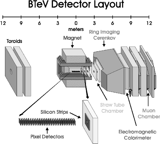
Figure 3: Layout of the BTeV Detector

The BTeV detector is shown schematically in Fig.ย 3. The covered angular region is from approximately 10 mr to 300 mr with respect to the anti-proton beam. When a B๐ตB decay of interest is contained within the acceptance of the detector, there is a high probability that the decay products of the co-produced Bยฏยฏ๐ต\bar{B} will also be within the acceptance of the detector. Furthermore, since the charged B๐ตB decay products are not degraded by multiple scattering in the detector material, which allows accurate determinations of B๐ตB decay vertices.

The key design features of BTeV include:

  • โ€ข

    A dipole centered at the interaction region placing a magnetic field on the vertex detector, allowing the use of momentum determination in the trigger. There are two open ends of the magnet. One open end allows particles to flow into the instrumented โ€œarm.โ€ The field is used by the tracking system to provide precise momentum determinations of all of the charged particles.

  • โ€ข

    A precision vertex detector based on planar pixel arrays. The outputs are used in the trigger processor to find detached heavy quark decay vertices in the first level trigger. They also provide precise and unambiguous three-dimensional space points to help reconstruct charged particles;

  • โ€ข

    Precision tracking using a combination of straw tubes and silicon microstrip detectors, inside the straws close to the beam line, where the charged particle occupancies are the largest. This system, when coupled with the pixels, provides excellent momentum and mass resolution out to 300 mr;

  • โ€ข

    Excellent charged particle identification using a Ring Imaging Cherenkov Detector (RICH). The RICH provides hadron identification from 3-70 GeV and lepton identification from 3-20 GeV, out to the full aperture of 300 mr, which is crucial since the muon detector and calorimeter do not cover the full solid angle covered by the RICH. The RICH has two independent systems sharing the same space. One has a gas (C4F8O) radiator and a Multianode Photomultiplier photon detector and the other has a liquid C5F12 radiator and a Phototube photon detector. Both systems work in the region of visible light;

  • โ€ข

    A high quality PbWO4 electromagnetic calorimeter with excellent energy resolution, position resolution and segmentation, covering up to 200 mr, capable of reconstructing final states with single photons, ฯ€osuperscript๐œ‹๐‘œ\pi^{o}โ€™s, ฮท๐œ‚\etaโ€™s or ฮทโ€ฒsuperscript๐œ‚โ€ฒ\eta^{\prime}โ€™s, and identifying electrons;

  • โ€ข

    Excellent identification of muons out to 200 mr using a dedicated detector consisting of a steel toroid instrumented with proportional tubes. This system has the ability to both identify single muons above momenta of about 10 GeV/c and supply a dimuon trigger;

  • โ€ข

    A detached vertex trigger at Level 1 using the pixel detector information, which makes BTeV efficient for most final states, including purely hadronic modes. The trigger ignores low momentum tracks that have large multiple scattering and would thereby avoid creating false secondary vertices; and

  • โ€ข

    A very high speed and high throughput data acquisition system which eliminates the need to tune the experiment to specific final states.

4 Reconstruction Efficiencies for B0โ†’(ฯโ€‹ฯ€)0โ†’superscript๐ต0superscript๐œŒ๐œ‹0B^{0}\rightarrow(\rho\pi)^{0} decays in BTeV

As stressed earlier, measuring the time dependent CP violating effects in the decays B0โ†’(ฯโ€‹ฯ€)0โ†’ฯ€+โ€‹ฯ€โˆ’โ€‹ฯ€0โ†’superscript๐ต0superscript๐œŒ๐œ‹0โ†’superscript๐œ‹superscript๐œ‹superscript๐œ‹0B^{0}\rightarrow(\rho\pi)^{0}\rightarrow\pi^{+}\pi^{-}\pi^{0} provides a theoretically clean way to determine the angle ฮฑ๐›ผ\alpha of the Unitary Triangle, as shown by Snyder and Quinn [5]. We report on the expected performance of the BTeV detector for these decays, taking into account excellent reconstruction efficiency of the ฯ€0superscript๐œ‹0\pi^{0}โ€™s that is made possible with the electromagnetic calorimeter based on PWO crystals.

Excellent mass resolution in the ฯ€0superscript๐œ‹0\pi^{0} reconstruction reduces the background significantly, particularly near the edges of the Dalitz plot where the ฯโ€‹ฯ€๐œŒ๐œ‹\rho\pi events lay. In addition, good resolution in the proper decay time is crucial to determine the angle ฮฑ๐›ผ\alpha.

The reconstruction efficiencies for Bโ†’ฯโ€‹ฯ€โ†’๐ต๐œŒ๐œ‹B\rightarrow\rho\pi were studied using GEANT3-based simulationย [22]. We generated two samples: 250,000 ฯยฑโ€‹ฯ€โˆ“superscript๐œŒplus-or-minussuperscript๐œ‹minus-or-plus\rho^{\pm}\pi^{\mp} and 250,000 ฯ0โ€‹ฯ€0superscript๐œŒ0superscript๐œ‹0\rho^{0}\pi^{0}. Both samples were generated with a mean of two Poisson distributed non-beauty interactions per beam crossing. This number of interactions per beam crossing corresponds to running at the designed Tevatron luminosity 2ร—10322superscript10322\times 10^{32}cm-2s-1 and 132ย ns bunch spacing. It should be mentioned that we used two separate Monte Carlo samples only to refine the selection procedure and determine the reconstruction efficiency and signal-to-background ratios. For the Dalitz plot analysis the interference between charged and neutral ฯ๐œŒ\rho-mesons was simulated.

The analysis relies on BTeV event reconstruction software packages, including track reconstruction based on the Kalman filter method, vertex reconstruction, and shower reconstruction.

With the use of the electromagnetic calorimeter, we would find many good ฯ€0superscript๐œ‹0\pi^{0} candidates. Photon candidates are required to have minimum reconstructed energy of 1ย GeV and pass a shower shape cut designed to reject hadronic showers. We reduce the background rate by insuring that the photon candidates are not too close to the projection of any charged tracks to the calorimeter.

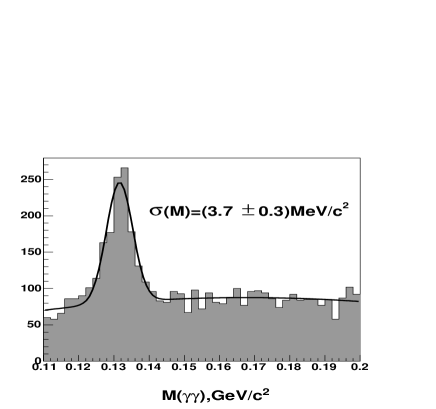
Figureย 4a shows a ฮณโ€‹ฮณ๐›พ๐›พ\gamma\gamma invariant mass distribution of the Bโ†’ฯโ€‹ฯ€โ†’๐ต๐œŒ๐œ‹B\to\rho\pi events when the pairs have energy sum greater than 5ย GeV and the vector sum of transverse momenta greater than 0.75ย GeV/c2superscript๐‘2c^{2}. The ฯ€0superscript๐œ‹0\pi^{0} signal is very clear; the ฯ€0superscript๐œ‹0\pi^{0} mass resolution in this sample is 3.7ย MeV/c2absentsuperscript๐‘2/c^{2}.

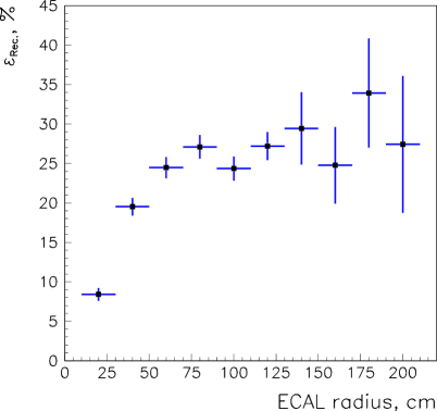
Candidate ฯ€0superscript๐œ‹0\pi^{0}โ€™s are two-photon combinations with invariant masses between 125 and 145ย MeV/c2absentsuperscript๐‘2/c^{2}. The ฯ€0superscript๐œ‹0\pi^{0} reconstruction efficiency depends on the distance from the beam line and is presented in Figureย 4b; the ฯ€0superscript๐œ‹0\pi^{0}โ€™s are taken from the B0โ†’ฯยฑโ€‹ฯ€โˆ“โ†’superscript๐ต0superscript๐œŒplus-or-minussuperscript๐œ‹minus-or-plusB^{0}\rightarrow\rho^{\pm}\pi^{\mp} events; this simulation was run with a calorimeter larger than that proposed so we could view the dependence on radius. The denominator contains all events in which the event passes the trigger, all charged tracks are reconstructed, and the combination of the two charged tracks passes some vertexing and detachment cuts. In the calculation of the efficiency we use the โ€œrightโ€ two charged tracks. However, if a pair of good charged tracks is combined with a background ฯ€0superscript๐œ‹0\pi^{0}, it does not significantly increase the efficiency.
Refer to caption
Refer to caption
Figure 4: The ฯ€0superscript๐œ‹0\pi^{0} signal in the ฮณโ€‹ฮณ๐›พ๐›พ\gamma\gamma spectrum from B0โ†’ฯ+โ€‹ฯ€โˆ’โ†’superscript๐ต0superscript๐œŒsuperscript๐œ‹B^{0}\rightarrow\rho^{+}\pi^{-} simulated events (a) and the efficiency of reconstructing the ฯ€0superscript๐œ‹0\pi^{0} as a function of distance from the beam line (b). All events considered have at least one signal B๐ตB decay. The sample includes a mean of two Poisson distributed non-beauty interactions per beam crossing.

Refer to caption

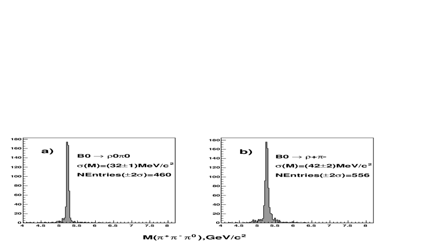
Figure 5: Invariant mass ฯ€+โ€‹ฯ€โˆ’โ€‹ฯ€0superscript๐œ‹superscript๐œ‹superscript๐œ‹0\pi^{+}\pi^{-}\pi^{0} (after cuts) for the simulated (a)ย B0โ†’ฯ0โ€‹ฯ€0โ†’superscript๐ต0superscript๐œŒ0superscript๐œ‹0B^{0}\rightarrow\rho^{0}\pi^{0} and (b)ย B0โ†’ฯ+โ€‹ฯ€โˆ’โ†’superscript๐ต0superscript๐œŒsuperscript๐œ‹B^{0}\rightarrow\rho^{+}\pi^{-} decays. Each event includes on the average two Poisson distributed non-beauty interactions per beam crossing, mixed to the beauty production interaction. The number of signal event were counted as the number of entries in the ยฑ2โ€‹ฯƒplus-or-minus2๐œŽ\pm 2\sigma interval around the B๐ตB mass, minus estimated number of background entries.

Refer to caption

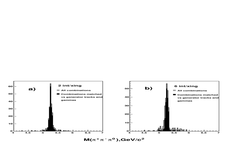
Figure 6: Invariant mass ฯ€+โ€‹ฯ€โˆ’โ€‹ฯ€0superscript๐œ‹superscript๐œ‹superscript๐œ‹0\pi^{+}\pi^{-}\pi^{0} (after cuts) matched vs generator tracks and photons, for the simulated B0โ†’ฯ+โ€‹ฯ€โˆ’โ†’superscript๐ต0superscript๐œŒsuperscript๐œ‹B^{0}\rightarrow\rho^{+}\pi^{-} at 2 and 6 interactions per crossing.

We look for events containing a secondary vertex formed by two oppositely charged tracks. One of the most important selection requirements for discriminating the signal from the background is that the events have well measured primary and secondary vertices. We demand that the primary and the secondary vertices be well defined by requiring ฯ‡2/dโ€‹oโ€‹f<2superscript๐œ’2๐‘‘๐‘œ๐‘“2\chi^{2}/dof<2 for their vertex fits. Once the primary and the B๐ตB decay vertices are determined, the distance L๐ฟL between the vertices and its error ฯƒLsubscript๐œŽ๐ฟ\sigma_{L} are computed. The quantity L/ฯƒL๐ฟsubscript๐œŽ๐ฟL/\sigma_{L} is a measure of the significance of detachement between the primary and secondary vertices. We require L/ฯƒL>4๐ฟsubscript๐œŽ๐ฟ4L/\sigma_{L}>4. The two vertices must also be separated from each other in the plane transverse to the beam. We define rtโ€‹rโ€‹aโ€‹nโ€‹sโ€‹vโ€‹eโ€‹rโ€‹sโ€‹esubscript๐‘Ÿ๐‘ก๐‘Ÿ๐‘Ž๐‘›๐‘ ๐‘ฃ๐‘’๐‘Ÿ๐‘ ๐‘’r_{transverse} in terms of the primary interaction vertex position (xP,yP,zPsubscript๐‘ฅ๐‘ƒsubscript๐‘ฆ๐‘ƒsubscript๐‘ง๐‘ƒx_{P},y_{P},z_{P}) and the secondary vertex position (xS,yS,zSsubscript๐‘ฅ๐‘†subscript๐‘ฆ๐‘†subscript๐‘ง๐‘†x_{S},y_{S},z_{S}), namely rtโ€‹rโ€‹aโ€‹nโ€‹sโ€‹vโ€‹eโ€‹rโ€‹sโ€‹e=(xPโˆ’xS)2+(yPโˆ’yS)2subscript๐‘Ÿ๐‘ก๐‘Ÿ๐‘Ž๐‘›๐‘ ๐‘ฃ๐‘’๐‘Ÿ๐‘ ๐‘’superscriptsubscript๐‘ฅ๐‘ƒsubscript๐‘ฅ๐‘†2superscriptsubscript๐‘ฆ๐‘ƒsubscript๐‘ฆ๐‘†2r_{transverse}=\sqrt{(x_{P}-x_{S})^{2}+(y_{P}-y_{S})^{2}} and reject events when rtโ€‹rโ€‹aโ€‹nโ€‹sโ€‹vโ€‹eโ€‹rโ€‹sโ€‹e<0.132subscript๐‘Ÿ๐‘ก๐‘Ÿ๐‘Ž๐‘›๐‘ ๐‘ฃ๐‘’๐‘Ÿ๐‘ ๐‘’0.132r_{t}ransverse<0.132ย mm Finaly, to insure that the charged tracks do not originate from the primary, we require that both the ฯ€+superscript๐œ‹\pi^{+} and the ฯ€โˆ’superscript๐œ‹\pi^{-} candidates have an impact parameter with respect to the primary vertex (DCA) greater than 100ย ฮผโ€‹m๐œ‡๐‘š\mu m.

When we calculate the invariant masses of the ฯ€+โ€‹ฯ€โˆ’superscript๐œ‹superscript๐œ‹\pi^{+}\pi^{-} and ฯ€ยฑโ€‹ฯ€0superscript๐œ‹plus-or-minussuperscript๐œ‹0\pi^{\pm}\pi^{0} pairs, we require at least one of them to be compatible with the ฯ๐œŒ\rho mass, that is, between 0.55 and 1.1ย GeV/c2absentsuperscript๐‘2/c^{2}. In addition, we use several kinematic cuts which reduce the background to Bโ†’ฯโ€‹ฯ€โ†’๐ต๐œŒ๐œ‹B\rightarrow\rho\pi without significantly decreasing the reconstruction efficiency. We require that ptsumsuperscriptsubscript๐‘๐‘กsump_{t}^{\rm sum} divided by the scalar sum of the ptsubscript๐‘๐‘กp_{t} values of all three particles, (ptsum/ฮฃโ€‹ptsuperscriptsubscript๐‘๐‘กsumฮฃsubscript๐‘๐‘กp_{t}^{\rm sum}/\Sigma p_{t}), be small. The vector sum ptsumsuperscriptsubscript๐‘๐‘กsump_{t}^{\rm sum} is defined with respect to the B๐ตB direction of flight which is calculated from the reconstructed primary and secondary vertices. We also make a cut on the B๐ตB proper time decay requiring it to be less than 5.5 times the B0superscript๐ต0B^{0} lifetime (tpโ€‹rโ€‹oโ€‹pโ€‹eโ€‹r/t0<5.5subscript๐‘ก๐‘๐‘Ÿ๐‘œ๐‘๐‘’๐‘Ÿsubscript๐‘ก05.5t_{proper}/t_{0}<5.5). The selection criteria are summarized in Tableย 1.

Table 1: Selection Criteria. The notation is defined in the text.
Criteria Value
Primary vertex criteria ฯ‡2<2superscript๐œ’22\chi^{2}<2
Secondary vertex criteria ฯ‡2<2superscript๐œ’22\chi^{2}<2
rtโ€‹rโ€‹aโ€‹nโ€‹sโ€‹vโ€‹eโ€‹rโ€‹sโ€‹esubscript๐‘Ÿ๐‘ก๐‘Ÿ๐‘Ž๐‘›๐‘ ๐‘ฃ๐‘’๐‘Ÿ๐‘ ๐‘’r_{transverse} (cm) 0.0132
Normalized distance L/ฯƒ๐ฟ๐œŽL/\sigma >4absent4>4
Distance L๐ฟL,ย cm <5absent5<5
DCA of track,ย ฮผ๐œ‡\mum >100absent100>100
tpโ€‹rโ€‹oโ€‹pโ€‹eโ€‹r/t0subscript๐‘ก๐‘๐‘Ÿ๐‘œ๐‘๐‘’๐‘Ÿsubscript๐‘ก0t_{proper}/t_{0} <5.5absent5.5<5.5
Eฯ€+,subscript๐ธsuperscript๐œ‹E_{\pi^{+}}, GeV >4absent4>4
Eฯ€โˆ’,subscript๐ธsuperscript๐œ‹E_{\pi^{-}}, GeV >4absent4>4
ptโ€‹(ฯ€+),subscript๐‘๐‘กsuperscript๐œ‹p_{t}(\pi^{+}),ย GeV/c๐‘c >0.4absent0.4>0.4
ptโ€‹(ฯ€โˆ’),subscript๐‘๐‘กsuperscript๐œ‹p_{t}(\pi^{-}),ย GeV/c๐‘c >0.4absent0.4>0.4
Isolation for ฮณ๐›พ\gamma,ย cm >5.4absent5.4>5.4
Eฯ€0,subscript๐ธsuperscript๐œ‹0E_{\pi^{0}}, GeV >5absent5>5
ptโ€‹(ฯ€0),subscript๐‘๐‘กsuperscript๐œ‹0p_{t}(\pi^{0}),ย GeV/c๐‘c >0.75absent0.75>0.75
ptsum/ฮฃโ€‹ptsuperscriptsubscript๐‘๐‘กsumฮฃsubscript๐‘๐‘กp_{t}^{\rm sum}/\Sigma p_{t} <0.06absent0.06<0.06
mฮณโ€‹ฮณ,subscript๐‘š๐›พ๐›พm_{\gamma\gamma}, MeV/c2superscript๐‘2c^{2} 125โˆ’145125145125-145
mฯ€โ€‹ฯ€,subscript๐‘š๐œ‹๐œ‹m_{\pi\pi}, GeV/c2superscript๐‘2c^{2} 0.55โˆ’1.10.551.10.55-1.1

The results are shown in Figureย 5 for B0โ†’ฯ0โ€‹ฯ€0โ†’superscript๐ต0superscript๐œŒ0superscript๐œ‹0B^{0}\rightarrow\rho^{0}\pi^{0} (a) and B0โ†’ฯ+โ€‹ฯ€โˆ’โ†’superscript๐ต0superscript๐œŒsuperscript๐œ‹B^{0}\rightarrow\rho^{+}\pi^{-} (b) Monte Carlo samples, respectively. The B0superscript๐ต0B^{0} mass resolution in these samples is in the range 32-42ย MeV/c2absentsuperscript๐‘2/c^{2}. The signal interval is defined as ยฑ2โ€‹ฯƒplus-or-minus2๐œŽ\pm 2\sigma around the B๐ตB mass, minus estimated background. The reconstruction efficiency is (0.18ยฑ0.02plus-or-minus0.180.020.18\pm 0.02)% for B0โ†’ฯ0โ€‹ฯ€0โ†’superscript๐ต0superscript๐œŒ0superscript๐œ‹0B^{0}\rightarrow\rho^{0}\pi^{0} and (0.22ยฑ0.02plus-or-minus0.220.020.22\pm 0.02)% for B0โ†’ฯยฑโ€‹ฯ€โˆ“โ†’superscript๐ต0superscript๐œŒplus-or-minussuperscript๐œ‹minus-or-plusB^{0}\rightarrow\rho^{\pm}\pi^{\mp}.

Similar simulation studies were repeated with six non-beauty interations per crossing mixed to the beauty production interaction to estimate reconstruction efficiency for the B0โ†’ฯ+โ€‹ฯ€โˆ’โ†’superscript๐ต0superscript๐œŒsuperscript๐œ‹B^{0}\rightarrow\rho^{+}\pi^{-} decay. Results were compared with those at two interactions per crossing. The statistics used to compare the two cases were 100,000 events.

At six interations per beam crossing the B0superscript๐ต0B^{0} mass resolution remains practicaly unchanged, as it is found to be (44ยฑ3)plus-or-minus443(44\pm 3)ย MeV/c2superscript๐‘2c^{2}. The B0โ†’ฯ+โ€‹ฯ€โˆ’โ†’superscript๐ต0superscript๐œŒsuperscript๐œ‹B^{0}\to\rho^{+}\pi^{-} reconstruction efficiency is estimated at (0.2ยฑ0.02)plus-or-minus0.20.02(0.2\pm 0.02)%. This represents the effect of only 10% as compared to two background interactions per crossing.

However, the number of false 3โ€‹ฯ€3๐œ‹3\pi combinations that would pass the cuts appears to increase somewhat as the number of non-beauty interactions per beam crossing goes up. To prove that most of the entries in the B0superscript๐ต0B^{0} mass region are true ฯ€+โ€‹ฯ€โˆ’โ€‹ฯ€0superscript๐œ‹superscript๐œ‹superscript๐œ‹0\pi^{+}\pi^{-}\pi^{0} combinations coming from the B0superscript๐ต0B^{0} decay, we have done a check against generator level information. Results of comparison are presented in Figureย 6. It is clear that the B0superscript๐ต0B^{0} signal dominates in both distributions; false 3โ€‹ฯ€3๐œ‹3\pi combinations could, in principal, mimic the signal but most of the 3โ€‹ฯ€3๐œ‹3\pi combinations are the correct ones.

Using the previously calculated reconstruction efficiency we could expect to have โˆผ1000similar-toabsent1000\sim 1000 flavor-tagged ฯยฑโ€‹ฯ€โˆ“superscript๐œŒplus-or-minussuperscript๐œ‹minus-or-plus\rho^{\pm}\pi^{\mp} events and โˆผ150similar-toabsent150\sim 150 flavor-tagged ฯ0โ€‹ฯ€0superscript๐œŒ0superscript๐œ‹0\rho^{0}\pi^{0} events per year (2ร—1072superscript1072\times 10^{7}ย s given that BTeV was assumed to run 10 months per year). The samples would include both B0superscript๐ต0B^{0} and Bยฏ0superscriptยฏ๐ต0\overline{B}^{0} decays, with proper time measurements for both states.

In principal, one can use the untagged sample in the likelihood (see Section 7) to extractย ฮฑ๐›ผ\alpha. Actually, this sample does not carry any information on ฮฑ๐›ผ\alpha but it allows to extract other parameters related to direct CP violation and helps the fit converge. This leads to an improved resolution on ฮฑ๐›ผ\alpha when the untagged sample is utilized. However, in this paper we present results obtained only with the tagged sample.

5 Signal-to-Background Ratio in B0โ†’(ฯโ€‹ฯ€)0โ†’superscript๐ต0superscript๐œŒ๐œ‹0B^{0}\rightarrow(\rho\pi)^{0} decays in BTeV

The analysis by Snyder and Quinn [5] showed that with 2,000 background free events they could always find a solution for ฮฑ๐›ผ\alpha. BTeV could have collected such a statistics within 4x10⁷ seconds (approximately 2 years). But we expect some background whose effects need to be estimated.

For a channel with a branching ratio on the order of 10-5 and efficiencies lower than 1%, it is necessary to generate at least 107 bbฬ„ background events. For this study we generated 2ร—1072superscript1072\times 10^{7} generic bbฬ„ events (Bโ†’ฯโ€‹ฯ€โ†’๐ต๐œŒ๐œ‹B\rightarrow\rho\pi channels excluded) and processed them through the GEANT3-based full detector simulation. Each event contains a mean of two Poisson distributed non-beauty interactions. Selection criteria listed in Tableย 1 are applied. To get the background estimate, we count all of the events between 5 and 7 GeV/c2superscript๐‘2c^{2}, then we scale that number down by the ratio of the signal region divided by the background selection region.

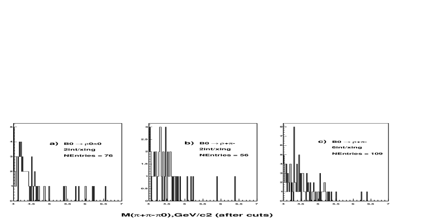
The results of the analysis are presented in Figureย 7aย andย b. The signal-to-background levels are approximetely 4:1 and 1:3 for ฯยฑโ€‹ฯ€โˆ“superscript๐œŒplus-or-minussuperscript๐œ‹minus-or-plus\rho^{\pm}\pi^{\mp} and ฯ0โ€‹ฯ€0superscript๐œŒ0superscript๐œ‹0\rho^{0}\pi^{0}, respectively, when there are on the average two interactions per crossing.

We have also investigated the effect of a larger number of interactions per crossing on the ฯ+โ€‹ฯ€โˆ’superscript๐œŒsuperscript๐œ‹\rho^{+}\pi^{-} background, similar to the study on the signal sample. We merged our background sample with an additional sample of non-beauty eventsgenerated with a Poisson distributed average of four interactions per crossing. Charged tracks in the merged events were projected onto the calorimeter, and photons from both samples were added in. Thus, the full confusion of six interactions per crossing is simulated in the calorimeter. The way we did this study, the confusion is not present in the simulation of the tracking system but separate studies show that the charged particle tracking system is reasonably robust against six interactions per crossing. The analysis then proceeded as before. We have reprocessed 1.33ร—1071.33superscript1071.33\times 10^{7} events and have compared the results corresponding to this statistics at two or six interactions per crossing. The background to B0โ†’ฯ+โ€‹ฯ€โˆ’โ†’superscript๐ต0superscript๐œŒsuperscript๐œ‹B^{0}\to\rho^{+}\pi^{-} at six interactions per crossing is presented in Figureย 7c). We have found that at six interactions per crossing the background to B0โ†’ฯ+โ€‹ฯ€โˆ’โ†’superscript๐ต0superscript๐œŒsuperscript๐œ‹B^{0}\to\rho^{+}\pi^{-} increased to 109 events, at compared to 56 events at two interactions per crossing. This demonstrates that the background could increase at six interactions per crossing but the effect is expected to be about aย factorย ofย 2.

Refer to caption

Figure 7: Background ฯ€+โ€‹ฯ€โˆ’โ€‹ฯ€0superscript๐œ‹superscript๐œ‹superscript๐œ‹0\pi^{+}\pi^{-}\pi^{0} invariant mass for B0โ†’ฯ0โ€‹ฯ€0โ†’superscript๐ต0superscript๐œŒ0superscript๐œ‹0B^{0}\rightarrow\rho^{0}\pi^{0} and B0โ†’ฯ+โ€‹ฯ€โˆ’โ†’superscript๐ต0superscript๐œŒsuperscript๐œ‹B^{0}\rightarrow\rho^{+}\pi^{-} at 2 interactions per crossing (a,b), and B0โ†’ฯ+โ€‹ฯ€โˆ’โ†’superscript๐ต0superscript๐œŒsuperscript๐œ‹B^{0}\rightarrow\rho^{+}\pi^{-} at 6 interactions per crossing (c)

6 Representation of amplitudes and phenomenological inputs

6.1 Classification of the amplitudes

In this section we first define the formalism. Next, we estimate parameter values so that the simulation is as close as possible to reality.

Amplitudes of neutral B0superscript๐ต0B^{0} meson decay to ฯโ€‹ฯ€๐œŒ๐œ‹\rho\pi are represented in the form

|B0โŸฉ=fiaiโ€‹j,{ij}={+โˆ’},{โˆ’+},{00},|B^{0}\rangle=f_{i}a_{ij},\qquad\{ij\}=\{+-\},\{-+\},\{00\}, (7)
aiโ€‹j=(โˆ’eโˆ’iโ€‹ฮฑโ€‹Tiโ€‹j+Piโ€‹j)โ€‹eโˆ’iโ€‹ฮฒ,subscript๐‘Ž๐‘–๐‘—superscript๐‘’i๐›ผsubscript๐‘‡๐‘–๐‘—subscript๐‘ƒ๐‘–๐‘—superscript๐‘’i๐›ฝa_{ij}=\left(-e^{-{\rm i}\alpha}T_{ij}+P_{ij}\right)e^{-{\rm i}\beta}, (8)

where Tiโ€‹jsubscript๐‘‡๐‘–๐‘—T_{ij} and Piโ€‹jsubscript๐‘ƒ๐‘–๐‘—P_{ij} give tree and penguin amplitudes, correspondingly, as depicted in Fig. 8 extracted from [23].

Refer to caption
Refer to caption
Figure 8: The tree (left) and penguin (right) diagrams for the B0โ†’ฯ+โ€‹ฯ€โˆ’โ†’superscript๐ต0superscript๐œŒsuperscript๐œ‹B^{0}\to\rho^{+}\pi^{-} (B0โ†’ฯโˆ’โ€‹ฯ€+โ†’superscript๐ต0superscript๐œŒsuperscript๐œ‹B^{0}\to\rho^{-}\pi^{+}) decays.

The fksubscript๐‘“๐‘˜f_{k} represents the relativistic Breit-Wigner form for ฯโ†’ฯ€โ€‹ฯ€โ†’๐œŒ๐œ‹๐œ‹\rho\to\pi\pi

fk=cโ€‹oโ€‹sโ€‹(ฮธk)sโˆ’mฯ2+iโ€‹ฮ โ€‹(s),subscript๐‘“๐‘˜๐‘๐‘œ๐‘ subscript๐œƒ๐‘˜๐‘ subscriptsuperscript๐‘š2๐œŒ๐‘–ฮ ๐‘ f_{k}=\frac{cos(\theta_{k})}{s-m^{2}_{\rho}+i\Pi(s)}, (9)

where s๐‘ s is the square of the invariant mass (ฯ€1,ฯ€2subscript๐œ‹1subscript๐œ‹2\pi_{1},\pi_{2}) and ฮธksubscript๐œƒ๐‘˜\theta_{k} is the angle between a decay pion and the line of flight of the ฯ๐œŒ\rho. The function ฮ โ€‹(s)ฮ ๐‘ \Pi(s) is defined as

ฮ โ€‹(s)=mฯ2sโ€‹(pโ€‹(s)pโ€‹(mฯ2))3โ€‹ฮ“โ€‹(mฯ2),pโ€‹(s)=s/4โˆ’mฯ2,formulae-sequenceฮ ๐‘ subscriptsuperscript๐‘š2๐œŒ๐‘ superscript๐‘๐‘ ๐‘subscriptsuperscript๐‘š2๐œŒ3ฮ“subscriptsuperscript๐‘š2๐œŒ๐‘๐‘ ๐‘ 4subscriptsuperscript๐‘š2๐œŒ\Pi(s)=\frac{m^{2}_{\rho}}{\sqrt{s}}\left(\frac{p(s)}{p(m^{2}_{\rho})}\right)^{3}\Gamma(m^{2}_{\rho}),\qquad p(s)=\sqrt{s/4-m^{2}_{\rho}}, (10)

where mฯsubscript๐‘š๐œŒm_{\rho} is the ฯ๐œŒ\rho mass and ฮ“ฮ“\Gamma is the width.

The amplitudes aiโ€‹jsubscript๐‘Ž๐‘–๐‘—a_{ij} for B0superscript๐ต0B^{0} and Bยฏ0superscriptยฏ๐ต0\overline{B}^{0} decay are written as a sum of tree (T๐‘‡T) and penguin (P๐‘ƒP) contributions as

a+โˆ’=โˆ’eiโ€‹ฮณโ€‹T+โˆ’+eโˆ’iโ€‹ฮฒโ€‹P+โˆ’subscript๐‘Žabsentsuperscript๐‘’๐‘–๐›พsuperscript๐‘‡absentsuperscript๐‘’๐‘–๐›ฝsuperscript๐‘ƒabsent\displaystyle a_{+-}=-e^{i\gamma}T^{+-}+e^{-i\beta}P^{+-}
aโˆ’+=โˆ’eiโ€‹ฮณโ€‹Tโˆ’++eโˆ’iโ€‹ฮฒโ€‹Pโˆ’+subscript๐‘Žabsentsuperscript๐‘’๐‘–๐›พsuperscript๐‘‡absentsuperscript๐‘’๐‘–๐›ฝsuperscript๐‘ƒabsent\displaystyle a_{-+}=-e^{i\gamma}T^{-+}+e^{-i\beta}P^{-+}
a00=โˆ’eiโ€‹ฮณโ€‹T00+eโˆ’iโ€‹ฮฒโ€‹P00subscript๐‘Ž00superscript๐‘’๐‘–๐›พsuperscript๐‘‡00superscript๐‘’๐‘–๐›ฝsuperscript๐‘ƒ00\displaystyle a_{00}=-e^{i\gamma}T^{00}+e^{-i\beta}P^{00}
aยฏ+โˆ’=โˆ’eโˆ’iโ€‹ฮณโ€‹Tโˆ’++eiโ€‹ฮฒโ€‹Pโˆ’+subscriptยฏ๐‘Žabsentsuperscript๐‘’๐‘–๐›พsuperscript๐‘‡absentsuperscript๐‘’๐‘–๐›ฝsuperscript๐‘ƒabsent\displaystyle\bar{a}_{+-}=-e^{-i\gamma}T^{-+}+e^{i\beta}P^{-+}
aยฏโˆ’+=โˆ’eโˆ’iโ€‹ฮณโ€‹T+โˆ’+eiโ€‹ฮฒโ€‹P+โˆ’subscriptยฏ๐‘Žabsentsuperscript๐‘’๐‘–๐›พsuperscript๐‘‡absentsuperscript๐‘’๐‘–๐›ฝsuperscript๐‘ƒabsent\displaystyle\bar{a}_{-+}=-e^{-i\gamma}T^{+-}+e^{i\beta}P^{+-}
aยฏ00=โˆ’eโˆ’iโ€‹ฮณโ€‹T00+eiโ€‹ฮฒโ€‹P00,subscriptยฏ๐‘Ž00superscript๐‘’๐‘–๐›พsuperscript๐‘‡00superscript๐‘’๐‘–๐›ฝsuperscript๐‘ƒ00\displaystyle\bar{a}_{00}=-e^{-i\gamma}T^{00}+e^{i\beta}P^{00}, (11)

where ฮณ๐›พ\gamma and ฮฒ๐›ฝ\beta are the usual CKM angles and ฮฑ+ฮฒ+ฮณ=ฯ€๐›ผ๐›ฝ๐›พ๐œ‹\alpha+\beta+\gamma=\pi. Using both isospin symmetry and the fact that the Penguin amplitude is a pure ฮ”โ€‹I=1/2ฮ”๐ผ12\Delta I=1/2 transition leads to the replacement

P00=โˆ’12โ€‹(P+โˆ’+Pโˆ’+).subscript๐‘ƒ0012subscript๐‘ƒabsentsubscript๐‘ƒabsentP_{00}=-\frac{1}{2}\left(P_{+-}+P_{-+}\right). (12)

For the tree diagrams after Fierz transformation one naively gets

T00=12โ€‹a2a1โ€‹(T+โˆ’+Tโˆ’+),subscript๐‘‡0012subscript๐‘Ž2subscript๐‘Ž1subscript๐‘‡absentsubscript๐‘‡absentT_{00}=\frac{1}{2}\,\frac{a_{2}}{a_{1}}\left(T_{+-}+T_{-+}\right), (13)

where factors a1,2subscript๐‘Ž12a_{1,2} represent contributions due to gluon corrections to the weak interactions of quarks and depend on renormalization scale. The corresponding Lagrangian is approximated by

โ„’=GF2โ€‹2โ€‹Vuโ€‹dโ€‹Vuโ€‹bโˆ—โ€‹Cยฑโ€‹(bยฏiโ€‹๐’ชฮผโ€‹uj)โ€‹(uยฏkโ€‹๐’ชฮผโ€‹dl)โ€‹[ฮดjiโ€‹ฮดlkยฑฮดliโ€‹ฮดjk],โ„’subscript๐บF22subscript๐‘‰๐‘ข๐‘‘subscriptsuperscript๐‘‰๐‘ข๐‘subscript๐ถplus-or-minussubscriptยฏ๐‘๐‘–subscript๐’ช๐œ‡superscript๐‘ข๐‘—subscriptยฏ๐‘ข๐‘˜superscript๐’ช๐œ‡superscript๐‘‘๐‘™delimited-[]plus-or-minussubscriptsuperscript๐›ฟ๐‘–๐‘—subscriptsuperscript๐›ฟ๐‘˜๐‘™subscriptsuperscript๐›ฟ๐‘–๐‘™subscriptsuperscript๐›ฟ๐‘˜๐‘—{\mathcal{L}}=\frac{G_{\rm F}}{2\sqrt{2}}\,V_{ud}V^{*}_{ub}\,C_{\pm}\,(\bar{b}_{i}{\mathcal{O}}_{\mu}u^{j})\,(\bar{u}_{k}{\mathcal{O}}^{\mu}d^{l})\,\left[\delta^{i}_{j}\delta^{k}_{l}\pm\delta^{i}_{l}\delta^{k}_{j}\right], (14)

where indices mark SU(3)-colors, and the factors are defined as

a1=12โ€‹Ncโ€‹[C+โ€‹(Nc+1)+Cโˆ’โ€‹(Ncโˆ’1)],a2=12โ€‹Ncโ€‹[C+โ€‹(Nc+1)โˆ’Cโˆ’โ€‹(Ncโˆ’1)]formulae-sequencesubscript๐‘Ž112subscript๐‘๐‘delimited-[]subscript๐ถsubscript๐‘๐‘1subscript๐ถsubscript๐‘๐‘1subscript๐‘Ž212subscript๐‘๐‘delimited-[]subscript๐ถsubscript๐‘๐‘1subscript๐ถsubscript๐‘๐‘1a_{1}=\frac{1}{2N_{c}}\,[C_{+}(N_{c}+1)+C_{-}(N_{c}-1)],\qquad a_{2}=\frac{1}{2N_{c}}\,[C_{+}(N_{c}+1)-C_{-}(N_{c}-1)] (15)

where Nc=3subscript๐‘๐‘3N_{c}=3. In the limit of neglecting the gluon corrections we get

Cยฑ=1,a1=1,a2=1Nc.formulae-sequencesubscript๐ถplus-or-minus1formulae-sequencesubscript๐‘Ž11subscript๐‘Ž21subscript๐‘๐‘C_{\pm}=1,\qquad a_{1}=1,\qquad a_{2}=\frac{1}{N_{c}}.

However, the corrections taking into account the renormalization group dependence on a decay scale put the ratio a2/a1subscript๐‘Ž2subscript๐‘Ž1a_{2}/a_{1} to a negative value approximately given by

a2a1=โˆ’0.25ยฑ0.05.subscript๐‘Ž2subscript๐‘Ž1plus-or-minus0.250.05\frac{a_{2}}{a_{1}}=-0.25\pm 0.05. (16)

In fact, as was shown in [24] and [25], expressions (15) following from the factorization hypothesis can be significantly modified by โ€œnon-factorizable effectsโ€ in the complex phase. This means that only the absolute value of the ratio

|a2a1|=0.25ยฑ0.05subscript๐‘Ž2subscript๐‘Ž1plus-or-minus0.250.05\left|\frac{a_{2}}{a_{1}}\right|=0.25\pm 0.05

is reliable. The value of the phase is not realiably predicted by the theory but is roughly estimated to be about 45โˆ˜superscript4545^{\circ}.

Corrections in (12) and (13) due to isospin symmetry breaking are considered to be negligible [23] and they are not included in the following simulations.

6.2 Phenomenological constraints on the parameters

A phenomenological analysis of possible values for the amplitudes in (7) has been performed in [23] and [26]. It is based on a global fit to the measured rates assuming SU(3)-flavor symmetry for Bโ†’ฯโ€‹ฯ€โ†’๐ต๐œŒ๐œ‹B\to\rho\pi, Bโ†’Kโˆ—โ€‹ฯ€โ†’๐ตsuperscript๐พ๐œ‹B\to K^{*}\pi and Bโ†’ฯโ€‹Kโ†’๐ต๐œŒ๐พB\to\rho K decays. The analysis gives approximately twice enhancement of penguin amplitudes in comparison with QCD expectations [25]. The preferable values of amplitudes with theoretical expectations of uncertainties are summarized in Tableย 2, which has two sets of parameters we use in our modelling of the signal.

Table 2: Amplitudes in units of T+โˆ’subscript๐‘‡absentT_{+-} set to 111 and expected uncertainties from fits in [23] and [26].
ย ย ย ย ย Parameter ย ย ย ย ย Set I ย ย ย ย ย Set II Theor. uncertainties or limits
|Tโˆ’+|subscript๐‘‡absent\quad|T_{-+}| 0.8 0.8 0.63โˆ’0.90.630.90.63-0.9
argโก[Tโˆ’+]subscript๐‘‡absent\arg\left[T_{-+}\right] โˆ’20โˆ˜superscript20-20^{\circ} โˆ’20โˆ˜superscript20-20^{\circ} ยฑ10โˆ˜plus-or-minussuperscript10\pm 10^{\circ}
|P+โˆ’|subscript๐‘ƒabsent\quad|P_{+-}| 0.18 0.18 ยฑ0.05plus-or-minus0.05\pm 0.05
argโก[P+โˆ’]subscript๐‘ƒabsent\arg[P_{+-}] 30โˆ˜superscript3030^{\circ} 30โˆ˜superscript3030^{\circ} ยฑ30โˆ˜plus-or-minussuperscript30\pm 30^{\circ}
|Pโˆ’+Tโˆ’+|subscript๐‘ƒabsentsubscript๐‘‡absent\quad\displaystyle\left|\frac{P_{-+}}{T_{-+}}\right| 0.28 0.28 0.14โˆ’0.320.140.320.14-0.32
argโก[Pโˆ’+Tโˆ’+]subscript๐‘ƒabsentsubscript๐‘‡absent\displaystyle\arg\left[\frac{P_{-+}}{T_{-+}}\right] 80โˆ˜superscript8080^{\circ} 130โˆ˜superscript130130^{\circ} ยฑ60โˆ˜plus-or-minussuperscript60\pm 60^{\circ}
|a2a1|subscript๐‘Ž2subscript๐‘Ž1\quad\displaystyle\left|\frac{a_{2}}{a_{1}}\right| 0.25 0.25 0.18โˆ’0.320.180.320.18-0.32
argโก[a2a1]subscript๐‘Ž2subscript๐‘Ž1\displaystyle\arg\left[\frac{a_{2}}{a_{1}}\right] 45โˆ˜ 45โˆ˜ 0โˆ’2โ€‹ฯ€02๐œ‹0-2\pi
ฮฑ๐›ผ\alpha 88โˆ˜superscript8888^{\circ} 100โˆ˜superscript100100^{\circ} 80โˆ˜โˆ’110โˆ˜superscript80superscript11080^{\circ}-110^{\circ}

The value of |Tโˆ’+|subscript๐‘‡absent|T_{-+}| is ordinary fixed by the factorization hypothesis [23], so that it is equal to the ratio of decay constants fฯ€/fฯโ‰ˆ0.63subscript๐‘“๐œ‹subscript๐‘“๐œŒ0.63f_{\pi}/f_{\rho}\approx 0.63, while the ratio fitted by SU(3) ansatz results in a greater value of about 0.70.70.7. Nevertheless, we fix this parameter to 0.80.80.8, reproducing the mean magnitude of branching fractions. The uncertainties of complex phases are not given explicitly in [23] and [26], but we expect them to be lower than 30โˆ˜superscript3030^{\circ} at fixed absolute values of penguin-to-tree ratios. The amplitude of B0โ†’ฯ0โ€‹ฯ€0โ†’superscript๐ต0superscript๐œŒ0superscript๐œ‹0B^{0}\to\rho^{0}\pi^{0} is constructed in accordance with (12), (13) and (16).

Now we make the transition to the estimate of parameter values in the simulation and to the comparison with the existing experimental results.

The overall normalization is tuned to the experimental sum of CP-averaged branching ratios

โ„ฌฯโ€‹ฯ€ยฑโˆ“=โ„ฌฯโ€‹ฯ€+โˆ’+โ„ฌฯโ€‹ฯ€โˆ’+=(24.0ยฑ2.5)ร—10โˆ’6,subscriptsuperscriptโ„ฌplus-or-minusabsentminus-or-plus๐œŒ๐œ‹subscriptsuperscriptโ„ฌabsent๐œŒ๐œ‹subscriptsuperscriptโ„ฌabsent๐œŒ๐œ‹plus-or-minus24.02.5superscript106{\mathcal{B}}^{\pm\mp}_{\rho\pi}={\mathcal{B}}^{+-}_{\rho\pi}+{\mathcal{B}}^{-+}_{\rho\pi}=(24.0\pm 2.5)\times 10^{-6},

where

โ„ฌฯโ€‹ฯ€+โˆ’=12โ€‹{โ„ฌโ€‹[B0โ†’ฯ+โ€‹ฯ€โˆ’]+โ„ฌโ€‹[Bยฏ0โ†’ฯโˆ’โ€‹ฯ€+]}=(13.9ยฑ2.2)ร—10โˆ’6,subscriptsuperscriptโ„ฌabsent๐œŒ๐œ‹12โ„ฌdelimited-[]โ†’superscript๐ต0superscript๐œŒsuperscript๐œ‹โ„ฌdelimited-[]โ†’superscriptยฏ๐ต0superscript๐œŒsuperscript๐œ‹plus-or-minus13.92.2superscript106{\mathcal{B}}^{+-}_{\rho\pi}=\frac{1}{2}\left\{{\mathcal{B}}[B^{0}\to\rho^{+}\pi^{-}]+{\mathcal{B}}[\bar{B}^{0}\to\rho^{-}\pi^{+}]\right\}=(13.9\pm 2.2)\times 10^{-6},
โ„ฌฯโ€‹ฯ€โˆ’+=12โ€‹{โ„ฌโ€‹[B0โ†’ฯโˆ’โ€‹ฯ€+]+โ„ฌโ€‹[Bยฏ0โ†’ฯ+โ€‹ฯ€โˆ’]}=(10.1ยฑ2.1)ร—10โˆ’6.subscriptsuperscriptโ„ฌabsent๐œŒ๐œ‹12โ„ฌdelimited-[]โ†’superscript๐ต0superscript๐œŒsuperscript๐œ‹โ„ฌdelimited-[]โ†’superscriptยฏ๐ต0superscript๐œŒsuperscript๐œ‹plus-or-minus10.12.1superscript106{\mathcal{B}}^{-+}_{\rho\pi}=\frac{1}{2}\left\{{\mathcal{B}}[B^{0}\to\rho^{-}\pi^{+}]+{\mathcal{B}}[\bar{B}^{0}\to\rho^{+}\pi^{-}]\right\}=(10.1\pm 2.1)\times 10^{-6}.

For example, taking the set I of parameters we get

โ„ฌโ€‹[B0โ†’ฯ+โ€‹ฯ€โˆ’]=16.5ร—10โˆ’6,โ„ฌโ€‹[B0โ†’ฯโˆ’โ€‹ฯ€+]=14.1ร—10โˆ’6,โ„ฌโ€‹[B0โ†’ฯ0โ€‹ฯ€0]=0.9ร—10โˆ’6,formulae-sequenceโ„ฌdelimited-[]โ†’superscript๐ต0superscript๐œŒsuperscript๐œ‹16.5superscript106formulae-sequenceโ„ฌdelimited-[]โ†’superscript๐ต0superscript๐œŒsuperscript๐œ‹14.1superscript106โ„ฌdelimited-[]โ†’superscript๐ต0superscript๐œŒ0superscript๐œ‹00.9superscript106{\mathcal{B}}[B^{0}\to\rho^{+}\pi^{-}]=16.5\times 10^{-6},\qquad{\mathcal{B}}[B^{0}\to\rho^{-}\pi^{+}]=14.1\times 10^{-6},\qquad{\mathcal{B}}[B^{0}\to\rho^{0}\pi^{0}]=0.9\times 10^{-6},

and

โ„ฌโ€‹[Bยฏ0โ†’ฯ+โ€‹ฯ€โˆ’]=4.6ร—10โˆ’6,โ„ฌโ€‹[Bยฏ0โ†’ฯโˆ’โ€‹ฯ€+]=11.6ร—10โˆ’6,โ„ฌโ€‹[Bยฏ0โ†’ฯ0โ€‹ฯ€0]=1.4ร—10โˆ’6,formulae-sequenceโ„ฌdelimited-[]โ†’superscriptยฏ๐ต0superscript๐œŒsuperscript๐œ‹4.6superscript106formulae-sequenceโ„ฌdelimited-[]โ†’superscriptยฏ๐ต0superscript๐œŒsuperscript๐œ‹11.6superscript106โ„ฌdelimited-[]โ†’superscriptยฏ๐ต0superscript๐œŒ0superscript๐œ‹01.4superscript106{\mathcal{B}}[\bar{B}^{0}\to\rho^{+}\pi^{-}]=4.6\times 10^{-6},\qquad{\mathcal{B}}[\bar{B}^{0}\to\rho^{-}\pi^{+}]=11.6\times 10^{-6},\qquad{\mathcal{B}}[\bar{B}^{0}\to\rho^{0}\pi^{0}]=1.4\times 10^{-6},

which should be compared with experimental averages from BELLE, BABAR and CLEO in [23] and [26]

โ„ฌโ€‹[B0โ†’ฯ+โ€‹ฯ€โˆ’]=(16.5โˆ’2.8+3.1)ร—10โˆ’6,โ„ฌโ€‹[B0โ†’ฯโˆ’โ€‹ฯ€+]=(15.4โˆ’2.9+3.2)ร—10โˆ’6,formulae-sequenceโ„ฌdelimited-[]โ†’superscript๐ต0superscript๐œŒsuperscript๐œ‹subscriptsuperscript16.53.12.8superscript106โ„ฌdelimited-[]โ†’superscript๐ต0superscript๐œŒsuperscript๐œ‹subscriptsuperscript15.43.22.9superscript106{\mathcal{B}}[B^{0}\to\rho^{+}\pi^{-}]=(16.5^{+3.1}_{-2.8})\times 10^{-6},\qquad{\mathcal{B}}[B^{0}\to\rho^{-}\pi^{+}]=(15.4^{+3.2}_{-2.9})\times 10^{-6},\qquad

and

โ„ฌโ€‹[B0โ†’ฯ+โ€‹ฯ€โˆ’]=(4.8โˆ’2.3+2.6)ร—10โˆ’6,โ„ฌโ€‹[B0โ†’ฯโˆ’โ€‹ฯ€+]=(11.4โˆ’2.6+2.8)ร—10โˆ’6.formulae-sequenceโ„ฌdelimited-[]โ†’superscript๐ต0superscript๐œŒsuperscript๐œ‹subscriptsuperscript4.82.62.3superscript106โ„ฌdelimited-[]โ†’superscript๐ต0superscript๐œŒsuperscript๐œ‹subscriptsuperscript11.42.82.6superscript106{\mathcal{B}}[B^{0}\to\rho^{+}\pi^{-}]=(4.8^{+2.6}_{-2.3})\times 10^{-6},\qquad{\mathcal{B}}[B^{0}\to\rho^{-}\pi^{+}]=(11.4^{+2.8}_{-2.6})\times 10^{-6}.\qquad

The above branching ratios give CP-averaged values of

โ„ฌฯโ€‹ฯ€+โˆ’=14.0ร—10โˆ’6,โ„ฌฯโ€‹ฯ€โˆ’+=9.3ร—10โˆ’6formulae-sequencesubscriptsuperscriptโ„ฌabsent๐œŒ๐œ‹14.0superscript106subscriptsuperscriptโ„ฌabsent๐œŒ๐œ‹9.3superscript106{\mathcal{B}}^{+-}_{\rho\pi}=14.0\times 10^{-6},\qquad{\mathcal{B}}^{-+}_{\rho\pi}=9.3\times 10^{-6}

for the charged modes, while for the neutral mode we have

โ„ฌฯโ€‹ฯ€00=12โ€‹{โ„ฌโ€‹[B0โ†’ฯ0โ€‹ฯ€0]+โ„ฌโ€‹[Bยฏ0โ†’ฯ0โ€‹ฯ€0]}=1.2ร—10โˆ’6subscriptsuperscriptโ„ฌ00๐œŒ๐œ‹12โ„ฌdelimited-[]โ†’superscript๐ต0superscript๐œŒ0superscript๐œ‹0โ„ฌdelimited-[]โ†’superscriptยฏ๐ต0superscript๐œŒ0superscript๐œ‹01.2superscript106{\mathcal{B}}^{00}_{\rho\pi}=\frac{1}{2}\left\{{\mathcal{B}}[B^{0}\to\rho^{0}\pi^{0}]+{\mathcal{B}}[\bar{B}^{0}\to\rho^{0}\pi^{0}]\right\}=1.2\times 10^{-6}

are consistent with the experimental value

โ„ฌฯโ€‹ฯ€00=(1.7ยฑ0.8)ร—10โˆ’6<2.5ร—10โˆ’6โ€‹at 95% C.L.subscriptsuperscriptโ„ฌ00๐œŒ๐œ‹plus-or-minus1.70.8superscript1062.5superscript106at 95% C.L.{\mathcal{B}}^{00}_{\rho\pi}=(1.7\pm 0.8)\times 10^{-6}<2.5\times 10^{-6}\;\mbox{at 95\% C.L.}

Note, that the neutral CP-averaged mode weakly depends on the complex phase of a2/a1subscript๐‘Ž2subscript๐‘Ž1a_{2}/a_{1}, but branching ratios of B0superscript๐ต0B^{0} and Bยฏ0superscriptยฏ๐ต0\bar{B}^{0} strongly depend on that phase: for instance, putting argโก[a2/a1]=ฯ€subscript๐‘Ž2subscript๐‘Ž1๐œ‹\arg[a_{2}/a_{1}]=\pi gives โ„ฌโ€‹[B0โ†’ฯ0โ€‹ฯ€0]=2.1ร—10โˆ’6โ„ฌdelimited-[]โ†’superscript๐ต0superscript๐œŒ0superscript๐œ‹02.1superscript106{\mathcal{B}}[B^{0}\to\rho^{0}\pi^{0}]=2.1\times 10^{-6} and โ„ฌโ€‹[Bยฏ0โ†’ฯ0โ€‹ฯ€0]=0.2ร—10โˆ’6โ„ฌdelimited-[]โ†’superscriptยฏ๐ต0superscript๐œŒ0superscript๐œ‹00.2superscript106{\mathcal{B}}[\bar{B}^{0}\to\rho^{0}\pi^{0}]=0.2\times 10^{-6}.

The time-dependent CP asymmetry is given by

aCโ€‹Pยฑsubscriptsuperscript๐‘Žplus-or-minus๐ถ๐‘ƒ\displaystyle a^{\pm}_{CP} =\displaystyle= ฮ“โ€‹(Bยฏ0โ€‹(t)โ†’ฯยฑโ€‹ฯ€โˆ“)โˆ’ฮ“โ€‹(B0โ€‹(t)โ†’ฯยฑโ€‹ฯ€โˆ“)ฮ“โ€‹(Bยฏ0โ€‹(t)โ†’ฯยฑโ€‹ฯ€โˆ“)+ฮ“โ€‹(B0โ€‹(t)โ†’ฯยฑโ€‹ฯ€โˆ“)=ฮ“โ†’superscriptยฏ๐ต0๐‘กsuperscript๐œŒplus-or-minussuperscript๐œ‹minus-or-plusฮ“โ†’superscript๐ต0๐‘กsuperscript๐œŒplus-or-minussuperscript๐œ‹minus-or-plusฮ“โ†’superscriptยฏ๐ต0๐‘กsuperscript๐œŒplus-or-minussuperscript๐œ‹minus-or-plusฮ“โ†’superscript๐ต0๐‘กsuperscript๐œŒplus-or-minussuperscript๐œ‹minus-or-plusabsent\displaystyle\frac{\Gamma(\overline{B}^{0}(t)\to\rho^{\pm}\pi^{\mp})-\Gamma(B^{0}(t)\to\rho^{\pm}\pi^{\mp})}{\Gamma(\overline{B}^{0}(t)\to\rho^{\pm}\pi^{\mp})+\Gamma(B^{0}(t)\to\rho^{\pm}\pi^{\mp})}= (17)
=(Sฯโ€‹ฯ€ยฑฮ”โ€‹Sฯโ€‹ฯ€)โ€‹sinโก(ฮ”โ€‹mdโ€‹t)โˆ’(Cฯโ€‹ฯ€ยฑฮ”โ€‹Cฯโ€‹ฯ€)โ€‹cosโก(ฮ”โ€‹mdโ€‹t).absentplus-or-minussubscript๐‘†๐œŒ๐œ‹ฮ”subscript๐‘†๐œŒ๐œ‹ฮ”subscript๐‘š๐‘‘๐‘กplus-or-minussubscript๐ถ๐œŒ๐œ‹ฮ”subscript๐ถ๐œŒ๐œ‹ฮ”subscript๐‘š๐‘‘๐‘ก\displaystyle=(S_{\rho\pi}\pm\Delta S_{\rho\pi})\sin(\Delta m_{d}t)-(C_{\rho\pi}\pm\Delta C_{\rho\pi})\cos(\Delta m_{d}t).

In this formula Sฯโ€‹ฯ€subscript๐‘†๐œŒ๐œ‹S_{\rho\pi} and Cฯโ€‹ฯ€subscript๐ถ๐œŒ๐œ‹C_{\rho\pi} represent mixing-induced CP violation and flavor-dependent direct CP violation, respectively. The value of ฮ”โ€‹Sฯโ€‹ฯ€ฮ”subscript๐‘†๐œŒ๐œ‹\Delta S_{\rho\pi} and ฮ”โ€‹Cฯโ€‹ฯ€ฮ”subscript๐ถ๐œŒ๐œ‹\Delta C_{\rho\pi} are CP-conserving. The ฮ”โ€‹Cฯโ€‹ฯ€ฮ”subscript๐ถ๐œŒ๐œ‹\Delta C_{\rho\pi} characterizes the asymmetry between rates ฮ“โ€‹(B0โ†’ฯ+โ€‹ฯ€โˆ’)+ฮ“โ€‹(Bยฏ0โ†’ฯโˆ’โ€‹ฯ€+)ฮ“โ†’superscript๐ต0superscript๐œŒsuperscript๐œ‹ฮ“โ†’superscriptยฏ๐ต0superscript๐œŒsuperscript๐œ‹\Gamma(B^{0}\to\rho^{+}\pi^{-})+\Gamma(\overline{B}^{0}\to\rho^{-}\pi^{+}) and ฮ“โ€‹(B0โ†’ฯโˆ’โ€‹ฯ€+)+ฮ“โ€‹(Bยฏ0โ†’ฯ+โ€‹ฯ€โˆ’)ฮ“โ†’superscript๐ต0superscript๐œŒsuperscript๐œ‹ฮ“โ†’superscriptยฏ๐ต0superscript๐œŒsuperscript๐œ‹\Gamma(B^{0}\to\rho^{-}\pi^{+})+\Gamma(\overline{B}^{0}\to\rho^{+}\pi^{-}) at t=0๐‘ก0t=0, i.e. at initial moment of evolution, while ฮ”โ€‹Sฯโ€‹ฯ€ฮ”subscript๐‘†๐œŒ๐œ‹\Delta S_{\rho\pi} indicates mixing of decays at tโ‰ 0๐‘ก0t\neq 0, and as we have found, it strongly depends on both the relative strong phase of penguin with respect to tree amplitude in ฯโˆ’โ€‹ฯ€+superscript๐œŒsuperscript๐œ‹\rho^{-}\pi^{+} mode (the parameter argโ€‹[Pโˆ’+/Tโˆ’+]argdelimited-[]subscript๐‘ƒabsentsubscript๐‘‡absent\mbox{arg}[P_{-+}/T_{-+}]) and the CKM angle ฮฑ๐›ผ\alpha.

Time-integrated asymmetries are given by

Aฯโ€‹ฯ€+โˆ’=โˆ’Aฯโ€‹ฯ€+Cฯโ€‹ฯ€+Aฯโ€‹ฯ€โ€‹ฮ”โ€‹Cฯโ€‹ฯ€1+ฮ”โ€‹Cฯโ€‹ฯ€+Aฯโ€‹ฯ€โ€‹Cฯโ€‹ฯ€=Nโ€‹(Bยฏ0โ†’ฯโˆ’โ€‹ฯ€+)โˆ’Nโ€‹(B0โ†’ฯ+โ€‹ฯ€โˆ’)Nโ€‹(Bยฏ0โ†’ฯโˆ’โ€‹ฯ€+)+Nโ€‹(B0โ†’ฯ+โ€‹ฯ€โˆ’),subscriptsuperscript๐ดabsent๐œŒ๐œ‹subscript๐ด๐œŒ๐œ‹subscript๐ถ๐œŒ๐œ‹subscript๐ด๐œŒ๐œ‹ฮ”subscript๐ถ๐œŒ๐œ‹1ฮ”subscript๐ถ๐œŒ๐œ‹subscript๐ด๐œŒ๐œ‹subscript๐ถ๐œŒ๐œ‹๐‘โ†’superscriptยฏ๐ต0superscript๐œŒsuperscript๐œ‹๐‘โ†’superscript๐ต0superscript๐œŒsuperscript๐œ‹๐‘โ†’superscriptยฏ๐ต0superscript๐œŒsuperscript๐œ‹๐‘โ†’superscript๐ต0superscript๐œŒsuperscript๐œ‹A^{+-}_{\rho\pi}=-\frac{A_{\rho\pi}+C_{\rho\pi}+A_{\rho\pi}\Delta C_{\rho\pi}}{1+\Delta C_{\rho\pi}+A_{\rho\pi}C_{\rho\pi}}=\frac{N(\overline{B}^{0}\to\rho^{-}\pi^{+})-N(B^{0}\to\rho^{+}\pi^{-})}{N(\overline{B}^{0}\to\rho^{-}\pi^{+})+N(B^{0}\to\rho^{+}\pi^{-})}, (18)
Aฯโ€‹ฯ€โˆ’+=โˆ’Aฯโ€‹ฯ€โˆ’Cฯโ€‹ฯ€โˆ’Aฯโ€‹ฯ€โ€‹ฮ”โ€‹Cฯโ€‹ฯ€1โˆ’ฮ”โ€‹Cฯโ€‹ฯ€โˆ’Aฯโ€‹ฯ€โ€‹Cฯโ€‹ฯ€=Nโ€‹(Bยฏ0โ†’ฯ+โ€‹ฯ€โˆ’)โˆ’Nโ€‹(B0โ†’ฯโˆ’โ€‹ฯ€+)Nโ€‹(Bยฏ0โ†’ฯ+โ€‹ฯ€โˆ’)+Nโ€‹(B0โ†’ฯโˆ’โ€‹ฯ€+),subscriptsuperscript๐ดabsent๐œŒ๐œ‹subscript๐ด๐œŒ๐œ‹subscript๐ถ๐œŒ๐œ‹subscript๐ด๐œŒ๐œ‹ฮ”subscript๐ถ๐œŒ๐œ‹1ฮ”subscript๐ถ๐œŒ๐œ‹subscript๐ด๐œŒ๐œ‹subscript๐ถ๐œŒ๐œ‹๐‘โ†’superscriptยฏ๐ต0superscript๐œŒsuperscript๐œ‹๐‘โ†’superscript๐ต0superscript๐œŒsuperscript๐œ‹๐‘โ†’superscriptยฏ๐ต0superscript๐œŒsuperscript๐œ‹๐‘โ†’superscript๐ต0superscript๐œŒsuperscript๐œ‹A^{-+}_{\rho\pi}=-\frac{A_{\rho\pi}-C_{\rho\pi}-A_{\rho\pi}\Delta C_{\rho\pi}}{1-\Delta C_{\rho\pi}-A_{\rho\pi}C_{\rho\pi}}=\frac{N(\overline{B}^{0}\to\rho^{+}\pi^{-})-N(B^{0}\to\rho^{-}\pi^{+})}{N(\overline{B}^{0}\to\rho^{+}\pi^{-})+N(B^{0}\to\rho^{-}\pi^{+})}, (19)
Aฯโ€‹ฯ€=|a+โˆ’|2+|aยฏ+โˆ’|2โˆ’|aโˆ’+|2โˆ’|aยฏโˆ’+|2|a+โˆ’|2+|aยฏ+โˆ’|2+|aโˆ’+|2+|aยฏโˆ’+|2,subscript๐ด๐œŒ๐œ‹superscriptsubscript๐‘Žabsent2superscriptsubscriptยฏ๐‘Žabsent2superscriptsubscript๐‘Žabsent2superscriptsubscriptยฏ๐‘Žabsent2superscriptsubscript๐‘Žabsent2superscriptsubscriptยฏ๐‘Žabsent2superscriptsubscript๐‘Žabsent2superscriptsubscriptยฏ๐‘Žabsent2A_{\rho\pi}=\frac{|a_{+-}|^{2}+|\bar{a}_{+-}|^{2}-|a_{-+}|^{2}-|\bar{a}_{-+}|^{2}}{|a_{+-}|^{2}+|\bar{a}_{+-}|^{2}+|a_{-+}|^{2}+|\bar{a}_{-+}|^{2}}, (20)

where non-zero values of Aฯโ€‹ฯ€+โˆ’subscriptsuperscript๐ดabsent๐œŒ๐œ‹A^{+-}_{\rho\pi} and Aฯโ€‹ฯ€โˆ’+subscriptsuperscript๐ดabsent๐œŒ๐œ‹A^{-+}_{\rho\pi} indicate direct CP violation.

In Tableย 3 we show a comparison between observable quantities obtained by using sets I and II values with experimental data.

Table 3: A comparison of values of quantities evaluated from sets I and II with available experimental data from [26].
Quantity, units Set I Set II Exp.data
โ„ฌโ€‹[B0โ†’ฯ+โ€‹ฯ€โˆ’],โ€„10โˆ’6โ„ฌdelimited-[]โ†’superscript๐ต0superscript๐œŒsuperscript๐œ‹superscript106{\mathcal{B}}[B^{0}\to\rho^{+}\pi^{-}],\;10^{-6} 16.5 16.5 16.5โˆ’2.8+3.1subscriptsuperscript16.53.12.816.5^{+3.1}_{-2.8}
โ„ฌโ€‹[B0โ†’ฯโˆ’โ€‹ฯ€+],โ€„10โˆ’6โ„ฌdelimited-[]โ†’superscript๐ต0superscript๐œŒsuperscript๐œ‹superscript106{\mathcal{B}}[B^{0}\to\rho^{-}\pi^{+}],\;10^{-6} 14.1 14.3 15.0โˆ’2.9+3.2subscriptsuperscript15.03.22.915.0^{+3.2}_{-2.9}
โ„ฌโ€‹[B0โ†’ฯ0โ€‹ฯ€0],โ€„10โˆ’6โ„ฌdelimited-[]โ†’superscript๐ต0superscript๐œŒ0superscript๐œ‹0superscript106{\mathcal{B}}[B^{0}\to\rho^{0}\pi^{0}],\;10^{-6} 0.9 0.6 1.7ยฑ0.8โ€‹(โ„ฌฯโ€‹ฯ€00)plus-or-minus1.70.8subscriptsuperscriptโ„ฌ00๐œŒ๐œ‹1.7\pm 0.8\,(\mathcal{B}^{00}_{\rho\pi})
โ„ฌโ€‹[Bยฏ0โ†’ฯ+โ€‹ฯ€โˆ’],โ€„10โˆ’6โ„ฌdelimited-[]โ†’superscriptยฏ๐ต0superscript๐œŒsuperscript๐œ‹superscript106{\mathcal{B}}[\bar{B}^{0}\to\rho^{+}\pi^{-}],\;10^{-6} 4.6 6.6 4.8โˆ’2.3+2.6subscriptsuperscript4.82.62.34.8^{+2.6}_{-2.3}
โ„ฌโ€‹[Bยฏ0โ†’ฯโˆ’โ€‹ฯ€+],โ€„10โˆ’6โ„ฌdelimited-[]โ†’superscriptยฏ๐ต0superscript๐œŒsuperscript๐œ‹superscript106{\mathcal{B}}[\bar{B}^{0}\to\rho^{-}\pi^{+}],\;10^{-6} 11.6 11.4 11.6โˆ’2.6+2.8subscriptsuperscript11.62.82.611.6^{+2.8}_{-2.6}
โ„ฌโ€‹[Bยฏ0โ†’ฯ0โ€‹ฯ€0],โ€„10โˆ’6โ„ฌdelimited-[]โ†’superscriptยฏ๐ต0superscript๐œŒ0superscript๐œ‹0superscript106{\mathcal{B}}[\bar{B}^{0}\to\rho^{0}\pi^{0}],\;10^{-6} 1.4 1.8 1.7ยฑ0.8โ€‹(โ„ฌฯโ€‹ฯ€00)plus-or-minus1.70.8subscriptsuperscriptโ„ฌ00๐œŒ๐œ‹1.7\pm 0.8\,(\mathcal{B}^{00}_{\rho\pi})
Aฯโ€‹ฯ€subscript๐ด๐œŒ๐œ‹A_{\rho\pi} -0.100 -0.054 โˆ’0.114ยฑ0.067plus-or-minus0.1140.067-0.114\pm 0.067
Sฯโ€‹ฯ€subscript๐‘†๐œŒ๐œ‹S_{\rho\pi} -0.15 -0.30 โˆ’0.13ยฑ0.18plus-or-minus0.130.18-0.13\pm 0.18
ฮ”โ€‹Sฯโ€‹ฯ€ฮ”subscript๐‘†๐œŒ๐œ‹\Delta S_{\rho\pi} 0.33 0.35 0.33ยฑ0.18plus-or-minus0.330.180.33\pm 0.18
Cฯโ€‹ฯ€subscript๐ถ๐œŒ๐œ‹C_{\rho\pi} 0.33 0.27 0.35ยฑ0.14plus-or-minus0.350.140.35\pm 0.14
ฮ”โ€‹Cฯโ€‹ฯ€ฮ”subscript๐ถ๐œŒ๐œ‹\Delta C_{\rho\pi} 0.24 0.16 0.20ยฑ0.14plus-or-minus0.200.140.20\pm 0.14
Aฯโ€‹ฯ€+โˆ’superscriptsubscript๐ด๐œŒ๐œ‹absentA_{\rho\pi}^{+-} -0.17 -0.18 โˆ’0.18ยฑ0.14plus-or-minus0.180.14-0.18\pm 0.14
Aฯโ€‹ฯ€โˆ’+superscriptsubscript๐ด๐œŒ๐œ‹absentA_{\rho\pi}^{-+} -0.51 -0.37 โˆ’0.52โˆ’0.20+0.18subscriptsuperscript0.520.180.20-0.52^{+0.18}_{-0.20}
ฮฑ๐›ผ\alpha 88โˆ˜superscript8888^{\circ} 100โˆ˜superscript100100^{\circ} 100โˆ’10โˆ˜โˆ˜+12โˆ˜subscriptsuperscript100absentsuperscript12superscript10100^{\circ+12^{\circ}}_{~{}-10^{\circ}},
(CKM unitarity: โ€‰98โˆ˜ยฑ16โˆ˜plus-or-minussuperscript98superscript16\,98^{\circ}\pm 16^{\circ})

The comparison shows that the range of parameters we use seem to be reasonable.

7 Time-dependent Dalitz Plot Analysis of B0โ†’(ฯโ€‹ฯ€)0โ†’superscript๐ต0superscript๐œŒ๐œ‹0B^{0}\rightarrow(\rho\pi)^{0} decays in BTeV

In section 4 we demonstrated that BTeV would be able to collect a sample of โˆผ1000similar-toabsent1000\sim 1000 flavor-tagged B0โ†’(ฯโ€‹ฯ€)0โ†’superscript๐ต0superscript๐œŒ๐œ‹0B^{0}\to(\rho\pi)^{0} events within one year of operation, which would allow a reliable Dalitz plot analysis of this decay mode.

The model of the Dalitz plot analysis has three parts :

  • โ€ข

    Bโ†’ฯโ€‹ฯ€โ†’๐ต๐œŒ๐œ‹B\to\rho\pi signal

  • โ€ข

    random true ฯ๐œŒ\rho plus random true ฯ€๐œ‹\pi, the โ€œresonant backgroundโ€

  • โ€ข

    uniform density, the โ€œnon-resonant backgroundโ€

The formalism used to fit the Dalitz is based on 13 independent parameters : 6 amplitudes, 6 strong phases and the weak phase ฮฑ๐›ผ\alpha itself. Using the constrains given in eq.ย 6.1 and 12 we can reduce the number of parameters to 11. We fix a reference rate and strong phase so that the total number of parameters reduces to 9. Two additional parameters must be added if we allow the resonant and non-resonant background fractions to be determined by the fit.

Due to the low reconstruction efficiency of this particular final state it would not be feasible to include the Snyder-Quinn formalism directly into the full detector Monte Carlo simulation: it would have required significant computer power and the generation of a huge number of events to obtain the desired statistics.

We have opted for a different approach. The generated template events are distributed flat over the Dalitz plot domain, with the exponential time distribution and random tag=ยฑplus-or-minus\pm1. We further use a rejection algorithm based on the isospin amplitudes formalism for the tree and the penguin contributions to the Dalitz plot.

Time evolution of the B0โ†’(ฯโ€‹ฯ€)0โ†’superscript๐ต0superscript๐œŒ๐œ‹0B^{0}\to(\rho\pi)^{0} decay amplitudes, including Bโˆ’Bยฏ๐ตยฏ๐ตB-\overline{B}-mixing, is givenย byย :

๐’œ=eโˆ’ฮ“โ€‹t/2โ€‹(cosโกฮ”โ€‹Mโ€‹t2โ€‹|B0โŸฉ+iโ€‹qpโ€‹sinโกฮ”โ€‹Mโ€‹t2โ€‹|Bยฏ0โŸฉ)๐’œsuperscript๐‘’ฮ“๐‘ก2ฮ”๐‘€๐‘ก2ketsuperscript๐ต0๐‘–๐‘ž๐‘ฮ”๐‘€๐‘ก2ketsuperscriptยฏ๐ต0\mathcal{A}=e^{-\Gamma t/2}(\cos{{\Delta Mt}\over{2}}|B^{0}\rangle+i{{q}\over{p}}\sin{{\Delta Mt}\over{2}}|\overline{B}^{0}\rangle) (21)
๐’œยฏ=eโˆ’ฮ“โ€‹t/2โ€‹(iโ€‹pqโ€‹sinโกฮ”โ€‹Mโ€‹t2โ€‹|B0โŸฉ+cosโกฮ”โ€‹Mโ€‹t2โ€‹|Bยฏ0โŸฉ)ยฏ๐’œsuperscript๐‘’ฮ“๐‘ก2๐‘–๐‘๐‘žฮ”๐‘€๐‘ก2ketsuperscript๐ต0ฮ”๐‘€๐‘ก2ketsuperscriptยฏ๐ต0\overline{\mathcal{A}}=e^{-\Gamma t/2}(i{{p}\over{q}}\sin{{\Delta Mt}\over{2}}|B^{0}\rangle+\cos{{\Delta Mt}\over{2}}|\overline{B}^{0}\rangle) (22)

where |B0โŸฉketsuperscript๐ต0|B^{0}\rangle is given by eq.7. The template events are accepted or rejected based on whether a random number is less than or greater than |๐’œ|2/|๐’œmโ€‹aโ€‹x|2superscript๐’œ2superscriptsubscript๐’œ๐‘š๐‘Ž๐‘ฅ2|\mathcal{A}|^{2}/|\mathcal{A}_{max}|^{2}.

The background has been parameterized to account for both non-resonant and resonant components. The non-resonant background has been uniformly distributed over the Dalitz plot domain. The resonant background allows the two pions to have a Breit-Wigner shaped enhancement with the ฯ๐œŒ\rho line shape.

The process of reconstruction of the accepted events is simulated by smearing them using the resolutions on momentum reconstruction and lifetime. These values were obtained from the simulation described in Section 4. The smearing has been computed comparing the reconstructed momentum, of ฯ€+superscript๐œ‹\pi^{+}, ฯ€โˆ’superscript๐œ‹\pi^{-} and ฯ€0superscript๐œ‹0\pi^{0} to the generator information, ฯƒโ€‹(pgโ€‹eโ€‹nโˆ’prโ€‹eโ€‹c)/pgโ€‹eโ€‹n๐œŽsubscript๐‘๐‘”๐‘’๐‘›subscript๐‘๐‘Ÿ๐‘’๐‘subscript๐‘๐‘”๐‘’๐‘›\sigma(p_{gen}-p_{rec})/p_{gen} : 0.7% for charged pions and at 0.9% for ฯ€0superscript๐œ‹0\pi^{0}โ€™s. Signal events are generated with an exponential time distribution. The rejection algorithm appropriately shapes the time evolution of the B0superscript๐ต0B^{0}โ€™s according to mixing and CP violation. The resolution on lifetime has also been estimated to be 64ย fs using the Monte Carlo described in section 4, by computing the reconstructed lifetime and comparing it to the generated one. It should be pointed out that the resolution on lifetime is independent of lifetime. Proper time dependent acceptance was included in the likelihood. The background level is determined by a full Geant simulation of 20,000,000 generic bโ€‹bยฏ๐‘ยฏ๐‘b\overline{b} events; it is assumed that this background has an exponential time dependence given by the average lifetime of b๐‘b-flavored hadrons.

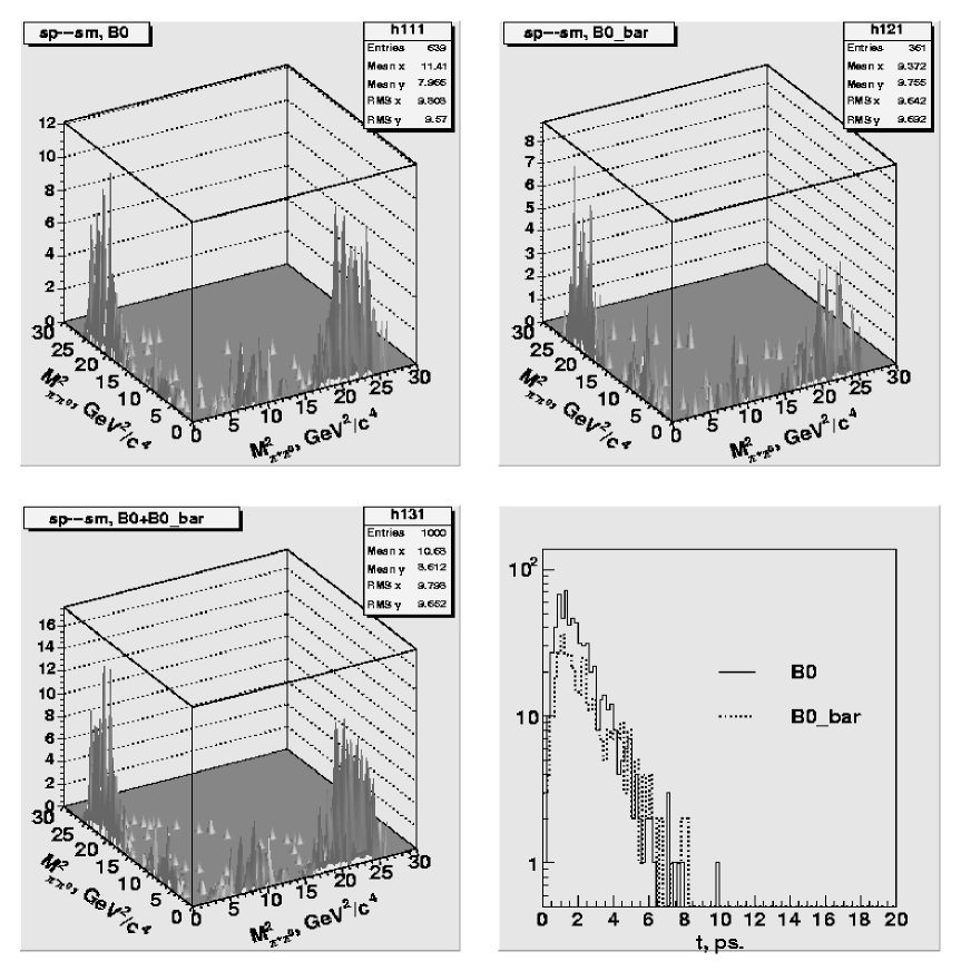
We have used two values for ฮฑ๐›ผ\alpha : ฮฑ=88โˆ˜๐›ผsuperscript88\alpha=88^{\circ} and ฮฑ=100โˆ˜๐›ผsuperscript100\alpha=100^{\circ}. For each case we have generated 500 independent trials, starting with different random numbers every time. Every trial contains 1000 signal events, 250 non-resonant background events and 250 resonant background events. This corresponds to one year (2ร—1072superscript1072\times 10^{7}s) of data taking. The background level was chosen based on the MonteCarlo studies described in section 5, for the case of of running at 396 ns bunch spacing (6 interactions per beam crossing), which would be BTeVโ€™s most challenging scenario. The Dalitz plot for one such sample is shown in Fig.ย 9.

Refer to caption

Figure 9: Dalitz-plot and proper time distribution for one trial of 1000 events for ฮฑ=88โˆ˜๐›ผsuperscript88\alpha=88^{\circ} (detector efficiency included).

To extract the parameters and the associated errors we have used an unbinned maximum likelihood fit. The likelihood over the full Dalitz domain is given by

โˆ’2โ€‹lโ€‹nโ€‹โ„’=โˆ’2โ€‹โˆ‘i=1NBd0lโ€‹nโ€‹โ„ฑi1+Rnโ€‹oโ€‹n+Rrโ€‹eโ€‹sโˆ’2โ€‹โˆ‘j=1NBยฏd0lโ€‹nโ€‹โ„ฑjยฏ1+Rnโ€‹oโ€‹n+Rrโ€‹eโ€‹s2๐‘™๐‘›โ„’2superscriptsubscript๐‘–1subscript๐‘subscriptsuperscript๐ต0๐‘‘๐‘™๐‘›subscriptโ„ฑ๐‘–1subscript๐‘…๐‘›๐‘œ๐‘›subscript๐‘…๐‘Ÿ๐‘’๐‘ 2superscriptsubscript๐‘—1subscript๐‘subscriptsuperscriptยฏ๐ต0๐‘‘๐‘™๐‘›ยฏsubscriptโ„ฑ๐‘—1subscript๐‘…๐‘›๐‘œ๐‘›subscript๐‘…๐‘Ÿ๐‘’๐‘ -2ln\mathcal{L}=-2\sum_{i=1}^{N_{B^{0}_{d}}}ln\frac{\mathcal{F}_{i}}{1+R_{non}+R_{res}}-2\sum_{j=1}^{N_{\overline{B}^{0}_{d}}}ln\frac{\overline{\mathcal{F}_{j}}}{1+R_{non}+R_{res}} (23)

where

โ„ฑisubscriptโ„ฑ๐‘–\displaystyle\mathcal{F}_{i} =\displaystyle= |๐’œ(si+,siโˆ’,ti,ฮฑ,..)|2๐’ฉ(ฮฑ,..)ร—ฮตโ€‹(si+,siโˆ’)+\displaystyle\frac{|\mathcal{A}(s^{+}_{i},s^{-}_{i},t_{i},\alpha,..)|^{2}}{\mathcal{N}(\alpha,..)}\times\varepsilon(s^{+}_{i},s^{-}_{i})+ (24)
+[Rnโ€‹oโ€‹nร—1๐’ฉt+Rrโ€‹eโ€‹sร—|โ„ฌโ€‹Wโ€‹(si+,siโˆ’)|2๐’ฉBโ€‹W]ร—ฮตโ€‹(si+,siโˆ’)delimited-[]subscript๐‘…๐‘›๐‘œ๐‘›1subscript๐’ฉ๐‘กsubscript๐‘…๐‘Ÿ๐‘’๐‘ superscriptโ„ฌ๐‘Šsubscriptsuperscript๐‘ ๐‘–subscriptsuperscript๐‘ ๐‘–2subscript๐’ฉ๐ต๐‘Š๐œ€subscriptsuperscript๐‘ ๐‘–subscriptsuperscript๐‘ ๐‘–\displaystyle+\left[R_{non}\times\frac{1}{\mathcal{N}_{t}}+R_{res}\times\frac{|{\mathcal{B}W}(s^{+}_{i},s^{-}_{i})|^{2}}{\mathcal{N}_{BW}}\right]\times\varepsilon(s^{+}_{i},s^{-}_{i})
โ„ฑยฏjsubscriptยฏโ„ฑ๐‘—\displaystyle\overline{\mathcal{F}}_{j} =\displaystyle= |๐’œยฏ(sj+,sjโˆ’,tj,ฮฑ,..)|2๐’ฉ(ฮฑ,..)ร—ฮตโ€‹(sj+,sjโˆ’)+\displaystyle\frac{|\overline{\mathcal{A}}(s^{+}_{j},s^{-}_{j},t_{j},\alpha,..)|^{2}}{\mathcal{N}(\alpha,..)}\times\varepsilon(s^{+}_{j},s^{-}_{j})+ (25)
+[Rnโ€‹oโ€‹nร—1๐’ฉt+Rrโ€‹eโ€‹sร—|โ„ฌโ€‹Wโ€‹(sj+,sjโˆ’)|2๐’ฉBโ€‹W]ร—ฮตโ€‹(sj+,sjโˆ’)delimited-[]subscript๐‘…๐‘›๐‘œ๐‘›1subscript๐’ฉ๐‘กsubscript๐‘…๐‘Ÿ๐‘’๐‘ superscriptโ„ฌ๐‘Šsubscriptsuperscript๐‘ ๐‘—subscriptsuperscript๐‘ ๐‘—2subscript๐’ฉ๐ต๐‘Š๐œ€subscriptsuperscript๐‘ ๐‘—subscriptsuperscript๐‘ ๐‘—\displaystyle+\left[R_{non}\times\frac{1}{\mathcal{N}_{t}}+R_{res}\times\frac{|{\mathcal{B}W}(s^{+}_{j},s^{-}_{j})|^{2}}{\mathcal{N}_{BW}}\right]\times\varepsilon(s^{+}_{j},s^{-}_{j})

Here sj+=(mฯ€++mฯ€0)j2subscriptsuperscript๐‘ ๐‘—subscriptsuperscriptsubscript๐‘šsuperscript๐œ‹subscript๐‘šsuperscript๐œ‹02๐‘—s^{+}_{j}=(m_{\pi^{+}}+m_{\pi^{0}})^{2}_{j} and sjโˆ’=(mฯ€โˆ’+mฯ€0)j2subscriptsuperscript๐‘ ๐‘—subscriptsuperscriptsubscript๐‘šsuperscript๐œ‹subscript๐‘šsuperscript๐œ‹02๐‘—s^{-}_{j}=(m_{\pi^{-}}+m_{\pi^{0}})^{2}_{j} are two Dalitz plot variables for the j๐‘—j-th event. NBd0subscript๐‘subscriptsuperscript๐ต0๐‘‘N_{B^{0}_{d}} and NBยฏd0subscript๐‘subscriptsuperscriptยฏ๐ต0๐‘‘N_{\overline{B}^{0}_{d}} are the total number of the Bd0subscriptsuperscript๐ต0๐‘‘B^{0}_{d} and Bยฏd0subscriptsuperscriptยฏ๐ต0๐‘‘\overline{B}^{0}_{d} events. The normalization ๐’ฉ=(|๐’œ|2+|๐’œยฏ|2)ร—ฮต๐’ฉsuperscript๐’œ2superscriptยฏ๐’œ2๐œ€{\mathcal{N}}=(|{\mathcal{A}}|^{2}+|\overline{\mathcal{A}}|^{2})\times\varepsilon is integrated over the Dalitz plane and over the proper time and weighted by the detector efficiency. Rnโ€‹oโ€‹nsubscript๐‘…๐‘›๐‘œ๐‘›R_{non} and Rrโ€‹eโ€‹ssubscript๐‘…๐‘Ÿ๐‘’๐‘ R_{res} are defined as

Rnโ€‹oโ€‹n=Nnโ€‹oโ€‹nbโ€‹aโ€‹cโ€‹kNBd0+Bยฏd0sโ€‹iโ€‹gโ€‹nโ€‹aโ€‹lRrโ€‹eโ€‹s=Nrโ€‹eโ€‹sbโ€‹aโ€‹cโ€‹kNBd0+Bยฏd0sโ€‹iโ€‹gโ€‹nโ€‹aโ€‹lformulae-sequencesubscript๐‘…๐‘›๐‘œ๐‘›subscriptsuperscript๐‘๐‘๐‘Ž๐‘๐‘˜๐‘›๐‘œ๐‘›subscriptsuperscript๐‘๐‘ ๐‘–๐‘”๐‘›๐‘Ž๐‘™subscriptsuperscript๐ต0๐‘‘subscriptsuperscriptยฏ๐ต0๐‘‘subscript๐‘…๐‘Ÿ๐‘’๐‘ subscriptsuperscript๐‘๐‘๐‘Ž๐‘๐‘˜๐‘Ÿ๐‘’๐‘ subscriptsuperscript๐‘๐‘ ๐‘–๐‘”๐‘›๐‘Ž๐‘™subscriptsuperscript๐ต0๐‘‘subscriptsuperscriptยฏ๐ต0๐‘‘R_{non}=\frac{N^{back}_{non}}{N^{signal}_{B^{0}_{d}+\overline{B}^{0}_{d}}}\qquad R_{res}=\frac{N^{back}_{res}}{N^{signal}_{B^{0}_{d}+\overline{B}^{0}_{d}}} (26)

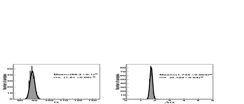
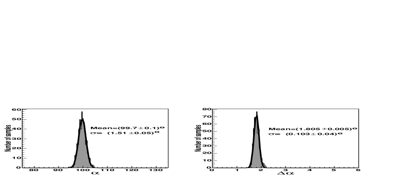
The fit has been performed for 500 samples, for each input value of ฮฑ=88โˆ˜๐›ผsuperscript88\alpha=88^{\circ} and ฮฑ=100โˆ˜๐›ผsuperscript100\alpha=100^{\circ}, to confirm the stability of the procedure. The results of the fit value for ฮฑ๐›ผ\alpha (right) and its deviation from the input value (left) are presented in Fig.ย 10(b), for the input values of ฮฑ=88โˆ˜๐›ผsuperscript88\alpha=88^{\circ} (Sample 1, Fig.ย 10(b)a) and ฮฑ=100โˆ˜๐›ผsuperscript100\alpha=100^{\circ} (Sample 2, Fig.ย 10(b)b), respectively. We measured ฮฑ=(88.3ยฑ1.6)โˆ˜๐›ผsuperscriptplus-or-minus88.31.6\alpha=(88.3\pm 1.6)^{\circ} and ฮ”โ€‹ฮฑ=(1.7ยฑ0.09)โˆ˜ฮ”๐›ผsuperscriptplus-or-minus1.70.09\Delta\alpha=(1.7\pm 0.09)^{\circ} for Sample 1 and ฮฑ=(99.7ยฑ1.5)โˆ˜๐›ผsuperscriptplus-or-minus99.71.5\alpha=(99.7\pm 1.5)^{\circ} and ฮ”โ€‹ฮฑ=(1.8ยฑ0.1)โˆ˜ฮ”๐›ผsuperscriptplus-or-minus1.80.1\Delta\alpha=(1.8\pm 0.1)^{\circ} for Sample 2, which is in good agreement with the input parameters.

These results have been obtained for ideal tagging. We have also made fits for different errors in the tagging dilution factor. The results are presented in Tableย 4 in the range from almost ideal ฯƒdโ€‹iโ€‹l=2subscript๐œŽ๐‘‘๐‘–๐‘™2\sigma_{dil}=2% to the very conservative ฯƒdโ€‹iโ€‹l=25subscript๐œŽ๐‘‘๐‘–๐‘™25\sigma_{dil}=25%. The displacements can be considered as systematic errors and should be summed with the ideal tagging error in quadrature. Assuming that the error in the tagging dilution factor in BTeV would have been 10-15%, we estimate the accuracy in measuring ฮฑ๐›ผ\alpha at (1.8โˆ’2.3)โˆ˜superscript1.82.3(1.8-2.3)^{\circ} for ฮฑ=88โˆ˜๐›ผsuperscript88\alpha=88^{\circ} and (3.4โˆ’4.7)โˆ˜superscript3.44.7(3.4-4.7)^{\circ} for ฮฑ=100โˆ˜๐›ผsuperscript100\alpha=100^{\circ}. We consider the most conservative case, a 15% error on the dilution factor for ฮฑ=100โˆ˜๐›ผsuperscript100\alpha=100^{\circ}, and conclude that BTeV could measure ฮฑ๐›ผ\alpha with the accuracy of better that 5โˆ˜superscript55^{\circ} in one year of operation.

Refer to caption
(a) Input value ฮฑ=88โˆ˜๐›ผsuperscript88\alpha=88^{\circ}
Refer to caption
(b) Input value ฮฑ=100โˆ˜๐›ผsuperscript100\alpha=100^{\circ}
Figure 10: Accuracy in determining ฮฑ๐›ผ\alpha : fit value of ฮฑ๐›ผ\alpha and deviation from input value (ฮฑiโ€‹nโ€‹pโ€‹uโ€‹tโˆ’ฮฑfโ€‹iโ€‹t)subscript๐›ผ๐‘–๐‘›๐‘๐‘ข๐‘กsubscript๐›ผ๐‘“๐‘–๐‘ก(\alpha_{input}-\alpha_{fit})

.

Table 4: The change (in degrees) of the value of the ฮฑ๐›ผ\alpha coming out of the likelihood fit at different errors in the tagging dilution factor (in %).
ฯƒdโ€‹iโ€‹lsubscript๐œŽ๐‘‘๐‘–๐‘™\sigma_{dil},%
input ฮฑ๐›ผ\alpha, degrees 2 5 10 15 20 25
additional displacement, degrees
88 +1.0 +0.4 -0.6 -1.6 -2.7 -3.9
100 -0.9 -1.6 -2.9 -4.3 -5.8 -7.2

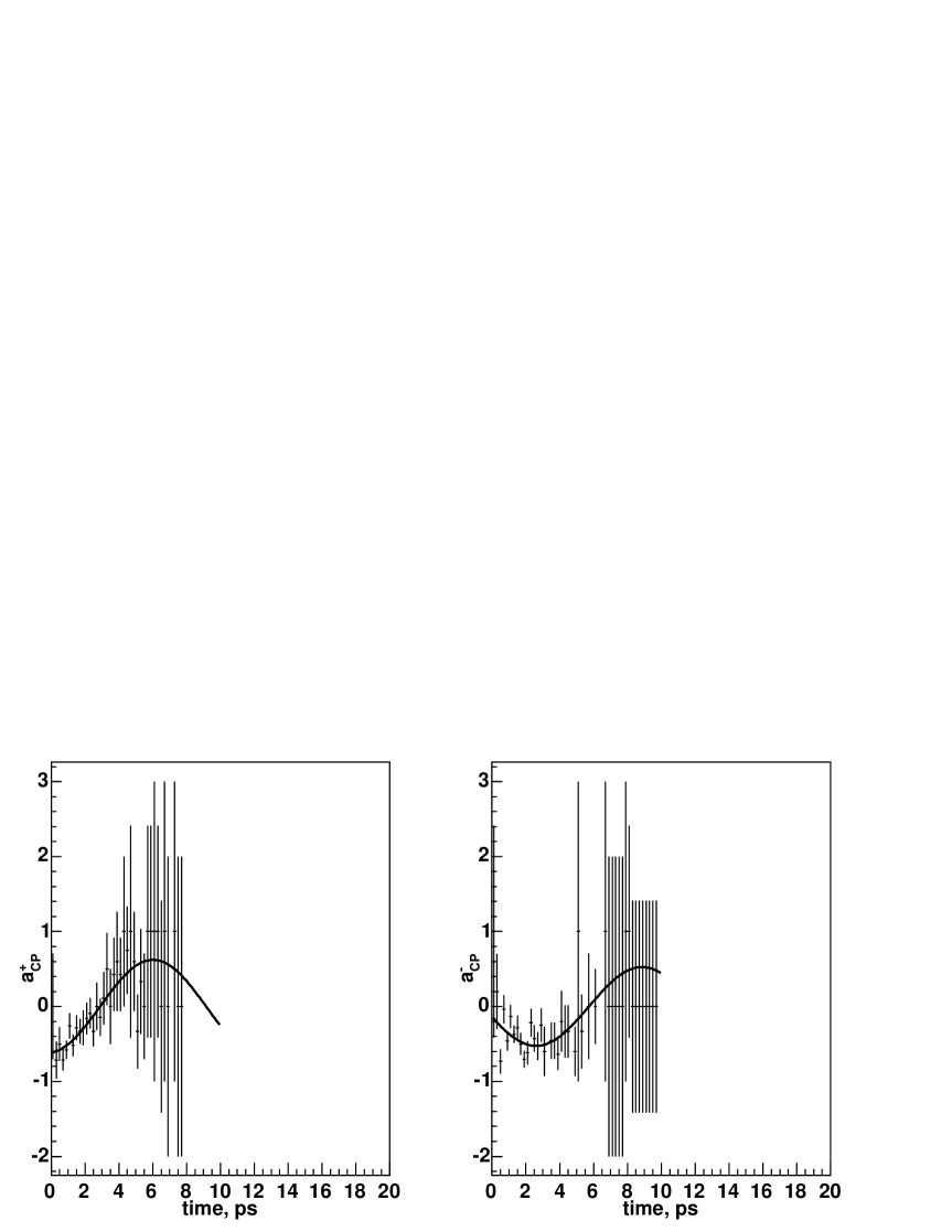
In order to ensure that our event generation model is correct (see eq.ย 17-20) we have integrated eq.ย 23 over the Dalitz-plot domain, so that only the proper time dependence of the B๐ตB-meson decay rate is left. We fit the data with the assumption of the time-dependent CP asymmetry of the B๐ตB-meson decay as expressed in eq.ย 16. The CP asymmetries acโ€‹p+superscriptsubscript๐‘Ž๐‘๐‘a_{cp}^{+} for ฯ+โ€‹ฯ€โˆ’superscript๐œŒsuperscript๐œ‹\rho^{+}\pi^{-} and acโ€‹pโˆ’superscriptsubscript๐‘Ž๐‘๐‘a_{cp}^{-} for ฯโˆ’โ€‹ฯ€+superscript๐œŒsuperscript๐œ‹\rho^{-}\pi^{+} (see eq.ย 17) are shown in Fig.ย 11 : the solid curves represent the fit results. The results obtained for the parameters in eq.ย 17 are :

Sฯโ€‹ฯ€=โˆ’0.22ยฑ0.06โ€‹(โˆ’0.15)subscript๐‘†๐œŒ๐œ‹plus-or-minus0.220.060.15S_{\rho\pi}=-0.22\pm 0.06(-0.15) (27)
ฮ”โ€‹Sฯโ€‹ฯ€=0.29ยฑ0.06โ€‹(0.33)ฮ”subscript๐‘†๐œŒ๐œ‹plus-or-minus0.290.060.33\Delta S_{\rho\pi}=0.29\pm 0.06(0.33) (28)
Cฯโ€‹ฯ€=0.38ยฑ0.05โ€‹(0.34)subscript๐ถ๐œŒ๐œ‹plus-or-minus0.380.050.34C_{\rho\pi}=0.38\pm 0.05(0.34) (29)
ฮ”โ€‹Cฯโ€‹ฯ€=0.24ยฑ0.05โ€‹(0.23)ฮ”subscript๐ถ๐œŒ๐œ‹plus-or-minus0.240.050.23\Delta C_{\rho\pi}=0.24\pm 0.05(0.23) (30)

where the numbers in parentheses represent the input to the simulation.

The results of the fit are in good agreement with the input values used in the Monte Carlo simulation. This justifies the validity of the model we used to extract ฮฑ๐›ผ\alpha and demonstrates that these important parameters could have been measured with the accuracy of 0.05-0.06 in one year of BTeV operation. As one can see in Tableย 3, up until now these values are known only crudely.
Refer to caption

Figure 11: CP-asymmetries acโ€‹p+superscriptsubscript๐‘Ž๐‘๐‘a_{cp}^{+} for ฯ+โ€‹ฯ€โˆ’superscript๐œŒsuperscript๐œ‹\rho^{+}\pi^{-} and acโ€‹pโˆ’superscriptsubscript๐‘Ž๐‘๐‘a_{cp}^{-} for ฯโˆ’โ€‹ฯ€+superscript๐œŒsuperscript๐œ‹\rho^{-}\pi^{+}. The solid curves represent the fit.

8 Conclusions

Physics simulations of the decay Bโ†’ฯโ€‹ฯ€โ†’๐ต๐œŒ๐œ‹B\to\rho\pi for the BTeV project at Fermilab has been performed. The main idea was to estimate the expected accuracy in extracting the angle ฮฑ๐›ผ\alpha of the UT.

To calculate the signal-to-background ratio for the decay of interest, 2ร—1072superscript1072\times 10^{7} background events were simulated and processed through the full detector simulation based on Geant3 package. Using the excellent electromagnetic calorimeter based on Lead Tungstate crystals, the Boโ†’ฯ+โ€‹ฯ€โˆ’โ†’superscript๐ต๐‘œsuperscript๐œŒsuperscript๐œ‹B^{o}\to\rho^{+}\pi^{-} decay the signal-to-background ratio is estimate at 4:1 or 2:1, for 132 ns or 396 ns beam crossing intervals, respectively.

A phenomenological analysis has been made for the possible values of tree and penguin amplitudes and phases for the process of interest, based on a global fit with SU(3)-flavor asymmetry for Bโ†’ฯโ€‹ฯ€โ†’๐ต๐œŒ๐œ‹B\to\rho\pi, Bโ†’Kโˆ—โ€‹ฯ€โ†’๐ตsuperscript๐พ๐œ‹B\to K^{*}\pi and Bโ†’ฯโ€‹Kโ†’๐ต๐œŒ๐พB\to\rho K. The latest experimental data from BaBar and BELLE were used in this analysis.

Dalitz-plot analysis of the Bโ†’ฯโ€‹ฯ€โ†’๐ต๐œŒ๐œ‹B\to\rho\pi decay with input from the phenomenological analysis has been presented. It has been shown that in one year of data taking BTeV could achieve the accuracy better than 5โˆ˜superscript55^{\circ} on the angle ฮฑ๐›ผ\alpha.

The interference between tree and penguin diagrams can be exploited by measuring the time dependent CP violating effects in the Bโ†’ฯโ€‹ฯ€โ†’๐ต๐œŒ๐œ‹B\to\rho\pi decays. In this paper it has been found that mixing-induced CP violation parameter Sฯโ€‹ฯ€subscript๐‘†๐œŒ๐œ‹S_{\rho\pi} and flavor-dependent direct CP violating parameter Cฯโ€‹ฯ€subscript๐ถ๐œŒ๐œ‹C_{\rho\pi} could be measured with the accuracy of 0.05-0.06.

9 Acknowledgments.

This work was partially supported by the U.S. National Science Foundation and the Department of Energy and the Russian Foundation for Basic Research grant 02-02-39008. We thank Alexander Bondar, Olivier Deschamps and Daniele Pedrini for fruitfull discussions.

References

  • [1] P. Langacker, โ€œCP Violation and Cosmology,โ€ in CP Violation, ed. C. Jarlskog, World Scientific, Singapore p 552 (1989).
  • [2] N. Cabibbo, Phys. Rev. Lett. 10, 531 (1963); M. Kobayashi and K.ย Maskawa, Prog. Theor. Phys. 49, 652 (1973);
  • [3] A.Bevan, โ€˜โ€™Measurements of sโ€‹iโ€‹nโ€‹2โ€‹ฮฑ/ฯ•2๐‘ ๐‘–๐‘›2๐›ผsubscriptitalic-ฯ•2sin2\alpha/\phi_{2} from Bโ†’ฯ€โ€‹ฯ€,ฯโ€‹ฯ€โ†’๐ต๐œ‹๐œ‹๐œŒ๐œ‹B\to\pi\pi,\rho\pi and ฯโ€‹ฯ๐œŒ๐œŒ\rho\rho modesโ€, hep-ex/0411090
  • [4] A.Kulyavtsev et al., Proposal for an Experiment to Measure Mixing, CP Violation and Rare Decays in Charm and Beauty Particle Decays at the Fermilab Collider - BTeV, May 2000;
    G.Y.Drobychev et al., Update to Proposal for an Experiment to Measure Mixing, CP Violation and Rare Decays in Charm and Beauty Particle Decays at the Fermilab Collider - BTeV, March 2002.
  • [5] A.ย E. Snyder and H.ย R. Quinn. โ€˜โ€™Measuring cp asymmetry in b โ†’โ†’\to rho pi decays without ambiguitiesโ€. Phys. Rev., D48:2139โ€“2144, 1993.
  • [6] L. Wolfenstein, Phys. Rev. Lett. 51, 1945 (1983).
  • [7] S. Stone, โ€œProspects For B-Physics In The Next Decade,โ€ in Techniques and Concepts of High-Energy Physics IX, ed. by T. Ferbel, NATO ASI Series, Plenum, NY (1996).
  • [8] M. Artuso, โ€œFlavour Physics: The Questions, The Clues and the Challenges,โ€ in proceedings of the Int. Europhysics Conf. on High Energy Physics, Tampere, Finland, July, 1999, ed. K. Huitu, H. Kurki-Suonio and J. Maalampi, Inst. of Physics Publishing (Bristol) p91 (hep-ph/9911347).
  • [9] BABAR Collaboration, B.Aubert at al., hep-ex/0408127
  • [10] BELLE Collaboration, K.Abe et al., Phys.Rev. D71, 072003 (2005), hep-ex/0408111.
  • [11] The Heavy Flavor Averaging Group, http://www.slac.stanford.edu/xorg/hfag/ (Summer 2003 and Winter 2004 averages)
  • [12] M. Gronau, Phys. Rev. Lett. 63, 1451 (1989); M. Gronau and D. London, Phys. Rev. Lett. 65, 3381 (1990).
  • [13] The theoretical accuracy of this approach is limited by electroweak penguins, that are expected to be rather small in this case. In principle, they can be taken into account, as pointed out by A. J. Buras and R. Fleischer, Eur. Phys. J. C11, 93 (1999) (hep-ph/9810260), and also by M. Gronau, D. Pirjol and T-M. Yan, Phys. Rev. D 60, 034021 (1999) (hep-ph/9810482).
  • [14] H. J. Lipkin, Y. Nir, H. R. Quinn, and A. Snyder, Phys. Rev. D44, 1454 (1991)
  • [15] BABAR Collaboration, B.Aubert et al., hep-ex/0408099 (2004); BABAR Collaboration, B.Aubert et al., hep-ex/0503049 (2005)
  • [16] F. Abe et al.., โ€œMeasurement of the B๐ตB Meson Differential Cross-Section in pโ€‹pยฏ๐‘ยฏ๐‘p\overline{p} collisions at s๐‘ \sqrt{s} = 1.8 TeV,โ€ CDF/PUB/BOTTOM/PUBLIC/3759 submitted to ICHEP โ€™96 and references therein; F. Abe et al.., Phys. Rev. Lett. 75, 1451 (1995).
  • [17] R. Abbott et al.., โ€œThe bโ€‹bยฏ๐‘ยฏ๐‘b\overline{b} Production Cross Section and Angular Correlations in pโ€‹pยฏ๐‘ยฏ๐‘p\overline{p} collisions at s๐‘ \sqrt{s} = 1.8 TeV,โ€ FERMILAB-Pub-99/144-E; S. Abachi et al., Phys. Rev. Lett. 74, 3548 (1995).
  • [18] M. Mangano, P. Nason and G. Ridolfi, Nucl. Phys. B 373, 295 (1992).
  • [19] I. Redondo, โ€œZEUS Results on Charm in DIS as an Indication of Beam Drag Effects,โ€ and E. Norrbin and T. Sjostrand, โ€œDrag Effects in Charm Photoproduction,โ€ both in Proceedings of the workshop for Monte Carlo Generators for HERA Physics, 1998/99, ed. by A. T. Doyle et al., http://www.desy.de/ย heramc/proceedings/wg60.
  • [20] M. Artuso, โ€œExperimental Facilities for b-Quark Physics,โ€ in B๐ตB Decays revised 2nd Edition, Ed. S. Stone, World Scientific, Singapore (1994).
  • [21] F. Abe et al.., Phys. Rev. D 53, 1051 (1996).
  • [22] GEANT: Cern Program Library Long Writeup W5013, http://wwwinfo.cern.ch/asdoc/geant_html3/geantall.html.
  • [23] M.ย Gronau and J.ย Zupan, arXiv:hep-ph/0407002.
  • [24] M.ย Beneke, G.ย Buchalla, M.ย Neubert and C.ย T.ย Sachrajda, Nucl.ย Phys.ย B 606, 245 (2001) [arXiv:hep-ph/0104110];
    M.ย Neubert, arXiv:hep-ph/0012204.
  • [25] M.ย Beneke and M.ย Neubert, Nucl.ย Phys.ย B 675, 333 (2003) [arXiv:hep-ph/0308039].
  • [26] J.ย Charles et al. [CKMfitter Group Collaboration], arXiv:hep-ph/0406184.
  • [27] R.ย Aleksan et al. Nucl. Phys. 361B, 141, 1991