The scattering of muons in low Z materials.

Abstract

This paper presents the measurement of the scattering of 172 MeV/c muons in assorted materials, including liquid hydrogen, motivated by the need to understand ionisation cooling for muon acceleration.

Data are compared with predictions from the GEANT 4 simulation code and this simulation is used to deconvolute detector effects. The scattering distributions obtained are compared with the Moliere theory of multiple scattering and, in the case of liquid hydrogen, with ELMS. With the exception of ELMS, none of the models are found to provide a good description of the data. The results suggest that ionisation cooling will work better than would be predicted by GEANT 4.7.0p01.

1 Introduction

The storage of intense muon beams is required for the construction of a Neutrino Factory or muon collider. The ionisation cooling techniqueref:cooling is a leading contender to maximise the intensities for the Neutrino Factory and it is even more likely to be used at a muon collider. This technique relies upon the cooling effect of dE/dx losses in low Z materials coupled with R.F. acceleration to reduce the emittance of a beam. Multiple scattering in the material heats the beam and the overall cooling is thereby reduced. It is therefore important to confirm the theoretical understanding and computational implementations of multiple scattering of muons of around 200 MeV/c. There is no published measurement of muon scattering in this region, and furthermore data on electron scattering with similar $\beta$ref:andrievsky suggest an excess in the tails compared with predictions from Moliere theoryref:moliere , especially for low $Z$ materials. This was first observed in ref. ref:fernow .

Many problems involving multiple scattering have employed GEANT 4 ref:g4 to evaluate the effects. A new model of scattering, ELMSref:elms , has recently become available. This is a return to electromagnetic first principles, but often uses numerical integration rather than closed-form approximate integrals.

The MuScat experiment was accepted by TRIUMF in 1999 to run in the M11 muon beam-line, and an engineering run took place in summer 2000. A new scintillating fibre tracker was built for the physics run. The data presented here were collected in April and May 2003, in the M20 muon beam-line in TRIUMF.

Section 2 contains a description of the principle and technology of the MuScat experiment. This is followed in sections  3, 4 and 5 by details of the performance of the tracker, calorimeter and scintillator subsystems. The beam properties are described in section 6. These descriptions are accompanied by discussion of the GEANT 4 model which was used to deconvolute the detector effects, a process discussed in section 7. The data are presented in section 8, and conclusions can be found in section 9.

The detector performance has been modelled using GEANT 4.7.0p01. This toolkit was used to make a complete description of the geometry shown in figure 1. Considerable attention has been attached to the simulation of the collimator system and the fibre tracker, which are critical to the experiment and whose performances are sufficiently complex that they are hard to extract from the data alone.

2 The Experimental Apparatus

The technique of the MuScat experiment was to prepare a narrow collinear muon beam by collimation, and to use it to illuminate a variety of target materials. The position of the outgoing particles was measured after travelling a sufficient distance that the position and angle were highly correlated.

Figure 1: The MuScat detector, from the GEANT 4 model.

The key components are the collimation system, a wheel with a selection of solid targets and an optional liquid hydrogen (LH₂) vessel, a scintillating fibre tracker, and the trigger scintillators. In addition to these the TINA (TRIUMF Iodide of Sodium) calorimeterref:tina was useful to help understand the system. There were also some extra scintillators employed as veto counters.

The passive components have been implemented in a GEANT 4 model in a simplified manner, sufficient to simulate the materials which would affect the observed scattering distributions. The position of many externally visible components were checked with a precision of a few mm in the M20 beam-line in TRIUMF, and no deviations found. The position of the target wheel is known from the engineering drawings. The locations of the scintillators and the TINA calorimeter are known from the measurements.

The coordinate system chosen is that z is defined approximately by the beam direction, y is vertical and x is horizontal so as to define a right handed coordinate system. Since the collimator slits are narrow in the vertical direction, the y coordinate of a muon is the measure of its scattering. The precise definition of the $z$ axis is that that the first two detector planes are both centred on $x=y=0$.

2.1 The M20 beam-line

The experiment used the M20 beam-line at TRIUMF. The extracted proton beam from the cyclotron interacted in a target and produced pions at a production angle of 55 degrees. The beam-line had a muon decay channel consisting of two dipoles with quadrupole focusing. The beam-line was tuned to optimise the capture of high momentum muons from forward pion decays. The mean beam momentum was 172$\pm$2.0 MeV/c and the accepted momentum bite was approximately 1 MeV/c. The beam delivered to the experiment consisted of muons with a small pion background, but a mixed beam could be produced, as described later in the discussion of the time of flight system. The trigger rate was 80 particles/sec; the particle rate incident on the first scintillator, before collimation, was three orders of magnitude larger. The spot size at the first collimator was 50 mm in diameter.

2.2 The Collimator

Figure 2: The second collimator piece, made of 160 mm of lead. On the left is the computer model, and on the right the two interlocking pieces of lead used to construct it.

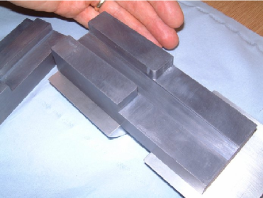
The collimator system consisted of two lead blocks with slits in them, augmented by other active and passive collimators. The accepted particles had to pass through both slits. This defined a beam which was narrow in one direction, vertically, but much broader in the other to maintain rate. The upstream lead block was 40 mm thick, with a simple slit, 20 mm by 2 mm. The second block, shown in figure 2, had a trapezoidal slit, 12.8 mm by 2.0 mm at the upstream end, expanding to 20.0 mm by 2.88 mm at the downstream end. The collimator blocks were each made from two interlocking pieces of lead, with the lower one fixed to two steel rods by aluminium supports. The distance between the outer faces of the collimators was 963 mm.

The system was behind a shield wall; 8 cm thick steel with a 4 by 3 cm opening aligned with the lead collimators. There were also eight auxiliary collimators, made from lead discs 20 mm thick and with 20 mm diameter openings, which were mounted on the steel rods between the two main collimators. They were intended to intercept any particle which might have scattered in the jaws of the first collimator and then missed the second one entirely. They were designed so particles scattered from them could not pass through the slit in the final collimator without another interaction. The entire tube was wrapped in lead sheet to a thickness of 6 mm. This ensures that all muons reaching the tracker have passed through the entire collimator system.

Finally, the downstream passive lead collimator was supplemented with two scintillators, 3 mm by 3 mm by 30 mm. These were positioned just at the front face of the collimator, above and below the slit. They were designed to record particles which might otherwise have hit the lead and then emerged into the slit with a large scattering and energy loss. They were read-out by 7 of the clear 1 mm fibres used for the Sci-Fi tracker. The fibres were attached to each end and taken to a photomultiplier tube (PMT).

Figure 3: The distribution of particles at detector plane 1 in data and simulation for no target. The error bars include systematic error estimates. The large error bar just to the right of the peak includes the effect of possible misalignment.

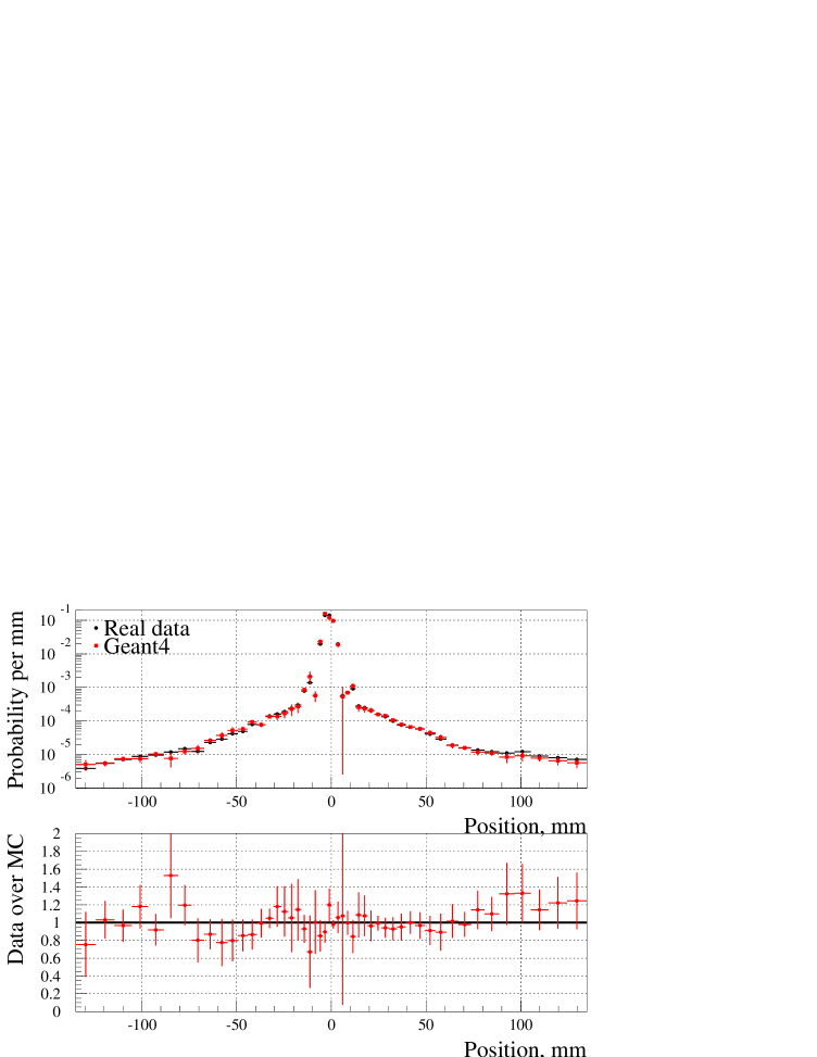
The width of the collimated beam must be well simulated, and unfortunately this is not the case with the assumption of a perfect geometry. The apparent slit width and also the observed tails are both wider in data than in the simulation. The only credible way to increase the collimated beam width is to hypothesise that the second collimator was not perfectly closed. It was constructed as two blocks of lead which dovetail neatly and firmly but are not attached together. The lower block was held firmly to the rails, and the whole assembly is prevented from rotating by a grub screw through the collimator tube attached to the top lead block. If the system was somehow pressured after or during installation the grub screw could pull the top lead back, widening the jaw. The simulated distribution of particles through the expanded collimator assumption is shown in figure 3, and this is used hereafter.

This is unfortunate, as not only does the central distribution widen but the inner faces of the collimator can become directly exposed to incident particles, allowing scattering from them. These tails are indeed observed. The energy distribution of the tail particles, as measured in TINA, is consistent with what would be expected if this is the correct explanation. The size of the movement is small. The best representation of the observed data is obtained if the jaw is opened from 2.0 mm to 2.48 mm.

2.3 The target system

There were two separate target systems: a wheel with a choice of solid targets and a vessel for liquid hydrogen. The target wheel was controlled by a stepper motor, and presented a choice of twelve target positions to the beam. The position was monitored by an optical LED system which allowed readout of the target number and a confirmation that the position was exactly correct. Table 1 shows the targets used, and the number of events selected for analysis from each. The density and radiation length, X₀, are also shown.

No.	Material	Thickness, mm	Density, g/cc	X0, %	Events
0	Lithium	12.78	0.53	0.82	805239
1	Lithium	6.43	0.53	0.41	1224756
2	Lithium	6.40	0.53	0.41	882449
3	Lithium	12.72	0.53	0.81	1215336
4	Beryllium	0.98	1.85	0.28	500766
5	Beryllium	3.73	1.85	1.06	1186528
6	CH2	4.74	0.93	0.99	802426
7	Carbon	2.50	1.69	1.53	801899
8	Aluminium	1.50	2.70	1.69	1201280
9	None	-	-	-	2259476
10	Iron	0.24	7.86	0.82	845020
11	Iron	5.05	7.86	28.68	1225435
	Empty H2	109.0	-	-	2694511
	H2	109.0	0.0755	1.31	2267683
	Empty H2	159.0	-	-	812730
	H2	159.0	0.0755	1.90	1127045

Table 1: The targets, and the number of data events selected for each.

The LH₂ vessel was crucial to the experiment, because scattering in liquid hydrogen was the most important goal. This was designed and built by the cryogenic targets group at TRIUMF. There is a contribution to the scattering from the containing windows, and therefore it it is essential to minimise and measure this accurately. The vessel could be filled with liquid or gaseous hydrogen, and the measured distributions with gaseous hydrogen are used to characterise the windows. The temperature remained between 15 and 23 K for these cycles, and there was always a slight overpressure.

The vessel was 150 mm by 100 mm by 100 mm. The 150 mm length was bored with an 8 cm diameter hole, and an identical hole was made through from one side. These were capped by four identical windows in the sides and ends, so that by rotating it a choice of hydrogen thicknesses was presented. The windows bulged by 4.5 mm, with an estimated error of 0.3 mm, making the total length 109.0$\pm$0.6 mm or 159.0$\pm$0.6 mm. They were made from mylar, 5 thousands of an inch thick, wrapped in 6 layers of super-insulation.

3 The Sci-Fi tracker

The scintillating fibre (Sci-Fi) tracker comprised three double fibre planes, read out by twenty-four HPK multi-anode PMTs ref:PMT . The planes were about 1100 mm from the target. The first and second planes were mounted together, which means the active elements were displaced by 50 mm. While for the third plane the displacement was 66.9 mm.

Figure 4: The layout of the scintillating fibres. Each plane consists of both horizontal and vertical fibres, overlapping in two rows to give complete coverage. In each row the distance between fibre centres was 1.17 mm and the distance between the rows was 1.17 mm. They are potted in black epoxy.

The double planes consisted of two planes (each constructed as shown in figure 4), one comprising 512 horizontal fibres and the other the same number of vertical fibres. They have a pitch of 0.585 mm, covering 300 mm². The fibre diameter was 1 mm, including the outer 4% cladding. They were arranged in double rows, as in figure 4. They were held in a Delrin frame, 350 mm square with a 300 mm square central area. 2048 holes were drilled with a CNC machine to define the locations of the two ends of each fibre. The fibres were held under tension and potted in black epoxy. Finally the ends of the fibres were cut.

Figure 5: The physical arrangement of the Sci-Fi tracker. The left hand figure shows one plane mounted inside the vessel. The black frame at the top encloses the scintillating fibres, and the clear routing fibre bundle can be seen. The right hand figure shows the front faces of the fibre bundles, with a PMT mounted onto one of them.

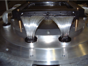
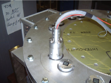
Each double plane had four Delrin edge connectors, made in a similar manner, and drilled in one operation with the frame so that the holes matched. This can be seen in figure 5 (left). Into each of these connectors were potted 512 double-clad 1 mm radius clear fibres which were to guide the light to photo-multipliers. This was done in two groups of 256, and the far ends of the fibres, after about 300 mm, were arranged into a square 16 by 16. These were potted in an aluminium former which was to also act as a vacuum seal for the detector vessel. The natural tendency of the fibres to close-pack made this construction difficult, and the edge fibres were not always perfectly placed. The best bundles were selected for the first detector and for measuring y. The 16 mm square fibre bundles presented on the outside of the pressure vessel were connected to the 16-anode PMTs, as shown in figure 5 (right). The readout was done with a custom-made sample and hold system, which provided a stable, low-noise readout for the system.

Each set of 256 fibres is read out at both ends. One end of the fibres is read out by a PMT which measures the signals from 16 adjacent fibres in each of its (16) anodes. The other set of ends is distributed across the PMT surface so that each PMT anode reads every sixteenth fibre. In this way, one PMT is used to measure which group of 16 fibres has a signal and the other which fibre within the group. This multiplexing scheme can only work with a single charged particle present.

Simulation of the tracker was fairly complete. The light yield per fibre in the simulation was tuned to the data using the mean measured signal in identified hits using the thick iron target. For a few percent of fibres with low light yields this does not converge satisfactorily; for these the rate of hits is used instead. Cross-talk and signal shape were simulated due to the light spreading in the 1.5 mm glass at the front of the PMT, the photo-electrons jumping to other dynodes, a leaky dynode chain where an electron can skip a stage or move into the neighbouring chain and about one percent of electronic cross-talk.

Figure 6: Left: The number of ADC counts on every channel in data and simulation with the thick iron target. The peak at 600 is due to single photo-electrons. Right: The distribution of the number of fibres with a signal of over 0.2 photo-electrons observed in data and simulation.

The distribution of ADC counts recorded on all channels is in figure 6 (left). The pedestal is clearly visible, with a peak due to single photo-electrons at around 600 counts which was used to measure the gain. The upper edge is cut off by the saturation of the ADCs. The simulation includes these effects and shows reasonable agreement.

The distribution of the number of reconstructed fibres with signals in data and simulation is shown in figure 6 (right). The data has events with no fibres hit which are not reproduced by simulation. These are trigger accidental coincidences. There are also events with several times the normal number, which arise from multiple tracks. Both types of events are removed in analysis. The central region has a reasonable representation.

Figure 7: The distribution of particles at detector plane 1 in data and simulation when the thick iron target is in place.

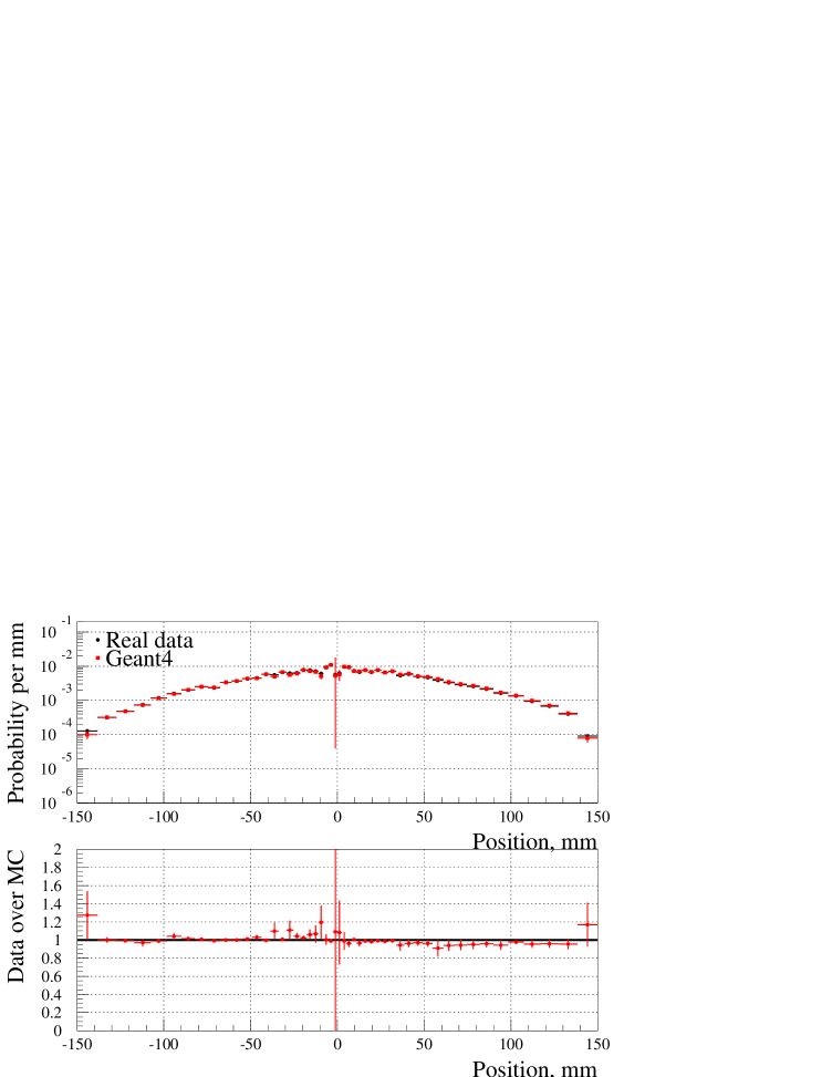
The recognition of a hit in the tracker depends upon the observation of at least one photon at either end, and as the average light yield is around four photons then any poor fibres with lower yields will have significant inefficiency. This is examined in figure 7, which shows the results for a thick iron target, of 28% X₀. The scattering distributions in this target are dominated by the central Gaussian core, and the simulations are therefore expected to be reliable. The purpose of this target is to illuminate the entire detector with tracks for use in alignment and efficiency studies. There is a distinct drop in efficiency at the very centre of the distribution, and also some structure at about -10 mm. The distribution is shown for the entire detector, and the agreement is well within 10% in most bins, with the centre and the edge bins showing differences around 20%. It seems that the simulation of the edges of the PMTs is somewhat defective, probably due to the difficulty of locating all the clear fibres in the correct places at the front of the PMT.

4 The TINA Calorimeter

An existing calorimeter from the TRIUMF Laboratory, ‘TINA’ref:tina , was used to understand the beam properties. This is a cylindrical sodium iodide calorimeter, 460 mm diameter and 510 mm long, split into two crystals in depth. It is read out using 7 PMTs on the back-face, one in the centre and the other six in a circular pattern around it. The calorimeter is contained in a metal blockhouse to reduce external backgrounds. This blockhouse has a small lip that overlaps the outer edge of the NaI by about 40 mm. The device has a measured energy resolution (fwhm) of 3.6% at 90 MeV for electrons, with an energy dependence of $E^{-0.55}$.

As TINA was too small to cover the complete angular acceptance of MuScat, it was mounted with the centre shifted upwards by 70 mm with respect to the axis of the experiment. This allowed a complete angular coverage in the positive y direction. In addition, the energy deposition was integrated over two time periods: tina_early, corresponding to 500 ns from the S1B trigger, and tina_total, corresponding to 10 $\mu$s from the trigger. In general, the first of these will have only the kinetic energy of the muon, while the second also contains the electron from the decay of the muon, which has come to rest in TINA

Figure 8: The tina_early ADC signal in the TINA calorimeter for events selected by timing cuts (see section 6.2) to be either mixed pion and muon events (left) or the muon sample used for analysis (right). A requirement on tina_total - tina_early has been made so that the muon decay is known to occur after the tina_early gate closed, but a small decay tail can still be seen. The peak at 245 ADC counts is the pedestal.

The performance of TINA is illustrated by figure 8. The pedestal is at 245 ADC counts. The left hand plot (pion sideband), shows the separation between pions and muon peaks. Decay electrons have been supressed as discussed in the caption. If this had not been done there would have been larger tails, and an additional 0.4% would have been assigned to the background. The TINA calorimeter was modelled in GEANT 4, but these simulations are not used in this analysis.

5 The Scintillators

There were seven instrumented plastic scintillators used in the experiment. Three of these made up the trigger system, and the other four were veto counters.

The trigger was provided by a logical and of two overlapped finger scintillators, 3 mm square in area and 30 mm long, known as S1A and S1B. These were mounted in front of the collimator to record particles before entering the system. They gave a precise timing signal, used for the time of flight measurements discussed later. This was taken in coincidence with the signal from a 330 mm square scintillator, referred to as S2, which was read out by two PMTs, top and bottom, whose results were combined as a logical or. S2 was placed after the Sci-Fi tracker and before TINA as shown in figure 1.

Two large area veto scintillators were butted together just in front of S1; one had a notch removed that corresponded approximately to S1. These are referred to as V1. The other two veto scintillators were bars 3 mm by 3 mm by 30 mm which were mounted on the front face of the second lead collimator, just above and just below the slot.

The common start for all the TDCs (Time to Digital Converters) in the experiment came from the S1B  scintillator. A delayed version of S1B  was then read by a TDC. This should have given a fixed time, but some events were several ns different and they were removed by offline selection. An additional signal from the cyclotron, repeated each 43 ns period, provided a useful timing reference.

The GEANT model included accurate descriptions of the geometry of the scintillator system. Electronic handling of the signals, in terms of pulse shaping, and discriminator threshold for the TDCs was included in an approximate way so that time-walk effects were reproduced.

In order to reproduce the data, the finger scintillators comprising the active collimators had to be positioned so that they overhung into the collimator gap slightly: the top by 190 $\mu$m and the bottom by 70 $\mu$m. This reinforces the idea that the collimator slot had somehow opened.

6 Beam properties

There has been no attempt to simulate the beam-line. However, the x distribution of the observed beam has a very small dependence upon the initial beam configuration, and for y it is totally negligible. The beam divergence is instead determined by multiple scattering in the S1A and S1B scintillators, which guarantees a minimum spread, followed by the collimation system which limits the maximum angle.

6.1 Beam momentum determination

Figure 9: The time of arrival of the beam cycle signal relative to the S1B scintillator for run 177, which was tuned to have a mixed particle content. The four lines guide the eye to pions, muons, protons and electrons. The open histogram is for all events that are in time on S1B  and the hashed area for events that meet a tighter requirement on S1B  within 0.25 ns of expected, which excludes protons. A double peak structure can be seen for the precise peaks; this is not understood.

A special run was taken with the momentum of the second dipole in the beam-line turned down by 2%. This meant that the forward muons normally accepted have a large contamination from other species. The presence of multiple particle types has been used to measure the beam momentum. The time of arrival of the cyclotron signal relative to S1B is shown in figure 9. The major peaks are at 500 (pions), 650 (muons), 750 (protons) and 900 (electrons). In general the fastest particles give the largest times, because what is measured is the arrival time of the cyclotron signal after S1B. In the case of protons, the velocity is only 0.2 c, and they arrive seven beam crossing periods late. The width in the electron and pion signals are similar, but the others are broader. For protons this is because the very low velocity leads to a much larger spread in time, while the muon arrival time depends upon the decay point. There is a distinct peak of muons which were produced before the first bending magnet.

Figure 10: Fitting the beam momentum from the observed peaks using the cyclotron signal. The negative of the arrival time of the cyclotron signal is plotted; for protons a point is shown both at the measured time and delayed by seven beam cycle periods.

The momentum of the beam has been estimated by fitting the arrival times of all four particle species. Three parameters are required for this: the time offset, (defined by the arrival time of a particle going at the speed of light), the length of the beam-line and the beam momentum. The results are shown in figure 10, where a momentum of 168.9 MeV/c is found and the four points are seen to be consistent. This run was taken with the final dipole field reduced by 2%, so under normal running conditions the beam momentum is 172$\pm$2 MeV/c.

The spread in momentum can be estimated by noting that it affects the velocity of pions but not electrons. The quadrature difference in width of the pion and electron peaks calculated as in figure 9 but after accounting for small time-walk effects gives the spread in momentum as being between 1.0 and 1.2 MeV/c.

6.2 Beam composition

The recorded sample under normal conditions has a large proportion of muons. This can be seen in figure 11. Protons are ranged out in the S1A  trigger, and not generally recorded. This figure shows a somewhat worse time resolution than in figure 9, which is not understood but was constant for the data used for the main analysis.

Figure 11: The time of arrival of the beam cycle signal relative to the S1B scintillator for run 290, an ordinary run with no target. The graph corresponds to events where the digitised time from S1B was correct. The section labelled $\mu$ contains those events used for the scattering analysis. The small peak to the right contains electrons. The resolution is slightly worse than in figure 9; this is not understood.

The muon fraction is further raised by demanding that the recorded time of the TOF signal is within the section labelled $\mu$ in the figure. The energy recorded in TINA for the subset of events within its acceptance is used to evaluate the purity of this sample. The left hand plot on figure 8 (pion sideband), has two large peaks due to pions (left) and muons (right). The distribution is fitted using two Gaussian distributions to determine the peak positions and widths. The relative amplitudes of these contributions are then fitted to the right-hand plot, where a 0.8% pion component is found. Some contribution to the second Gaussian comes from resolution tails, and therefore the pion contamination is almost certainly overestimated.

7 Analysis Method

7.1 Event Selection

The selection of events for analysis requires that they pass a number of selection criteria. Firstly the high voltage must have been nominal and the data-acquisition in a normal state. Then we require that the event was not taken during a period identified as having a problem with the time of flight system.

Next the number of reconstructed points on the first plane of the tracker is required to be one or two; more hits would make the position of the muon very ambiguous. Then the summed signal from the two internal veto scintillators had to be consistent with the pedestal, and the time from S1B within a few counts (0.2 ns) of nominal.

The hit with the largest light yield is taken as the estimated particle position at each detector plane. Finally, the positions of the hits on the first and second planes are required to be consistent with the hypothesis of a particle coming from the target. The second plane is about 4% further from the target, so it is required that 0.96 times the y position on the second plane be within 5 mm of the y position on the first plane. This procedure is simpler than performing a full track fit, and less dependent upon alignment systematics.

7.2 Deconvolution technique

It is possible to compare the distributions of hits at the first detector plane. However, the more fundamental quantity is the angle through which the particle scattered in the target, and the effects of beam width, efficiency, resolution etc. must be corrected for to see this. This deconvolution is done using the GEANT 4 simulation, with the following approximate formula:

$$\overline{D}=\overline{B}+\overline{D_{\pi}}+\overline{\overline{R}}\cdot\overline{\overline{\epsilon}}\cdot\overline{\Theta}$$ (1)

Where $\overline{D}$ is the observed position data, $\overline{B}$ a background of particles not passing through the target, $\overline{D_{\pi}}$ is the contamination from pions, $\overline{\overline{R}}$ is the response of the detector to a particle deflected through angle $\theta_{y}$, $\overline{\overline{\epsilon}}$ is the efficiency of the detector for particles deflected through angle $\theta_{y}$, and $\overline{\Theta}$ is the projected scattering distribution in the target.

The background, $\overline{B}$, is found from simulation as those muons which managed to meet the trigger conditions without passing through the target. There are typically 0.125% background events. The pion contamination, $\overline{D_{\pi}}$, is taken from the data pion sideband. The default value is 0.8% pions, and as the sideband is approximately 50% pions, a 1.6% admixture of the data sideband is added to the simulation.

The response and efficiency matrices, $\overline{\overline{R}}$ and $\overline{\overline{\epsilon}}$ are taken from simulation. The efficiency is found by running GEANT 4 twice. The first run is a simulation of the target only, illuminated by a monochromatic collinear beam of muons. This is used to find the true $\overline{\Theta}$ distribution in GEANT 4. The second run is the full simulation, including trigger and tracking acceptance cuts. The distribution $\overline{\Theta}$ for those muons accepted is calculated, and the ratio of these is $\overline{\overline{\epsilon}}$. In the above formula it is treated as a diagonal matrix. Finally, $\overline{\overline{R}}$ is filled as a 2D matrix, with each accepted simulated event being entered at a point given by its $\theta_{y}$ and the y position at the first measurement plane. It therefore gives the probability of a given measured position for each possible true deflection angle.

The equation is solved for $\overline{\Theta}$, imposing a requirement of symmetry about $\theta=0$, using Minuitref:Minuit , which also finds errors and correlations. It has been checked that the technique is mathematically correct, in that if given simulated data as an input the scattering distribution from that simulation is recovered.

This formalism does not explicitly include the effect of energy losses and scattering in the $X$ direction. The matrices $\overline{\overline{R}}$ and $\overline{\overline{\epsilon}}$ therefore depend on the simulation of multiple scattering and energy loss in the GEANT model. In particular, the probability that a particle completely misses the detector in the $X$ direction as a function of its $Y$ angle must be taken from simulation.

The problem of instabilities in the deconvolution has been dealt with by reducing the number of bins in the deconvoluted data, where 21 are used, compared to the raw data, which has 57. Furthermore the condition of symmetry is enforced in the fit, so there are essentially only 11 bins. Finally, the outermost bin in true scattering angle runs from 115 mrad to $\pi$, but is very weakly constrained by the data as the majority of events in this bin are not recorded. It also has a strong dependence on the simulated prediction of the fraction recorded. It is not shown in the plots which follow.

8 The results

8.1 Comparisons at detector level

Figure 12: The distribution of particles at detector plane 1 in data and simulation for the empty H₂ vessel in the 150 mm position.

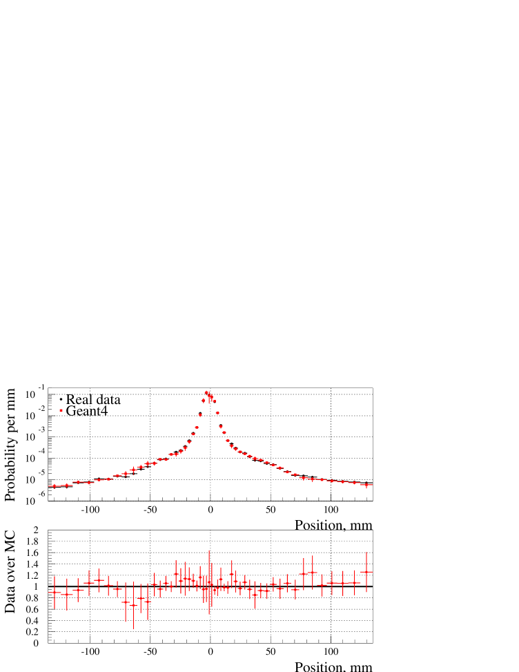
Data taken with no target, an empty hydrogen vessel or a very thick iron target are not of great intrinsic interest, but were necessary to understand the detector. The first, the bare collimator distribution, is shown in figure 3. The final results are based upon deconvoluting the data using the simulation, and so discrepancies here will translate into systematic errors on the results. In the case of hydrogen data, the equivalent of the bare collimator is the empty target vessel. The distributions obtained for this in data and simulation are showing in figure 12 for the case of the longer target configuration.

The error bars shown in these plots are statistical only for the data but are a combined statistical and systematic error on the simulation points. This systematic error explicitly includes the difference between these plots, and so by construction all ratios must be compatible with one to within one combined error.

The other control plot is figure 7, which shows the results for a thick iron target, of 28% X₀. The agreement is well within 10% in most bins, with the centre and the edge bins showing differences around 20%. As the edge bins have also got a large background subtraction, the region of the detector used for analysis and subsequent figures is restricted to the central 270 mm.

Figure 13: The distribution of particles at detector plane 1 in data and simulation for thin lithium, combining both targets. This distribution is used to check the agreement of our data with GEANT.

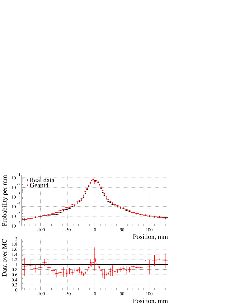
The raw distribution at detector level for a few of the targets are now shown. Figure 13 shows the combined data from the two thin lithium targets. The thickness of this sample corresponds to the second lowest fraction of a radiation length of material used, and it therefore has a narrow distribution. GEANT tends to overestimate the distribution, starting from about 10 mrad. Note that outside about 100 mm the distribution is completely dominated by the scattering from the collimator, see figure 3, and the contribution from the lithium is negligible. Thus the convergence of data and simulation in the tails is more related to the simulation of the collimator than the physics of scattering.

Figure 14: The distribution of particles at detector plane 1 in data and simulation for thin Fe, target 10

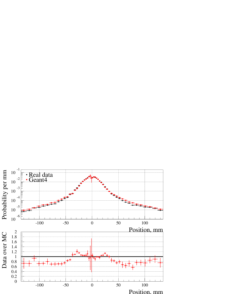
The thin iron target, figure 14, is the highest $Z$ target studied. The GEANT description is better than for any of the lighter targets, but there is here a small region below 40 mm where the scattering distribution is underestimated which is seen in no other target.

Figure 15: The distribution of particles at detector plane 1 in data and simulation for 159 mm of liquid H₂.

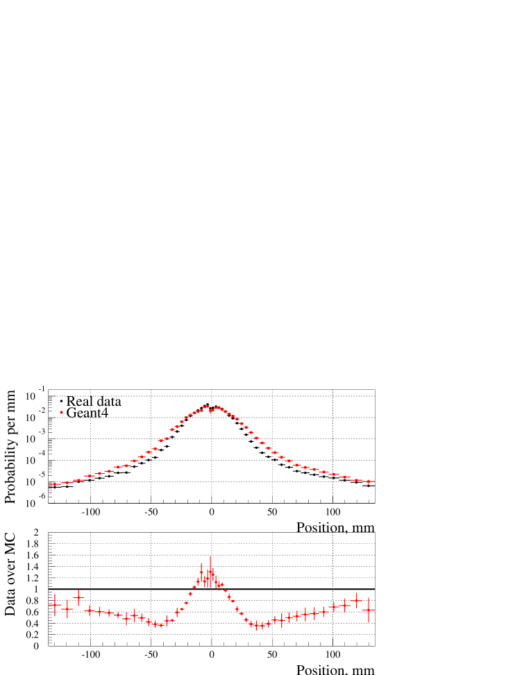
The final comparison presented at the level of the detector is for the longer hydrogen target. This resembles the lithium target, but the differences between data and simulation are more pronounced, with the observed distribution less than half the predicted level at $\pm$40 mm.

8.2 Deconvoluted results

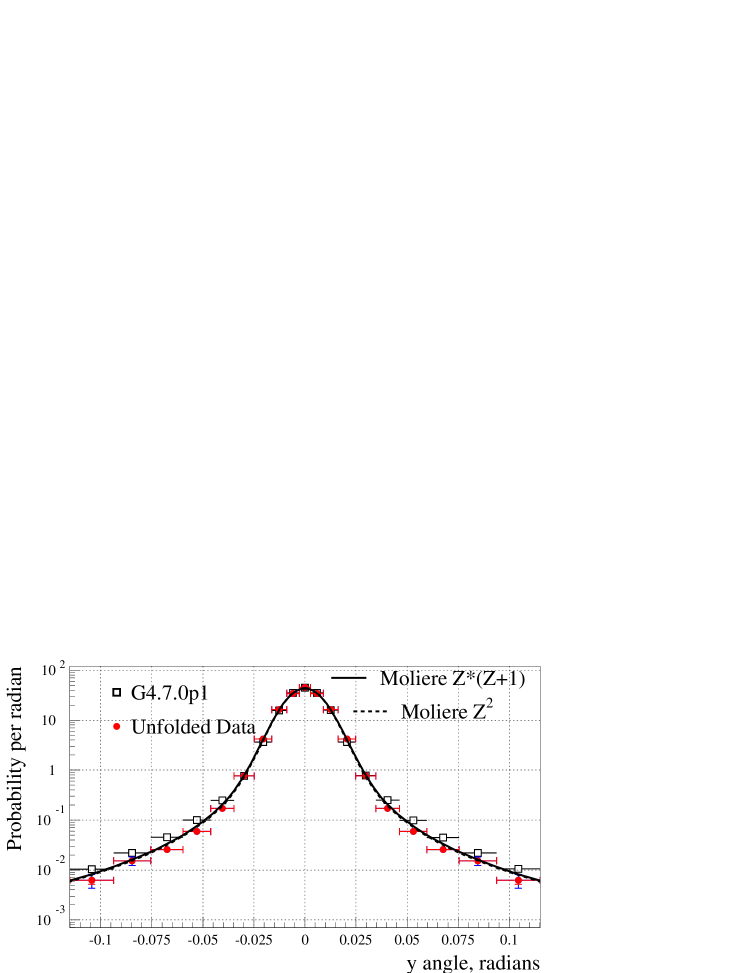
The deconvolution procedure described in section 7 is applied to each of the targets. A series of systematic effects are allowed for, and plots for many of the targets are presented in figures 16 to 22. In each case the statistical error is indicated with an inner error bar, and the combined statistical plus systematic error is indicated with the outer error bar. In most cases the statistical errors are only important for regions of the distribution where the probability of arrival is below about 0.1 per radian. The data for all targets are shown in table 2.

The plots have two smooth curves superimposed: the solid line represents the Moliere calculation with a $Z\times(Z+1)$ factor for the large angle scatters, as proposed by Betheref:bethe , and the dashed line represents the same calculation using a $Z^{2}$ term. The difference corresponds to scattering solely on the nucleus, or also on the electrons. Note that the kinematics of scattering prevent a muon from making a single scatter from a free electron through an angle greater than $m_{e}/m_{\mu}$, or 5 mrad. We therefore expect that for the description of the tail region, above 15 or 20 mrad, the $Z^{2}$ term will be more appropriate.

Figure 16: The projected scattering angle distribution in data and simulation for thin iron, target 10.

• Thin Iron. The data are shown in figure 16. The two Moliere models are almost indistinguishable, and provide a good description of the data. In general, the GEANT 4.7.0p1 simulations are somewhat in excess of the data above 35 mrad. Errors are around 5%, growing to 30% in the final bin shown.

  

  Figure 17: The projected scattering angle distribution in data and simulation for aluminium, target 8.

• Aluminium. The data, figure 17, are rather similar to the iron, with an overestimation of the tail by GEANT 4 of around a factor two.

  

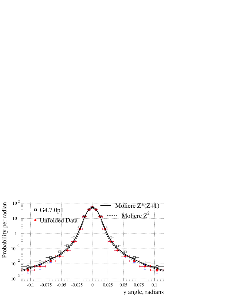
  Figure 18: The projected scattering angle distribution in data and simulation for carbon, target 7.

• Carbon. The data, shown in figure 18, reveal a visually apparent distinction between the Moliere models. Furthermore, the GEANT simulation appears to have an excess compared with data starting at lower angles, around 20 mrad, than it did for iron.

• Polyethylene The data for this target resemble beryllium, with a similar overestimate from GEANT of the scattering. They are not shown. The largest systematic contributions come from the simulated collimator description.

  

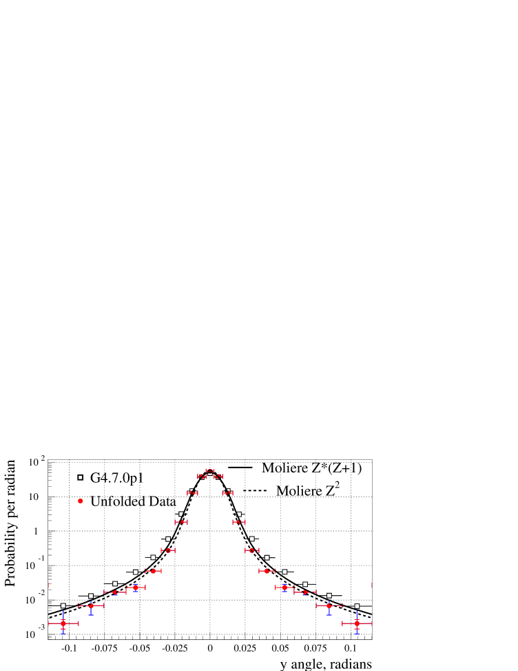
  Figure 19: The projected scattering angle distribution in data and simulation for thick beryllium, target 5.

• Beryllium The thick target data are shown in figure 19. The GEANT model overstates the tails by approximately a factor of two. Of the two Moliere models, the $Z^{2}$ is slightly preferred. No distinction was possible for materials with higher $Z$ as the models were similar. The thin beryllium has larger errors, owing to the large background subtraction required there, and is not displayed.

  

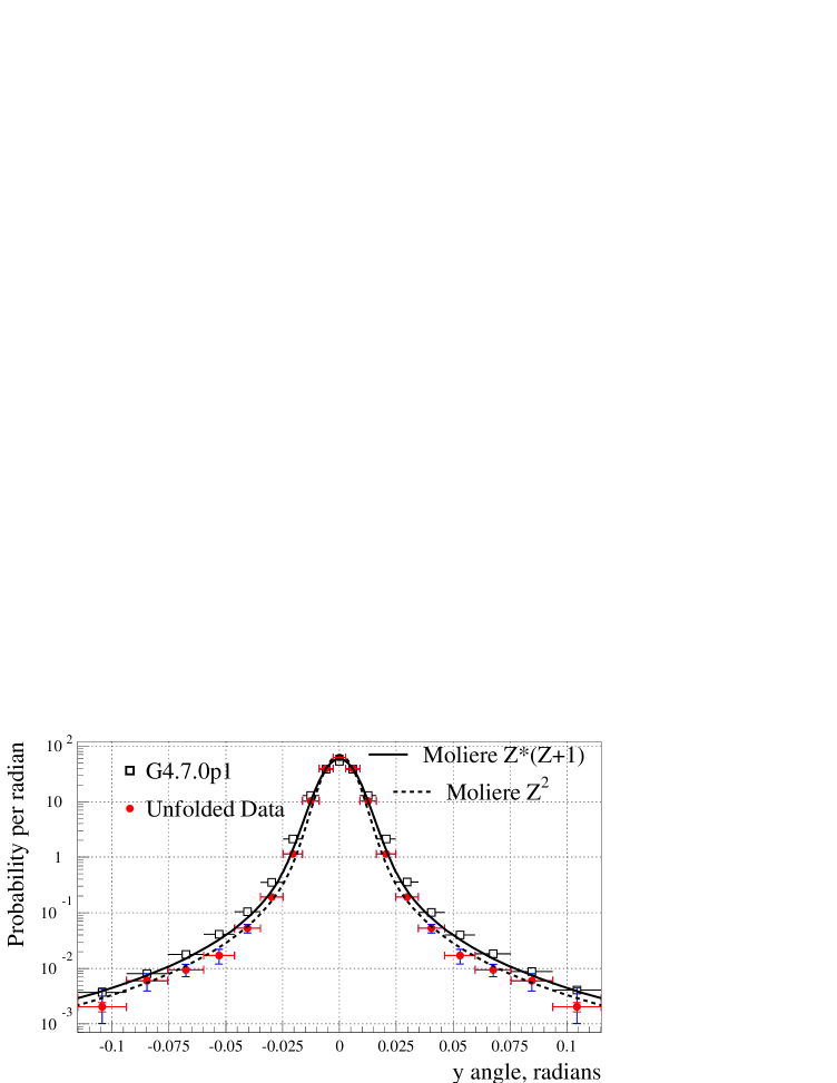
  Figure 20: The projected scattering angle distribution in data and simulation for thick lithium, both targets combined.

• Lithium There were two pairs of lithium targets with very similar thicknesses. The data for the thicker pair are combined in figure 20. The Moliere model with a $Z^{2}$ term provides a reasonable description of the data, but the $Z\times(Z+1)$ Moliere model is now clearly disfavoured. GEANT continues to have tails about a factor two above the data. The data from the thin lithium targets have large systematic and statistical errors in the tails, owing to the large fraction of background which has been accounted for in the deconvolution, and are not shown.

  

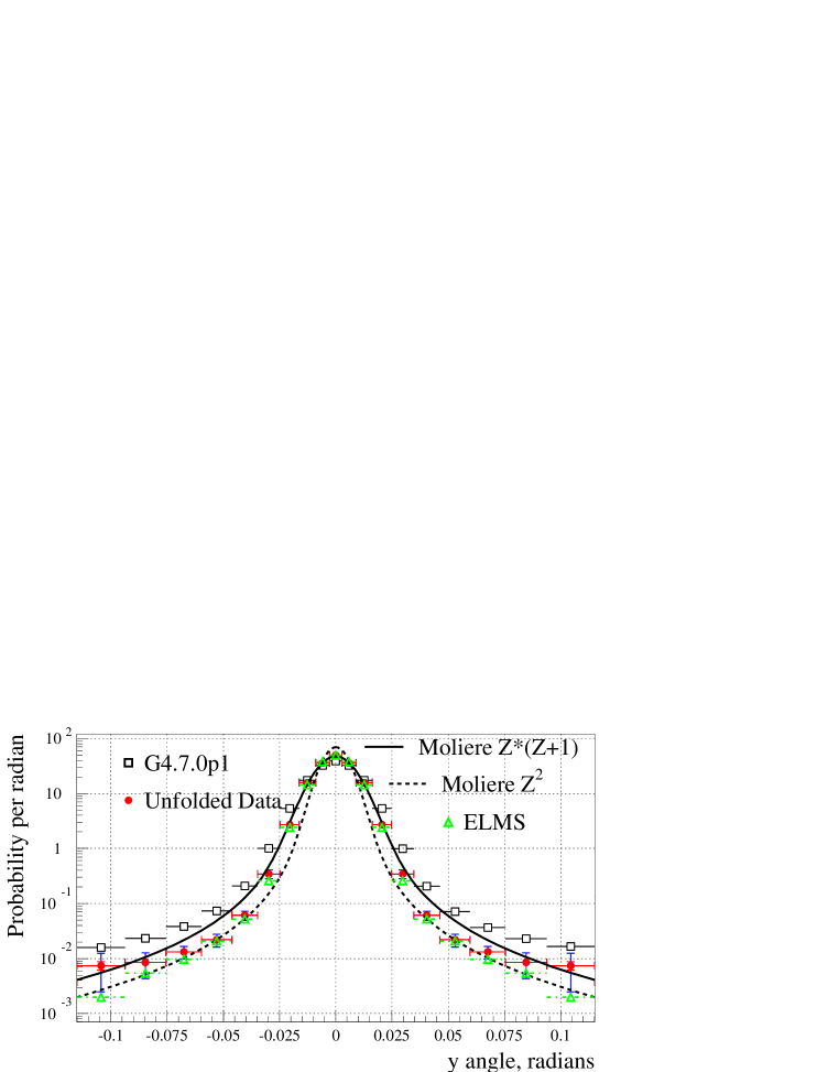
  Figure 21: The projected scattering angle distribution in data and simulation for 109 mm of liquid H₂.

• Hydrogen For 109 mm of hydrogen it can be clearly seen in figure 21 that neither Moliere model accurately describes the data. The $Z^{2}$ model understates the region below around 25 mrad, and above 60 mrad, although here the errors are much larger. GEANT 4.7.0p01 predicts too much scattering, by a factor of around 4 at 50 mrad.

  The data from the ELMS modelref:elms are also compared with our results. These seem to show good agreement at all but the high angle. This region is has the largest systematic errors.

  

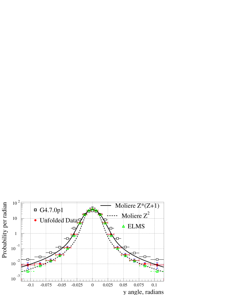
  Figure 22: The projected scattering angle distribution in data and simulation for 159 mm of liquid H₂.

  It can be clearly seen in figure 22 that neither Moliere model accurately describes the data for the long hydrogen target. The $Z^{2}$ model seems correct beyond around 40 mrad, but in the multiple-scattering dominated region the $Z\times(Z+1)$ model is much more appropriate. GEANT 4.7.0p01 predicts too much scattering, but close examination reveals that the excess is less than for the thinner sample.

Overall, we see that when the two Moliere models are distinguishable, i.e. when $Z$ is small, the data is described by the $Z\times(Z+1)$ in the Gaussian core, while the tails show better agreement with the $Z^{2}$ version. This emphasises that the difficulty of describing the data is greater at low $Z$.

GEANT 4.7.0p01 typically predicts about a factor two more scattering tail than is observed. This is not a very large effect given that the data cover 4 orders of magnitude. However, in the case of liquid hydrogen the discrepancy grows to be a factor 4.

The ELMS simulation describes hydrogen very well.

8.3 Systematic Errors

Systematic errors are evaluated by performing the complete analysis with different treatment of the data. The difference with the main results is taken as an estimate of systematic error. All errors are combined in quadrature.

8.3.1 Collimator Description

Three different techniques are used to evaluate the impact of differences between the collimated distributions seen in figure 3. The largest systematic errors are generally from uncertainty in our understanding of the collimated beam.

• Collimator difference The bare collimator distribution seen in simulation is subtracted from the observed data. This residual is then added to the simulated distribution for whichever target is currently under study. This is not completely correct, as it ignores the scattering in the target, but it provides an estimate of the systematic effects.

• Collimator deconvolution The deconvolution to find the underlying scattering distribution is performed on the data with no target present. This would yield a delta function, but does not due to bin width effects and discrepancies between data and simulation. The same is done in simulation, and the difference of the two is found. This difference is due to poor modelling of the collimated beam. The deconvolution for any given target is then repeated with this difference distribution included as an extra convolution term on the right hand side of equation 1. Any changes in the results are taken as systematic errors.

• Internal veto scintillators The collimation system, described in section 2.2, has two internal veto scintillators mounted just before the second collimator. The data show a good separation between pedestal and hits, but there is no complete cross-check on this. The simulated efficiency is lowered to 90%, (which also provides a slightly better description of the scattering distributions) and a systematic error is generated.

8.3.2 Detector alignment

Detector misalignment relative to the simulation will cause errors in the deconvolution.

• Detector X alignment Any credible X misalignment will have negligible impact.

• Detector Y alignment A transverse shift of the detector of 0.1 mm is allowed as a systematic error. The size comes from inspection of figure 3.

• Detector Z alignment The Z position of the detector affects the widths of the distribution. From a combination of studying internal distributions in the tracker and knowledge of the detector construction a systematic error of 5 mm has been assigned.

8.3.3 Detector modelling

• Thick target comparison The muon tracking efficiency maps directly into the scattering distribution, and as such it must be well controlled. The distributions in data and simulation observed with the thick iron target present, figure 7, are used to monitor this. It is conservatively assumed that all differences are due to efficiency, and so the ratio of these distributions is used as an efficiency correction. The change in the unfolded results when this is applied is regarded as a systematic error.

• Cross-talk suppression The default cut selection allows one or two hits to be reconstructed on the first detector plane. When we require exactly one the probability of picking the wrong one is reduced. The analysis is repeated with this requirement and the difference is taken as a systematic error.

8.4 Pion contamination

As discussed in section 6.2, a pion background of 0.8% is estimated. However, this comes from the observation that figure 8 has tails to the left of the muon peak; some of this background will arise from sources other than pions. The most extreme alternative assumption is that there are no pions present, and this is used to estimate a systematic error.

8.5 Deconvolution matrix

The matrix used to relate true scattering angle to measured position is taken from simulation. It depends upon the physics in that simulation, especially scattering in the X direction. This dependence is reduced by re-weighting all the simulated events as a function of the space angle scatter with an ad-hoc simple function which moves GEANT 4 towards Moliere $Z^{2}$ scattering above about 40 mrad. The central values of all the fits have been obtained using this procedure. A systematic error is assigned by comparing with the unweighted GEANT, except in the case of hydrogen where we have the ELMS simulation, and the alternative distribution is GEANT 4 re-weighted to match the predictions of that. This is typically the largest systematic error at the edge of the deconvoluted distributions.

9 Conclusions

These data allow the validation of codes to calculate multiple scattering in the regime relevant for ionisation cooling. In general Moliere scattering provides a good description, but for $Z$ below about 4 there are differences which may be important. In particular, for hydrogen neither Moliere model used is appropriate. The ELMS simulation provides a good prediction of the deconvoluted hydrogen distributions.

The data show noticeable deviations from the predictions of the GEANT 4.7.0p01 simulation code, which tends to overstate the scattering tail by about a factor of two, and more strongly the lower the $Z$ of the material. For hydrogen it is about a factor of 4.

The discrepancies observed previouslyref:andrievsky are not confirmed. Indeed, the scattering predicted by the GEANT simulation needs to be reduced to match the data, not increased.

10 Acknowledgements

We would like to thank all the staff of TRIUMF Laboratory for the helpful and friendly way in which we were welcomed to the laboratory and for all the facilities that were put at our disposal. The following all lent support, for which we are most grateful: M-P.Boudet, R.Barlow, S.Burge, J.Flynn, R.Hampton, D.Laihem, S.Malton, C.Marshall, E.O’Neill, P.Rock, W.Sievers, D.Wade, P.Zubko

We also acknowledge the financial support from PPARC and CCLRC.

11 Appendix

	X0		Upper edge of bin, radians
	%	Type	0.00269	0.00895	0.0162	0.0248	0.0347	0.0463
Li	0.41	data	89.4$\pm$4.4	37.3$\pm$1.7	3.49$\pm$0.27	0.31$\pm$0.05	0.08$\pm$0.02	0.017$\pm$0.009
		G4	75.6$\pm$0.1	39.7$\pm$.04	5.64$\pm$0.01	0.56$\pm$.004	0.13$\pm$.002	0.046$\pm$0.001
	0.82	data	61.7$\pm$3.4	39.3$\pm$1.3	10.3$\pm$0.21	1.14$\pm$0.06	0.19$\pm$0.02	0.053$\pm$0.009
		G4	53.1$\pm$.04	38.3$\pm$.03	12.9$\pm$0.02	2.13$\pm$.007	0.36$\pm$.003	0.101$\pm$0.001
Be	0.28	data	112.$\pm$4.9	29.9$\pm$2.0	1.43$\pm$0.17	0.16$\pm$0.04	0.04$\pm$0.014	0.013$\pm$0.011
		G4	95.1.$\pm$0.1	35.4$\pm$.03	2.55$\pm$0.01	0.33$\pm$.003	0.09$\pm$0.002	0.033$\pm$0.001
	1.06	Data	54.2$\pm$5.4	38.4$\pm$1.2	12.7$\pm$0.63	1.82$\pm$0.17	0.27$\pm$0.025	0.069$\pm$0.010
		G4	48.0$\pm$0.05	36.5$\pm$0.04	14.6$\pm$0.02	3.10$\pm$0.01	0.60$\pm$0.004	0.170$\pm$0.002
CH2	0.99	data	55.4$\pm$3.1	38.2$\pm$1.3	12.6$\pm$0.18	1.79$\pm$0.10	0.28$\pm$0.020	0.073$\pm$0.010
		G4	50.2$\pm$.05	37.2$\pm$.04	13.9$\pm$0.02	2.68$\pm$.009	0.49$\pm$0.004	0.140$\pm$0.002
C	1.53	data	55.7$\pm$3.0	37.8$\pm$1.3	12.7$\pm$0.18	1.97$\pm$0.08	0.29$\pm$0.022	0.076$\pm$0.010
		G4	50.3$\pm$.05	37.2$\pm$.04	13.7$\pm$0.02	2.67$\pm$.009	0.52$\pm$0.004	0.153$\pm$0.002
Al	1.69	data	41.7$\pm$2.4	33.0$\pm$1.0	17.2$\pm$0.20	4.82$\pm$0.10	0.96$\pm$0.040	0.198$\pm$0.014
		G4	39.8$\pm$.04	32.9$\pm$.03	17.0$\pm$0.02	5.14$\pm$0.01	1.15$\pm$0.006	0.327$\pm$0.003
Fe	0.82	data	45.4$\pm$2.8	34.4$\pm$1.1	16.3$\pm$0.15	4.19$\pm$0.10	0.76$\pm$0.034	0.171$\pm$0.012
		G4	44.4$\pm$.05	35.3$\pm$.04	15.8$\pm$0.02	3.64$\pm$0.01	0.78$\pm$0.004	0.250$\pm$0.002
H2	1.31	data	49.5$\pm$2.7	35.8$\pm$1.5	15.7$\pm$0.41	2.70$\pm$0.39	0.34$\pm$0.061	0.061$\pm$0.012
		G4	38.7$\pm$.04	32.2$\pm$.03	17.4$\pm$0.02	5.33$\pm$0.01	1.00$\pm$0.005	0.205$\pm$0.002
		ELMS	49.6$\pm$.07	37.7$\pm$.05	14.5$\pm$0.03	2.43$\pm$0.01	0.26$\pm$0.004	0.052$\pm$0.001
	1.90	data	40.6$\pm$1.7	32.3$\pm$0.9	18.3$\pm$0.18	5.10$\pm$0.38	0.88$\pm$0.014	0.117$\pm$0.028
		G4	31.4$\pm$.04	27.9$\pm$.03	18.3$\pm$.025	8.06$\pm$0.02	2.22$\pm$0.008	0.466$\pm$0.003
		ELMS	40.9$\pm$.06	33.8$\pm$.05	17.5$\pm$0.03	4.86$\pm$0.02	0.72$\pm$0.006	0.103$\pm$0.002
	X0		Upper edge of bin, radians
	%	Type	0.0597	0.0754	0.0938	0.1151	3.141
Li	0.41	data	0.010$\pm$0.006	0.008$\pm$0.004	0.004$\pm$0.003	0.003$\pm$0.002	0.0026$\pm$0.0026
		G4	0.018$\pm$0.001	0.008$\pm$.0004	0.004$\pm$.0002	0.002$\pm$.0001	1.8E-05$\pm$1.8E-06
	0.82	data	0.017$\pm$0.005	0.009$\pm$0.002	0.006$\pm$0.002	0.002$\pm$0.002	0.0007$\pm$0.0007
		G4	0.040$\pm$.0007	0.018$\pm$.0005	0.009$\pm$.0003	0.004$\pm$0.002	3.6E-05$\pm$1.8E-06
Be	0.28	data	0.006$\pm$0.005	0.001$\pm$0.003	0.004$\pm$0.004	0.003$\pm$0.003	0.00017$\pm$0.00017
		G4	0.014$\pm$0.001	0.007$\pm$.0003	0.003$\pm$.0002	0.002$\pm$.0001	1.8E-05$\pm$1.8E-06
	1.06	Data	0.023$\pm$0.006	0.017$\pm$0.003	0.007$\pm$0.003	0.002$\pm$0.0031	0.0024$\pm$0.0024
		G4	0.065$\pm$0.001	0.029$\pm$.0007	0.013$\pm$.0004	0.007$\pm$0.0003	7.2E-05$\pm$0.2E-05
CH2	0.99	data	0.023$\pm$0.005	0.013$\pm$0.002	0.008$\pm$0.003	0.002$\pm$0.002	0.0005$\pm$0.0005
		G4	0.054$\pm$0.001	0.025$\pm$.0006	0.012$\pm$.0004	0.006$\pm$.0003	5.4E-05$\pm$1.8E-06
C	1.53	data	0.032$\pm$0.008	0.015$\pm$0.003	0.007$\pm$0.002	0.004$\pm$0.001	0.0011$\pm$0.0011
		G4	0.061$\pm$0.001	0.026$\pm$.0006	0.013$\pm$.0004	0.007$\pm$.0003	5.4E-05$\pm$1.8E-06
Al	1.69	data	0.071$\pm$0.009	0.028$\pm$0.003	0.018$\pm$0.003	0.005$\pm$0.002	0.0008$\pm$0.0008
		G4	0.124$\pm$0.002	0.055$\pm$0.001	0.026$\pm$.0006	0.013$\pm$.0004	0.00010$\pm$3.6E-06
Fe	0.82	data	0.059$\pm$0.008	0.026$\pm$0.003	0.015$\pm$0.003	0.006$\pm$0.002	0.0014$\pm$0.0013
		G4	0.099$\pm$0.001	0.045$\pm$.0008	0.022$\pm$.0005	0.011$\pm$.0004	9.0E-05$\pm$1.8E-06
H2	1.31	data	0.022$\pm$0.006	0.013$\pm$0.003	0.008$\pm$0.004	0.007$\pm$0.005	0.0025$\pm$0.0025
		G4	0.071$\pm$0.001	0.036$\pm$.0008	0.023$\pm$.0006	0.017$\pm$.0004	0.0024$\pm$1.4E-05
		ELMS	0.021$\pm$.0009	0.010$\pm$.0006	0.005$\pm$.0004	0.002$\pm$.0002	1.8E-05$\pm$1.8E-06
	1.90	data	0.039$\pm$0.009	0.017$\pm$0.004	0.010$\pm$0.002	0.008$\pm$0.003	0.004$\pm$0.004
		G4	0.128$\pm$.0015	0.052$\pm$.0009	0.029$\pm$.0006	0.019$\pm$.0005	0.0025$\pm$1.5E-05
		ELMS	0.034$\pm$0.001	0.016$\pm$.0007	0.007$\pm$.0004	0.003$\pm$.0003	3.6E-05$\pm$0.2E-05

Table 2: The data and simulated predictions for the probability per radian of scattering through a given projected angle. The table is split on two halves to fit the page. The first bin starts at zero. The errors on each bin are total errors. Note that the last bin is essentially an overflow bin and has 100% errors.

References

- (1) D. V. Neuffer, Muon cooling and applications, Proc. Workshop on Beam Cooling, Montreux 1993, CERN Rep. 94-03, 1994, p 49.
- (2) A. I. Andrievsky et al., J. Phys. (USSR) 6 (1942) 279
- (3) V. G. Moliere, Z. Naturforschg 3a (1948) 78; W. T. Scott, Rev. Mod. Phys. 35 (1963) 231
- (4) US Muon Collaboration technical note 123, 1998. http://www-mucool.fnal.gov/notes/notes.html
- (5) S. Agostinelli et al., Nucl. Instrum. Meth. A 506 (2003) 250-303.
-
(6)
W. W. M. Allison, J. Phys G; Nucl. Part. Phys. 29 (2003) 1701-1703.
and http://www-pnp.physics.ox.ac.uk/ holmess/ELMS/ - (7) C. E. Waltham et al., Nucl. Instrum. Meth. A 256 (1987) 91-97
- (8) Hammamatsu photonics R5900U-L16 Multianode 16 Channel Linear Array.
- (9) Minuit CERN Program Library entry D506
- (10) H. Bethe, Phys. Rev. 89, (1953) 1256-1266