Experimental Study of $\chi_{b}$(2P)$\to\pi\pi\chi_{b}$(1P)

Abstract

We have searched for the di-pion transition $\chi_{b}$(2P)$\to\pi\pi\chi_{b}$(1P) in the CLEO III sample of $\Upsilon{\rm(3S)}$ decays in the exclusive decay chain: $\Upsilon{\rm(3S)}\to\gamma\chi_{b}$(2P), $\chi_{b}$(2P)$\to\pi\pi\chi_{b}$(1P), $\chi_{b}$(1P)$\to\gamma\Upsilon$(1S), $\Upsilon$(1S)$\to\ell^{+}\ell^{-}$. Our studies include both $\pi^{+}\pi^{-}$ and $\pi^{0}\pi^{0}$, each analyzed both in fully reconstructed events and in events with one pion undetected. We show that the null hypothesis is not substantiated. Under reasonable assumptions, we find the partial decay width to be $\Gamma(\chi_{b}$(2P)$\to\pi\pi\chi_{b}$(1P)$)=(0.83\pm 0.22\pm 0.08\pm 0.19)~{}{\rm keV},$ with the uncertainties being statistical, internal CLEO systematics, and common systematics from outside sources.

I Introductory Material

Heavy quarkonia, either $c\overline{c}$ or $b\overline{b}$, have provided good laboratories for the study of the strong interaction. New, large data samples at CLEO/CESR and BES/BEPC have renewed the interest in heavy quarkoniaQWG .

Although copiously produced in electric dipole (E1) transitions from the $\Upsilon{\rm(3S)}$ and $\Upsilon$(2S), the $\chi_{b}^{\prime}$ ($2^{3}P_{J^{\prime}}$) and $\chi_{b}$ ($1^{3}P_{J}$) are largely unexplored. The dominant hadronic transitions among the heavy quarkonia involve di-pion emission, characterized by YanYan as the emission of two soft gluons which then hadronize as a di-pion system. These have been studied for transitions among the quarkonia ${}^{3}S_{1}$ states, but have not been observed in other quarkonia transitions such as $\eta_{c}^{\prime}\to\pi\pi\eta_{c}$ or the $\chi_{b}^{\prime}$ decays, which are the subject of this work.

New interest in $\chi_{b}^{\prime}$ decays has also been generated by the CLEO observationomegaPRL of a large branching fraction for the decay $\chi_{b}^{\prime}\to\omega\Upsilon$(1S). This is the only presently known hadronic decay of the $P$-wave $b\bar{b}$ states and the only hadronic bottomonium transition that is not through $\pi\pi$.

We have investigated another hadronic transition of the $\chi_{b}^{\prime}$, namely $\chi_{b}^{\prime}\to\pi\pi\chi_{b}$. As shown in Fig. 1, this search starts with the E1 transition $\Upsilon{\rm(3S)}\to\gamma_{1}\chi_{b}^{\prime}$, followed by the signal process $\chi_{b}^{\prime}\to\pi\pi\chi_{b}$, and the resulting $\chi_{b}$ decay (again via an E1 transition) as $\chi_{b}\to\gamma_{2}\Upsilon$(1S) with $\Upsilon$(1S)$\to\ell^{+}\ell^{-}$. Thus the final state has two photons, two low-momentum (“soft”) pions and two high-momentum leptons. In this Article we (i) establish this $\chi_{b}^{\prime}$ decay and, with reasonable assumptions, (ii) estimate the partial width $\Gamma_{\pi\pi}\equiv\Gamma(\chi_{b}$(2P)$\to\pi\pi\chi_{b}$(1P)$)$.

The main background to our signal, also shown in Fig. 1, has $\Upsilon{\rm(3S)}\to\pi\pi\Upsilon$(2S), followed by an E1 cascade through the $\chi_{b}$ states to the $\Upsilon$(1S). This background process, which we will denote as “$\pi\pi~{}\gamma~{}\gamma$”, has the same number of pions, leptons and photons, with similar kinematics. While this means we need stringent selection criteria to define the signal, it also provides a known process with a nearly identical final state against which to test our analysis procedures.

The data were collected at the Cornell Electron Storage Ring using the CLEO IIIViehhauser detector configuration. The components most critical for this analysis were the Cs-I electromagnetic calorimeter and the charged particle tracking system, each covering $\sim$93% of the $4\pi$ solid angle. Consisting of 7800 crystals, the calorimeter was originally installed in the CLEO II configurationKubota , with some reshaping and restacking for CLEO III to allow more complete solid angle coverage. The shower energy resolution, $\sigma_{E}/E$, is 4% at 100 MeV and 2% at 1 GeV in the barrel region, defined as $|(\cos\theta)|<0.80$, with $\theta$ the dip angle with respect to the beam axis. Complemented at small radius by a 4-layer double-sided silicon vertex detector, a new drift chamberPeterson was installed for CLEO III; its endplate design minimizes material, enhancing the resolution of the endcap electromagnetic calorimeter, extending the solid angle coverage to $|(\cos\theta)|\sim 0.93$.

The signal was searched for in 1.39 fb^-1 of data accumulated at the center of mass energy corresponding to the $\Upsilon{\rm(3S)}$ resonance, consisting of $(5.81\pm 0.12)\cdot 10^{6}$ resonance decays1D . We also used 8.6 fb^-1 of data taken at $\sqrt{s}\approx 10.56$ GeV (“high-energy continuum”) and 0.78 fb^-1 of data taken at the $\Upsilon$(2S), or roughly $5.5\cdot 10^{6}$ decaysArtusoetal , to study and evaluate backgrounds.

We used large Monte Carlo simulations based on GEANT3.211/11GEANT to estimate our efficiencies and tune our selection criteria. In addition to the signal process, we simulated: (i) the main background process, “$\pi\pi~{}\gamma~{}\gamma$”, as described above and in Fig. 1; (ii) $\Upsilon{\rm(3S)}\to\pi\pi\Upsilon$(2S) with $\Upsilon$(2S)$\to\ell^{+}\ell^{-}$, a process with higher statistics and similar pion kinematics, to help confirm our efficiency determinations; (iii) $\Upsilon{\rm(3S)}\to\pi\pi\Upsilon$(2S) with $\Upsilon$(2S)$\to\pi^{0}\pi^{0}\Upsilon$(1S), which could mimic our signal multiplicity if two photons were missed; (iv) “generic” $\Upsilon{\rm(3S)}$ Monte Carlo, which uses all known properties and modes of $\Upsilon{\rm(3S)}$ decay, but for which the backgrounds (i) through (iii) are tagged and not analyzed; (v) $q\overline{q}(q=u,d,s,c)$ continuum processes at the $\Upsilon{\rm(3S)}$ center of mass energy; (vii) for the charged pion decay channel, $\Upsilon{\rm(3S)}\to\gamma\chi_{b}^{\prime}$ with $\chi_{b}^{\prime}\to\omega\Upsilon$(1S) and $\Upsilon$(1S)$\to\ell^{+}\ell^{-}$, which has the same initial photon transition as our signal but would have an additional photon in the decay of the $\pi^{0}$ resulting from the $\omega$ decay to $\pi^{+}\pi^{-}\pi^{0}$; and (viii) for the neutral pion decay channel, $\Upsilon{\rm(3S)}\to\eta\Upsilon$(1S) with $\eta\to\pi^{0}\pi^{0}\pi^{0}$; we used ${\cal B}(\Upsilon{\rm(3S)}\to\eta\Upsilon$(1S)$)=2.2\cdot 10^{-3}$, which is the present 90% CL upper limit for this decay.

In our studies we assumed that there were no $D$-wave contributions to the decays, only $S$-wave, so that $J^{\prime}=J$. This assumption is supported by: (a) the maximum available energy, $Q$, for the nine possible decays is $M(\chi_{b2}^{\prime})-M(\chi_{b0})-2M(\pi^{\pm})$ = 130 MeV, making it difficult to have the extra kinetic energy associated with two units of angular momentum; (b) previous studies of $\Upsilon{\rm(3S)}$$\to\pi\pi\Upsilon$(1S)CLEO3Sto1S94 and $\psi^{\prime}\to\pi\pi J/\psi$BES , systems with substantially more $Q$, indicate no angular momentum between the final state onium and the dipion system, although the former result is also consistentQWG with a few percent of $D$-wave; and (c), the average (weighted by the observed distribution of di-pion invariant mass, $m_{\pi\pi}$) of the $D$-wave between the two pions in $\psi^{\prime}\to\pi\pi J/\psi$BES is less than 10%.

As shown in Table 1, the entry and exit branching fractionsPDG strongly disfavor our observation of $J^{\prime}=J=0$. We also had to discriminate against this possible mode in order to suppress our dominant background source, “$\pi\pi~{}\gamma~{}\gamma$”, in that there is overlap in the energies of the E1 transition photon for the $J^{\prime}=J=0$ signal process and that of the dominant $J=2$ mode of that background. Therefore, we assumed that the transitions with $J^{\prime}=J=1$ or $2$ dominate. To estimate the relative abundance of these two transitions and, later, to calculate the partial width $\Gamma_{\pi\pi}$, we needed the full widths $\Gamma(\chi_{b2}^{\prime})$ and $\Gamma(\chi_{b1}^{\prime})$. We calculated these using the theoretical E1 partial widths for these two statesKR ; EFG and their experimental E1 branching fractionsPDG ; CLEOII ; CUSB to $\gamma\Upsilon$(1S) and $\gamma\Upsilon$(2S), where in the latter we took into account the new CLEO III valueDanko of ${\cal B}(\Upsilon$(2S)$\to\mu^{+}\mu^{-})$. Our results, also listed in Table 1, are $\Gamma(\chi_{b2}^{\prime})=(138\pm 19)$ keV and $\Gamma(\chi_{b1}^{\prime})=(96\pm 16)$ keV. Given ${\cal B}_{\gamma_{1},J^{\prime}}\cdot{\cal B}_{J,\gamma_{2}}/\Gamma$ from this table we expected the $J^{\prime}=J=1$ transition to dominate $J^{\prime}=J=2$ by roughly a factor of 2.3.

$J^{\prime}$	$J$	$\Delta$ M	${\cal B}_{\gamma_{1},J^{\prime}}$	${\cal B}_{J,\gamma_{2}}$	$\Gamma$	${\cal B}_{\gamma_{1},J^{\prime}}\cdot{\cal B}_{J,\gamma_{2}}/\Gamma$
(2$P$)	(1$P$)	(MeV)	(%)	(%)	(keV)	($\times 10^{-4}$ keV-1)
2	2	356	11.4	22	138	1.8
1	1	363	11.3	35	96	4.1
0	0	372	5.4	$<6$	–	–

Table 1: The three di-pion transitions between $\chi_{b}^{\prime}$ and $\chi_{b}$ that leave the orbital angular momentum unchanged ($S$-wave). The third column is the mass difference. Columns four and five are the branching fractions for the entrance and exit E1 transitions: ${\cal B}_{\gamma_{1},J^{\prime}}={\cal B}(\Upsilon$(3S)$\to\gamma_{1}\chi_{b}^{\prime})$ and ${\cal B}_{J,\gamma_{2}}={\cal B}(\chi_{b}\to\gamma_{2}\Upsilon$(1S)). The E1 transition from $\chi_{b0}$ is unobserved, with a limit of 6% on its branching fraction at 90% C.L..

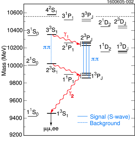
Figure 1: The decay process under study and the main background process, denoted in the text as “$\pi\pi~{}\gamma~{}\gamma$”. Note that these have the same $\gamma_{2}$, so that the energy of this photon is not a distinguishing observable.

Two approaches were taken to evaluate $\chi_{b}^{\prime}\to\pi\pi\chi_{b}$. In the first, the “two-pion” analysis, we required all the particles to be found but made minimal requirements on $\gamma_{2}$. A two-dimensional analysis was performed using the energy of the photon in $\Upsilon$(3S)$\to\gamma_{1}\chi_{b}{\rm(2P)}$, denoted $E_{1}$, and the mass recoiling against the pion pair, $M_{\mathrm{rec}}$, to define our signal. In calculating $M_{\mathrm{rec}}$ we also used the four vector of $\gamma_{1}$ so that $M_{\mathrm{rec}}$ actually represents the mass difference of the $2P$ and $1P$ states; i.e.,

$$M_{\mathrm{rec}}\equiv\sqrt{({\cal P}_{3S}-{\cal P}_{\gamma 1})^{2}}-\sqrt{({\cal P}_{3S}-{\cal P}_{\gamma 1}-{\cal P}_{\pi 1}-{\cal P}_{\pi 2})^{2}}~{},$$ (1)

with ${\cal P}$ denoting the four-vector momentum. In the second, we increased our efficiency by only reconstructing one of the pions (a “one-pion” analysis) and used as variables the missing mass of the event and $E_{1}$.

II The Channel $\chi_{b}^{\prime}\to\pi^{+}\pi^{-}\chi_{b}$

In event selection for our study of $\chi_{b}^{\prime}\to\pi^{+}\pi^{-}\chi_{b}$ we required four well-measured primary charged tracks, two of which had to have high momenta (in excess of 3.75 GeV/c) and had to have calorimeter and momentum information consistent with being either $e^{+}e^{-}$ or $\mu^{+}\mu^{-}$. These two putative lepton tracks also had to have an invariant mass within 300 MeV of the $\Upsilon$(1S) mass, which is a very loose requirement ($\sim\pm 5\sigma$). The other track(s) had to have measured momentum 50 $<p<$ 750 MeV/c and have a dip angle with respect to the beam axis corresponding to $|\cos\theta|<0.93$. To reduce QED backgrounds and facilitate comparison to other, established channels, we made additional, highly efficient requirements on the difference of the momenta of the two lepton candidates and on the maximum allowed momentum of the charged pion candidates(s).

Transition photon candidates in our analyses of $\chi_{b}^{\prime}\to\pi^{+}\pi^{-}\chi_{b}$ were defined as calorimeter energy depositions, in excess of 60 MeV, with lateral profile consistent with that of a photon, not associated with any charged track or any known “noisy” crystals, and not located in the inner-most portion of the endcap, roughly bounded by $|\cos\theta|\approx 0.93$. For the $e^{+}e^{-}$ channel, we further suppressed fragments of the electron showers.

In the charged two-pion (fully-reconstructed) analysis, we required that there be either two or three photon candidates. If there were two, the higher of the two energies had to be in excess of 300 MeV; otherwise $E_{1}$ was deemed likely to be due to a spurious calorimeter energy deposition. If three were found, then the highest energy had to exceed 300 MeV and the second highest exceed 120 MeV, so that it not be confused with a valid $E_{1}$ photon. Then, based on Monte Carlo studies of $S^{2}/B$, we defined the three regions shown in Fig. 2: a signal region, a region in which we expect the “$\pi\pi~{}\gamma~{}\gamma$” process to dominate, and a larger “sideband” region. The figure also shows how the Monte Carlo simulations of signal (left plot) and “$\pi\pi~{}\gamma~{}\gamma$” (center plot) populate these three regions. The overall efficiency for the signal is 5.1% and 4.3%, for $J^{\prime}=J=1$ and $J^{\prime}=J=2$, respectively, with the largest inefficiency coming from reconstructing two high-quality low-momentum tracks. As described in Sect. IV.2, these have relative uncertainties of $\sim$10%. The efficiencies for the $\mu^{+}\mu^{-}$ final state are 10% (relative) higher than those for the $e^{+}e^{-}$ state in this analysis; this trend is true for the other three analyses in this Article as well.

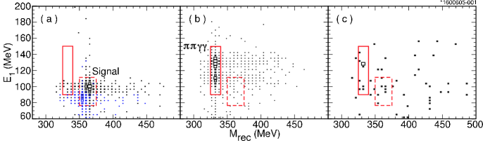
Figure 2: Definition of the three regions in the charged two-pion analysis in the $E_{1}~{}vs.~{}M_{\mathrm{rec}}$ plane. The outline of the figure defines the “sideband” region, which does not include the two smaller regions, namely the solid rectangle in which the $\pi\pi~{}\gamma~{}\gamma$ process dominates and the dashed rectangle in which the signal dominates. On the left (a) we show Monte Carlo events from both the $1\to 1$ and $2\to 2$ transitions, with the production ratio of 2.3:1, as described in the text. In the middle (b) we similarly show Monte Carlo events from the $\pi\pi~{}\gamma~{}\gamma$ process. The data for this two-pion analysis is shown on the right in (c).

Region of	Estimated	Constrained	Number	Estimated	Constrained	Number
Plot	Occupancy	Occupancy	Observed	Occupancy	Occupancy	Observed
	$\pi^{+}\pi^{-}$ found			$\pi^{0}\pi^{0}$ found
Sideband	$22.7\pm 4.4$	$36$	36	$16.5\pm 2.4$	$15$	15
$\pi\pi~{}\gamma~{}\gamma$	$8.6\pm 2.0$	$9.0\pm 2.0$	10	$13.7\pm 3.2$	$13.6\pm 3.2$	15
Signal	$0.6\pm 0.2$	$1.0\pm 0.3$	7	$2.3\pm 0.5$	$2.2\pm 0.5$	1
	One $\pi^{\pm}$ found			One $\pi^{0}$ found
Sideband	$5.2\pm 1.4$	$8$	8	$15.2\pm 3.4$	$17$	17
$\pi\pi~{}\gamma~{}\gamma$	$17.1\pm 4.8$	$18.0\pm 4.9$	26	$14.4\pm 3.2$	$14.8\pm 3.4$	13
Signal	$2.2\pm 0.6$	$2.6\pm 0.7$	17	$26.5\pm 5.7$	$26.9\pm 5.8$	35

Table 2: The results of the four analyses, showing the predicted occupancies in each of the three regions of interest and the observed number of events in those regions. In the “constrained” column the predictions have been adjusted to make that of the sideband region match the observed number in that region.

We also show in the same figure the data for this two-pion analysis, which has 36/10/7 events in the sideband/$\pi\pi~{}\gamma~{}\gamma$/signal regions, respectively.

Using Monte Carlo simulations of the $\Upsilon{\rm(3S)}$ decays and the high-energy continuum data, all properly scaled, we predict the number of expected events in the three regions, as shown in Table 2; the uncertainties listed are from the various branching fractionsPDG used in the scaling to our accumulated number of $\Upsilon{\rm(3S)}$ decays. The prediction for the “$\pi\pi~{}\gamma~{}\gamma$” region (the second line of the table) is very consistent with the observation in data, which also has roughly equal numbers of $e^{+}e^{-}$ (4) and $\mu^{+}\mu^{-}$ (6) final states. The large sideband region prediction is somewhat smaller than the data, particularly in the $e^{+}e^{-}$ final state. To take a more conservative approach to the number of events expected in the signal region due to known processes and backgrounds, we then added in enough events, scaled in proportion to the size of each box, to bring the sideband region into exact balance. This procedure is labeled “constrained occupancy” in Table 2; it predicts $1.0\pm 0.3$ events in the signal region, in which we observe seven, of which six are $\mu^{+}\mu^{-}$.

In addition to observing that the $\pi\pi~{}\gamma~{}\gamma$ region is properly populated ($8.6\pm 2.0$ events expected vs. 10 observed), we checked that our analysis procedures, when instead requiring 0 or 1 photon, can reproduce the measured product branching fraction ${\cal B}(\Upsilon{\rm(3S)}\to\pi^{+}\pi^{-}\Upsilon$(2S)$)$ $\cdot$ ${\cal B}(\Upsilon$(2S)$\to\ell^{+}\ell^{-})$, which is, by weighted average of the results of CLEO IBrock , CLEO IICLEO3Sto1S94 and CUSBWu , $(1.10\pm 0.12)\cdot 10^{-3}$. We observed $154\pm 13$ $\mu^{+}\mu^{-}$ such events and $152\pm 39$ $e^{+}e^{-}$, which implies an efficiency in the CLEO III data of $(4.8\pm 0.8)$%. Our Monte Carlo simulations of this channel indicate an efficiency of $(4.3\pm 0.1)$%, in agreement with the data.

Given the low efficiency for finding low momentum pions, our second approach (the charged one-pion analysis) was to require only one soft charged track but make tighter demands on $\gamma_{2}$ (see Fig. 1) and on the lepton pair. The sum of the measured $E_{1}$ and $E_{2}$ was fit to 518 MeV, the properly weighted average for that sum from our Monte Carlo simulation of the signal, yielding a $\chi^{2}_{\gamma\gamma}$ for the fit as a figure of merit. We required $\chi^{2}_{\gamma\gamma}<4$. The momenta of the lepton pair were used in a mass-constrained fit to the $\Upsilon$(1S) mass, for which we required $\chi^{2}<10$. In constructing the missing mass of the event, which for signal would be $M(\pi)$, we used as inputs the $\Upsilon{\rm(3S)}$ mass, the angles and fitted energies of the two photons, ${\cal P}_{\Upsilon}$ (the momentum four vector of the fitted $\Upsilon$(1S)), and the momentum of the one measured charged pion:

$$M_{\mathrm{miss}}\equiv\sqrt{({\cal P}_{3S}-{\cal P}^{\mathrm{fit}}_{\gamma 1}-{\cal P}^{\mathrm{fit}}_{\gamma 2}-{\cal P}_{\Upsilon}-{\cal P}_{\pi})^{2}}~{}.$$ (2)

Figure 3: Definition of the three regions in the charged one-pion analysis in the $E_{1}~{}vs.~{}M_{\mathrm{miss}}$ plane. In both cases the outline of the figure is the large “sideband” region. On the top (a) we show the smaller “signal” region and the “$\pi\pi~{}\gamma~{}\gamma$” region, and the Monte Carlo events from both the $1\to 1$ and $2\to 2$ transitions. On the bottom (b) we similarly show both of these regions and the Monte Carlo events from the “$\pi\pi~{}\gamma~{}\gamma$” process.

Given that we only observed one of the pions, the calculated di-pion invariant mass for the charged one-pion analysis, namely,

$$m^{2}_{\pi(\pi)}=({\cal P}_{\pi}+{\cal P}_{\mathrm{miss}})^{2}=({\cal P}_{3S}-{\cal P}_{\Upsilon}-{\cal P}^{\mathrm{fit}}_{\gamma 1}-{\cal P}^{\mathrm{fit}}_{\gamma 2})^{2}~{},$$ (3)

was not constrained to be in excess of twice the pion mass. Simulations show a selection criterion of $m_{\pi(\pi)}>260$ MeV to be highly efficient for $\chi_{b}^{\prime}\to\pi^{+}\pi^{-}\chi_{b}$, and this was applied to minimize backgrounds.

We again used a study of $S^{2}/B$ to determine a signal region, this time in the $E_{1}~{}vs.~{}M_{\mathrm{miss}}$ plane, as depicted in Fig. 3. The region assigned to the main background, “$\pi\pi~{}\gamma~{}\gamma$”, was somewhat larger and contiguous to the signal region; the boundaries were selected to have the sideband region have as few events as possible that were either signal or this main background. We found from our Monte Carlo simulations that the overall efficiency for this one-pion analysis is 10.6% for $J^{\prime}=J=1$ and 9.6% for $J^{\prime}=J=2$. As detailed in Sect. IV.2 the (relative) uncertainties in these efficiencies are roughly 10% and 8%, respectively.

The data are shown in Fig. 4 and the yields are listed in Table 2. Of the 17 signal events, nine have $\ell=\mu$ and the other eight have $\ell=e$. The population of the “$\pi\pi~{}\gamma\gamma$” region is consistent with, although a bit larger than, our prediction.

The sideband region also has a somewhat larger yield than predicted, so, as in the two-pion analysis we added in enough background events to balance the sideband region, as shown in the “constrained” column of Table 2. The probability that the backgrounds, constrained to give the sideband yield, could produce the observed population in the signal region is $1.3\cdot 10^{-7}$.

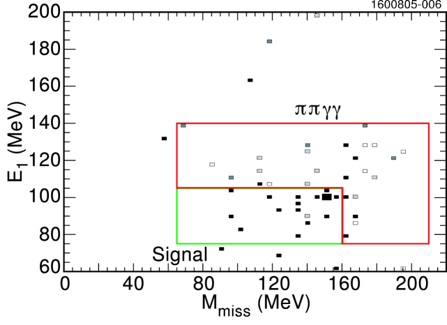
Figure 4: The data events falling into our three defined regions for the charged one-pion analysis, shaded according to their $\chi^{2}_{\gamma\gamma}$ value. The darkest boxes are for events with $\chi^{2}_{\gamma\gamma}$ values between 0 and 1 and the lightest for those with $\chi^{2}_{\gamma\gamma}$ values between 3 and 4. Most of the events in the small signal region (the smaller rectangle) show low values for $\chi^{2}_{\gamma\gamma}$, indicating excellent fits of the photon energy sum to that expected for signal events.

The distribution of $\chi^{2}_{\gamma\gamma}$ for the 17 events in the signal region closely mimics that seen in our Monte Carlo simulation. The values of $\chi^{2}_{\gamma\gamma}$ are encoded in Fig. 4, showing a predominance of low (i.e., better) values of this figure of merit for the events in the signal region. To further test this aspect of the analysis we instead optimized our selection criteria and our constraints for the “$\pi\pi~{}\gamma~{}\gamma$” process. We found 49 events, which imply an efficiency in data of $(15.0\pm 4.8)\%$; our Monte Carlo simulations predicted an efficiency for this test of $(12.7\pm 0.2)\%$, showing consistency.

We also checked that there is not some other, resonance-induced effect that could mimic our charged one-pion signal by analyzing $\Upsilon$(2S) data, with selection criteria and plotted variables appropriately scaled to account for the mass difference between the $\Upsilon$(2S) and the $\Upsilon{\rm(3S)}$ resonances. Only three events passed our selection criteria with none of them in the signal region; we assumed no such background sources in further analysis.

III The Channel $\chi_{b}^{\prime}\to\pi^{0}\pi^{0}\chi_{b}$

Most of the selection criteria for our study involving neutral pions were the same as those in the preceding section. Given the relatively small $Q$ of our process, the photons from the transition $\pi^{0}$ decays tend to be of low energy. Therefore, we lowered the energy cut-off in the calorimeter barrel ($|\cos\theta|<0.80$) to 30 MeV. In the endcap regions ($0.80<|\cos\theta|<0.93$) photons were still required to have energy in excess of 60 MeV. In addition to these photon candidates, we also allowed one endcap shower in the energy range $30<E<60$ MeV to be used as a decay product of the neutral pions. All $\pi^{0}$ candidates were formed from high quality showers that were not associated with charged tracks, with the exception that no $\pi^{0}$ candidate could use the highest energy photon in the event, which was presumed to be from the transition $\chi_{b}\to\gamma\Upsilon$(1S).

For the fully reconstructed, neutral two-pion analysis, there had to be five or more photon candidates and no charged tracks other than the two lepton candidates. We require two or more found $\pi^{0}$ candidates, of which we kept the best two based on their goodness of fit to the $\pi^{0}$ mass hypothesis ($S_{\pi^{0}}\equiv(M_{\gamma\gamma}-M_{\pi^{0}})/\sigma$). We further ensured good $\pi^{0}$ candidates by requiring that the sum of the squares of the two pulls (i.e., the two $\chi^{2}$ values from the $\pi^{0}$ fits) be less than 25. All photon candidates not used in forming the two neutral pions were then investigated in pairs in a fit to 518 MeV, the expected sum of the transition energies $E_{1}$ and $E_{2}$. The best pair was kept; the chi-square of the fit was restricted to $\chi^{2}_{\gamma\gamma}<9$.

Our simulations indicate that the three regions used in the charged two-pion analysis were also optimal for the neutral case, with distributions of the signal and primary background similar to those in Fig. 2. We found the efficiency for a $\pi^{0}\pi^{0}$ signal with $J^{\prime}=J=1$ is 7.2% and for $J^{\prime}=J=2$ is 6.4%, with roughly 11% (relative) uncertainties.

Again using the known branching fractionsPDG , we can predict the occupancies of these three regions in the absence of a signal, as shown in the $\pi^{0}\pi^{0}$ section of Table 2. While the sideband and “$\pi\pi~{}\gamma~{}\gamma$” regions have the expected populations, there is only one event in the signal region. This analysis supports the null hypothesis, with roughly a 90% probability that the predicted occupancy of 2.3 events would give one or more events in that region.

For the neutral one-pion analysis the fit of the $\pi^{0}$ candidate had to be in the range $-7<S_{\pi^{0}}<7$. Because in a typical event there are several photons of energy near 100 MeV and because we required exactly one found $\pi^{0}$, a large combinatoric “$\pi\pi~{}\gamma~{}\gamma$” background can contaminate the signal region.

The highest energy photon in the event was required to have $E>370$ MeV. It was then paired with all other photon candidates not used in forming the lone $\pi^{0}$ to find the best match to the photon energy sum of 518 MeV; for this neutral analysis we require $\chi^{2}_{\gamma\gamma}<3$ (the limit was 4 in the corresponding charged analysis).

Requirements on the reconstructed pion and on the lepton candidates were similar to those of the charged one-pion analysis. In addition we required that the energy of the missing $\pi^{0}$, based on the energies of the found particles, be in the range $100<E_{\mathrm{miss}}<240$ MeV.

The regions for the signal and primary backgrounds from the charged one-pion analysis were not found to be optimal in the neutral case. While the sideband region remained the same, $S^{2}/B$ studies showed the optimal signal region to have $75<E_{1}<110$ MeV and $65<M_{\mathrm{miss}}<210$ MeV and the “$\pi\pi~{}\gamma~{}\gamma$” region to best be $110<E_{1}<140$ MeV and, again, $65<M_{\mathrm{miss}}<210$ MeV. For these selection criteria the efficiencies are 13.4% for $J^{\prime}=J=1$ and 12.3% for $J^{\prime}=J=2$; the relative uncertainties are roughly 16% and 12%, respectively.

The results from the data are shown in Table 2. We find the occupancies of the two non-signal regions again to be near our expectations. For the signal region there is a slight excess, with 35 events being observed but only $26.9\pm 5.8$ expected.

IV Discussion of Results and Summary

IV.1 The Null Hypothesis

We now have four analyses on which to base our test of the null hypothesis that the backgrounds alone can account for the observed data in the signal regions.

In all cases we use the predicted occupancies (which represents the null hypothesis) from the “constrained” column of Table 2, thus allowing for the fact that there may be some background contribution unaccounted for by our simulations and continuum data samples. From this table we generate a large number of experimental mean occupancies and use Poisson statistics to assess the statistical consistency of backgrounds alone with the number of observed events in data (or more).

Charged two-pion analysis: For example, here we create many experiments that have a Gaussian-distributed background level with mean of 1.0 events and standard deviation of 0.3 events. The Poisson probability for this to result in 7 or more observed events is $2.2\cdot 10^{-4}$, or a one-sided Gaussian effect at 3.5$\sigma$.

Charged one-pion analysis: The probability for $2.6\pm 0.7$ events to yield 17 or more is $1.3\cdot 10^{-7}$, or a one-sided Gaussian effect at 5.2$\sigma$.

Neutral two-pion analysis: Similarly, $2.2\pm 0.5$ events have a 87% probability of accounting for the lone signal event, thus supporting the null hypothesis.

Neutral one-pion analysis: The null hypothesis has an 8% probability of accounting for the yield in this analysis.

One can combine the charged and neutral two-pion analyses into one test: they are statistically independent and have the same signal region contour. Summing the entries in Table 2, the probability for $3.3\pm 0.6$ events to yield 8 or more is $2.6\%$.

The analyses with charged pions show a pronounced signal that is supported by the neutral one-pion analysis. Given our predicted backgrounds and the partial width inferred from the charged pion analyses, there is a 2% probability of only seeing zero or one event in the neutral two-pion study. Taking all four analyses together, we conclude that the null hypothesis is not substantiated.

IV.2 Partial Width for the Di-pion Decay

Uncertainty	Charged			Neutral
Source	$\Delta\epsilon/\epsilon$ (%)	$\Delta\epsilon_{1\to 1}$	$\Delta\epsilon_{2\to 2}$	$\Delta\epsilon/\epsilon$ (%)	$\Delta\epsilon_{1\to 1}$	$\Delta\epsilon_{2\to 2}$
Limited MC statistics	-	0.3	0.3	-	0.3	0.3
Running period dependence	-	0.5	small	-	small	small
Signal region definition	-	0.6	0.1	-	1.7	1.0
Shape of $m_{\pi\pi}$ distribution	2	-	-	1	-	-
Decay angular distribution	2	-	-	2	-	-
$\pi^{0}$, $\pi^{\pm}$ and $\ell$ finding	6	-	-	8	-	-
Photon-finding probability	2	-	-	2	-	-
$\ell=e/\mu$ selection	1	-	-	1	-	-
Other selection criteria	-	small	small	-	small	small
Sum	7%	0.8	0.3	10%	1.7	1.0

Table 3: The systematic uncertainties in the efficiencies for the two one-pion analyses. For the correlated efficiencies these are listed as a relative percentage; for the individual uncorrelated effects, absolute values are shown.

Assuming that our data constitute observation of the signal process, we then proceed to obtain values for the partial width for this di-pion transition. We assume there are no $D$-wave contributions and that our observation of the $J^{\prime}=J=0$ transition is suppressed (see Table 1 and the associated discussion). Here we useKY1981 $\Gamma_{\pi\pi}\equiv\Gamma(\chi_{b1}^{\prime}\to\pi\pi\chi_{b1})=\Gamma(\chi_{b2}^{\prime}\to\pi\pi\chi_{b2})$. Invoking isospin as a good quantum number in such strong interaction decays, and neglecting the small effects of the $\pi^{\pm}-\pi^{0}$ mass difference, we also have $\Gamma_{\pi\pi}=\frac{3}{2}\cdot\Gamma_{\pi^{+}\pi^{-}}=3\cdot\Gamma_{\pi^{0}\pi^{0}}$. We then write:

$$N_{\mathrm{sig}}=N_{\Upsilon(3S)}\cdot{\cal B}_{\Upsilon\to\ell^{+}\ell^{-}}\cdot\frac{C}{3}\Gamma_{\pi\pi}\cdot\left[\frac{{\cal B}_{\gamma 1,1}~{}\epsilon_{1\to 1}~{}{\cal B}_{1,\gamma 2}}{\Gamma(\chi_{b1}^{\prime})}+\frac{{\cal B}_{\gamma 1,2}~{}\epsilon_{2\to 2}~{}{\cal B}_{2,\gamma 2}}{\Gamma(\chi_{b2}^{\prime})}\right],$$ (4)

with $C=1$ or 2 in the neutral and charged cases, respectively. Here, $N_{\mathrm{sig}}=N_{\mathrm{obs}}-N_{\mathrm{bck}}$; the second term is the weighted average of the two background estimation schemes in Table 2, and the difference of this average from either scheme is included in the systematic uncertainty. The only statistical uncertainty is in the number of observed events, $\sqrt{N_{\mathrm{obs}}}$. We use ${\cal B}_{\Upsilon\to\ell^{+}\ell^{-}}=(4.96\pm 0.12)\%$, and the four E1 transition branching fractions are as in Ref.PDG and Table 1. The uncertainties in these ${\cal B}$ values, in the values of $\Gamma$ as given earlier, and in the number of parent $\Upsilon{\rm(3S)}$ are taken as systematic in nature. These are effectively “common” to all four analyses at the level of 20-24%, depending slightly on the relative ratios of the two efficiencies in Eqn. 4. The uncertainties in the level of background to be subtracted and in the two efficiencies are “particular” to each of the analyses.

The contributions to the systematic uncertainties to the efficiencies in the two one-pion analyses are shown in Table 3, with those for the two-pion analyses being similar in source and magnitude. As evident from Fig. 3, the selection criterion on $E_{1}$ is very tight for the $J^{\prime}=J=1$ transition in the charged one-pion case, leading to significant uncertainty in the modeling of that process; this is similarly problematic for the neutral one-pion analysis. For the $J^{\prime}=J=2$ transition, the photons from the unfound $\pi^{0}$ in the neutral one-pion analysis lead to a sizeable uncertainty in our modeling near the lower boundary of the signal box.

We have varied the di-pion invariant mass distribution in the Monte Carlo simulations to include three-body phase space, a Yan distributionYan and a flat distribution, and found relative efficiency variations of from 1% (for the charged case) to 2% (for the neutral case). We have included in our stated efficiencies the effect of the angular distribution of the transition photon in $\Upsilon{\rm(3S)}\to\gamma\chi_{b}^{\prime}$ not being isotropic; this is roughly a 2% effect. We have not included such effects for the decay $\chi_{b}\to\gamma\Upsilon$(1S), and posit a 2% uncertainty for this source. For our ability to model the detection of the transition photons we assign an additional systematic uncertainty of 1% per photon.

We take a 1% per track systematic uncertainty for finding the high momentum leptonsLi . For the softer pion tracks we take a 2% per pion uncertainty; this is substantiated by CLEO studies of charged di-pion transitions in the charmonium system and our own checks of the overall efficiency presented in Sect.II. Neutral pion finding efficiencies are checked in CLEO studies of neutral di-pion transitions in the $\Upsilon$ and charmonium systems, for which we assign 3% per pion as the systematic uncertainty for finding (or not finding) a $\pi^{0}$. These particle finding uncertainties are conservatively added linearly in the Table.

There is a small uncertainty in our ability to model the lepton identification requirementsLi , which we conservatively take as 1%. The other entries are found to be negligible, given the generally loose nature of the selection criteria.

To determine the resultant systematic uncertainty for $\Gamma_{\pi\pi}$ we use a toy Monte Carlo, generating all the inputs in Eqn. 4 distributed as Gaussians with their uncertainties, and ask for the region that symmetrically bounds $68.3\%$ of the values.

As discussed in Sect. IV.1, we evaluated $\Gamma_{\pi\pi}$ for three situations: charged one-pion, neutral one-pion, and combined two-pion.

Channel	$N_{\mathrm{obs}}$	$N_{\mathrm{bck}}$	$\epsilon_{1\to 1}$ (%)	$\epsilon_{2\to 2}$ (%)	$\Gamma_{\pi\pi}$ (keV)
Charged one-pion	17	$2.4\pm 0.7$	$(1\pm 0.07)(10.6\pm 0.8)$	$(1\pm 0.07)(9.6\pm 0.3)$	$1.24\pm 0.35\pm 0.12$
Neutral one-pion	35	$26.7\pm 5.8$	$(1\pm 0.10)(13.4\pm 1.7)$	$(1\pm 0.10)(12.3\pm 1.0)$	$1.12\pm 0.80~{}^{+0.82}_{-0.78}$
Charged two-pion	–	–	$(1\pm 0.10)\cdot 5.1$	$(1\pm 0.10)\cdot 4.3$
Neutral two-pion	–	–	$(1\pm 0.11)\cdot 7.2$	$(1\pm 0.11)\cdot 6.4$
Combined two-pion	8	$3.1\pm 0.6$	–	–	$0.52\pm 0.30\pm 0.08$

Table 4: The various contributions to the calculation of the partial width from sources in this experiment. The two two-pion analyses have been combined for the width determination. Of the two quoted uncertainties, the first is statistical and the second is from the uncertainties in $N_{\mathrm{bck}}$ and the efficiencies. An additional systematic uncertainty of $\sim 22\%$ comes from branching fractions, estimates of the total widths, and the number of $\Upsilon{\rm(3S)}$.

The individual contributions to Eqn. 4 are shown in Table 4, along with the value of $\Gamma_{\pi\pi}$ obtained, its statistical uncertainty, and its individual (CLEO-based) systematic uncertainty. Taking the statistical average of the three gives $\Gamma_{\pi\pi}{\rm[stat~{}only]}=(0.84\pm 0.22)$ keV. A more complete average takes into account the individual systematic uncertainties; this weighted average is $\Gamma_{\pi\pi}=(0.83\pm 0.23)$ keV. Following the PDGPDG prescription for evaluating the consistency of results being averaged, we obtain an uncertainty scale factor of 1.09, which is close to unity.

De-convolving the statistical uncertainty and adding in a separate term for the 22% “common” uncertainties that are not based on measurements in this analysis yields our final result of

$$\Gamma_{\pi\pi}=(0.83\pm 0.22\pm 0.08\pm 0.19)~{}{\rm keV}~{},$$

with the uncertainties being statistical, systematics from our analyses, and systematics from outside sources. This result for $\chi_{b}^{\prime}\to\pi\pi\chi_{b}$ can be compared to values derived from the PDGPDG of $\Gamma(\Upsilon{\rm(3S)}\to\pi\pi\Upsilon$(2S)$)=(1.3\pm 0.2$) keV for a process with somewhat less $Q$ and $\Gamma(\Upsilon$(2S)$\to\pi\pi\Upsilon$(1S)$)=(12\pm 2)$ keV for a process with considerably more $Q$. Our result is consistent with the theoretical expectations of Kuang and YanKY1981 , who have calculated $\Gamma_{\pi\pi}=0.4$ keV.

In summary, we have searched the CLEO III data at the $\Upsilon{\rm(3S)}$ resonance for the decay $\chi_{b}^{\prime}\to\pi\pi\chi_{b}$ using four different approaches. The combined probability that the signal process is absent is small, leading to the conclusion that the null hypothesis cannot be substantiated. Under the assumption of no $D$-wave contributions we obtain a partial width for each of the $J^{\prime}=J=1$ and $J^{\prime}=J=2$ transitions of $\Gamma_{\pi\pi}=(0.83\pm 0.22\pm 0.08\pm 0.19)~{}{\rm keV}$.

We gratefully acknowledge the effort of the CESR staff in providing us with excellent luminosity and running conditions. This work was supported by the National Science Foundation and the U.S. Department of Energy.

References

-
(1)
N. Brambilla et al. (Quarkonium Working Group),
Heavy Quarkonium Physics,
hep-ph/0412158. - (2) T. M. Yan, Phys. Rev. D22, 1652 (1980).
- (3) D. Cronin-Hennessy et al. (CLEO Collaboration), Phys. Rev. Lett. 92, 222002 (2004).
- (4) G. Viehhausser, Nucl. Instr. and Meth. A462, 146 (2001).
- (5) Y. Kubota et al., Nucl. Instr. and Meth. A320, 66 (1992).
- (6) D. Peterson et al., Nucl. Instr. and Meth. A478, 142 (2002).
- (7) G. Bonvicini et al. (CLEO Collaboration), Phys. Rev. D70, 032001 (2004).
- (8) M. Artuso et al. (CLEO Collaboration), Phys. Rev. Lett. 94, 032001 (2005).
- (9) R. Brun et al., CERN W-5013 (1994) (unpublished).
- (10) F. Butler et al. (CLEO Collaboration), Phys. Rev D49, 40 (1994).
- (11) J. Z. Bai et al. (BES Collaboration), Phys. Rev. D62, 032002 (2000).
- (12) S. Eidelman et al. (Particle Data Group), Phys. Lett. B 592, 1 (2004).
- (13) W. Kwong and J. Rosner, Phys. Rev. D38, 279 (1988).
- (14) D. Ebert, R. N. Faustov, and V. O. Galkin, Phys. Rev. D67, 014027 (2003).
- (15) G. Crawford et al. (CLEO Collaboration), Phys. Lett. B 294, 139 (1992).
- (16) U. Heintz et al. (CUSB Collaboration), Phys. Rev. D46, 1928 (1992).
- (17) G. Adams et al. (CLEO Collaboration), Phys. Rev. Lett. 94, 012001 (2005).
- (18) I. Brock et al. (CLEO Collaboration), Phys. Rev. D43, 1448 (1991).
- (19) Q. W. Wu et al. (CUSB Collaboration), Phys. Lett. B 301, 307 (1993).
- (20) Y.-P. Kuang and T.-M. Yan, Phys. Rev. D24, 2874 (1981).
- (21) Z. Li et al. (CLEO Collaboration), Phys. Rev. D71, 111103(R) (2005).