$B_{s}$ Properties at the Tevatron

Abstract

The Tevatron collider at Fermilab provides a very rich environment for the study $B_{s}$ mesons. In this paper we will show a few selected topics from the CDF and D$\oslash$ collaborations, giving special attention to the $B_{s}$ Mixing analyses.

1 Introduction

The Tevatron collider at Fermilab, operating at $\sqrt{s}$ =1.96 $TeV$, has a huge $b$ production rate which is 3 orders of magnitude higher than the production rate at $e^{+}e^{-}$ colliders running on the $\Upsilon(4S)$ resonance. Among the produced $B$ particles there are as well heavy and excited states which are currently uniquely accessible at the Tevatron, such as for example $B_{s}$, $B_{c}$, $\Lambda_{b}$, $\theta_{b}$, $B^{**}$ or $B^{**}_{s}$. Dedicated triggers are able to pick 1 $B$ event out of 1000 QCD events by selecting leptons and/or events with displaced vertices already on hardware level.

The aim of the $B$ Physics program of the Tevatron experiments CDF and D$\oslash$ is to provide constraint to the CKM matrix which takes advantage of the unique features of a hadron collider. Several topics related to $B_{s}$ mesons were discussed by other speakers in the conference, therefore we will focus this paper in three flaship analyses: $B_{s}\to h^{+}h^{{}^{\prime}-}$, $\Delta\Gamma_{s}/\Gamma_{s}$ and $\Delta m_{s}$ cdfpublic ; d0public .

Both the CDF and the D$\oslash$ detector are symmetric multi-purpose detectors having both silicon vertex detectors, high resolution tracking in a magnetic field and lepton identification cdf ; d0 . CDF is for the first time in an hadronic environment able to trigger on hardware level on large track impact parameters which indicates displaced vertices. Thus it is very powerful in fully hadronic $B$ modes.

2 $B_{s(d)}\to h^{+}h^{{}^{\prime}-}$ Decays

Using the new trigger on displaced tracks, CDF has collected several hundred events of charmless $B_{d}$ and $B_{s}$ decays in two tracks. The invariant mass spectrum of the $B_{s(d)}\to h^{+}h^{{}^{\prime}-}$ candidates with pion mass assignment for both tracks is shown in Fig. 1. A clear peak is seen, but with a width much larger than the intrinsic CDF resolution due to the overlap of four different channels under the peak: $B_{d}\rightarrow K^{+}\pi^{-}$, $B_{s}\rightarrow K^{+}K^{-}$, $B_{d}\rightarrow\pi^{+}\pi^{-}$ and $B_{s}\rightarrow\pi^{+}K^{-}$. One of the goals of CDF is to measure time-dependent decay CP asymmetries in flavor-tagged sample of $B_{s}\rightarrow K^{+}K^{-}$ and $B_{d}\rightarrow\pi^{+}\pi^{-}$ decays. The first step has been to disantangle the different contributions. To do that a couple of variables has been combined in an unbinned maximum likelihood fit in addition to the reconstructed mass. The first variable is the dE/dX information, which has a separation power between kaons and pions of about 1.4$\sigma$. The other variable is the kinematic charge correlation between the invariant mass $M_{\pi\pi}$ and the signed momentum imbalance between the two tracks, $\alpha=(1-\frac{p_{1}}{p_{2}})*q_{1}$, where $p_{1}$ ($p_{2}$) is the scalar momentum of the track with the smaller (larger) momentum and $q_{1}$ is the charge of the track with smaller momentum. The distribution from Monte Carlo simulation of $M_{\pi\pi}$ versus $\alpha$ is shown in Fig. 2.

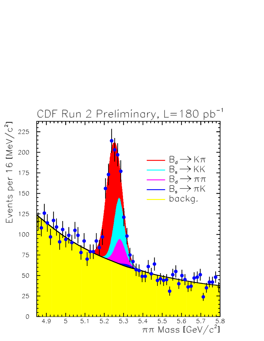
Figure 1: $\pi\pi$ invariant mass distribution of $B_{s(d)}\to h^{+}h^{{}^{\prime}-}$ candidates.

Figure 2: Monte Carlo distribution of $M_{\pi\pi}$ versus $(1-\frac{p_{1}}{p_{2}})*q_{1}$ for different $B_{s(d)}\to h^{+}h^{{}^{\prime}-}$ channels.

With this, we obtain the first observation of $B_{s}\rightarrow K^{+}K^{-}$:

$\frac{f_{s}~{}R(B_{s}\rightarrow K^{+}K^{-})}{f_{d}~{}BR(B_{d}\rightarrow K\pi)}=0.46\pm 0.08(stat.)\pm 0.07(syst.)$,

and a big improvement in the limit on $B_{s}\rightarrow K^{+}\pi^{-}$:

$BR(B_{s}\rightarrow K\pi)<0.08*BR(B_{d}\rightarrow K\pi)*(f_{s}/f_{d})$

@90% C.L.

In the $B_{d}$ sector we obtain:

$A_{CP}(B_{d}\rightarrow K\pi)=\frac{N(B_{d}\rightarrow K^{+}\pi^{-})-N(\overline{B}_{d}\rightarrow K^{-}\pi^{+})}{N(B_{d}\rightarrow K^{+}\pi^{-})+N(\overline{B}_{d}\rightarrow K^{-}\pi^{+})}=-0.022\pm 0.078(stat.)\pm 0.012(syst.)$,

being this result perfectly compatible with $B$ factories. It is important to notice that $A_{CP}$ systematics are at the level of Babar and Belle experiments, and we expect to reach Y(4S) precision on the statistical uncertainty with the current sample on tape as well.

3 $\Delta\Gamma_{s}/\Gamma_{s}$ Measurement in $B_{s}\rightarrow J/\Psi\phi$ Decays

In order to measure the decay width difference $\Delta\Gamma_{s}$ we need to disantangle the heavy and light $B_{s}$ mass eigentstates and measure their lifetimes separately. In the $B_{s}$ system CP violation is supposed to be small ($\delta\phi_{s}\approx 0$). Thus the heavy and light $B_{s}$ mass eigenstates directly correspond to the CP even and CP odd eigenstates. So the separation of the $B_{s}$ mass eigenstates can be done by identifying the CP even and CP odd contributions.

Generally final states are mixtures of CP even and odd states, but for pseudoscalar particles where the $B_{s}$ decays into two vector particles such as the $J/\Psi$ and the $\phi$ it is possible to disantangle the CP even and CP odd eigenstates by an angular analysis. The decay amplitude decomposes into 3 linear polarization states with the amplitudes $A_{0},A_{\parallel}$ and $A_{\perp}$ with

$$|A_{0}|^{2}+|A_{\parallel}|^{2}+|A_{\perp}|^{2}=1.$$ (1)

$A_{0}$ and $A_{\parallel}$ correspond to the S and D wave and are therefore the CP even contribution, while $A_{\perp}$ corresponds to the P wave and thus to the CP odd component.

It is possible to measure the lifetimes of the heavy and light $B_{s}$ mass eigenstate, by fitting at the same time for the angular distributions and for the lifetimes.

A similar angular analysis has been already performed by the BABAR and BELLE experiments in the $B_{d}\rightarrow J/\Psi K^{*0}$ mode. This mode has as well been studied at the Tevatron as a cross check for the $B_{s}\rightarrow J/\Psi\phi$ analysis.

In order to perform this analysis first of all a $B_{s}\rightarrow J/\Psi\phi$ signal has to be established. Both experiments have measured the $B_{s}$ mass and lifetime, as shown in Fig. 3 for the D$\oslash$ analysis, where the lifetime $\tau_{s}$ is measured with respect to $\tau_{d}$ from the topological similar decay $B_{d}\rightarrow J/\Psi K^{*0}$.

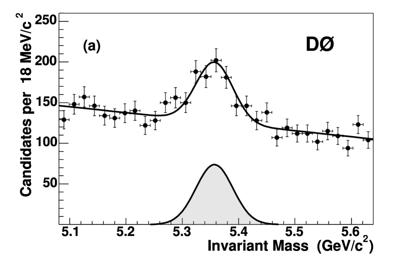
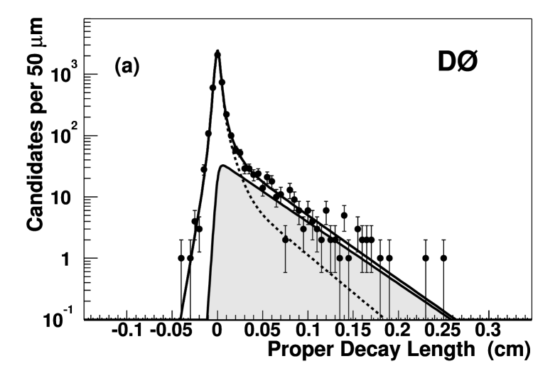
Figure 3: Mass (left) and average lifetime (right) distributions of $B_{s}\rightarrow J/\Psi\phi$ candidates from D$\oslash$.

The angular analysis has been performed in the transversity basis in the $J/\Psi$ rest-frame which is introduced in Fig. 4. The fit projections of the common fit of the both lifetimes and the angular distributions for the CDF analysis and for the D$\oslash$ analysis are shown in Fig. 4.

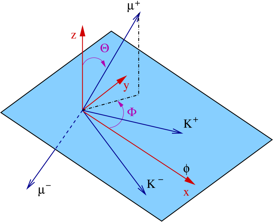
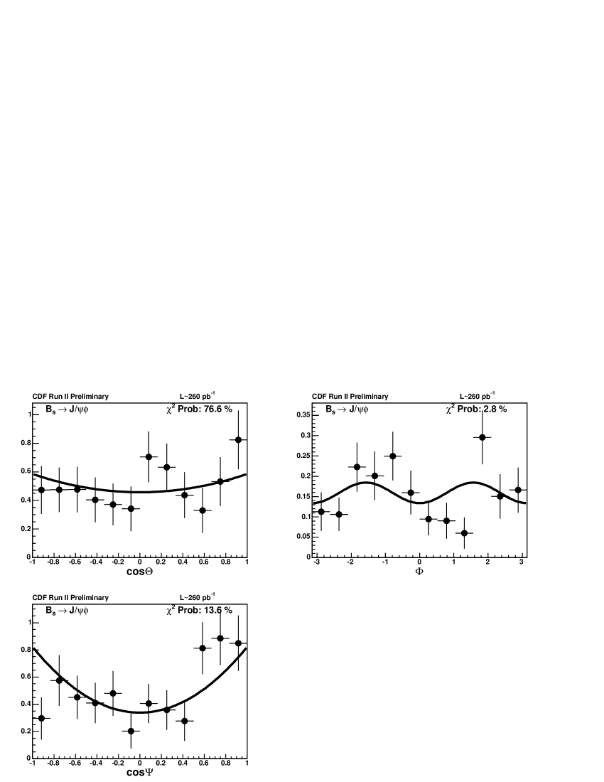
Figure 4: Definition of the transversity frame and the transversity angles (left) and fit projections of the common fit of both lifetime and angular distributions from the CDF analysis (right).

The results of both experiments are summarized in Tab. 1 and Fig. 5. The combined result slightly favors high values of $\Delta m_{s}$, but is currently statistically limited. The systematic uncertainties are very small, thus this is a precise measurement ones more data is available.

Table 1: $\Delta\Gamma_{s}/\Gamma_{s}$ results from CDF and D$\oslash$.

Experiment	$\Delta\Gamma_{s}/\Gamma_{s}$	$<\tau>$ (ps)	$\tau_{L}$ (ps)	$\tau_{H}$ (ps)
CDF	$0.65^{+0.25}_{-0.33}$	$1.40^{+0.15}_{-0.13}$	$1.05^{+0.16}_{-0.13}$	$2.07^{+0.58}_{-0.46}$
D$\oslash$	$0.21^{+0.33}_{-0.45}$	$1.39^{+0.15}_{-0.16}$	$1.23^{+0.16}_{-0.13}$	$1.52^{+0.39}_{-0.43}$

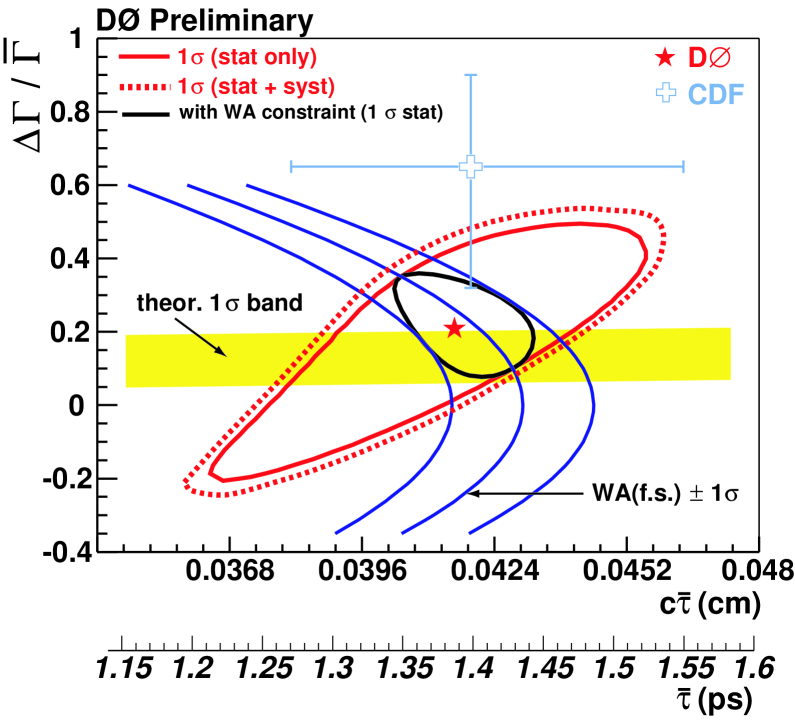
Figure 5: $\Delta\Gamma_{s}/\Gamma_{s}$ versus c$<\tau>$ results from CDF and D$\oslash$.

4 $B_{s}$ Mixing

The probability that a $B$ meson decays at proper time $t$ and has or has not already mixed to the $\bar{B}$ state is given by:

$$P_{unmix}(t) \approx \frac{1}{2}(1+\cos\Delta mt),$$ (2)

$$P_{mix}(t) \approx \frac{1}{2}(1-\cos\Delta mt).$$ (3)

The canonical $B$ mixing analysis, in which oscillations are observed and the mixing frequency, $\Delta m$, is measured, proceeds as follows. The $B$ meson flavor at the time of its decay is determined by exclusive reconstruction of the final state. The proper time, $t=m_{B}L/pc$, at which the decay occurred is determined by measuring the decay length, $L$, and the $B$ momentum, $p$. Finally the production flavor must be tagged in order to classify the decay as being mixed or unmixed at the time of its decay.

Oscillation manifests itself in a time dependence of, for example, the mixed asymmetry:

$${\cal A}_{mix}(t)=\frac{N_{mixed}(t)-N_{unmixed}(t)}{N_{mixed}(t)+N_{unmixed}(t)}=-\cos\Delta mt$$ (4)

In practice, the production flavor will be correctly tagged with a probability $P_{tag}$, which is significantly smaller than one, but larger than one half (which corresponds to a random tag). The measured mixing asymmetry in terms of dilution, $\cal D$, is

$${\cal A}^{meas}_{mix}(t)={\cal D}{\cal A}_{mix}=-{\cal D}\cos\Delta mt$$ (5)

where ${\cal D}=2P_{tag}-1$.

First of all a good proper decay time resolution, which is specially important in order to resolve high $\Delta m_{s}$ mixing frequency.

The second important ingredient for a mixing analysis is the flavor tagging. As the examined decays are flavor specific modes the decay flavor can be determined via the decay products. But for the production flavor additional information from the event has to be evaluated in order to tag the event. A good and well measured tagging performance is needed to set a limit on $\Delta m_{s}$.

The last component are the $B_{s}$ candidates. Sufficient statistic is need to be sensitive to high mixing frequencies.

4.1 Flavor Tagging

There are two different kinds of flavor tagging algorithms, opposite side tagging (OST) and same side tagging (SST), which are illustrated in Fig. 6. OST algorithms use the fact that b quarks are mostly produced in $b\bar{b}$ pairs, therefore the flavor of the second (opposite side) $b$ can be used to determine the flavor of the $b$ quark on the signal side.

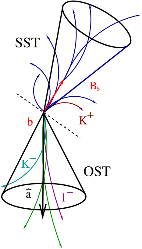
Figure 6: Left: Sketch of different tagging algorithms; Right: Same-side kaon tagging.

4.1.1 Jet-Charge Tagging

The average charge of an opposite side $b$-jet is weakly correlated to the charge of the opposite $b$ quark and can thus be used to determine the opposite side $b$ flavor. The main challenge of this tagger is to select the $b$-jet. Information of a displaced vertex or displaced tracks in the jet help to identify $b$-jets. This tagging algorithm has a very high tagging efficiency, but the dilution is relatively low. By separating sets of tagged events of different qualities e.g. how $b$ like the jet is, it is possible to increase the overall tagging performance.

4.1.2 Soft-Lepton-Tagging

In 20 % of cases the opposite semileptonic $b$ decays either into an electron or a muon ($b\rightarrow l^{-}X$). The charge of the lepton is correlated to the charge of the decaying $B$ meson. Depending on the type of the $B$ meson there is a certain probability of oscillation between production and decay (0 % for $B^{\pm}$, 17.5 % for $B_{d}$ and 50 % for $B_{s}$). Therefore this tagging algorithm already contains an intrinsic dilution. Another potential source of miss-tag is the transition of the $b$ quark into a $c$ quark, which then forms a $D$ meson and subsequently decays semileptonically ($\bar{b}\rightarrow\bar{c}\rightarrow l^{-}X$). Due to the different decay length and momentum distribution of $B$ and $D$ meson decays this source of miss-tag can mostly be eliminated.

4.1.3 Same-Side-Tagging

During fragmentation and the formation of the $B_{s/d}$ meson there is a left over $\bar{s}/\bar{d}$ quark which is likely to form a $K^{+}/\pi^{+}$ (Fig. 6). So if there is a near by charged particle, which is additionally identified as a kaon/pion, it is quite likely that it is the leading fragmentation track and its charge is then correlated to the flavor of the $B_{s/d}$ meson. While the performance of the opposite side tagger does not depend on the flavor of the $B$ on the signal side the SST performance depends on the signal fragmentation processes. Therefore the opposite side performance can be measured in $B_{d}$ mixing and can then be used for setting a limit on the $B_{s}$ mixing frequency. But for using the SST for a limit on $\Delta m_{s}$ we have to heavily rely on Monte Carlo simulation. The SST potentially has the best tagger performance, but before using it for a limit, fragmentation processes have to be carefully understood.

4.2 $\Delta m_{d}$ Measurement and Calibration of Taggers

For setting a limit on $\Delta m_{s}$ the knowledge of the tagger performance is crucial. Therefore it has to be measured in kinematically similar $B_{d}$ and $B^{+}$ samples.

The $\Delta m_{s}$ and $\Delta m_{d}$ analysis is a complex fit with up to 500 parameters which combine several $B$ flavor and several decay modes, various different taggers and deals with complex templates for mass and lifetime fits for various sources of background. Therefore the measurement of $\Delta m_{d}$ is beside the calibration of the opposite side taggers very important to test and trust the fitter framework, although the actual $\Delta m_{d}$ result at the Tevatron is not competitive with the $B$ factories.

Both CDF and D$\oslash$ have demonstrated that the whole machinery is working, being $\Delta m_{d}$ measurements compatible with the PDG average value of $0.510\pm 0.004$ $ps^{-1}$ pdg . The combined tagging performance of the opposite-side taggers is about 1.5-2%.

An example of the fitted asymmetry using the opposite side muon tagger on the semileptonic decay modes from D$\oslash$ is displayed in Fig. 7.

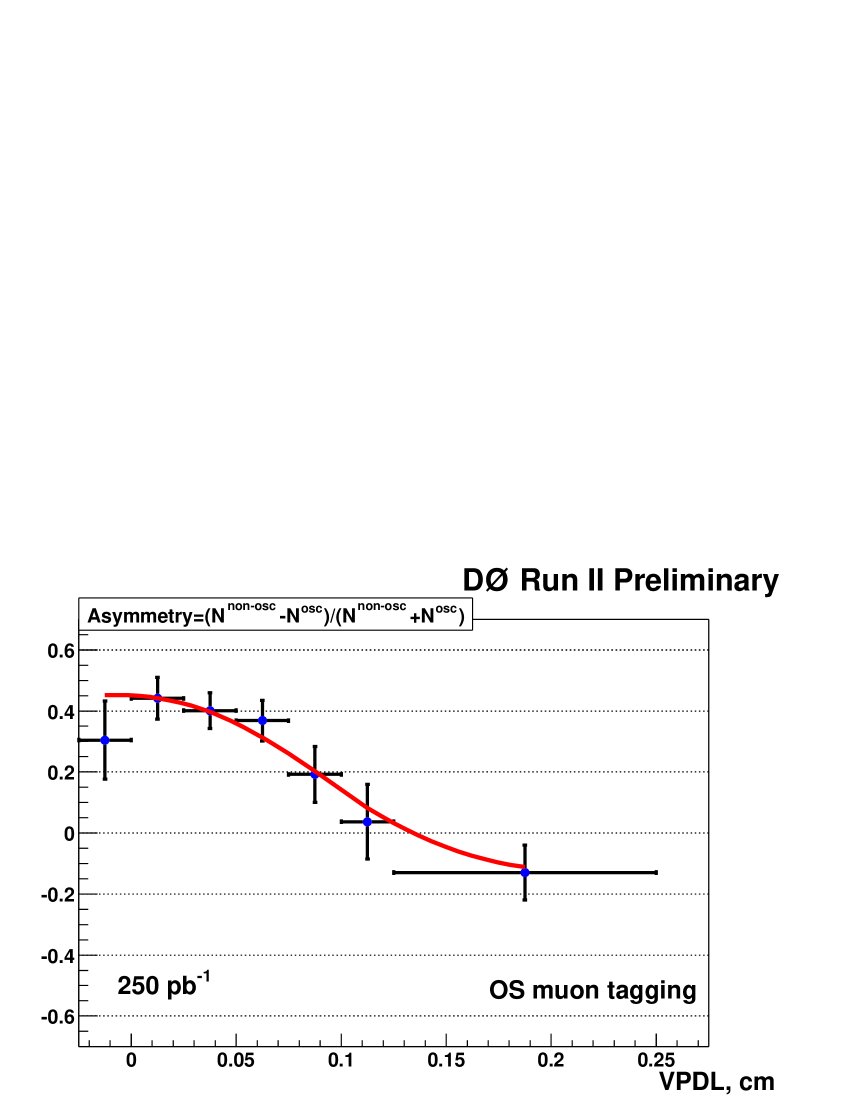
Figure 7: Asymmetry fit projection for $\Delta m_{d}$ using opposite side muon tagger in semileptonic decays from D$\oslash$.

4.3 Amplitude Scan

An alternative method for studying neutral $B$ meson oscillations is the so called “amplitude scan”, which is explained in detail in Reference moser . The likelihood term describing the tagged proper decay time of a neutral $B$ meson is modified by including an additional parameter multiplying the cosine, the so-called amplitude $A$.

The signal oscillation term in the likelihood of the $\Delta m$ thus becomes

$${\cal L}\propto\frac{1\pm A{\cal D}\cos(\Delta mt)}{2}$$ (6)

The parameter $A$ is left free in the fit while ${\cal D}$ is supposed to be known and fixed in the scan. The method involves performing one such $A$-fit for each value of the parameter $\Delta m$, which is fixed at each step; in the case of infinite statistics, optimal resolution and perfect tagger parameterization and calibration, one would expect $A$ to be unit for the true oscillation frequency and zero for the remaining of the probed spectrum. In practice, the output of the procedure is accordingly a list of fitted values ($A$, $\sigma_{A}$) for each $\Delta m$ hypothesis. Such a $\Delta m$ hypothesis is excluded to a $95$% confidence level in case the following relation is observed, $A+1.645\cdot\sigma_{A}<1$.

The sensitivity of a mixing measurement is defined as the lowest $\Delta m$ value for which $1.645\cdot\sigma_{A}=1$.

The amplitude method will be employed in the ensuing $B_{s}$ mixing analysis. One of its main advantages is the fact that it allows easy combination among different measurements and experiments.

The plot shown in Figure 8 is obtained when the method is applied to the hadronic $B_{d}$ samples of the CDF experiment, using the exclusively combined opposite side tagging algorithms.

The expected compatibility of the measured amplitude with unit in the vicinity of the true frequency, $\Delta m_{d}=0.5~{}$ps^-1, is confirmed.

However, we observe the expected increase in the amplitude uncertainty for higher oscillation frequency hypotheses. This is equivalent to saying that the significance is reduced with increasing frequency.

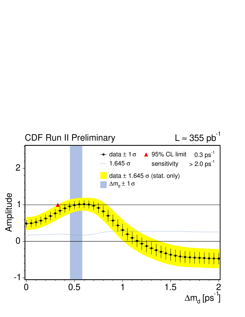
Figure 8: Amplitude scan for $\Delta m_{d}$ in hadronic decay modes (CDF). The scan is compatible with 1 around the result of the actual $\Delta m_{d}$ fit.

4.4 Reconstructed $B_{s}$ Decays

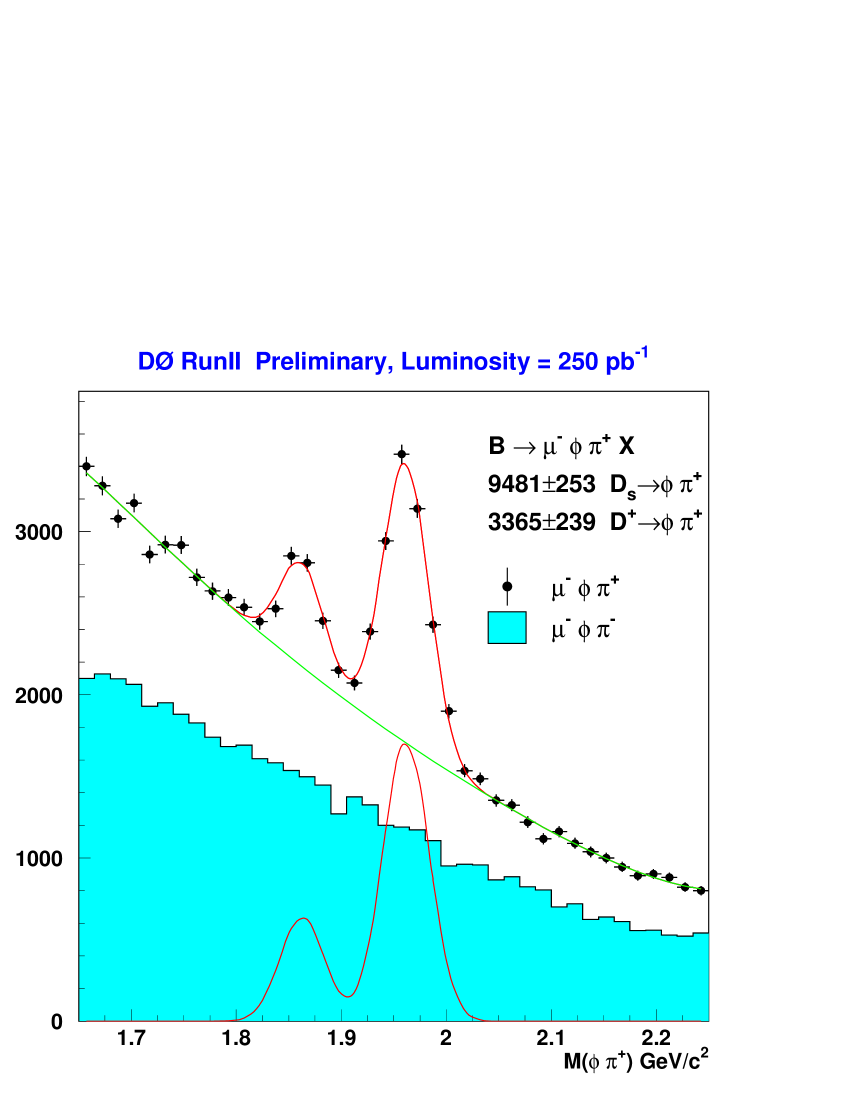
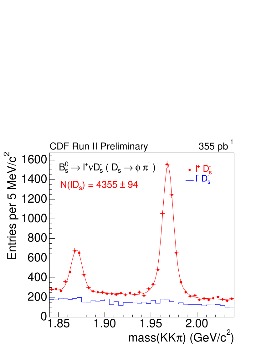
Figure 9: Reconstructed semileptonic $B_{s}\rightarrow lXD_{s},(D_{s}\rightarrow\phi\pi)$ candidates from D$\oslash$ (left) and CDF (right).

D$\oslash$ exploits the high statistics muon trigger to study semileptonic $B_{s}$ decays. Several thousands candidates have been reconstructed in the $B_{s}\rightarrow\mu XD_{s},(D_{s}\rightarrow\phi\pi)$ mode. Additionally D$\oslash$ is also working on reconstructing $B_{s}\rightarrow\mu XD_{s},(D_{s}\rightarrow K^{*0}K)$ candidates and on reconstructing fully hadronic $B_{s}$ decays on the non trigger side in this sample.

CDF performs the $B_{s}$ mixing analysis using both fully reconstructed $B_{s}$ decays ($B_{s}\rightarrow D_{s}\pi$) obtained by the two track trigger and semileptonic decays ($B_{s}\rightarrow\ell XD_{s}$) collected in the lepton+displaced track trigger. In both cases the $D_{s}$ is reconstructed in the $D_{s}\rightarrow\phi\pi$, $D_{s}\rightarrow K^{*0}K$ and $D_{s}\rightarrow\pi\pi\pi$ modes.

Fig. 9 shows the reconstructed semileptonic $B_{s}\rightarrow lXD_{s}$, $(D_{s}\rightarrow\phi\pi)$ candidates from D$\oslash$ and CDF.

4.5 First $\Delta m_{s}$ Limits in Run II

Finally, an amplitude scan, repeating the Likelihood fit for the amplitude $A$ for different values of $\Delta m_{s}$, was performed in both D$\oslash$ and CDF. The results of the amplitude scans are shown in Fig. 10 and 11. The amplitude scan yields a $\Delta m_{s}$ sensitivity of 8.4(4.6) $ps^{-1}$ and a lower exclusion limit of 7.9(5.0) $ps^{-1}$ is set on the value of $\Delta m_{s}$ at a 95% confidence level in CDF (D$\oslash$).

Those results are good enough for the first round of the analysis, but there is still a huge room for improvements in the near future.

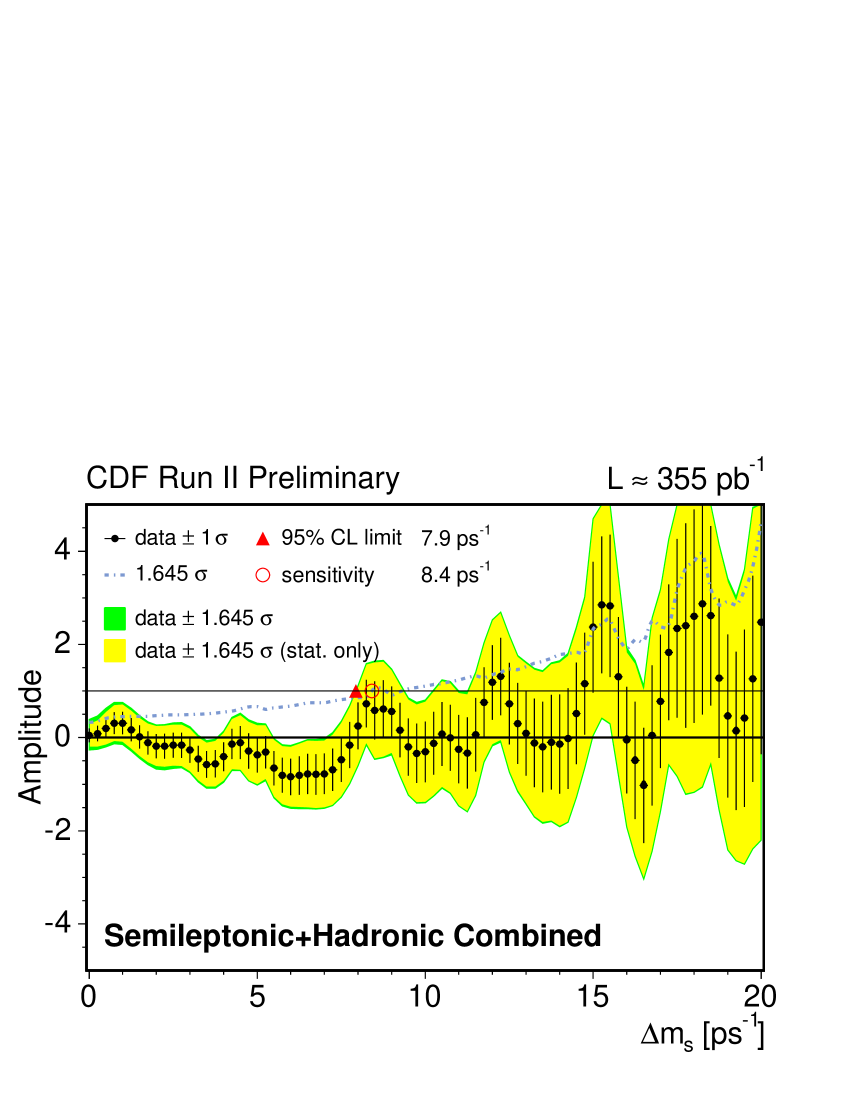
Figure 10: Combined amplitude scan from CDF. The black dots represent the fitted amplitude with their respective statistical errors for each value of $\Delta m_{s}$. The yellow region indicates 1.645 $\sigma$ using statistical errors only while the green band includes combined statistical and systematic errors. The measurement is dominated by statistical uncertainties. Note, neighboring points are statistically correlated.

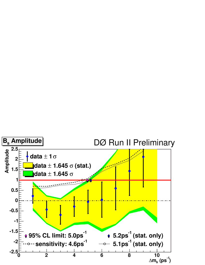
Figure 11: Combined amplitude scan from D$\oslash$.

5 Conclusions

The large amount of data collected by the CDF and D$\oslash$ experiments are improving our knowledge about $B_{s}$ mesons. A few selected topics have been discussed in this paper. The measurement of the decay width difference $\Delta\Gamma_{s}$ of the heavy and light $B_{s}$ mass eigenstate is especially sensitive to high $\Delta m_{s}$ values. The $B_{s}$ mixing analysis is sensitive to lower values. Together they have the potential to cover the hole range of possible $\Delta m_{s}$ values in the Standard Model and as well beyond.

References

-
(1)
The CDF Collaboration,
http://www-cdf.fnal.gov/physics/new/bottom/bottom.html. -
(2)
The D Collaboration,
http://www-d0.fnal.gov/Run2Physics/WWW/results/b.htm. - (3) R. Blair et al., The CDF-II detector: Technical Design report, FERMILAB-PUB-96-390-E (1996).
- (4) A. Abachi et al, The D upgrade: The detector and its physics, FERMILAB-PUB-96-357-E (1996).
-
(5)
S. Eidelman et al. [Particle Data Group],
http://pdg.web.cern.ch/pdg. - (6) H.G. Moser, A.Roussrie, Mathematical methods for oscillation analysed, NIM A384 (1997), 491-505.