Measurement of the branching fractions for $J/\psi\rightarrow\gamma\pi^{0}$, $\gamma\eta$ and $\gamma\eta^{\prime}$

Abstract

The decay modes $J/\psi\rightarrow\gamma\pi^{0},\gamma\eta$ and $\gamma\eta^{\prime}$ are analyzed using a data sample of 58 million $J/\psi$ decays collected with the BESII detector at BEPC. The branching fractions are determined to be: $Br(J/\psi\rightarrow\gamma\pi^{0})=(3.13^{+0.65}_{-0.44})\times 10^{-5}$, $Br(J/\psi\rightarrow\gamma\eta)=(11.23\pm 0.89)\times 10^{-4}$, and $Br(J/\psi\rightarrow\gamma\eta^{\prime})=(5.55\pm 0.44)\times 10^{-3}$, where the errors are combined statistical and systematic errors. The ratio of partial widths $\Gamma(J/\psi\rightarrow\gamma\eta^{\prime})/\Gamma(J/\psi\rightarrow\gamma\eta)$ is measured to be $4.94\pm 0.40$, and the singlet-octet pseudoscalar mixing angle of $\eta-\eta^{\prime}$ system is determined to be $\theta_{P}=(-22.08\pm 0.81)^{\circ}$.

I INTRODUCTION

In flavor-$SU(3)$, the $\pi^{0}$, $\eta$ and $\eta^{\prime}$ mesons belong to the same pseudoscalar nonet. The physical states $\eta$ and $\eta^{\prime}$ are related to the $SU_{f}(3)$-octet state $\eta_{8}$ and the $SU_{f}(3)$-singlet state $\eta_{1}$, via the usual mixing formulae:

$$\eta=\eta_{8}\cos\theta_{P}-\eta_{1}\sin\theta_{P},$$

$$\eta^{\prime}=\eta_{8}\sin\theta_{P}+\eta_{1}\cos\theta_{P},$$

where $\theta_{P}$ is the pseudoscalar mixing angle theo ; mixing . The conventional estimate of $\eta-\eta^{\prime}$ mixing uses the quadratic mass matrix

$$M^{2}=\left(\begin{array}[]{cc}M^{2}_{88}&M^{2}_{18}\\ M^{2}_{18}&M^{2}_{11}\end{array}\right),$$

where $M^{2}_{88}=\frac{1}{3}(4m^{2}_{K}-m^{2}_{\pi})$ is given by the Gell-Mann-Okubo mass formula. Diagonalization of this matrix gives

$$\tan^{2}\theta_{P}=\frac{M^{2}_{88}-m^{2}_{\eta}}{m^{2}_{\eta^{\prime}}-M^{2}_{88}}\Longrightarrow\theta_{P}\approx-10^{\circ}.$$

With a linear mass matrix and the linear Gell-Mann-Okubo mass formula $M_{88}=\frac{1}{3}(4m_{K}-m_{\pi})$, $\theta_{P}$ is computed to be about $-24^{\circ}$ mixing .

The mixing angle has been measured experimentally in different ways, and the value is around $-20^{\circ}$ mixing . One of these measurements is based on $J/\psi$ radiative decays. In the limit where the OZI rule and $SU_{f}(3)$ symmetry are exact, one gets thetap1

$$R=\frac{\Gamma(J/\psi\rightarrow\gamma\eta^{\prime})}{\Gamma(J/\psi\rightarrow\gamma\eta)}=(\frac{p_{\eta^{\prime}}}{p_{\eta}})^{3}\cdot{\cot^{2}\theta_{P}},$$

where $p_{\eta}$ and $p_{\eta^{\prime}}$ are the momenta of $\eta$ and $\eta^{\prime}$ in the $J/\psi$ Center of Mass System (CMS).

The first-order perturbation theory pertu1 ; pertu2 expression for the partial width $\Gamma(J/\psi\rightarrow\gamma+pseudoscalar)$ is

$$\Gamma(J/\psi\rightarrow\gamma+P)=\frac{1}{6}(\frac{2}{3})^{2}\alpha^{4}_{s}\alpha Q^{2}_{c}\frac{1}{M^{3}_{J/\psi}}(\frac{4R_{J/\psi}(0)}{\sqrt{4\pi M_{J/\psi}}})^{2}(\frac{4R_{P}(0)}{\sqrt{4\pi M_{P}}})^{2}x|H^{P}(x)|^{2}.$$

Here $R_{J/\psi}(0)$ and $R_{P}(0)$ are the wave functions at the origin of the $J/\psi$ and the pseudoscalar with mass $M_{P}$, and $Q_{c}$ is the charge of the charmed quark. The pseudoscalar helicity amplitude $H^{P}(x)$ depends on $x=1-(\frac{M_{P}}{M_{J/\psi}})^{2}$; numerically $x|H^{P}(x)|\approx 55$ for $M_{P}=m_{\eta^{\prime}}$. $R_{J/\psi}(0)$ and $R_{P}(0)$ can be determined from the $J/\psi\rightarrow e^{+}e^{-}$ and $P\rightarrow\gamma\gamma$ partial decay widths, respectively. Using the lowest-order QCD formula for $\alpha_{s}$, the $J/\psi\rightarrow\gamma\eta^{\prime}$ decay width is calculated to be 213 eV, which is in agreement with the experimentally measured value. The value of $\Gamma(J/\psi\rightarrow\gamma\eta)$ determined from the same formula disagrees with measurements. Some models that assign a small admixture of $\eta$ and $\eta^{\prime}$ to other states have been proposed to explain the large value of the ratio $R=\Gamma(J/\psi\rightarrow\gamma\eta^{\prime})/\Gamma(J/\psi\rightarrow\gamma\eta)$. For example, Ref. ratio1 , which assigns small $c\bar{c}$ contribution from $\eta_{c}$ in the $\eta$ and $\eta^{\prime}$ wave functions, predicts $R=3.9$; Ref. ratio2 gives a value of $R=5.1$ by considering some admixture of the $\iota(1440)$ to the $\eta$ and $\eta^{\prime}$. A precision measurement of $R$ could distinguish between these mixing models, as well as provide a determination of the mixing angle $\theta_{P}$. Experimental measurements of $Br(J/\psi\rightarrow\gamma\eta)$ and $Br(J/\psi\rightarrow\gamma\eta^{\prime})$ were reported by the DESY-Heidelberg group DESY , the Crystal Ball CBAL , MarkIII MARK3 and DM2 DM2 .

The decay $J/\psi\rightarrow\gamma\pi^{0}$ is suppressed because the photon can only be radiated from the final state quarks. This branching fraction was measured by DASP DASP and Crystal Ball CBAL ; the average of the measurements, $(3.9\pm 1.3)\times 10^{-5}$ PDG04 , is in agreement with the VMD prediction $3.3\times 10^{-5}$ VMD . In contrast, the QCD multipole expansion theory mutipole predicts a value of $1\times 10^{-6}$.

In this paper, $J/\psi\rightarrow\gamma\pi^{0}$ is studied using $\pi^{0}\rightarrow\gamma\gamma$ decay, $J/\psi\rightarrow\gamma\eta$ is measured using $\eta\rightarrow\gamma\gamma$ and $\eta\rightarrow\pi^{0}\pi^{+}\pi^{-}$ with $\pi^{0}\rightarrow\gamma\gamma$, and $J/\psi\rightarrow\gamma\eta^{\prime}$ is studied using $\eta^{\prime}\rightarrow\gamma\gamma$, $\eta^{\prime}\rightarrow\gamma\pi^{+}\pi^{-}$ and $\eta^{\prime}\rightarrow\eta\pi^{+}\pi^{-}$ with $\eta\rightarrow\gamma\gamma$. The analyses use a data sample that contains $58\times 10^{6}$ $J/\psi$ decays collected with the updated BEijing Spectrometer (BESII) operating at the Beijing Electron Positron Collider (BEPC).

II BES DETECTOR AND MONTE CARLO SIMULATION

BESII is a large solid-angle magnetic spectrometer that is described in detail in Ref. bes2 . The momentum of charged particles is measured in a 40-layer cylindrical main drift chamber (MDC) with a momentum resolution of $\sigma_{p}$/p=$1.78\%\sqrt{1+p^{2}}$ ($p$ in GeV/c). Particle identification is accomplished using specific ionization ($dE/dx$) measurements in the drift chamber and time-of-flight (TOF) information from a barrel-like array of 48 scintillation counters. The $dE/dx$ resolution is $\sigma_{dE/dx}\simeq 8.0\%$; the TOF resolution for Bhabha events is $\sigma_{TOF}=180$ ps. Radially outside of the time-of-flight counters is a 12-radiation-length barrel shower counter (BSC) comprised of gas tubes interleaved with lead sheets. The BSC measures the energy and direction of photons with resolutions of $\sigma_{E}/E\simeq 21\%\sqrt{E}$ ($E$ in GeV), $\sigma_{\phi}=7.9$ mrad, and $\sigma_{z}=2.3$ cm. The iron flux-return of the magnet is instrumented with three double layers of proportional counters that are used to identify muons.

A GEANT3-based Monte Carlo simulation package simbes , which simulates the detector response including interactions of secondary particles in the detector material, is used to determine detection efficiencies and mass resolutions, optimize selection criteria, and estimate backgrounds. Reasonable agreement between data and MC simulation is observed for various calibration channels, including $e^{+}e^{-}\to(\gamma)e^{+}e^{-}$, $e^{+}e^{-}\to(\gamma)\mu^{+}\mu^{-}$, $J/\psi\to p\bar{p}$, $J/\psi\to\rho\pi$ and $\psi(2S)\to\pi^{+}\pi^{-}J/\psi$, $J/\psi\to l^{+}l^{-}$.

III DATA ANALYSIS

III.1 $J/\psi\rightarrow\gamma\gamma\gamma$

In the $J/\psi\rightarrow\gamma\gamma\gamma$ decay mode, there are no charged tracks in the final states. Each candidate event is required to have three and only three photon candidates; the MC indicates that the number of these decays that produce final states with more than three photon candidates is negligible. A photon candidate is defined as a cluster in the BSC with an energy deposit of more than 50 MeV, and with an angle between the development direction of the cluster and the direction from the interaction point to the first hit layer of the BSC that is less than 20^∘. If two clusters have an opening angle that is less than 10^∘ or have an invariant mass that is less than 50 MeV$/c^{2}$, the lower energy cluster is regarded as a remnant from the other and not a separate photon candidate. A kinematic fit that conserves energy and momentum is applied to the three photon candidates, and $\chi^{2}\leq 20$ is required. We also require $|\cos\theta_{v}|<0.8$ and $\theta_{min}>6^{\circ}$, where $\theta_{v}$ is the polar angle of a decay photon in the pseudoscalar’s CMS (shown in Fig. 1a), and $\theta_{min}$ is the minimum angle between any two of the three photon candidates (shown in Fig. 1b). This rejects background from the continuum $e^{+}e^{-}\rightarrow\gamma\gamma(\gamma)$ process.

(a)                                              (b)

Figure 1: Distribution of (a) $\cos\theta_{v}$ and (b) $\theta_{min}$. The open histograms are $J/\psi$ data, the shaded histograms are background from $e^{+}e^{-}\rightarrow\gamma\gamma(\gamma)$, and the dashed lines are simulated $J/\psi\rightarrow\gamma\pi^{0}\rightarrow\gamma\gamma\gamma$ events (not normalized).

III.1.1 $J/\psi\rightarrow\gamma\pi^{0},\pi^{0}\rightarrow\gamma\gamma$

Figure 2 shows the invariant mass distribution in the $\pi^{0}$ mass region of the two photon candidates that have the smallest opening angle. A peak at the $\pi^{0}$ mass is evident.

Figure 2: Invariant mass distribution of the $\gamma\gamma$ with smallest opening angle for $J/\psi\rightarrow\gamma\gamma\gamma$ candidate events. The solid squares with error bars are data, the histogram is the best fit described in the text, and the dashed line is the background.

From MC studies, background channels that produce a peak in the $\pi^{0}$ signal region come mainly from channels with $5\gamma$ final states, such as $J/\psi\rightarrow\gamma\pi^{0}\pi^{0}$, via the $f_{2}(1270)$, $f_{0}(2100)$ etc. ($J/\psi\rightarrow 4\gamma$s violates C-parity). These background sources are studied using events where the number of photon candidates in the event is four. Four photon events are selected and subjected to a four-constraint kinematic fit to $J/\psi\rightarrow\gamma\gamma\gamma$, using any three of the four photons; the three-photon combination with the smallest $\chi^{2}$ is selected for the background study. Figure 3 shows the invariant mass distribution for the two photons with the smallest opening angle from four-photon events. A peak is observed in the $\pi^{0}$ mass region that agrees with expectations from MC simulations that include all known modes that produce $5\gamma$ final states. However, since the known background channels do not account for the level of the observed background in the data sample, a scale factor is introduced to scale the MC background predictions for fits to the distribution in Fig. 2. The scale factor depends strongly on which intermediate states are considered for $J/\psi\rightarrow 5\gamma$ decays; the difference between the scale factors determined from different channels is treated as a systematic uncertainty of the background subtraction.

Figure 2 is fit with a MC-simulated $J/\psi\rightarrow\gamma\pi^{0}$ histogram for the signal, a MC-simulated $J/\psi\rightarrow 5\gamma$ background shape, as well as a shape of MC simulated phase space for other sources of backgrounds. The number of $\gamma\pi^{0}$ events determined from the fit is $586\pm 51$. The MC-determined detection efficiency for $J/\psi\rightarrow\gamma\pi^{0},\pi^{0}\rightarrow\gamma\gamma$ is $\varepsilon=(32.80\pm 0.21)$%, where the error comes from the limited statistics of the MC sample.

Figure 3: The invariant mass distribution of $\gamma\gamma$ pairs with the smallest opening angle in $J/\psi\rightarrow\gamma\gamma\gamma$ events selected from the four photon event sample.

III.1.2 $J/\psi\rightarrow\gamma\eta,\eta\rightarrow\gamma\gamma$

Figure 4 shows the invariant mass distribution of the two photon candidates with the smallest opening angle in the $\eta$ mass region, where an $\eta$ peak is evident.

Figure 4: Invariant mass distribution of the $\gamma\gamma$ with the smallest opening angle of $J/\psi\rightarrow\gamma\gamma\gamma$ candidates. Solid squares with error bars are data, the histogram is the fit result, and the dashed line is the background.

The $\gamma\gamma$ invariant mass distribution of Fig. 4 is fit with a histogram from MC-simulated $J/\psi\rightarrow\gamma\eta,\eta\rightarrow\gamma\gamma$ events and a second order Legendre polynomial background function. The fit yields a signal of 9096$\pm$133 $\eta$s. The MC-determined detection efficiency is $\varepsilon=(36.33\pm 0.22)\%$.

III.1.3 $J/\psi\rightarrow\gamma\eta^{\prime},\eta^{\prime}\rightarrow\gamma\gamma$

Since the momentum of the $\eta^{\prime}$ is lower than that of the $\pi^{0}$ and $\eta$ in $J/\psi$ radiative decays, the angle between the two $\eta^{\prime}$ decay photons is not small enough to be useful for distinguishing them from the radiative photon. For this channel, the mass distribution of the three $\gamma\gamma$ combinations for each event are plotted in Fig. 5, where an $\eta^{\prime}$ signal is evident above a smooth background due to wrong $\gamma\gamma$ combinations plus other background sources.

Figure 5: The $\gamma\gamma$ invariant mass distribution for $J/\psi\rightarrow\gamma\gamma\gamma$ candidate events (three entries per event). The solid squares with error bars indicate data, the histogram is the fit result, and the dashed line is the non-combinatorial background.

A fit to the data points, with the MC simulated mass distribution for the $J/\psi\rightarrow\gamma\eta^{\prime},\eta^{\prime}\rightarrow\gamma\gamma$ decay including combinatorial background for the signal and a second order Legendre polynomial for background between 0.8 and 1.2 $\hbox{GeV}/c^{2}$, yields $2982\pm 101$ entries. Since all the $\gamma\gamma$ combinations are plotted in the $M_{\gamma\gamma}$ distribution, the combinatorial background is included in the entries for both data and MC simulation. The efficiency for signal $J/\psi\rightarrow\gamma\eta^{\prime},\eta^{\prime}\rightarrow\gamma\gamma$ entries is $(40.30\pm 0.22)\%$. The combinatorial background is about $20\%$ for both data and MC simulation, and they cancel out when the $N^{obs}$ is divided by the efficiency $40.30\%$ in the branching fraction calculation.

III.2 $J/\psi\rightarrow\gamma\gamma\gamma\pi^{+}\pi^{-}$

In this final states, there are two charged particles $\pi^{+}$ and $\pi^{-}$ and three photons. Candidate events are required to satisfy the following common selection criteria:

1. Two good charged tracks with net charge zero. Each track must have a good helix fit, a transverse momentum larger than 60 MeV/c, and $|\cos\theta|<0.8$, where $\theta$ is the polar angle of the track, and must originate from the interaction region.

2. At least one charged track is identified as a $\pi$, satisfying $\chi^{2}_{PID}(\pi)<\chi^{2}_{PID}(K)$ and $\chi^{2}_{PID}(\pi)<\chi^{2}_{PID}(p)$, where $\chi^{2}_{PID}=\chi^{2}_{dE/dx}+\chi^{2}_{TOF}$ is determined using both $dE/dx$ and TOF information.

3. At least three photon candidates are required. The photon identification is similar to that used in the $J/\psi\rightarrow\gamma\gamma\gamma$ analysis, except that the angle between a cluster and any other cluster must be greater than $18^{\circ}$, and the angle between the cluster and any charged track must be greater than $8^{\circ}$. These differences reflect different sources of fake photons.

4. A four-constraint kinematic fit is applied to all three-photon combinations plus the two charged tracks assuming $J/\psi\rightarrow\gamma\gamma\gamma\pi^{+}\pi^{-}$. The three-photon combination with the smallest $\chi^{2}$ is selected, and the $\chi^{2}$ of the kinematic fit is required to be less than 20.

The events that survive these selection criteria with an invariant mass in the range $M_{\gamma\gamma\pi^{+}\pi^{-}}\leq 1.2\hbox{GeV}/c^{2}$ are assumed to come from either $\eta$ or $\eta^{\prime}$ decays, and the other photon is considered to be the radiative photon. Figure 6 shows a scatterplot of $M_{\gamma\gamma}$ versus $M_{\gamma\gamma\pi^{+}\pi^{-}}$ for the selected events. Clear $\eta$ and $\eta^{\prime}$ signals corresponding to $\eta\rightarrow\pi^{0}\pi^{+}\pi^{-},\pi^{0}\rightarrow\gamma\gamma$, and $\eta^{\prime}\rightarrow\eta\pi^{+}\pi^{-},\eta\rightarrow\gamma\gamma$ are observed.

Figure 6: Scatterplot of $M_{\gamma\gamma}$ versus $M_{\gamma\gamma\pi^{+}\pi^{-}}$ for the $J/\psi\rightarrow\gamma\gamma\gamma\pi^{+}\pi^{-}$ candidates.

III.2.1 $J/\psi\rightarrow\gamma\eta,\eta\rightarrow\pi^{0}\pi^{+}\pi^{-}$

After the requirement that the $\gamma\gamma$ invariant mass is in the $\pi^{0}$ mass region ($M_{\gamma\gamma}\in[0.088,0.182]~{}\hbox{GeV}/c^{2}$, $\pm 3\sigma$), a clear $\eta$ signal is evident in the $\gamma\gamma\pi^{+}\pi^{-}$ invariant mass distribution shown in Fig. 7.

Figure 7: The $\gamma\gamma\pi^{+}\pi^{-}$ invariant mass distribution for $J/\psi\rightarrow\gamma\gamma\gamma\pi^{+}\pi^{-}$ candidates that satisfy the requirement $M_{\gamma\gamma}\in[0.088,0.182]~{}\hbox{GeV}/c^{2}$. The solid squares with error bars indicate the data, the histogram is the fit result, and the dashed line is the background.

The simulated $M_{\gamma\gamma\pi^{+}\pi^{-}}$ mass distribution from the signal MC and a second-order Legendre polynomial are used to fit the $\gamma\gamma\pi^{+}\pi^{-}$ invariant mass distribution. The fit gives $1885\pm 58$ $\eta$ events. The MC-determined detection efficiency for $J/\psi\rightarrow\gamma\eta,\eta\rightarrow\pi^{0}\pi^{+}\pi^{-}$, and $\pi^{0}\rightarrow\gamma\gamma$ is $\varepsilon=(12.25\pm 0.15)\%$.

III.2.2 $J/\psi\rightarrow\gamma\eta^{\prime},\eta^{\prime}\rightarrow\eta\pi^{+}\pi^{-}$

The $\gamma\gamma\pi^{+}\pi^{-}$ invariant mass distribution for events with $\gamma\gamma$ mass within $3\sigma$ of the $\eta$ mass ($M_{\gamma\gamma}\in[0.484,0.612]~{}\hbox{GeV}/c^{2}$), is shown in Fig. 8.

Figure 8: The $\gamma\gamma\pi^{+}\pi^{-}$ invariant mass distribution for events with $\gamma\gamma$ mass in the $\eta$ mass region ($M_{\gamma\gamma}\in[0.484,0.612]~{}\hbox{GeV}/c^{2}$). The solid squares with error bars indicate data, the histogram is the fit result, and the dashed line is the background.

A similar fit as for $\eta\rightarrow\pi^{0}\pi^{+}\pi^{-}$ yields $8572\pm 131$ $\eta^{\prime}$ events; the MC-determined detection efficiency for $J/\psi\rightarrow\gamma\eta^{\prime},\eta^{\prime}\rightarrow\eta\pi^{+}\pi^{-}$, and $\eta\rightarrow\gamma\gamma$ is $\varepsilon=(16.10\pm 0.12)\%$.

III.3 $J/\psi\rightarrow\gamma\gamma\pi^{+}\pi^{-}$

$J/\psi\rightarrow\gamma\eta^{\prime}$ is also studied using the $\eta^{\prime}\rightarrow\gamma\pi^{+}\pi^{-}$ decay channel. For this study, the $\pi^{\pm}$ and photon selection requirements are the same as used for the $J/\psi\rightarrow\gamma\gamma\gamma\pi^{+}\pi^{-}$ final state, and the event selection is similar, except that here at least two photons are required in the event. The photons and charged tracks are kinematically fitted to $J/\psi\rightarrow\gamma\gamma\pi^{+}\pi^{-}$ assuming four-momentum conservation, and $\chi^{2}\leq 20$ is required. When there are more than two photons, the kinematic fit is repeated using all possible photon combinations, and the one with the smallest $\chi^{2}$ is kept. The photon with the higher energy is considered to be the radiative photon from the $J/\psi$ decay. Figure 9 shows the invariant mass distribution of $\gamma\pi^{+}\pi^{-}$ for the candidate events where an $\eta^{\prime}$ signal is evident.

Figure 9: The $\gamma\pi^{+}\pi^{-}$ invariant mass distribution for selected $J/\psi\rightarrow\gamma\gamma\pi^{+}\pi^{-}$ events. The solid squares with error bars indicate data, the histogram is the fit result, and the dashed line is the background.

Figure 9 shows the result of a fit to the $\gamma\pi^{+}\pi^{-}$ invariant mass distribution that follows a similar procedure as that for the fit to the $\gamma\gamma\pi^{+}\pi^{-}$ distribution of the previous section. The fit yields $23243\pm 229$ $\eta^{\prime}$ signal events. The MC-determined detection efficiency for $J/\psi\rightarrow\gamma\eta^{\prime},\eta^{\prime}\rightarrow\gamma\pi^{+}\pi^{-}$ is $\varepsilon=(25.02\pm 0.10)\%$.

IV SYSTEMATIC ERRORS

Systematic errors in the branching fraction measurements mainly originate from photon identification (ID), MDC tracking efficiency, particle ID, kinematic fitting, mass resolution, $\pi^{0}$ reconstruction, and parameterizations of background shapes.

IV.1 Photon identification

The efficiency for photon ID is discussed in Ref. lism . It is found that the relative efficiency difference between data and MC simulation for high energy photon detection is about 0.8% per photon, while for low energy photons, the difference is around 2% per photon. Since the energy of the radiative photon in $J/\psi\rightarrow\gamma\pi^{0},\gamma\eta$, and $\gamma\eta^{\prime}$ is high, and the energies of the photons from pseudoscalar particle decays are low, the total systematic error due to photon ID is taken as $(0.8+2.0n)\%$, where $n$ is the number of photons from the pseudoscalar particle decay.

IV.2 MDC tracking

The MDC tracking efficiency is studied in Ref. simbes . It is found that there is a 2.0% relative difference per track between data and MC simulation. For the channels in this analysis that have two charged tracks, a 4% systematic error on the MDC tracking efficiency is assigned.

IV.3 Particle ID

A clean charged $\pi$ sample obtained from $J/\psi\rightarrow\rho\pi$ without the use of particle ID is used to study data-MC differences between particle ID efficiencies for different momentum ranges. Since only one of the two charged tracks is required to be identified as a pion, the MC simulates data rather well; it is found that the MC simulation agrees with data within 0.2% for both $J/\psi\rightarrow\gamma\gamma\gamma\pi^{+}\pi^{-}$ and $J/\psi\rightarrow\gamma\gamma\pi^{+}\pi^{-}$ modes.

IV.4 Kinematic fit

Samples of $J/\psi\rightarrow\rho\pi$ and $e^{+}e^{-}\rightarrow\gamma\gamma$ events selected without using kinematic fits are used to study the systematic error associated with the four-constraint kinematic fit. For the $\chi^{2}\leq 20$ criteria, the difference of kinematic fit efficiencies between data and MC simulation is less than 1.2% for $\rho\pi$, and 2.4% for $e^{+}e^{-}\rightarrow\gamma\gamma$. Extrapolating these differences to the channels reported here, we conservatively assign a 4% systematic error to the kinematic fit efficiency.

IV.5 Different mass resolution between MC and DATA

There is a slight difference of the mass resolution between MC simulation and data. When the histogram shape of invariant mass distribution from MC simulation is used to fit the invariant mass distribution of data, it introduces some systematic error. The high statistics decay channels $J/\psi\rightarrow\gamma\eta,\eta\rightarrow\gamma\gamma$, $J/\psi\rightarrow\gamma\eta^{\prime},\eta^{\prime}\rightarrow\gamma\gamma\pi^{+}\pi^{-}$ and $J/\psi\rightarrow\gamma\eta^{\prime},\eta^{\prime}\rightarrow\gamma\pi^{+}\pi^{-}$ are used to study this source of systematic error. For these channels, we allow the mass resolution to vary in the fit to the invariant mass distributions, and we also determine the number of signal events by subtracting side-band-estimated backgrounds. The resulting branching fractions change by at most 1.6%, 0.1%, and 0.6% for $J/\psi\rightarrow\gamma\eta,\eta\rightarrow\gamma\gamma$, $J/\psi\rightarrow\gamma\eta^{\prime},\eta^{\prime}\rightarrow\eta\pi^{+}\pi^{-}$, and $J/\psi\rightarrow\gamma\eta^{\prime},\eta^{\prime}\rightarrow\gamma\pi^{+}\pi^{-}$ respectively. We assign 1.6%, 0.1% and 0.6% as the systematic errors due to mass resolution uncertainties for the $J/\psi\rightarrow\gamma\gamma\gamma$, $J/\psi\rightarrow\gamma\gamma\gamma\pi^{+}\pi^{-}$ and $J/\psi\rightarrow\gamma\gamma\pi^{+}\pi^{-}$ decay modes, respectively.

IV.6 Reconstruction of $\pi^{0}$

In $J/\psi\rightarrow\gamma\pi^{0}$, the $\pi^{0}$ momentum is high and the angle between the two decay photons is small. As a result, it is possible for the two photons to merge into a single BSC cluster. According to a study reported in Ref. xinbo , the systematic error associated with 1.5 GeV $\pi^{0}$ reconstruction is 0.83%. The effect on low energy $\pi^{0}$s or $\eta$s is small enough to be neglected.

IV.7 Background shape

For the $J/\psi\rightarrow\gamma\pi^{0}$ mode, the background estimate based on the four photon event sample has a large uncertainty. Fits using MC-determined background shapes from different background channels yield different numbers of signal events; the corresponding changes in the branching fractions range between ${}^{+16.4}_{-6.8}\%$. The largest difference is taken as the systematic error. Different order Legendre polynomials are used to fit the mass spectra for the other decay modes, and the differences between these fits and those used to get the numbers of signal events are used as the systematic error due to background parameterization. Different fitting ranges are also used in the fit, and the differences are included in the systematic error. The uncertainty due to the background shape and fitting range is less than 2%.

IV.8 Branching fractions of the secondary decays

The branching fractions of decay from $\pi^{0},\eta$ and $\eta^{\prime}$ are taken from the PDG PDG04 ; the uncertainties are included in the measurement errors of the reported branching fractions.

IV.9 The number of $J/\psi$ events

The total number of $J/\psi$ events, determined from the 4-prong data sample, is $(57.7\pm 2.72)\times 10^{6}$. The 4.72% relative error is taken as a systematic error fangss .

IV.10 Total systematic error

Table I summarizes the systematic errors from all sources for each mode. We assume all the sources are independent and add them in quadrature; the resulting total systematic errors are ${}^{+18.3}_{-10.6}\%$, $8.1\%$, $10.6\%$, $9.3\%$, $9.5\%$, and $8.7\%$ for $J/\psi\rightarrow\gamma\pi^{0}\rightarrow\gamma\gamma\gamma$, $J/\psi\rightarrow\gamma\eta\rightarrow\gamma\gamma\gamma$, $J/\psi\rightarrow\gamma\eta^{\prime}\rightarrow\gamma\gamma\gamma$, $J/\psi\rightarrow\gamma\eta\rightarrow\gamma\gamma\gamma\pi^{+}\pi^{-}$, $J/\psi\rightarrow\gamma\eta^{\prime}\rightarrow\gamma\gamma\gamma\pi^{+}\pi^{-}$, and $J/\psi\rightarrow\gamma\eta^{\prime}\rightarrow\gamma\gamma\pi^{+}\pi^{-}$, respectively.

Table 1: Summary of the systematic errors (%).

Sources	$\pi^{0}\rightarrow\gamma\gamma$	$\eta\rightarrow\gamma\gamma$	$\eta^{\prime}\rightarrow\gamma\gamma$	$\eta\rightarrow\pi^{0}\pi^{+}\pi^{-}$	$\eta^{\prime}\rightarrow\eta\pi^{+}\pi^{-}$	$\eta^{\prime}\rightarrow\gamma\pi^{+}\pi^{-}$
Photon ID	4.8	4.8	4.8	4.8	4.8	2.8
Tracking	-	-	-	4.0	4.0	4.0
Particle ID	-	-	-	0.2	0.2	0.2
Kinematic fit	4.0	4.0	4.0	4.0	4.0	4.0
Mass resolution	1.6	1.6	1.6	0.1	0.1	0.6
$\pi^{0}$ reconstruction	0.83	-	-	-	-	-
Background shape	${}^{+16.4}_{-6.8}$	0.73	1.8	1.7	0.5	0.2
Branching fraction used	0.04	0.66	6.61	1.77	3.45	3.39
Number of $J/\psi$	4.72	4.72	4.72	4.72	4.72	4.72
Statistic of MC sample	0.64	0.61	0.55	1.23	0.75	0.40
Total error	${}^{+18.3}_{-10.6}$	8.1	10.6	9.3	9.5	8.7

V RESULTS AND DISCUSSION

The branching fractions of $J/\psi$ decays are determined from the relation

$$Br(J/\psi\rightarrow\gamma P)=\frac{N^{obs}(J/\psi\rightarrow\gamma P\rightarrow\gamma Y)}{N^{J/\psi}\cdot Br(P\rightarrow Y)\cdot\varepsilon(J/\psi\rightarrow\gamma P\rightarrow\gamma Y)},$$

where $P$ is either $\pi^{0}$, $\eta$, or $\eta^{\prime}$, $Y$ is the pseudoscalar decay final state, and $Br(P\rightarrow Y)$ is the branching fraction of the pseudoscalar decays into final state $Y$. The results of $Br(J/\psi\rightarrow\gamma P)$ are listed in Table II.

The branching fractions of $J/\psi\rightarrow\gamma\eta$, $J/\psi\rightarrow\gamma\eta^{\prime}$ measured from different decay modes are consistent with each other within the statistical fluctuations and uncommon systematic errors. The measurements from the different modes are, therefore, combined using a standard weighted least-squares procedure taking into consideration the correlations between the measurements; the mean value and the error are calculated by:

$$\bar{x}\pm\delta\bar{x}=\frac{\sum_{j}{x_{j}}\cdot(\sum_{i}{\omega_{ij}})}{\sum_{i}\sum_{j}{\omega_{ij}}}\pm\sqrt{\frac{1}{\sum_{i}\sum_{j}{\omega_{ij}}}}.$$

Here $\omega_{ij}$ is the element of the weighted matrix $W=V^{-1}_{x}$, where $V_{x}$ is the covariance matrix calculated according to the systematic errors listed in Table I. For $J/\psi\rightarrow\gamma\eta$, the correlation coefficient between $\eta\rightarrow\gamma\gamma$ and $\eta\rightarrow\gamma\gamma\pi^{+}\pi^{-}$ is $\rho(1,2)=0.553$; for $J/\psi\rightarrow\gamma\eta^{\prime}$, the correlation coefficients between $\eta^{\prime}\rightarrow\gamma\gamma$, $\eta^{\prime}\rightarrow\gamma\pi^{+}\pi^{-}$ and $\eta^{\prime}\rightarrow\gamma\gamma\pi^{+}\pi^{-}$ are $\rho(1,2)=0.296$, $\rho(1,3)=0.404$ and $\rho(2,3)=0.703$. The weighted averages of BESII measurements and the PDG PDG04 values are listed in Table II.

Table 2: Branching fractions of $J/\psi\rightarrow\gamma\pi^{0},\gamma\eta$ and $\gamma\eta^{\prime}$.

Decay mode		BESII	BESII combined	PDG PDG04
$\gamma\pi^{0}$	$\pi^{0}\rightarrow\gamma\gamma$	$(3.13\pm 0.28^{+0.58}_{-0.34})\times 10^{-5}$	$(3.13^{+0.65}_{-0.44})\times 10^{-5}$	$(3.9\pm 1.3)\times 10^{-5}$
$\gamma\eta$	$\eta\rightarrow\gamma\gamma$	$(11.00\pm 0.16\pm 0.90)\times 10^{-4}$	$(11.23\pm 0.89)\times 10^{-4}$	$(8.6\pm 0.8)\times 10^{-4}$
	$\eta\rightarrow\pi^{0}\pi^{+}\pi^{-}$	$(11.94\pm 0.37\pm 1.11)\times 10^{-4}$
	$\eta^{\prime}\rightarrow\gamma\gamma$	$(6.05\pm 0.21\pm 0.65)\times 10^{-3}$
$\gamma\eta^{\prime}$	$\eta^{\prime}\rightarrow\gamma\rho$	$(5.46\pm 0.06\pm 0.48)\times 10^{-3}$	$(5.55\pm 0.44)\times 10^{-3}$	$(4.31\pm 0.30)\times 10^{-3}$
	$\eta^{\prime}\rightarrow\eta\pi^{+}\pi^{-}$	$(5.28\pm 0.08\pm 0.51)\times 10^{-3}$

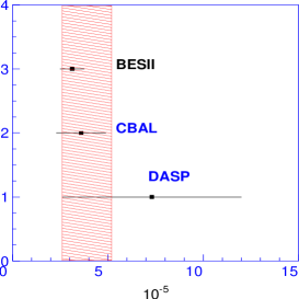
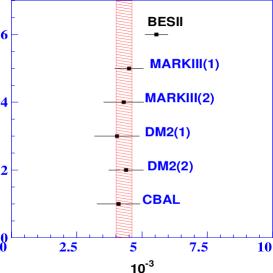
Figure 10: Comparisons of $Br(J/\psi\rightarrow\gamma\pi^{0})$, $Br(J/\psi\rightarrow\gamma\eta)$ and $Br(J/\psi\rightarrow\gamma\eta^{\prime})$ between BESII and previous measurements PDG04 . The shaded regions are the world averages from the PDG PDG04 .

Figure 10 shows the comparisons between the measurements in this paper and those from previous measurements DESY ; CBAL ; MARK3 ; DM2 ; DASP . Our measurement of $Br(J/\psi\rightarrow\gamma\pi^{0})$ agrees with those of Crystal Ball CBAL and DASP DASP within the large errors of the previous measurements, and has much improved precision. Our measurement’s lower central value may be because background channels that produce a peak in the signal region have been considered. Our measurements of $Br(J/\psi\rightarrow\gamma\eta)$ and $Br(J/\psi\rightarrow\gamma\eta^{\prime})$ are higher than the PDG world average PDG04 , and have better precision than the previous measurements DESY ; CBAL ; MARK3 ; DM2 .

The results listed in Table II also allow us calculate the relative branching fractions for $\eta$ and $\eta^{\prime}$ decays; considering the common errors in the measurements, one gets

$$\frac{Br(\eta^{\prime}\rightarrow\gamma\gamma)}{Br(\eta^{\prime}\rightarrow\gamma\pi^{+}\pi^{-})}=\frac{Br(J/\psi\rightarrow\gamma\eta^{\prime},\eta^{\prime}\rightarrow\gamma\gamma)}{Br(J/\psi\rightarrow\gamma\eta^{\prime},\eta^{\prime}\rightarrow\gamma\pi^{+}\pi^{-})}=0.080\pm 0.008,$$

$$\frac{Br(\eta^{\prime}\rightarrow\eta\pi^{+}\pi^{-})}{Br(\eta^{\prime}\rightarrow\gamma\pi^{+}\pi^{-})}=\frac{Br(J/\psi\rightarrow\gamma\eta^{\prime},\eta^{\prime}\rightarrow\eta\pi^{+}\pi^{-})}{Br(J/\psi\rightarrow\gamma\eta^{\prime},\eta^{\prime}\rightarrow\gamma\pi^{+}\pi^{-})}=1.45\pm 0.07,$$

$$\frac{Br(\eta\rightarrow\gamma\gamma)}{Br(\eta\rightarrow\pi^{0}\pi^{+}\pi^{-})}=\frac{Br(J/\psi\rightarrow\gamma\eta,\eta\rightarrow\gamma\gamma)}{Br(J/\psi\rightarrow\gamma\eta,\eta\rightarrow\pi^{0}\pi^{+}\pi^{-})}=1.61\pm 0.14.$$

The correlation coefficients between denominator and numerator in above equations are 0.419, 0.859 and 0.575 respectively. The world averages PDG04 of the same ratios are $0.072\pm 0.006$, $1.50\pm 0.08$ and $1.75\pm 0.04$ respectively. The agreement is quite good.

If both the OZI rule and the $SU_{f}(3)$ symmetry are exact, it is expected that thetap1 :

$$R=\frac{\Gamma(J/\psi\rightarrow\gamma\eta^{\prime})}{\Gamma(J/\psi\rightarrow\gamma\eta)}=(\frac{P_{\eta^{\prime}}}{P_{\eta}})^{3}\cdot{\cot^{2}\theta_{P}}.$$

Using $Br(J/\psi\rightarrow\gamma\eta)$ and $Br(J/\psi\rightarrow\gamma\eta^{\prime})$ in this analysis, one obtains

$$R=4.94\pm 0.40,$$

$$|\theta_{P}|=(22.08\pm 0.81)^{\circ},$$

where the common errors have been considered in the ratio calculation. Comparing with the mixing models with states other than $\eta$ and $\eta^{\prime}$, the measurement of $R$ agrees with the prediction of $R=5.1$ ratio2 within one standard deviation, while it deviates from $R=3.9$ ratio1 by more than 3 standard deviations. According to the theoretical calculation of Ref. mixing , the value of $\theta_{P}$ is negative, in which case its value is $\theta_{P}=(-22.08\pm 0.81)^{\circ}$.

VI SUMMARY

Using 58 million $J/\psi$ events collected by BESII, the branching fractions of $J/\psi$ decays into a photon and a pseudoscalar meson are measured as $Br(J/\psi\rightarrow\gamma\pi^{0})=(3.13^{+0.65}_{-0.44})\times 10^{-5}$, $Br(J/\psi\rightarrow\gamma\eta)=(11.23\pm 0.89)\times 10^{-4}$, and $Br(J/\psi\rightarrow\gamma\eta^{\prime})=(5.55\pm 0.44)\times 10^{-3}$. The results are compared to $\eta$ and $\eta^{\prime}$ mixing models.

VII Acknowledgment

The BES collaboration thanks the staff of BEPC for their hard efforts. This work is supported in part by the National Natural Science Foundation of China under contracts Nos. 10491300, 10225524, 10225525, 10425523, the Chinese Academy of Sciences under contract No. KJ 95T-03, the 100 Talents Program of CAS under Contract Nos. U-11, U-24, U-25, and the Knowledge Innovation Project of CAS under Contract Nos. U-602, U-34 (IHEP), the National Natural Science Foundation of China under Contract No. 10225522 (Tsinghua University), and the Department of Energy under Contract No.DE-FG02-04ER41291 (U Hawaii).

References

(1) J. F. Donoghue, B. R. Holstein and Y. -C. R. Lin, Phys.
Rev. Lett. 55, 2766 (1985); R. Escribano and J. -M. Frre, hep-ph/0501072 (2005).
(2) F. J. Gilman and R. Kauffman, Phys. Rev. D36, 2761 (1987).
(3) R. N. Cahn and M. S. Chanowitz, Phys. Lett. B59, 277 (1975).
(4) J. G. Körner, J. H. Kühn, M. Krammer, H. Schneider, Nucl. Phys. B229, 115 (1983).
(5) B. Guberina and J. H. Kühn, Nuovo Cim. Lett. 32, 295 (1981).
(6) S. Eidelman et al.(Particle Data Group), Phys. Lett. B592, 1 (2004).
(7) H. Fritsch and J. D. Jackson, Phys. Lett. B66, 365 (1977).
(8) H. Yu, High Energy Phys. & Nucl. Phys. 12, 754 (1988) (in Chinese).
(9) W. Bartel et al., Phys. Lett. B66, 489 (1977).
(10) E. D. Bloom, C. Peck, ARNS 33, 143 (1983).
(11) T. Bolton et al., Phys. Rev. Lett. 69, 1328 (1992).
(12) J. E. Augustin et al., Phys. Rev. D42, 10 (1990).
(13) W. Braunschweig et al., Phys. Lett. B67, 243 (1977).
(14) V. L. Chernyak and A. R. Zhitnitsky, Phys. Rept. 112, 173 (1984).
(15) Y. P. Kuang, Phys. Rev. D42, 2300 (1990).
(16) BES Collab., J. Z. Bai et al., Nucl. Instrum. Methods A458, 627 (2001).
(17) BES Collab., M. Ablikim et al., physics/0503001, to be published in Nucl. Instrum. Methods A.
(18) S. M. Li et al., High Energy Phys. & Nucl.Phys., 28, 859 (2004) (Chinese Edition).
(19) BES Collab., M. Ablikim et al., Phys. Rev. D71, 072006 (2005).
(20) S. S. Fang et al.,
High Energy Phys. & Nucl. Phys. 27, 277 (2003) (in Chinese).