Study of the decay asymmetry parameter and CP violation parameter in the $\Lambda_{c}^{+}\to\Lambda\pi^{+}$ decay.

Abstract

Using data from the FOCUS (E831) experiment at Fermilab, we present a new measurement of the weak decay-asymmetry parameter $\alpha_{\Lambda_{c}}$ in $\Lambda_{c}^{+}\to\Lambda\pi^{+}$ decay. Comparing particle with antiparticle decays, we obtain the first measurement of the CP violation parameter $\mathcal{A}\equiv{\alpha_{\Lambda_{c}}+\alpha_{\overline{\Lambda_{c}}}\over\alpha_{\Lambda_{c}}-\alpha_{\overline{\Lambda_{c}}}}$. We obtain $\alpha_{\Lambda_{c}}=-0.78\pm 0.16\pm 0.13$ and $\mathcal{A}=-0.07\pm 0.19\pm 0.12$ where errors are statistical and systematic.

The FOCUS Collaboration

1 Introduction

Parity violation in the weak decay of a spin $1\over 2$ hyperon into a spin $1\over 2$ baryon and a pseudoscalar meson is well known. An example is $\Lambda\to p\pi^{-}$ [1], where the angular distribution of the proton in the $\Lambda$ rest frame is given by

$${dW\over d\cos\theta}={1\over 2}(1+P\alpha_{\Lambda}\cos\theta)$$ (1)

where P is the polarization of $\Lambda$ along the $z$ direction, $\theta$ is the polar angle and $\alpha_{\Lambda}$ is the weak decay-asymmetry parameter. The latter is defined as

$$\alpha_{\Lambda}\equiv{2{\mathcal{R}e}(A_{+}^{*}A_{-})\over|A_{+}|^{2}+|A_{-}|^{2}}$$ (2)

where $A_{+}$ and $A_{-}$ are the parity-even and parity-odd decay amplitudes. In a non-relativistic picture, they correspond to the $L=0$ and $L=1$ orbital angular momenta of the proton-$\pi$ system respectively.

Eqn. (1) can be generalized for the case of a baryon double decay chain like $\Lambda_{c}^{+}\to\Lambda\pi^{+}$ with $\Lambda\to p\pi^{-}$ in which each baryon weak decay is a ${1\over 2}^{+}\to{1\over 2}^{+}+{0^{-}}$ process. If the $\Lambda_{c}^{+}$ is produced unpolarized, Eqn. (1) for the $\Lambda$ decay becomes

$${dW\over d\cos\theta}={1\over 2}(1+\alpha_{\Lambda_{c}}\alpha_{\Lambda}\cos\theta)$$ (3)

where $\alpha_{\Lambda_{c}}$ is the weak-decay asymmetry parameter of the $\Lambda_{c}^{+}\to\Lambda\pi^{+}$ process and $\theta$ is the helicity angle of the proton in the $\Lambda$ rest frame, i.e. it is the supplement of the angle (i.e. $\pi$ minus the angle) in the $\Lambda$ rest frame between the proton and the direction of the $\Lambda_{c}^{+}$. For this decay of the $\Lambda_{c}^{+}$, this is the same as the angle, in the $\Lambda$ rest frame, between the proton and the $\pi^{+}$ decay product of the $\Lambda_{c}^{+}$, and the supplement of this angle is used in this analysis. The distribution of the helicity angle, $\theta$, determines the product $\alpha_{\Lambda_{c}}\alpha_{\Lambda}$, and, since $\alpha_{\Lambda}$ is known, (in this analysis we assume $\alpha_{\Lambda}=-\alpha_{\overline{\Lambda}}=0.642\pm 0.013$ [2]), one can extract $\alpha_{\Lambda_{c}}$.

If CP were conserved exactly, $\alpha_{\Lambda_{c}}$ of the $\Lambda_{c}^{+}\to\Lambda\pi^{+}$ process would be the negative of $\alpha_{\overline{\Lambda_{c}}}$ in $\overline{\Lambda}{}_{c}^{-}\to{\overline{\Lambda}}\pi^{-}$ decay. Just as with the $\Lambda$ decay, there is the possibility of CP violation in $\Lambda_{c}^{+}$ decay (a weak decay with possible final state interactions). In this paper we 1) measure $\alpha_{\Lambda_{c}}$ and $\alpha_{\overline{\Lambda_{c}}}$ separately, 2) use them for the first measurement of the CP asymmetry parameter

$$\mathcal{A}\equiv{\alpha_{\Lambda_{c}}+\alpha_{\overline{\Lambda_{c}}}\over\alpha_{\Lambda_{c}}-\alpha_{\overline{\Lambda_{c}}}}$$ (4)

and 3) having established that the difference is negligible within our errors, combine the data for particle and antiparticle decays to obtain the best value of the asymmetry parameter. In this analysis the $\Lambda_{c}^{+}$ is assumed to be unpolarized and thus the $\Lambda$ longitudinal polarization (polarization along the $\Lambda$ momentum direction in the $\Lambda_{c}^{+}$ rest frame) is $\alpha_{\Lambda_{c}}$. As discussed later, if the polarization is the maximum allowed in our data, the effect on our measurement is negligible.

FOCUS is a charm photoproduction experiment, an upgraded version of E687 [3], which collected data during the 1996–97 fixed target run at Fermilab. Electron and positron beams obtained from the $800~{}\mathrm{GeV/c}$ Tevatron proton beam produce, by means of bremsstrahlung, a photon beam (with typically $300~{}\mathrm{GeV}$ endpoint energy) which interacts with a segmented BeO target [4]. The mean photon energy for triggered events is $\sim 180~{}\mathrm{GeV}$. A system of three multicell threshold Čerenkov counters is used to perform the charged particle identification, separating kaons from pions up to $60~{}\mathrm{GeV}/c$ of momentum. Two systems of silicon microvertex detectors are used to track particles: the first system consists of 4 planes of microstrips interleaved with the experimental target [3, 5] and the second system consists of 12 planes of microstrips located downstream of the target. These detectors provide high resolution in the transverse plane (approximately $9~{}\mu\mathrm{m}$ on the track position), allowing the identification and separation of charm production and decay vertices. The charged particle momentum is determined by measuring the deflections in two magnets of opposite polarity through five stations of multiwire proportional chambers.

2 Analysis of the decay mode $\Lambda_{c}^{+}\to\Lambda\pi^{+}$ + charge conjugate.

Unless explicitly stated otherwise, both the particle and its charge conjugate are implied. The selection of $\Lambda_{c}^{+}$ events begins with the identification of $\Lambda$ candidates on the basis of vertexing and loose Ĉerenkov cuts on the pion and proton decay particles as described in detail elsewhere [6]. The tracks of these charged daughters are used to form the decay vertex of the $\Lambda$ and to determine its flight direction and momentum. The momentum of the $\Lambda$ is used together with the momentum of a $\pi^{+}$ (or with the momentum of a $\pi^{-}$ in the case of a $\overline{\Lambda}$) to find the $\Lambda_{c}^{+}$ (${\overline{\Lambda}}{}_{c}^{-}$ ) vertex and its momentum. We call this pion $\tilde{\pi}$. The $\Lambda$’s used in this analysis can be divided into two categories: the $\sim 10$% which decayed before the microstrip detector and the large majority that decayed after the first microstrip plane. For the former, both the $\Lambda$ decay vertex and the momentum vector are measured precisely by the FOCUS spectrometer; for the latter only the momentum vector is measured precisely. Thus different algorithms are used to find the $\Lambda_{c}^{+}$ decay vertex and the production vertex in these interactions. For the $\Lambda$’s decaying upstream of the the microstrips, both the vertex position and the direction of the $\Lambda$ are used in combination with a fully reconstructed $\tilde{\pi}$ track. The confidence level that the $\tilde{\pi}$ and the $\Lambda$ originated from the same $\Lambda_{c}^{+}$ decay vertex is computed and required to be $>1$%. The $\Lambda_{c}^{+}$ candidate decay vertex and momentum are calculated and used as the initial track for a candidate driven vertex algorithm [3]. The momentum and position of the resultant $\Lambda_{c}^{+}$ candidate are used as a seed track to intersect the other reconstructed tracks and to search for a production vertex. The confidence level of this vertex is required to be greater than 1%.

For the $\Lambda$’s decaying downstream of the first plane of the microstrip, we use the momentum information from the $\Lambda$ decay and the silicon track of $\tilde{\pi}$ to form a candidate $\Lambda_{c}^{+}$ momentum vector. This vector and the $\tilde{\pi}$ track form a plane in which the momentum vector of the candidate $\Lambda_{c}^{+}$ lies. The transverse distance from this plane is calculated for candidate production vertices which are formed by at least two other silicon tracks and the confidence level that the vertex lies in the plane is computed. The $\Lambda_{c}^{+}$ trajectory is forced to originate at this production vertex and the confidence level that it verticizes with $\tilde{\pi}$ is calculated. If this confidence level is greater than 2%, this vertex is taken as the decay vertex of the $\Lambda_{c}^{+}$ and used with the $\Lambda_{c}^{+}$ momentum as the seed track for a candidate driven search for the production vertex. The confidence level of this vertex is required to be greater than 1%.

For both types of $\Lambda$’s, once the production vertex is determined, the distance $l$ between the production and decay ($\Lambda_{c}^{+}$ decay) vertices and its error $\sigma_{l}$ are computed. The quantity $l/\sigma_{l}$ is an unbiased measure of the significance of detachment between the production and decay vertices. This is the most important variable for separating charm events from non-charm prompt backgrounds. In this analysis a cut of $l/\sigma_{l}>3$ has been imposed on the selected events. Signal quality is further enhanced by imposing tighter Čerenkov identification cuts on the proton decay product of the $\Lambda$ (to eliminate the contamination of $K_{S}^{0}$ decaying into two pions) and $\tilde{\pi}$. The Čerenkov identification cuts used in FOCUS are based on likelihood ratios between the various particle identification hypotheses. These likelihoods are computed for a given track from the observed firing response (on or off) of all the cells that are within the track’s ($\beta=1$) Čerenkov cone for each of the three Čerenkov counters. The product of all firing probabilities for all the cells within the three Čerenkov cones produces a $\chi^{2}$-like variable $W_{i}=-2\ln(\mathrm{likelihood})$ where $i$ ranges over the electron, pion, kaon and proton hypotheses [7]. The proton track is required to have $W_{\pi}-W_{p}$ greater than 4 and $W_{K}-W_{p}$ greater than 0, whereas the $\tilde{\pi}$ track is required to be separated by less than 6 units from the best hypothesis, that is pion consistency, $W_{\mathrm{min}}-W_{\pi}<6$. Signal quality is further enhanced by requiring that the momentum of the $\Lambda_{c}^{+}$ be greater than 40 $\mathrm{GeV}/c$, the position of the production vertex to lie within the target fiducial volume, the proper lifetime of the candidate $\Lambda_{c}^{+}$ to be less than 5 times the nominal $\Lambda_{c}^{+}$ lifetime, the transverse momentum of the $\Lambda_{c}^{+}$ with respect to the average beam direction be greater than 0.2 $\mathrm{GeV}/c$ and finally by requiring that $|\cos\omega|<0.8$, where $\omega$ is the angle between the $\Lambda_{c}^{+}$ flight direction and the $\tilde{\pi}$ flight direction evaluated in the $\Lambda_{c}^{+}$ rest frame.

Using the set of selection cuts described, we obtain the invariant mass distribution for $\Lambda\pi^{-}$ shown in Fig. 1 with $776\pm 55$ events in the particle channel and $637\pm 34$ events in the antiparticle channel. The events in these plots are further divided into four slices of the cosine of the $\Lambda$ decay angle, and the numbers of $\Lambda\pi$ decays of the $\Lambda_{c}^{+}$ above background in each of the four slices constitute the histogram of events vs. $\Lambda$ decay angle. In order to do the fits for the numbers of decays, three additional features must be recognized: 1) the change in slope at 2.15 $\mathrm{GeV}/c^{2}$, 2) the $\Lambda_{c}^{+}\to\Sigma^{0}\pi^{+}$ reflection just below the $\Lambda_{c}^{+}$ peak, and 3) the smooth background.

The decay mode $\Lambda_{c}^{+}\to\Lambda\pi^{+}\pi^{0}$ where the $\pi^{0}$ is not detected contributes to the rise below 2.15 $\mathrm{GeV}/c^{2}$. Examination of Monte Carlo generated $\Lambda_{c}^{+}\to\Lambda\pi^{+}\pi^{0}$ events verified that this reflection becomes negligible above 2.15 $\mathrm{GeV}/c^{2}$ and motivates the choice of 2.15 $\mathrm{GeV}/c^{2}$ as the lower limit of the mass region used for this analysis.

The bump from 2.15 to 2.25 $\mathrm{GeV}/c^{2}$ is the decay $\Lambda_{c}^{+}\to\Sigma^{0}\pi^{+}$ where the $\gamma$ from $\Sigma^{0}\to\Lambda\gamma$ is not seen. Including the $\Sigma^{0}$ region provides a check on the background parameterization but requires that the angular distributions of the $\Sigma^{0}$ mode must be used in the mass and efficiency calculations. Because of the electromagnetic decay [8, 9] in this chain, the $\Sigma^{0}$ decay is isotropic and, integrated over all $\Sigma^{0}$ decay angles, the helicity angle distribution of the proton from the $\Lambda$ is flat regardless of the initial polarization of the $\Lambda_{c}^{+}$ and the value of $\alpha_{\Lambda_{c}\to\Sigma^{0}\pi}$ (the weak decay-asymmetry parameter of the $\Lambda_{c}^{+}\to\Sigma^{0}\pi^{+}$ decay). However, in this analysis, the acceptance, efficiency, and calculation of the cosine of the $\Lambda$ decay angle from experimental data may depend upon the $\Sigma^{0}$ decay angles. Moreover, the helicity angle is miscalculated as the angle, in the $\Lambda$ rest frame, between the proton and the negative of the direction of the pion $\tilde{\pi}$ rather than the negative of the direction of the photon. Thus the distribution of observed proton helicity angles in this mass region could be distributed unevenly among the $\cos\theta$ slices with the distribution depending on $\alpha_{\Lambda_{c}\to\Sigma^{0}\pi}$. These effects have been included in this analysis by generating Monte Carlo $\Lambda_{c}^{+}\to\Sigma^{0}\pi^{+}$ events and reconstructing them as $\Lambda_{c}^{+}\to\Lambda\pi^{+}$ events. The events are generated assuming the $\Lambda_{c}^{+}$ is produced unpolarized and for a set of values of ${\rm\alpha_{\Lambda_{c}\to\Sigma^{0}\pi}}$ which covers the physical range. The differences among the four regions of $\Lambda$ decay angle are small but have been included in the analysis.

The background shape is obtained from the wrong sign $\Lambda\pi^{-}$ (i.e. the pion from the decay vertex and the nucleon from the $\Lambda$ have the opposite charge) mass distribution. This mass distribution is fitted with a second degree polynomial and the polynomial is scaled by a multiplicative factor in the subsequent fits. The cuts used for this background distribution are the same as for the signal except for the additional cut $\cos\theta<0.7$ to remove events in which the $\pi^{-}$ ($\pi^{+}$) track associated by the tracker with a proton to form a $\Lambda$ ($\overline{\Lambda}$) vertex was actually a random track, and the true $\pi^{-}$ ($\pi^{+}$) track was actually misidentified as $\tilde{\pi}$. No signal is expected or observed in the $\Lambda_{c}^{+}$ mass region. For the $\Lambda_{c}^{+}\to\Lambda\pi^{+}$ signal, two Gaussians with common mean and different resolutions are used. These resolutions and relative amplitudes have been obtained with a Monte Carlo simulation and normalized so that the sum has unit area for each $\cos\theta$ slice. In this way the Monte Carlo shape of the signal is preserved, and the mass fit varies only an overall multiplicative factor.

3 Fitting procedure and extraction of $\alpha_{\Lambda_{c}}$ and $\mathcal{A}$ 

In order to extract $\alpha_{\Lambda_{c}}$ and $\mathcal{A}$ , the data sample is divided into particle and antiparticle subsamples and each subsample is further divided into four equal slices of ${\cos\theta}$, spanning the range from $-1$ to +1. The $\Lambda\pi$ mass plots of the resulting eight subsamples are shown in Figs. 2 and 3. The number of $\Lambda_{c}^{+}\to\Lambda\pi^{+}$ events above background in these plots is the basic data needed to measure the slope and thus the product $\alpha_{\Lambda}\alpha_{\Lambda_{c}\to\Lambda^{0}\pi}$ which is called $\alpha$ in this discussion of the fit procedure. These numbers are predicted by Eqn. (5) below in a simultaneous fit to all four slices. More specifically, if $n_{i}$ is the integral of the Gaussians signal term for the i^th slice, then:

$$n_{i}=N_{\mathrm{sig}}\epsilon(\theta_{i},\alpha)\int_{\cos\theta_{\mathrm{low},i}}^{\cos\theta_{\mathrm{up},i}}{1\over 2}(1+\alpha\cos\theta)d\cos\theta$$ (5)

where $\cos\theta_{\mathrm{up},i}$ and $\cos\theta_{\mathrm{low},i}$ are the upper and lower limits of the i^th $\cos\theta$ slice, $\alpha\equiv\alpha_{\Lambda_{c}}\alpha_{\Lambda}$ is a fit parameter, $\epsilon(\theta_{i},\alpha)$ is the acceptance-efficiency factor calculated with a Monte Carlo for the i^th $\cos\theta$ slice and $N_{\mathrm{sig}}$ is the total number of $\Lambda_{c}^{+}\to\Lambda\pi^{+}$ events produced in the FOCUS experiment (before correcting for apparatus acceptance). Since $\epsilon$ depends upon $\alpha$, it has been calculated with Monte Carlo for a set of values of $\alpha$ and interpolation provides the continuous function needed for the fit.

The amplitude of the $\Sigma^{0}$ reflection is parameterized as the branching ratio:

$$\mathrm{BR}_{\Sigma^{0}}\equiv{\Gamma(\Lambda_{c}\to\Sigma^{0}\pi)\over\Gamma(\Lambda_{c}\to\Lambda\pi)}={N_{\mathrm{refl}}\over N_{\mathrm{sig}}}$$ (6)

and $N_{\mathrm{refl}}$ multiplies the Monte Carlo shape of the reflection. The Monte Carlo shape includes the efficiency and is normalized to one event before acceptance corrections. Since the acceptance corrections depend slightly on $\alpha_{\Lambda_{c}\to\Sigma^{0}\pi}$, a table is constructed and linear interpolation is used to permit calculations with different asymmetry parameters.

The background is parameterized by a single parameter $K_{i}$ for each slice which multiplies the wrong-sign background.

In summary, the free fit parameters are : $\alpha$, $\alpha_{\Lambda_{c}\to\Sigma^{0}\pi}$ , $N_{\Lambda_{c}}\equiv\sum_{i=1}^{4}n_{i}$, $\mathrm{BR}_{\Sigma^{0}}$ and the four $K_{i}$’s. Finally, the fit is performed maximizing the likelihood function

$$\mathcal{L}=\prod_{i=1}^{4}\prod_{j=1}^{\mathrm{mass\ bins}}e^{-\mu_{j,i}}\frac{(\mu_{j,i})^{s_{j,i}}}{(s_{j,i})!}$$ (7)

where the sum of the three terms just described is $\mu_{j,i}\equiv$ predicted events in the j^th mass bin of the i^th mass plot ($i=1,...,4$, corresponding to each $\cos\theta$ slice) and $s_{j,i}\equiv$ the number of experimental events falling in the j^th mass bin of the i^th mass plot.

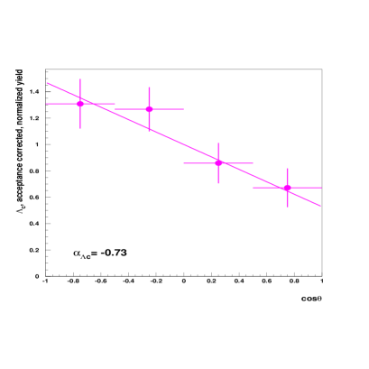
Figure 6: Visualization of the fit result for the $\Lambda_{c}^{+}\to\Lambda\pi^{+}$ sample. The way the values of the solid circles and their errors are obtained are explained in the text. The solid straight line is $1+\alpha_{\Lambda_{c}}\alpha_{\Lambda}\cos\theta_{i}$ where $\cos\theta_{i}$ is the value in the middle of the i^th bin and $\alpha_{\Lambda_{c}}\times\alpha_{\Lambda}$ is the value returned by the fit.

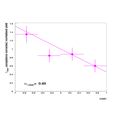
Figure 7: Visualization of the fit result for the $\overline{\Lambda}{}_{c}^{-}\to{\overline{\Lambda}}\pi^{-}$ sample. The way the values of solid circles and their errors are obtained are explained in the text. The solid straight line is $1+\alpha_{\overline{\Lambda_{c}}}\alpha_{\overline{\Lambda}}\cos\theta_{i}$ where $\cos\theta_{i}$ is the value in the middle of the i^th bin and $\alpha_{\overline{\Lambda_{c}}}\alpha_{\overline{\Lambda}}$ is the value returned by the fit.

The fit results are: $\alpha_{\Lambda_{c}}=-0.73\pm 0.21$ (with a $\chi^{2}/d.o.f.$ of 1.1) and $\alpha_{\overline{\Lambda_{c}}}=0.84\pm 0.22$ (with a $\chi^{2}/d.o.f.$ of 1.0) where the errors are statistical. These numbers lead to $\mathcal{A}=-0.07\pm 0.19$. Assuming CP invariance in this decay and taking a weighted average (after changing the sign of $\alpha_{\overline{\Lambda_{c}}}$), one obtains $\alpha_{\Lambda_{c}}=-0.79\pm 0.15$. The relative branching ratios are $\mathrm{BR}_{\Sigma^{0}}=1.14\pm 0.15$ for particles and $\mathrm{BR}_{\Sigma^{0}}=0.81\pm 0.16$ for antiparticles, leading to a weighted average of $\mathrm{BR}_{\Sigma^{0}}=0.98\pm 0.11$ The $\alpha_{\Lambda_{c}\to\Sigma^{0}\pi}$ determined by the fit were at the edge of the physical range both for the $\Lambda_{c}^{+}$ ($\alpha_{\Lambda_{c}\to\Sigma^{0}\pi}=-1$) and for the ${\overline{\Lambda}}{}_{c}^{-}$ ($\alpha_{\overline{\Lambda}_{c}\to\overline{\Sigma}^{0}\pi}$) sample, and with a very large error of 50%. In Figs. 2 and 3 the results of the fit are shown for the particle and antiparticle sample respectively, with the contribution of the $\Lambda_{c}^{+}$ signal and the $\Lambda_{c}^{+}\to\Sigma^{0}\pi^{+}$ identified. The amplitudes of the signal and of the reflection have been computed from parameters of the global fit over all four slices. A further visualization of the quality of fits are shown in Figs. 6 and 7. The number of signal events in each slice has been computed by subtracting the background and reflection from the data histograms in the region between 2.255 and 2.315 $\mathrm{GeV}/c^{2}$. The amplitudes of the background and reflection were taken from the global fit. The resulting numbers are then corrected for acceptance and normalized for comparison with the function

$$y_{i}=1+\alpha_{\Lambda_{c}}\alpha_{\Lambda}\cos\theta_{i}$$ (8)

where $y_{i}$ are the subtracted and corrected data points in the i${}^{\textrm{th}}$ $\cos\theta$ bin and $\cos\theta_{i}$ is the value of $\cos\theta$ in the middle of the i${}^{\textrm{th}}$ bin. The solid line is the function in (8) with the value of $\alpha_{\Lambda_{c}}\alpha_{\Lambda}$ returned by the fit.

4 Systematic checks

Many checks have been performed in order to assess the systematic errors on $\alpha_{\Lambda_{c}}$ and $\mathcal{A}$ .

In this analysis we assume the $\Lambda_{c}^{+}$ is produced unpolarized. We think this is a safe assumption for the FOCUS experiment. In fact if the $\Lambda_{c}^{+}$  were polarized the $\Lambda$ polarization would be larger than $\alpha_{\Lambda_{c}}$ in one hemisphere about the $\Lambda_{c}^{+}$  polarization and smaller in the other hemisphere, but the polarization averaged over all $\Lambda_{c}^{+}$ decay angles remains $\alpha_{\Lambda_{c}}$. Even a large, asymmetric error in the acceptance correction and a polarization as large as 0.5 would contribute negligibly to the systematic error. Preliminary polarization measurements [10] with this data indicate a much smaller polarization. Therefore the effect on our measurement of a possible $\Lambda_{c}^{+}$ polarization is neglible.

The fitting conditions and the cuts were changed in a reasonable manner, on the whole data set. The $\alpha_{\Lambda_{c}}$ and $\mathcal{A}$ values obtained by these variants are all a priori equally likely, therefore this uncertainty can be estimated by the r.m.s. of the measurements [11].

As explained earlier, the background shape of each $\Lambda\pi^{+}$ mass plot was fit with a second degree polynomial extracted from the wrong sign sample and only an overall scale factor was varied in the mass fit. To check how critical this assumption is, a mass fit was performed in which all twelve polynomial coefficients (three coefficients times four $\cos\theta$ bins) were fit free parameters instead of taking the shape from the wrong sign sample. The results of the fit performed in this way are $\mathcal{A}=0.06\pm 0.17$ and $\alpha_{\Lambda_{c}}=-0.84\pm 0.14$ when one assumes CP invariance. These results are in agreement with those of the standard analysis and show that the result is not sensitive to the way the background is fit. The following further systematic checks were performed:

• using a 2 $\mathrm{MeV}/c^{2}$ binning in the mass plots instead of the 5 $\mathrm{MeV}/c^{2}$ binning of the standard analysis;

• dividing the $\cos\theta$ range in 5 equally wide intervals instead of 4 intervals;

• varying the most relevant selection cuts in order to check how well the Monte Carlo reproduces the experimental apparatus, namely : variation of the $l/\sigma$ cut; variation of the cut on the transverse (with respect to the beam direction) momentum of the $\Lambda_{c}^{+}$; variation of the cut on $|\cos\omega|$; sharpening of the picon cut; variation of the cut on the proper time of the $\Lambda_{c}^{+}$ candidate; variation of the Čerenkov cut on the proton.

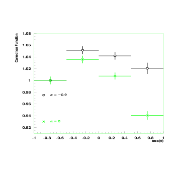
Figure 8: The correction function $\epsilon(\theta_{i},\alpha)$ corresponding to $\alpha_{\Lambda_{c}}\times\alpha_{\Lambda}=-0.9$ (circles) and to $\alpha_{\Lambda_{c}}\times\alpha_{\Lambda}=0$ (crosses) for the $\Lambda_{c}^{+}$ sample, plotted superimposed to each other. In this figure $\alpha$ means actually $\alpha_{\Lambda_{c}}\times\alpha_{\Lambda}$. All the correction functions corresponding to intermediate values, for any given $\cos\theta$ interval, lie between the values plotted on this figure.

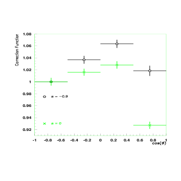
Figure 9: The correction function $\epsilon(\theta_{i},\alpha)$ corresponding to $\alpha_{\overline{\Lambda_{c}}}\times\alpha_{\overline{\Lambda}}=-0.9$ (circles) and to $\alpha_{\overline{\Lambda_{c}}}\times\alpha_{\overline{\Lambda}}=0$ (crosses) for the ${\overline{\Lambda}}{}_{c}^{-}$ sample, plotted superimposed to each other. In this figure $\alpha$ means actually $\alpha_{\overline{\Lambda_{c}}}\times\alpha_{\overline{\Lambda}}$. All the correction functions corresponding to intermediate values, for any given $\cos\theta$ interval, lie between the values plotted on this figure.

• Another check was performed to assess the possible systematic error due to errors in the correcting function $\epsilon(\theta_{i},\alpha)$ caused both by the interpolation method and by an intrinsic failure of the Monte Carlo to simulate the experimental apparatus. The correction functions that differ the most are those corresponding to the extreme values of $\alpha_{\Lambda_{c}}\,\alpha_{\Lambda}$, (or $\alpha_{\overline{\Lambda_{c}}}\,\alpha_{\overline{\Lambda}}$) namely $\alpha_{\Lambda_{c}}\,\alpha_{\Lambda}=-0.9$ and $\alpha_{\Lambda_{c}}\,\alpha_{\Lambda}=0$ (and correspondingly for the ${\overline{\Lambda}}{}_{c}^{-}$ sample) as shown by Figs. 8 and 9. The fit was performed once imposing $\alpha_{\Lambda_{c}}\,\alpha_{\Lambda}=\alpha_{\overline{\Lambda_{c}}}\,\alpha_{\overline{\Lambda}}=-0.9$ (no interpolation) and then imposing $\alpha_{\Lambda_{c}}\,\alpha_{\Lambda}=\alpha_{\overline{\Lambda_{c}}}\,\alpha_{\overline{\Lambda}}=0$. These results were taken as an indication of the magnitude of a possible systematic error.

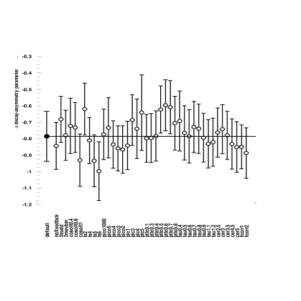
Figure 10: Summary of the systematic checks performed on $\alpha_{\Lambda_{c}}$, calculated in the hypothesis of CP conservation. The first circle on the left of plot is the result quoted in this paper.

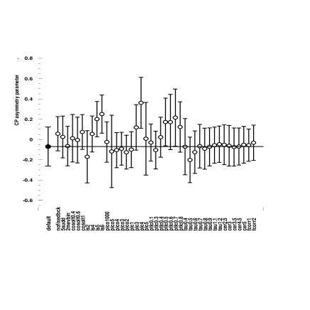
Figure 11: Summary of the systematic checks performed on $\mathcal{A}$, calculated in the hypothesis of CP conservation. The first circle on the left of plot is the result quoted in this paper.

The results for $\alpha_{\Lambda_{c}}$ and $\mathcal{A}$ for all these systematic checks are summarized in Figs. 10 and 11. As explained previously the $r.m.s.$ of all those results is taken as the estimate of the systematic error. For $\alpha_{\Lambda_{c}}$ this is $\pm 0.12$ and for $\mathcal{A}$ it is $\pm 0.13$

4.1 Check of the statistical errors returned by the fitter and possible bias

A check was performed to assure that the errors returned by the fit were realistic and to assess if there was a bias in the fitting procedure. For both the particle and the antiparticle cases, the bin contents of the four $\cos\theta$ region mass plots (Fig. 2 and 3) and the four wrong sign plots were randomly varied according to Poisson statistics 1000 times. Each set of eight ”varied” plots was analyzed with the fitting program as it were regular data and the values of $\mathcal{A}$ and $\alpha_{\Lambda_{c}}$ extracted. With this method we assessed a bias of $0.000\pm 0.005$ on $\mathcal{A}$ and we simply added $0.005$ in quadrature to the systematic error. For $\alpha_{\Lambda_{c}}$ we assessed a bias of $-0.010\pm 0.005$ and a slight underestimation of the statistical error returned by the fit (0.16 instead of 0.15). Consequently this bias was subtracted, an error of $0.005$ was added in quadrature to the systematic error and the statistical error was increased to $0.16$.

5 Final results and comparison with previous results and with the theoretical predictions

After all systematic checks, bias correction and error inflation the final results of the measurements are $\alpha_{\Lambda_{c}}=-0.78\pm 0.16\pm 0.13$ and $\mathcal{A}=-0.07\pm 0.19\pm 0.12$. Previous results obtained for $\alpha_{\Lambda_{c}}$ are listed in Table 1.

Experiment	$\alpha_{\Lambda_{c}}$
FOCUS (this result)	$-0.78\pm 0.16\pm 0.13$
CLEO II [12]	$-0.94\pm 0.21\pm 0.12$
ARGUS [13]	$-0.96\pm 0.42$
CLEO [14]	$-1.1\pm 0.4$

Table 1: Comparison of the $\alpha_{\Lambda_{c}}$ result with other experiments.

The present analysis result is a higher precision and it is in agreement with earlier results. No previous measurements for $\mathcal{A}$ have been reported.

Theoretical predictions of the two-body baryon-pseudoscalar decays of charmed baryons have been made by a number of authors in the past.

Paper	$\alpha_{\Lambda_{c}}$
Ivanov et al. [15](1998)	$-0.95$
Zenczykowski [16](1994)	$-0.99$
Zenczykowski [17](1994)	$-0.86$
Uppal et al. [18](1994)	$-0.85$
Cheng and Tseng [19](1993)	$-0.95$
Cheng and Tseng [20](1992)	$-0.96$
Xu and Kamal [21](1992)	$-0.67$
Körner and Kramer [22](1992)	$-0.70$

Table 2: Summary of the most recent theoretical predictions on $\alpha_{\Lambda_{c}}$ (under the CP conservation hypothesis)

They predict the parity conserving amplitude $A_{+}$ and parity violating amplitude $A_{-}$ of Eqn. (4) from which $\alpha_{\Lambda_{c}}$ and the decay rate can be derived. The most recent predictions are listed in Table 2. All predictions are in agreement within errors with the FOCUS experimental result.

6 Conclusions

Using data from the FOCUS (E831) experiment at Fermilab, we have studied the decay mode $\Lambda_{c}^{+}\to\Lambda\pi^{+}$ and measured the asymmetry parameter $\alpha_{\Lambda_{c}}$ (under the CP conservation hypothesis) and the CP parameter $\mathcal{A}$ . Our result for $\alpha_{\Lambda_{c}}$ is consistent with previous measurements and is more accurate. Our result for $\mathcal{A}$ is the first measurement of this quantity and is consistent with zero.

We wish to acknowledge the assistance of the staffs of Fermi National Accelerator Laboratory, the INFN of Italy, and the physics departments of the collaborating institutions. This research was supported in part by the U. S. National Science Foundation, the U. S. Department of Energy, the Italian Istituto Nazionale di Fisica Nucleare and Ministero della Istruzione Università e Ricerca, the Brazilian Conselho Nacional de Desenvolvimento Científico e Tecnológico, CONACyT-México, and the Korea Research Foundation of the Korean Ministry of Education.

Figure 1: $\Lambda\pi$ effective mass after the selection. a) total sample; b) $\Lambda\pi^{+}$ sample; c) $\overline{\Lambda}\pi^{-}$ sample.

Figure 2: $\Lambda\pi^{+}$ effective mass for the $\Lambda_{c}^{+}$ subsample in each $\cos\theta$ bin: a) $-1<\cos\theta<-0.5$; b) $-0.5<\cos\theta<0$; c) $0<\cos\theta<0.5$; d) $0.5<\cos\theta<1$. The results of the analysis fit (solid line) are shown superimposed on the plots. The $\Lambda_{c}^{+}\to\Lambda\pi^{+}$ contribution to the fit is shown by the solid histogram, the $\Lambda_{c}^{+}\to\Sigma^{0}\pi^{+}$ contribution by the hatched histogram.

Figure 3: $\overline{\Lambda}\pi^{-}$ effective mass for the ${\overline{\Lambda}}{}_{c}^{-}$ subsample in each $\cos\theta$ bin: a) $-1<\cos\theta<-0.5$; b) $-0.5<\cos\theta<0$; c) $0<\cos\theta<0.5$; d) $0.5<\cos\theta<1$. The results of the analysis fit (solid line) are shown superimposed on the plots. The $\overline{\Lambda}{}_{c}^{-}\to{\overline{\Lambda}}\pi^{-}$ contribution to the fit is shown by the solid histogram, the $\overline{\Lambda}{}_{c}^{-}\to\overline{\Sigma}^{0}\pi^{-}$ contribution by the hatched histogram.

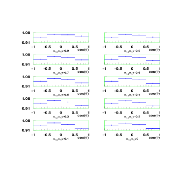
Figure 4: Correction function $\epsilon(\theta_{i},\alpha)$ calculated from Monte Carlo, for the $\Lambda_{c}^{+}$ sample, at ten values of $\alpha_{\Lambda_{c}}\times\alpha_{\Lambda}$, spanning the range from $-0.9$ to 0. All correction functions are normalized such that they are 1 in the first $\cos\theta$ bin. Note that an overall normalizing factor can be chosen for the correction functions without changing the result of the fit.

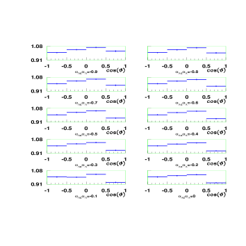
Figure 5: Correction function $\epsilon(\theta_{i},\alpha)$ calculated from Monte Carlo, for the ${\overline{\Lambda}}{}_{c}^{-}$ sample, at ten values of $\alpha_{\overline{\Lambda_{c}}}\times\alpha_{{\overline{\Lambda}}}$, spanning the range from $-0.9$ to 0. All correction functions are normalized such that they are 1 in the first $\cos\theta$ bin.

References

- [1] G. Källén, “Elementary Particle Physics,” Addison-Wesley Publishing Company, Inc., 1964.
- [2] S. Eidelman et al., (Particle Data Group), Phys. Lett. B 592 (2004), 1.
- [3] E687 Collaboration, P.L. Frabetti et al., Nucl. Instrum. Meth. A 320 (1992) 519.
- [4] E687 Collaboration, P.L. Frabetti et al., Nucl. Instrum. Meth. A 329 (1993) 62.
- [5] FOCUS Collaboration, J.M. Link et al., Nucl. Instrum. Meth. A 516(2004) 364.
- [6] FOCUS Collaboration, J.M. Link at al., Nucl. Instrum. Meth. A 484 (2002) 174.
- [7] FOCUS Collaboration, J.M. Link et al., Nucl. Instrum. Meth. A 484 (2002) 270.
- [8] R. Gatto, Phys. Rev. 109 (1957) 610.
- [9] J. Dreitlein and H. Primakoff, Phys. Rev. 125 (1962) 1671.
- [10] C. Castromonte, thesis: “Study of the polarization of the baryon in photon-nucleon interactions,” Centro Brasileiro de Pesquisas Fisicas - CBPF, Rio de Janeiro, December 2004.
- [11] FOCUS Collaboration, J.M. Link et al., Phys. Lett. B 555 (2003) 167.
-
[12]
CLEO II Collaboration,
M. Bishai et al., Phys. Lett. B 350 (1995) 256.
Note that for the error on the CLEO II result, we followed the PDG 2004 point of view explained by the following quotation from them: [the CLEO II paper] “actually gives , chopping the errors at the physical limit -1.0. However, for , some experiments should get unphysical values () and for averaging with other measurements such values (or errors that extend below ) should not be chopped” - [13] ARGUS Collaboration, H. Albrecht et al., Phys. Lett. B 274 (1992) 239.
- [14] CLEO Collaboration, P. Avery et al., Phys. Rev. Lett. 65 (1990) 2842.
- [15] M.A. Ivanov, J.G. Körner, V.E. Lyubovitskij, and A.G. Rusetsky, Phys. Rev. D 57 (1998) 5632.
- [16] P. Zenczykowski, Phys. Rev. D 50 (1994) 5787.
- [17] P. Zenczykowski, Phys. Rev. D 50 (1994) 402.
- [18] T. Uppal, R.C. Verma, and M.P. Khanna, Phys. Rev. D 49 (1994) 3417.
- [19] H. Cheng and B. Tseng, Phys. Rev. D 48 (1993) 4188.
- [20] H. Cheng and B. Tseng, Phys. Rev. D 46 (1992) 1042.
- [21] Q.P. Xu and A.N. Kamal, Phys. Rev. D 46 (1992) 270.
- [22] J.G. Körner and M. Kramer, Z. Phys. C 55 (1992) 659.