Bose-Einstein Correlations in e⁺e^- Annihilation and e⁺e${}^{-}\rightarrow\mathrm{W}^{+}\mathrm{W}^{-}$

Abstract

Results on Bose-Einstein correlations in $\mathrm{e}^{+}\mathrm{e}^{-}\rightarrow\mathrm{hadrons}$ are reviewed.

1 Introduction

Bose-Einstein correlations (BEC) are those correlations which arise as a consequence of Bose symmetry, which leads to an enhancement of the production of identical particles close together in phase space. In this talk I will review some of the results on BEC from $\mathrm{e^{+}}$$\mathrm{e^{-}}$ interactions.

To study correlations among $q$ particles, we begin with the inclusive $q$-particle density,

$$\rho_{q}(p_{1},...,p_{q})=\frac{1}{\sigma_{\mathrm{tot}}}\frac{\mathrm{d}^{q}\sigma_{q}(p_{1},...,p_{q})}{\mathrm{d}{p_{1}}...\mathrm{d}p_{q}}$$ (1)

where $\sigma_{q}$ is the inclusive $q$-particle cross section. These densities are normalized such that

$$\int\rho_{1}(p)\,{{\mathrm{d}}p} = \langle n\rangle$$ (2)

$$\int\rho_{2}(p_{1},p_{2})\,{{\mathrm{d}}p_{1}}\,{{\mathrm{d}}p_{2}} = \langle n(n-1)\rangle$$ (3)

$$\int\rho_{2}(p_{1},p_{2},p_{3})\,{{\mathrm{d}}p_{1}}\,{{\mathrm{d}}p_{2}}\,{{\mathrm{d}}p_{3}} = \langle n(n-1)(n-2)\rangle\ ,$$ (4)

etc., and are related to the factorial cumulants, $C$, by

$$\rho_{1}(p_{1}) = C_{1}(p_{1})$$ (5)

$$\rho_{2}(p_{1},p_{2}) = C_{1}(p_{1})C_{1}(p_{2})+C_{2}(p_{1},p_{2})$$ (6)

$$\rho_{3}(p_{1},p_{2},p_{3})) = C_{1}(p_{1})C_{1}(p_{2})C_{1}(p_{3})$$ (7)

$$+ \sum_{\textrm{3\ perms}}C_{1}(p_{1})C_{2}(p_{2},p_{3})$$

$$+ C_{3}(p_{1},p_{2},p_{3})\ .$$

The $q$-particle correlations are then measured by $\rho_{q}-\prod_{i=1}^{q}C_{1}(p_{i}1)$. For $q>2$, the correlations are a sum of “trivial”, i.e., arising trivially from correlations of smaller $q$, and “genuine” correlations. For example, for $q=3$ the trivial correlations are given by $\sum_{\textrm{3\ perms}}C_{1}(p_{1})C_{2}(p_{2},p_{3})$ and the genuine correlations by $C_{3}$.

It is convenient to normalize $\rho$ and $C$:

$$\mathsf{R}_{q} = \frac{\rho_{q}}{\prod_{i=1}^{q}\rho_{1}(p_{i})}$$ (8)

$${K}_{q} = \frac{C_{q}}{\prod_{i=1}^{q}\rho_{1}(p_{i})}\ .$$ (9)

In order to study BEC, and not other correlations, one usually studies the ratio of the above-defined $\mathsf{R_{q}}$ to the $\mathsf{R_{q}}$ that one expects in the absence of BEC. This is equivalent to replacing the product of single-particle densities in (8) by the $q$-particle density expected when BEC is absent, $\rho_{0q}$, giving:

$$R_{q}=\frac{\rho_{q}}{\rho_{0q}}\ .$$ (10)

This ratio is usually regarded as a function of $Q$, where $Q^{2}=M_{q}^{2}-(qm)^{2}$ with $M_{q}$ the mass of the $q$ particles and $m$ the mass of each particle. If the particles have identical 4-momenta. $Q=0$. For 2 particles, $Q^{2}$ is simply the 4-momentum difference. Thus, e.g., 2-particle BEC are studied using

$$R_{2}(Q)=\frac{\rho(Q)}{\rho_{0}(Q)}\ ,$$ (11)

where the subscript $q$ has been suppressed.

It can be shown in a variety of ways that $R_{q}$ is related to the spatial distribution of the particle production Goldhaber et al. (1960); Boal et al. (1990). For example, assuming incoherent particle production and a spatial source density of pion emitters, $S(x)$, leads to

$$R_{2}(Q)=1+\left|{G(q)}\right|^{2}\ .$$ (12)

where $G(Q)\!=\!\int\!\,{{\mathrm{d}}x}\,e^{\imath Qx}S(x)$ is the Fourier transform of $S(x)$. Assuming $S(x)$ is a Gaussian with radius $r$ results in

$$R_{2}(Q)=1+e^{-Q^{2}r^{2}}\ .$$ (13)

Customarily, an additional parameter, $\lambda$, is introduced in (13):

$$R_{2}(Q)=1+\lambda e^{-Q^{2}r^{2}}\ .$$ (14)

This parameter is meant to account for several effects:

• partial coherence. Completely coherent particle production would imply $\lambda=0$.

• multiple sources.

• particle purity, e.g., experimental difficulty in distinguishing pions from kaons.

The assumption of a spherical (radius $r$) Gaussian distribution of particle emitters seems unlikely in $\mathrm{e^{+}}$$\mathrm{e^{-}}$ annihilation, where there is a definite jet structure. However, we must keep in mind that the BEC only occur among particles produced close to each other in phase space. In a two-jet event, a particle produced in the core of one jet would not be “close” to a particle produced in the core of the other jet. The volume in which hadronization occurs may thus be larger than a sphere of radius $r$ and is not necessarily spherical.

Furthermore, no time dependence has been considered, i.e., the source has been assumed to be static, which is certainly wrong.

A number of other parametrizations have been considered in the literature. Nevertheless, in spite of the above-noted limitations, this Gaussian parametrization (14) is the one most frequently used by experimentalists. When this Gaussian parametrization does not fit well, an expansion about the Gaussian (Edgeworth expansion Edgeworth (1905)) can be used instead. Keeping only the lowest-order non-Gaussian term, $\exp(-Q^{2}r^{2})$ becomes $\exp(-Q^{2}r^{2})\cdot\left[1+\frac{\kappa}{3!}H_{3}(Qr)\right]$, where $H_{3}$ is the third-order Hermite polynomial.

In the interest of comparison of as much data as possible, I shall only consider results using the Gaussian or Edgeworth parametrizations here.

2 Experimental Difficulties

There are a number of experimental problems which affect the results on BEC and their interpretation.

Particle purity influences the value of $\lambda$. In studying BEC of pions, it is often assumed that all particles are pions, which is not true. For example, in $\mathrm{Z}$-boson decays approximately 15% of the particles are not pions. This lowers the observed value of $\lambda$. The value of $r$ for BEC involving a particle from a long-lived resonance and one produced directly, or involving particles from different long-lived resonances, will be larger than for two particles produced directly. Consequently, the resulting enhancement at small $Q$ in $R_{2}(Q)$ will be narrower, possibly narrower than the experimental resolution, which in turn reduces the observed value of $\lambda$. On the other hand, the effect of short-lived resonances is to increase the observed value of $r$, since it takes into account, in some average way, the distance the resonance travels before decaying. In $\mathrm{Z}$-boson decays only about 16% of charged pions are produced directly, while 62% come from short-lived ($\Gamma>6.7\,\mathrm{M}{\mathrm{e\kern-0.80002ptV}}$) and 22% from long-lived resonances. Particles from weak decays are produced far away from the others, so that there are no BEC between pions from the weak decay and the rest. This results in a smaller value of $\lambda$. About 20% of $\mathrm{Z}$-bosons decay to $\mathrm{b}$$\bar{\mathrm{b}}$. Not only the values of $\lambda$ and $r$ may be influenced by resonances, but also the shape of $R_{2}$. One can attempt to correct for all of these effects, typically by using a Monte Carlo model. However, the correctness of the model is open to question.

A second problem is the choice of the so-called reference sample, i.e., the sample for which $\rho_{0}$ is the density. Since it is impossible to turn off Bose statistics, this sample does not exist. It must be created artificially. Common choices are unlike-sign pairs, Monte Carlo models, and mixed events. When studying BEC in like-sign pion pairs one can use unlike-sign pion pairs to form the reference sample. The main problem is that the unlike-sign pairs have resonances which the like-sign pairs do not. This is illustrated in Fig. 1a, where $R_{2}$ calculated using an unlike-sign pair reference sample is shown for $\mathrm{Z}$-decay data and for Monte Carlo. Structure in $R_{2}$ due to resonances in the reference sample is clearly seen. One might think of correcting for this using Monte Carlo, but this will only work if the resonances are well-described in the Monte Carlo. This is clearly not the case here, as is seen in Fig. 1b. The solution adopted is to exclude the affected regions from the fit of (14) to the data. These regions, indicated in Fig. 1, cover large ranges in $Q$, and one must ask whether larger, or additional, excluded regions are needed.

Figure 1: (a) $R_{2}$ (here called $C$) for $\mathrm{Z}$-decay data and Monte Carlo; (b) the ratio of $R_{2}$ of the data to that of the Monte Carlo.

Using Monte Carlo as the reference sample avoids the different resonances of like- and unlike-sign pairs, but is still not completely free of resonance problems. Reflections of unlike-sign resonances and multi-body resonance decays, e.g., $\mathrm{\eta^{\prime}(958)}\rightarrow\mathrm{\pi^{+}}\mathrm{\pi^{-}}\mathrm{\eta}\rightarrow\mathrm{\pi^{+}}\mathrm{\pi^{-}}\mathrm{\pi^{+}}\mathrm{\pi^{-}}\mathrm{\pi^{0}}$, still affect $\rho_{0}$. But these effects are small compared to the use of unlike-sign pairs as the reference sample. Another problem with using a Monte Carlo reference sample is the description of fragmentation. In a Monte Carlo model, fragmentation is controled by some parameters whose values are chosen to give a good description of the data. However, the data contain BEC. If the Monte Carlo does not include a description of BEC, the fragmentation parameters will be chosen so as to describe (in so far as is possible) BEC as well as the fragmentation itself. The reference sample will then have some enhancement in $\rho$ at small $Q$, and its use as reference sample will result in a smaller value of $\lambda$. The value of $r$ may also be affected. On the other hand, a BEC model can be included in the Monte Carlo and the fragmentation parameters determined. Then the BEC model can be turned off to construct the reference sample. How good this reference sample is depends on how well the BEC were modeled. To model them well would require not only knowing how to correctly model BEC but also knowing the results of the BEC analysis before doing it.

Event mixing involves taking pairs of particles from different events. For each real event, a similar event is constructed by replacing each particle by a particle from a different event. This procedure, of course, removes all correlations, not just BEC. Therefore, care should be taken in choosing the particles in order to have a reference sample similar to the real sample in characteristics such as jet structure. In this way some kinematic correlations can be preserved. Other correlations can be reinstated using the results of applying the same mixing procedure to Monte Carlo, i.e., by using the double ratio $R_{2}/R_{2}^{\mathrm{MC}}$ instead of $R_{2}$ itself. Thus this method is also not entirely free of Monte Carlo uncertainties. For 2-jet events one can mix hemispheres instead of events. In this approach the reference sample is constructed by pairing a particle from one hemisphere with a particle from the other hemisphere which has been reflected through the origin.

A third problem is final-state interactions, both Coulomb and strong. Identical charged particles will be repulsed by the Coulomb interaction, decreasing the observed value of $\lambda$ and increasing the observed value of $r$. The most common way to take this into account is to multiply $R_{q}$ by a correction factor before fitting (14) to the data. The correction factor most commonly used is the so-called Gamow factor Gyulassy et al. (1979), which is the modulus square of the non-relativistic Coulomb wave function at the origin. For 2-particle BEC, given the resolution of the lep experiments, the correction is only a few per cent in the lowest $Q$ bin (twice that if an unlike-sign reference sample is used), and is therefore frequently ignored. However for 3-particle BEC it is of the order of 10%.

A different approach is to incorporate both the Coulomb and the $S=0$ $\pi\pi$ phase shifts into the wave function and derive a corrected formula for $R_{2}$. An example of this approach is shown in Fig. 2 Osada et al. (1996). Significant differences are found in the values of $\lambda$ and $r$, which are listed in Table 1. However, such sophisticated approaches have not been used by any of the experimental groups.

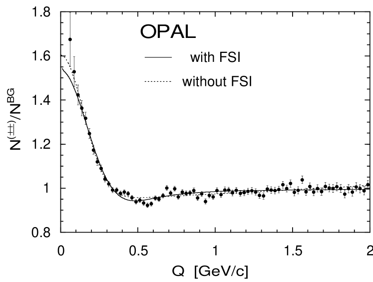
Figure 2: Fits with and without FSI (Coulomb and $S=0$ $\pi\pi$ phase shifts) to opal Z-decay data Osada et al. (1996).

FSI	$\lambda$	$r$ (fm)
with	$1.04\pm 0.03$	$1.09\pm 0.04$
without	$0.71\pm 0.04$	$1.34\pm 0.04$

Table 1: Results of fits Osada et al. (1996) with and without FSI (Coulomb and $S=0$ $\pi\pi$ phase shifts) to opal Z-decay data.

Finally, there is the effect of long-range correlations not adequately taken into account by the reference sample. As observed, e.g., in Fig. 2, $R_{2}$ is not constant at large $Q$. To account for this in fitting the data, the right hand side of (14) is multiplied by an appropriate factor, usually a linear dependence on $Q$,

$$R_{2}(Q)=\gamma\left(1+\lambda e^{-Q^{2}r^{2}}\right)\left(\vphantom{e^{Q^{2}}}1+\delta Q\right)\ ,$$ (15)

although a quadratic dependence may also be used if necessary, and the normalization, $\gamma$, is usually left as a free parameter.

3 Experimental Results

Now let us turn to a comparison of results from various $\mathrm{e^{+}}$$\mathrm{e^{-}}$ experiments.

3.1 2-particle BEC

Dependence on the reference sample

The values of $\lambda$ and $r$ found using identical charged-pion pairs from hadronic $\mathrm{Z}$ decays in the lep experiments, aleph ALEPH Collab. et al. (1992, 2004), delphi DELPHI Collab. et al. (1992), l3 L3 Collab. et al. (2002a) and opal OPAL Collab. et al. (1991, 1996a, 2000) are displayed in Fig. 3.

Although these points are all supposed to be measurements of the same quantitities and are all determined by fitting the Gaussian parametrization to $R_{2}$, there is little agreement among the points. Clearly there must be large systematic uncertainties not accounted for. Indeed, most of the points have only statistical error bars. However, some have error bars including also systematic uncertainties. But these are clearly insufficient.

Solid points are corrected for pion purity, while open points are not. It is apparent that this correction increases the value of $\lambda$ but has little effect on the value of $r$.

All of the results with $r>0.1$ fm were obtained using an unlike-sign reference sample, while all of those with smaller $r$ were obtained with a mixed reference sample. It is clear that the choice of reference sample has a large effect on the values of the parameters. In comparing the results of different experiments, we must therefore be sure that the reference samples used are comparable.

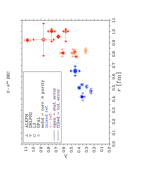
Figure 3: $\lambda$ and $r$ at $\sqrt{s}=M_{\mathrm{Z}}$ found in the lep experiments ALEPH Collab. et al. (1992, 2004); DELPHI Collab. et al. (1992); L3 Collab. et al. (2002a); OPAL Collab. et al. (1991, 1996a, 2000). Open arrow-heads at the end of error bars indicate that the uncertainties are statistical only, filled arrow-heads that the uncertainties are combined statistical and systematic.

Dependence on the center-of-mass energy

The values of $r$ found using identical charged-pion pairs in $\mathrm{e^{+}}$$\mathrm{e^{-}}$ annihilation is shown versus the center of mass energy, $\sqrt{s}$, in Fig. 4. Keeping in mind that we should compare only results using the same reference sample, we conclude that there is no evidence for a $\sqrt{s}$ dependence.

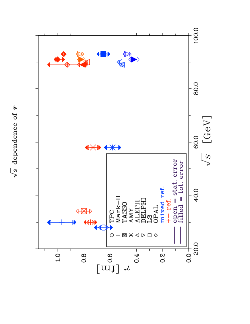
Figure 4: $\sqrt{s}$ dependence of $r$ Aihara et al. (1985); Juricic et al. (1989); TASSO Collab. et al. (1986); AMY Collab. et al. (1995); ALEPH Collab. et al. (1992, 2004); DELPHI Collab. et al. (1992); L3 Collab. et al. (2002a); OPAL Collab. et al. (1991, 1996a, 2000). For clarity some points are shifted slightly in $\sqrt{s}$. Open arrow-heads at the end of error bars indicate that the uncertainties are statistical only, filled arrow-heads that the uncertainties are combined statistical and systematic.

Dependence on the particle mass

It has been suggested, on several grounds Alexander (2003), that $r$ should depend on the mass of the particle as $r\propto 1/\sqrt{m}$. Results from lep experiments on $r$ from 2-particle BEC for charged pions and for kaons, as well as the corresponding Fermi-Dirac correlations for protons and lambdas, are shown in Fig. 5. Again, restricting our comparison to results which have used the same type of reference sample (in this case mixed), we see no evidence for a $1/\sqrt{m}$ dependence. Rather, the data suggest one value of $r$ for mesons and a smaller value for baryons. The value for baryons, about 0.1 fm, seems very small; if true it is telling us something unexpected about the mechanism of baryon production.

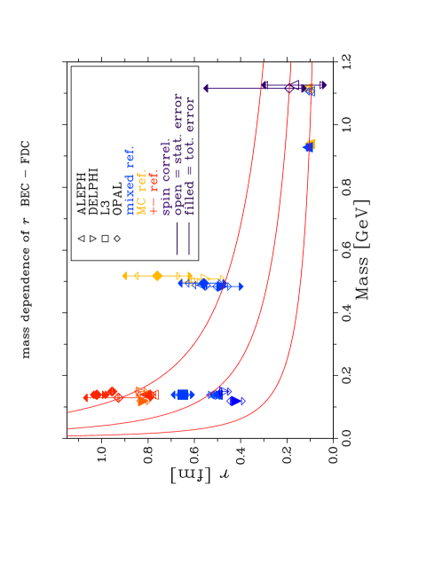
Figure 5: Dependence of $r$ on the mass of the particle as determined at $\sqrt{s}=M_{\mathrm{Z}}$ from 2-particle BEC for charged pions ALEPH Collab. et al. (1992, 2004); DELPHI Collab. et al. (1992); L3 Collab. et al. (2002a); OPAL Collab. et al. (1991, 1996a, 2000), charged kaons DELPHI Collab. et al. (1996); OPAL Collab. et al. (2001) and neutral kaons ALEPH Collab. et al. (2005a); DELPHI Collab. et al. (1996); OPAL Collab. et al. (1995) and from Fermi-Dirac correlations for protons ALEPH Collab. et al. (2005a) and lambdas ALEPH Collab. et al. (2000a); OPAL Collab. et al. (1996b). Open arrow-heads at the end of error bars indicate that the uncertainties are statistical only, filled arrow-heads that the uncertainties are combined statistical and systematic. The curves illustrate a $1/\sqrt{m}$ dependence.

Dependence on the particle multiplicity

The values of $\lambda$ and $r$ from charged-pion 2-particle BEC depend on the charged particle multiplicity, $n_{\mathrm{ch}}$, of the events. As seen in Fig. 6, $\lambda$ decreases with $n_{\mathrm{ch}}$ while $r$ increases. However, a similar dependence is also seen on the number of jets. When 2-jet events are selected, little, if any, dependence on $n_{\mathrm{ch}}$ remains. For 3-jet events, $r$ seems independent of $n_{\mathrm{ch}}$, although $\lambda$ does decrease with $n_{\mathrm{ch}}$. Thus, the dependence of $\lambda$ and $r$ on $n_{\mathrm{ch}}$ seems to be largely due to a dependence on the number of jets.

Figure 6: Dependence of $\lambda$ and $r$ from charged-pion 2-particle BEC on the charged particle multiplicity, $n_{\mathrm{ch}}$, and on the number of jets OPAL Collab. et al. (1996a).

Elongation of the source

The Gaussian parametrization (14) assumes a spherical source. Given the jet structure of $\mathrm{e^{+}}$$\mathrm{e^{-}}$ events, one might expect a more ellipsoidal shape. To investigate this, the parametrization is generalized to allow different radii for the direction along and perpendicular to the jet axis. The analysis is perfomed in the longitudinal center of mass system (LCMS), which is defined as follows: The pion pair is boosted along the jet-axis (taken, e.g., as the thrust axis), to a frame where the sum of the longitudinal momenta of the two pions is zero. The transverse axes, called “out” and “side” are defined such that the out direction is along the vector sum of the two momenta, $\vec{p_{1}}+\vec{p_{2}}$, and the side direction completes the Cartesian coordinate frame. This is illustrated in Fig. 7.

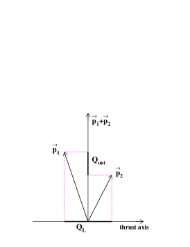
$p_{\mathrm{L1}}=-p_{\mathrm{L2}}$

$\vec{p}_{1}+\vec{p}_{2}$ defines ‘out’ axis

$Q_{\mathrm{side}}\perp(Q_{\mathrm{L}},Q_{\mathrm{out}})$

Figure 7: The definition of the longitudinal center of mass system (LCMS).

In the LCMS,

$$Q^{2} = Q_{\mathrm{L}}^{2}+Q_{\mathrm{side}}^{2}+Q_{\mathrm{out}}^{2}-(\Delta E)^{2}$$ (16)

$$= Q_{\mathrm{L}}^{2}+Q_{\mathrm{side}}^{2}+Q_{\mathrm{out}}^{2}(1-\beta^{2}),\quad\mathrm{where}\quad\beta\equiv\frac{p_{\mathrm{out}\,1}+p_{\mathrm{out}\,2}}{E_{1}+E_{2}}\ .$$

The advantage of the LCMS is immediately apparent: The energy difference, and therefore the difference in emission time of the pions, couples only to the out component, $Q_{\mathrm{out}}$. Thus $Q_{\mathrm{L}}$ and $Q_{\mathrm{side}}$ reflect only spatial dimensions of the source, while $Q_{\mathrm{out}}$ reflects a mixture of spatial and temporal dimensions. The Gaussian parametrization (15) becomes

$$R_{2}(Q_{\mathrm{L}},Q_{\mathrm{side}},Q_{\mathrm{out}})=\gamma\left(1+\lambda G\right)\left(1+\delta Q_{\mathrm{L}}+\epsilon Q_{\mathrm{out}}+\xi Q_{\mathrm{side}}\right)\ .$$ (17)

Assuming an azimuthally symmetric Gaussian shape, there is only one non-zero off-diagonal term, and $G$ is given by

$$G=\exp\left(-r^{2}_{\mathrm{L}}{Q_{\mathrm{L}}^{2}}-r^{2}_{\mathrm{out}}{Q_{\mathrm{out}}^{2}}-r^{2}_{\mathrm{side}}{Q_{\mathrm{side}}^{2}}+2\rho_{\mathrm{L,out}}{r_{\mathrm{L}}r_{\mathrm{out}}}{Q_{\mathrm{L}}Q_{\mathrm{out}}}\right)\ .$$ (18)

Such an analysis has been performed by l3 L3 Collab. et al. (1999) and opal OPAL Collab. et al. (2000). In fact, $\rho_{\mathrm{L,out}}$ turns out consistent with zero, and is then fixed to zero in the fits. Two-dimensional LCMS analyses have been performed by aleph ALEPH Collab. et al. (2004) and delphi DELPHI Collab. et al. (2000), in which the out and side components are replaced by a transverse one, $Q^{2}_{\mathrm{t}}=Q_{\mathrm{out}}^{2}+Q_{\mathrm{side}}^{2}$. However, the interpretation of the corresponding parameter, $r_{\mathrm{t}}$, as a transverse radius is not unambiguous, since it includes the effect of the difference in time of emission. Both l3 and aleph fit not only (17), but a similar expression where $G$ is replaced by a lowest-order Edgeworth expansion, which gives a better fit (e.g., in l3, a confidence level of 30% compared with 3% for the Gaussian fit). The ratio of transverse to longitudinal radii found in the four experiments are shown in Table 2. The longitudal radius is clearly about 20% larger than the transverse radius.

Experiment	Data	Reference	Gauss /	2-D			3-D
		sample	Edgeworth	$r_{\mathrm{t}}/r_{\mathrm{L}}$			$r_{\mathrm{side}}/r_{\mathrm{L}}$
delphi	2-jet	mixed	Gauss	0.62$\pm$	0.02 $\pm$	0.05	—
aleph	2-jet	mixed	Gauss	0.61$\pm$	0.01 $\pm$	0.??	—
	2-jet	+ –	Gauss	0.91$\pm$	0.02 $\pm$	0.??	—
	2-jet	mixed	Edgeworth	0.68$\pm$	0.01 $\pm$	0.??	—
	2-jet	+ –	Edgeworth	0.84$\pm$	0.02 $\pm$	0.??	—
opal	2-jet	+ –	Gauss	—			0.82$\pm$	0.02 $\pm$	${{}^{0.01}_{0.05}}$
l3	all	mixed	Gauss	—			0.80$\pm$	0.02 $\pm$	${{}^{0.03}_{0.18}}$
	all	mixed	Edgeworth	—			0.81$\pm$	0.02 $\pm$	${{}^{0.03}_{0.19}}$

Table 2: Ratio of transverse or side radius to longitudinal radius from charged-pion 2-particle BEC analyses of retail organisation

In Fig. 8 we see that the amount of this elongation increases when narrower 2-jet events are selected.

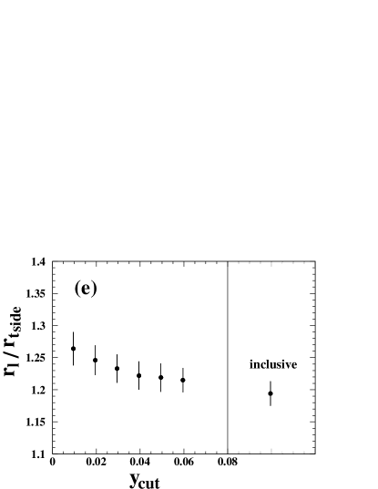
Figure 8: The ratio of $r_{\mathrm{L}}$ to $r_{\mathrm{side}}$ for 2-jet events as function of the jet resolution parameter, $y_{\mathrm{cut}}$.

It should also be mentioned that zeus ZEUS Collab. et al. (2004) performed a similar 2-dimensional analysis in deep inelastic ep interactions. The ratio $r_{\mathrm{t}}/r_{\mathrm{L}}$ found, similar to that found by delphi and aleph, is independent of the virtuality of the exchanged photon.

$\mathrm{\pi^{0}}$$\mathrm{\pi^{0}}$

In hadronization models with local charge conservation, e.g., string models, neutral pions can be produced closer together than identical charged pions. One could expect this to be reflected in a smaller BEC radius for $\mathrm{\pi^{0}}$$\mathrm{\pi^{0}}$ than for $\pi^{\pm}\pi^{\pm}$. Only two $\mathrm{e^{+}}$$\mathrm{e^{-}}$ experiments have attempted a BEC analysis of $\mathrm{\pi^{0}}$$\mathrm{\pi^{0}}$, l3 L3 Collab. et al. (2002b) and opal OPAL Collab. et al. (2003). The experimental selections used in the two analyses are quite different, dictated as they are by the characteristics of the different detectors. While l3 requires the energy of the pions to be less than 6 $\mathrm{G}{\mathrm{e\kern-0.80002ptV}}$, opal demands the $\mathrm{\pi^{0}}$ momenta to be greater than 1 $\mathrm{G}{\mathrm{e\kern-0.80002ptV}}$. Further, opal uses only 2-jet events, defined as having thrust larger than 0.9.

The $R_{2}$ distributions and fits are shown in Figs. 9 and 10, respectively. In order to make a comparison with charged pions, l3 also analyzes $\pi^{\pm}\pi^{\pm}$ with a selection similar to its $\mathrm{\pi^{0}}$ selection. The resulting $R_{2}$ is also shown in Fig. 9. The results of fits to these distributions, as well as two other $\pi^{\pm}\pi^{\pm}$ results are listed in Table 3.

Comparison of the l3 values of $r$ for $\mathrm{\pi^{0}}$$\mathrm{\pi^{0}}$ and $\pi^{\pm}\pi^{\pm}$ with the same selection indicates that the radius is smaller in the $\mathrm{\pi^{0}}$$\mathrm{\pi^{0}}$ case, but the significance is only about 1.5 standard deviations. $\lambda$ is also smaller in the $\mathrm{\pi^{0}}$$\mathrm{\pi^{0}}$ case, with similar significance.

For opal, the comparison is more difficult to make, since opal’s charged-pi results use a different reference sample and different selection. Other experiments have found that the ratio of $r$ using a mixed reference sample to that using unlike-sign is about 0.68 (aleph ALEPH Collab. et al. (2004)) or 0.56 (delphi DELPHI Collab. et al. (1992)). Applying such a factor would lower the opal value to about 0.62, which agrees well with the opal result for $\mathrm{\pi^{0}}$$\mathrm{\pi^{0}}$. However, it is not clear what the effect of the 2-jet and $\mathrm{\pi^{0}}$-momentum cuts is. In the l3 case, requiring the pions to have $E<6\,\mathrm{G}{\mathrm{e\kern-0.80002ptV}}$ and using a Monte Carlo reference sample rather than a mixed one decreased $r$ by about 30%. It is therefore conceivable that the opal requirement of $p>1\,\mathrm{G}{\mathrm{e\kern-0.80002ptV}}$ would increase $r$, in which case $r$ for $\mathrm{\pi^{0}}$$\mathrm{\pi^{0}}$ would be smaller than for $\pi^{\pm}\pi^{\pm}$.

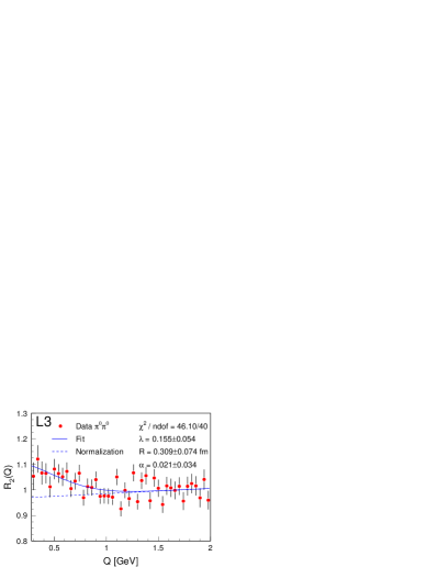
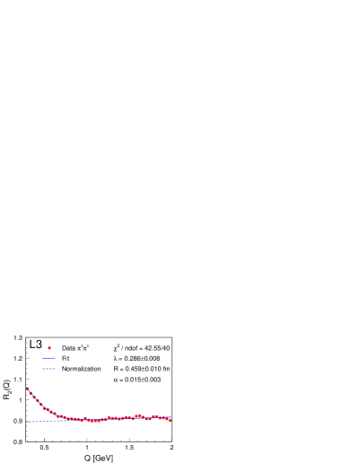
Figure 9: $R_{2}$ distribution for $\mathrm{\pi^{0}}$$\mathrm{\pi^{0}}$ and for $\pi^{\pm}\pi^{\pm}$ L3 Collab. et al. (2002b).

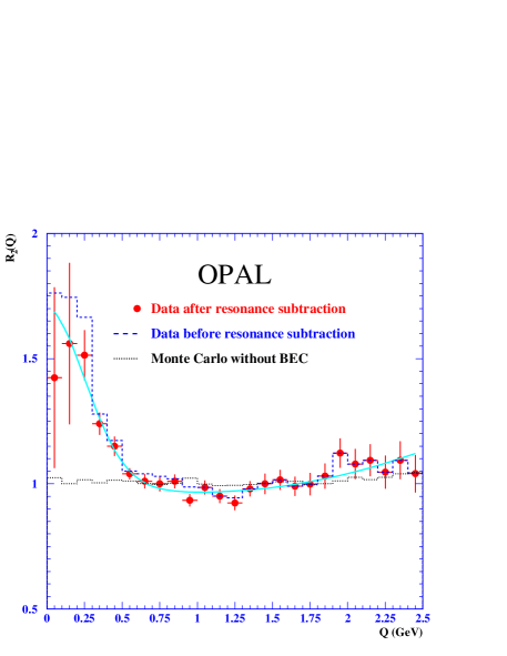
Figure 10: $R_{2}$ distribution for $\mathrm{\pi^{0}}$$\mathrm{\pi^{0}}$ OPAL Collab. et al. (2003).

			Reference
	Experiment	Selection	sample	$r$ (fm)	$\lambda$
$\mathrm{\pi^{0}}\mathrm{\pi^{0}}$	l3	$E_{\mathrm{\pi}}<6\,\mathrm{G}{\mathrm{e\kern-0.80002ptV}}$	MC	$0.31\pm 0.10$	$0.16\pm 0.09$
	opal	$p_{\mathrm{\pi}}>1\,\mathrm{G}{\mathrm{e\kern-0.80002ptV}}$, 2-jet	mix	$0.59\pm 0.09$	$0.55\pm 0.14$
$\pi^{\pm}\pi^{\pm}$	l3	$E_{\mathrm{\pi}}<6\,\mathrm{G}{\mathrm{e\kern-0.80002ptV}}$	MC	$0.46\pm 0.01$	$0.29\pm 0.03$
	l3		mix	$0.65\pm 0.04$	$0.45\pm 0.07$
	opal		+–	$1.00^{+0.03}_{-0.10}$	$0.57\pm 0.05$

Table 3: Results of fits to $R_{2}$ for $\mathrm{\pi^{0}}$$\mathrm{\pi^{0}}$ L3 Collab. et al. (2002b); OPAL Collab. et al. (2003) and $\pi^{\pm}\pi^{\pm}$ L3 Collab. et al. (2002b, a); OPAL Collab. et al. (2000). The indicated uncertainties combine statistcal and systematic uncertainties.

3.2 3-particle BEC

There have also been analyses of BEC among three charged pions. As mentioned in the Introduction, with three (or more) particles the correlations may be classified as trivial, simply a consequence of lower-order correlations, and genuine. We study these correlations using $R_{3}(Q_{3})=\rho(Q_{3})/\rho_{0}(Q_{3})$. Note that $Q_{3}^{2}=Q^{2}_{12}+Q^{2}_{23}+Q^{2}_{31}$. The same assumptions that lead to (14) for $R_{2}$, lead to Lörstad (1989); Lyuboshitz (1991)

$$R_{2}(Q_{ij}) = 1+\lambda\left|{G(q_{ij})}\right|$$ (19)

$$R_{3}(Q_{12},Q_{23},Q_{31}) = 1+{\underbrace{\lambda\left(|{G(Q_{12})}|^{2}+|{G(Q_{23})}|^{2}+|{G(Q_{31})}|^{2}\right)}_{\mathrm{from\ 2\mbox{-}particle\ BEC}}}$$ (20)

$$\phantom{1}+{\underbrace{2{\lambda^{1.5}}\,\Re\{{G(Q_{12})}{G(Q_{23})}{G(Q_{31})}\}}_{\mathrm{from\ genuine\ 3\mbox{-}particle\ BEC}}}\ ,$$

where $G(Q)\!=\!\int\!\,{{\mathrm{d}}x}\,e^{\imath Qx}S(x)=\left|{G}\right|e^{\imath\phi}$ is the Fourier transform of the source density, and $\Re$ denotes the real part. Note that $R_{3}$, unlike $R_{2}$, depends on the phase of $G(Q)$. We define $R_{3}^{\mathrm{gen}}$ as the $R_{3}$ that would occur if there were no 2-particle BEC:

$$R_{3}^{\mathrm{gen}}(Q_{12},Q_{23},Q_{31})=1+2{\lambda^{1.5}}\,\Re\{{G(Q_{12})}{G(Q_{23})}{G(Q_{31})}\}\ .$$ (21)

Defining

$$\omega={\cos(\phi_{12}+\phi_{23}+\phi_{13})}\ ,$$ (22)

the above equations yield

$$\omega=\frac{R_{3}^{\mathrm{gen}}(Q_{3})-1}{2\sqrt{(R_{2}(Q_{12})-1)(R_{2}(Q_{23})-1)(R_{2}(Q_{13})-1)}}\ ,$$ (23)

which simplifies in the case of a Gaussian to

$$\omega=\frac{R_{3}^{\mathrm{gen}}(Q_{3})-1}{2\sqrt{R_{2}(Q_{3})-1}}\ .$$ (24)

If the particle production is completely incoherent, the phase $\phi_{ij}$ is expected to be zero, and consequently we should find $\omega=1$. As we have seen, incoherence also implies $\lambda=1$, but $\lambda$ is affected by many other factors, which should not affect $\omega$.

The l3 measurements L3 Collab. et al. (2002a) of $R_{2}$ and $R_{3}^{\mathrm{gen}}$ in hadronic $\mathrm{Z}$ decays are shown in Figs. 11 and 12. The distributions are fit with both a Gaussian and an Edgeworth parametrization. The Edgeworth parametrization provides a better fit of the data. It is reassuring to note that the values of $\lambda$ and $r$ obtained from the fits to $R_{2}$ and $R_{3}^{\mathrm{gen}}$, which are listed in Table 4, agree perfectly.

fit to		Gaussian	Edgeworth
$R_{2}$	$\lambda$	$0.45\pm 0.06\pm 0.03$	$0.72\pm 0.08\pm 0.03$
$R_{3}^{\mathrm{gen}}$		$0.47\pm 0.07\pm 0.03$	$0.75\pm 0.10\pm 0.03$
$R_{2}$	$r$	$0.65\pm 0.03\pm 0.03$	$0.74\pm 0.06\pm 0.02$
$R_{3}^{\mathrm{gen}}$	(fm)	$0.65\pm 0.06\pm 0.03$	$0.72\pm 0.08\pm 0.03$

Table 4: Results of fits to $R_{2}$ and $R_{3}^{\mathrm{gen}}$ using Gaussian and Edgeworth parametrizations L3 Collab. et al. (2002a).

The dashed lines in Fig. 12 are the predictions of $R_{3}^{\mathrm{gen}}$ using (21) with the results of the fits to $R_{2}$ assuming $\omega=1$. These dashed lines are quite close to the solid lines, which represent fits to $R_{3}^{\mathrm{gen}}(Q_{3})$, confirming that $\omega=1$ is a reasonable hypothesis.

Figure 11: $R_{2}(Q)$ measured by l3 L3 Collab. et al. (2002a). The full circles represent the data, while the open circles correspond to results from a Monte Carlo model without BEC. The dashed and full lines show the fits of a Gaussian and an Edgeworth expansion, respectively.

Figure 12: $R_{3}^{\mathrm{gen}}(Q_{3})$ measured by l3 L3 Collab. et al. (2002a). The full circles represent the data, while the open circles correspond to results from a Monte Carlo model without BEC. The full line in (a) is a fit of a Gaussian parametrization, while in (b) it is a fit of an Edgeworth parametrization. The dashed lines show the expectation from (21) with the results of the fits to $R_{2}$ assuming $\omega=1$.

Another way to examine this hypothesis is to compute $\omega$ using (23) for each bin in $Q_{3}$ using the measured $R_{3}^{\mathrm{gen}}(Q_{3})$ and $R_{2}$ from its fits. The results are shown in Fig. 13. We conclude that $\omega$ is perfectly consistent with unity, and consequently that particle production is completely incoherent.

Figure 13: The ratio $\omega$ (23) as function of $Q_{3}$ computed using the measured $R_{3}^{\mathrm{gen}}(Q_{3})$ and $R_{2}$ from its fits.

BEC among three pions have previously been observed at lower energies TASSO Collab. et al. (1986); Juricic et al. (1989). At lep, delphi DELPHI Collab. et al. (1995) and opal OPAL Collab. et al. (1996c) have also observed genuine 3-pion BEC. With the exception of delphi, which did not do a comparable 2-pi analysis, they all report that the values of $\lambda$ and $r$ obtained for 2- and 3-pions are consistent. Unfortunately, none of these experiments performed an analysis using $\omega$.

3.3 BEC in hadronic W decays

$\mathrm{W}\rightarrow\mathrm{q}\mathrm{\overline{q}}$

Having found no evidence for a center-of-mass energy dependence of BEC, and noting that in any case the masses of the Z and W are not much different, there is only one reason to expect BEC to be different in W decays than in Z decays, namely the different flavor composition. Whereas about 20% of Z decays are to $\mathrm{b}$$\bar{\mathrm{b}}$, almost no W decays involve a $\mathrm{b}$-quark. The long lifetime of the $\mathrm{b}$ results in diminished BEC. Thus, we should expect BEC in W-decay to be like that in the decay of the Z to light (udsc) quarks. This is indeed found to be the case ALEPH Collab. et al. (2000b); L3 Collab. et al. (2002c), as is shown in Fig. 14, where $R_{2}(Q)$ for hadronic decays of the $\mathrm{W}$-boson produced in $\mathrm{e^{+}}\mathrm{e^{-}}\kern-3.50006pt\rightarrow\mathrm{W^{+}}\mathrm{W^{-}}\rightarrow\mathrm{q}\mathrm{\overline{q}}\ell\nu$ is compared to that of $\mathrm{Z}$-boson decays to all flavors and to udsc flavors only.

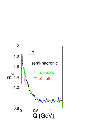
Figure 14: $R_{2}(Q)$ measured by l3 L3 Collab. et al. (2002c) for hadronic W-boson decays from $\mathrm{e^{+}}\mathrm{e^{-}}\kern-3.50006pt\rightarrow\mathrm{W^{+}}\mathrm{W^{-}}\rightarrow\mathrm{q}\mathrm{\overline{q}}\ell\nu$ and hadronic $\mathrm{Z}$-boson decays to all flavors and to udsc flavors only.

Inter-string BEC

A more interesting case is $\mathrm{e^{+}}\mathrm{e^{-}}\kern-3.50006pt\rightarrow\mathrm{W^{+}}\mathrm{W^{-}}\rightarrow\mathrm{q}\mathrm{\overline{q}}\mathrm{q}\mathrm{\overline{q}}$. The $\mathrm{W}$-bosons are produced not far above threshold and consequently travel only about 0.7 fm before decaying. This is smaller than the distance over which hadronization occurs. Therefore one expects a significant degree of overlap of the two hadronizing systems, resulting in BEC not only between particles produced by the same $\mathrm{W}$, but also between particles produced by different $\mathrm{W}$-bosons. On the other hand, in the string picture no BEC is expected between particles arising from different strings.

Whether or not this so-called inter-string BEC exists is thus a fundamental question for the string picture. It is also important for the measurement of properties of the $\mathrm{W}$-boson, in particular its mass Lönnblad and Sjöstrand (1995). Improper simulation of inter-string BEC in Monte Carlo programs would lead to a bias in the mass measurement.

All four lep experiments have studied this question ALEPH Collab. et al. (2000b, 2005b); DELPHI Collab. et al. (1997, 2005); L3 Collab. et al. (2002c); OPAL Collab. et al. (2004). The basic method Chekanov et al. (1999) is to test the expectation of no inter-string BEC. If the two $\mathrm{W}$-bosons decay completely independently, the two-particle density in the 4-quark channel is given by

$${\rho_{\mathrm{4q}}(p_{1},p_{2})}= {\rho^{+}(p_{1},p_{2})} \mathrm{1,2\ from\ \mathrm{W^{+}}}$$

$$+ {\rho^{-}(p_{1},p_{2})} \mathrm{1,2\ from\ \mathrm{W^{-}}}$$

$$+ {\rho^{+}(p_{1})\rho^{-}(p_{2})} \mathrm{1\ from\ \mathrm{W^{+}},\ 2\ from\ \mathrm{W^{-}}}$$

$$+ {\rho^{+}(p_{2})\rho^{-}(p_{1})} \mathrm{1\ from\ \mathrm{W^{-}},\ 2\ from\ \mathrm{W^{+}}.}$$

Assuming $\rho^{+}=\rho^{-}=\rho_{\mathrm{2q}}$, which would only be strictly true if there is complete overlap,

$$\rho_{\mathrm{4q}}(p_{1},p_{2})=2\rho_{\mathrm{2q}}(p_{1},p_{2})+2\rho_{\mathrm{2q}}(p_{1})\rho_{\mathrm{2q}}(p_{2})\ .$$ (25)

The density $\rho_{\mathrm{4q}}(p_{1},p_{2})$ is measured in $\mathrm{e^{+}}\mathrm{e^{-}}\kern-3.50006pt\rightarrow\mathrm{W^{+}}\mathrm{W^{-}}\rightarrow\mathrm{q}\mathrm{\overline{q}}\mathrm{q}\mathrm{\overline{q}}$ and $\rho_{\mathrm{2q}}(p_{1},p_{2})$ in $\mathrm{e^{+}}\mathrm{e^{-}}\kern-3.50006pt\rightarrow\mathrm{W^{+}}\mathrm{W^{-}}\rightarrow\mathrm{q}\mathrm{\overline{q}}\ell\nu$. The remaining term, $\rho_{\mathrm{2q}}(p_{1})\rho_{\mathrm{2q}}(p_{2})$, is estimated by $\rho_{\mathrm{mix}}(p_{1},p_{2})$ obtained by mixing $\ell^{+}\nu\mathrm{q}\mathrm{\overline{q}}$ and $\mathrm{q}\mathrm{\overline{q}}\ell^{-}\nu$ events after removal of the $\ell^{+}$ and $\ell^{-}$. Thus, (25) becomes

$$\rho_{\mathrm{4q}}(Q)=2\rho_{\mathrm{2q}}(Q)+2\rho_{\mathrm{mix}}(Q)\ .$$ (26)

Various quantities are defined to test the validity of (26):

$$\Delta\rho(Q) = \rho_{\mathrm{4q}}(Q)-\left[2{\rho_{\mathrm{2q}}(p_{1},p_{2})}+2{\rho_{\mathrm{mix}}(p_{1},p_{2})}\right]$$ (27)

$$D(Q) = \frac{\rho_{\mathrm{4q}}(Q)}{2\rho_{\mathrm{2q}}(Q)+2\rho_{\mathrm{mix}}(Q)}$$ (28)

$$\delta_{\mathrm{\,I}}(Q) = \frac{\Delta\rho(Q)}{2\rho_{\mathrm{mix}}(Q)}\ .$$ (29)

The quantity $\delta_{\mathrm{\,I}}(Q)$ is actually the correlation function of genuine inter-W BEC De Wolf (2001) and is thus not only a test of no inter-W BEC, but the quantity of interest if inter-W BEC indeed exists.

All four lep experiments have now reported final results ALEPH Collab. et al. (2005b); DELPHI Collab. et al. (2005); L3 Collab. et al. (2002c); OPAL Collab. et al. (2004). Fig. 15 shows results of delphi DELPHI Collab. et al. (2005), the only experiment which claims to have seen significant inter-W BEC. The $\delta_{\mathrm{\,I}}$ distribution of like-sign pions (Fig. 15a) clearly shows an enhancement at small $Q$, while no enhancement is seen in the Monte Carlo distribution where BEC, as modeled by the ${\mathrm{BE}_{32}}$ model Lönnblad and Sjöstrand (1998), is included only between pions from the same $\mathrm{W}$. When pions from different $\mathrm{W}$-bosons are modeled with the same BEC as pions from the same $\mathrm{W}$, a larger enhancement is seen than that of the data.

However, the interpretation of the enhancement in the data as inter-W BEC is somewhat clouded by the observance of an enhancement, albeit smaller, in the $\delta_{\mathrm{\,I}}$ distribution of unlike-sign pions (Fig. 15b). In this distribution the enhancement in the data is larger than that for Monte Carlo with inter-W BEC.

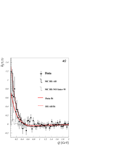
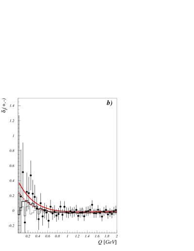
Figure 15: $\delta_{\mathrm{\,I}}(Q)$ measured by delphi DELPHI Collab. et al. (2005) for (a) like- and (b) unlike-sign pion pairs. Also shown are the expectations of Monte Carlo models including BEC among all pions or including BEC only among pions from the same W.

The final results for the four lep experiments are compared in Fig. 16. Here the results are expressed as the ratio of the effect seen to that expected in the ${\mathrm{BE}_{32}}$ model with the same inter-W BEC as intra-W BEC. The measurements indicated by arrows are combined to give the preliminary lep result LEP Electroweak Working Group (2005) of $0.17\pm 0.13$. The data are thus compatible with no inter-W BEC.

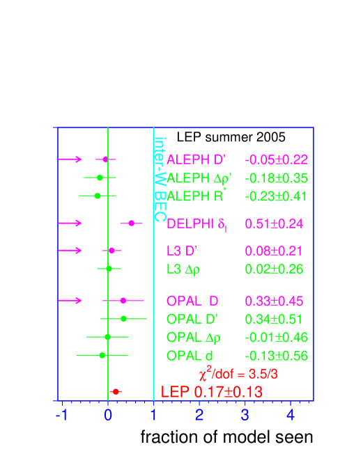
Figure 16: The amount of inter-W BEC observed expressed as a fraction of the prediction of the ${\mathrm{BE}_{32}}$ model. The measurements indicated by arrows are combined to give the preliminary lep result LEP Electroweak Working Group (2005).

3.4 BEC in the Lund string model

In the Lund string model, the longitudinal break-up of the color string is governed by the area law. The matrix element to get a final state depends on the area $A$: ${\cal M}=\exp\left[(\imath\kappa-b/2)A\right]$, where $\kappa$ is the string tension and $b$ is a decay constant with values $\kappa\approx 1$ $\mathrm{G}{\mathrm{e\kern-0.80002ptV}}$/fm and $b\approx 0.3$ $\mathrm{G}{\mathrm{e\kern-0.80002ptV}}$/fm. Consider the string break-up illustrated by the solid line in Fig. 17, which spans the area $A$. Suppose that the particles 1 and 2 are identical. The final state produced by interchanging them would be produced by the string break-up with area $A+\Delta A$. Transverse momentum arises via a tunneling mechanism, which is also related to $b$. To incorporate BEC in the string model, the probability of a final state should be taken as the square of the sum of the matrix elements corresponding to the areas of all the permutations of identical bosons Andersson and Hofmann (1986); Andersson and Ringnér (1998a, b). This model results in BEC, including genuine 3-particle BEC. It predicts that the longitudinal radius is greater than the transverse radius and that the radius for neutral pions is smaller than that for charged pions. In such a model there is no mechanism for creating correlations between particles from different strings.

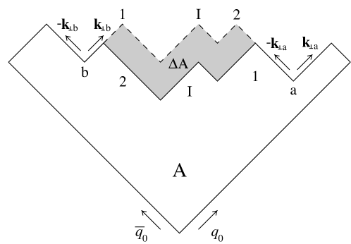
Figure 17: The break-up of a Lund string into hadrons, showing two break-up patterns giving the same final state with two identical particles interchanged..

The model has been incorporated in Monte Carlo for a $\mathrm{q}$$\mathrm{\overline{q}}$ string. While the formalism to do so for the more realistic case of a string with multiple gluons has been worked out Andersson et al. (2001), a successful Monte Carlo implementation has, unfortunately, so far proved elusive.

4 Conclusions

We have seen that the study of BEC in $\mathrm{e^{+}}$$\mathrm{e^{-}}$ presents a number of problems, both experimental and theoretical. Consequently, values obtained for parameters vary considerably among experiments, even when the same parametrization is used. Nevertheless, certain features are clear: BEC, both 2-particle and genuine 3-particle, exist; they seem independent of center-of-mass energy; the source shape is somewhat elongated in the jet direction; and the (Fermi-Dirac) radius for baryons is smaller than the radius for mesons. Experimentally, it is not clear whether the radius for neutral pions is smaller than that for charged pions. BEC in W decay is the same as in light-quark Z decay. The data are compatible with no inter-W BEC.

The implementation of BEC in the Lund string model appears consistent with these experimental findings. However, the experimental evidence that pion production is completely incoherent seems at odds with the coherent addition of amplitudes in the model.

References

- Goldhaber et al. (1960) G. Goldhaber, S. Goldhaber, W. Lee, and A. Pais, Phys. Rev. 120, 300–312 (1960).
- Boal et al. (1990) D. H. Boal, C.-K. Gelbke, and B. K. Jennings, Rev. Mod. Phys. 62, 553–602 (1990).
- Edgeworth (1905) F. Edgeworth, Trans. Cambridge Phil. Soc. 20, 36 (1905), see also Harald Cramér, Mathematical Methods of Statistics, Princeton Univ. Press, 1946.
- Gyulassy et al. (1979) M. Gyulassy, S. Kauffmann, and L. W. Wilson, Phys. Rev. C20, 2267–2292 (1979).
- Osada et al. (1996) T. Osada, S. Sano, and M. Biyajima, Z. Phys. C72, 285–290 (1996).
- ALEPH Collab. et al. (1992) ALEPH Collab., D. Decamp, et al., Z. Phys. C54, 75–85 (1992).
- ALEPH Collab. et al. (2004) ALEPH Collab., A. Heister, et al., Eur. Phys. J. C36, 147–159 (2004).
- DELPHI Collab. et al. (1992) DELPHI Collab., P. Abreu, et al., Phys. Lett. B286, 201–210 (1992).
- L3 Collab. et al. (2002a) L3 Collab., P. Achard, et al., Phys. Lett. B540, 185–198 (2002a).
- OPAL Collab. et al. (1991) OPAL Collab., P. Acton, et al., Phys. Lett. B267, 143–153 (1991).
- OPAL Collab. et al. (1996a) OPAL Collab., G. Alexander, et al., Z. Phys. C72, 389–398 (1996a).
- OPAL Collab. et al. (2000) OPAL Collab., G. Abbiendi, et al., Eur. Phys. J. C16, 423–433 (2000).
- Aihara et al. (1985) H. Aihara, et al., Phys. Rev. D31, 996–1003 (1985).
- Juricic et al. (1989) I. Juricic, et al., Phys. Rev. D39, 1–20 (1989).
- TASSO Collab. et al. (1986) M. A. TASSO Collab., et al., Z. Phys. C30, 355–369 (1986).
- AMY Collab. et al. (1995) S. C. AMY Collab., et al., Phys. Lett. B355, 406–414 (1995).
- Alexander (2003) G. Alexander, Rep. Prog. Phys. 66, 481–522 (2003).
- DELPHI Collab. et al. (1996) DELPHI Collab., P. Abreu, et al., Phys. Lett. B379, 330–340 (1996).
- OPAL Collab. et al. (2001) OPAL Collab., G. Abbiendi, et al., Eur. Phys. J. C21, 23–32 (2001).
- ALEPH Collab. et al. (2005a) ALEPH Collab., S. Schael, et al., Phys. Lett. B611, 66–80 (2005a).
- OPAL Collab. et al. (1995) OPAL Collab., R. Akers, et al., Z. Phys. C67, 389–401 (1995).
- ALEPH Collab. et al. (2000a) ALEPH Collab., R. Barate, et al., Phys. Lett. B475, 395–406 (2000a).
- OPAL Collab. et al. (1996b) OPAL Collab., G. Alexander, et al., Phys. Lett. B384, 377–387 (1996b).
- L3 Collab. et al. (1999) L3 Collab., M. Acciarri, et al., Phys. Lett. B458, 517–528 (1999).
- DELPHI Collab. et al. (2000) DELPHI Collab., P. Abreu, et al., Phys. Lett. B471, 460–470 (2000).
- ZEUS Collab. et al. (2004) ZEUS Collab., S. Chekanov, et al., Phys. Lett. B583, 231–246 (2004).
- L3 Collab. et al. (2002b) L3 Collab., P. Achard, et al., Phys. Lett. B524, 55–64 (2002b).
- OPAL Collab. et al. (2003) OPAL Collab., G. Abbiendi, et al., Phys. Lett. B559, 131–143 (2003).
- Lörstad (1989) B. Lörstad, Int. J. Mod. Phys. A4, 2861–2896 (1989).
- Lyuboshitz (1991) V. Lyuboshitz, Sov. J. Nucl. Phys. 53, 514–2896 (1991).
- DELPHI Collab. et al. (1995) DELPHI Collab., P. Abreu, et al., Phys. Lett. B355, 415–424 (1995).
- OPAL Collab. et al. (1996c) OPAL Collab., K. Ackerstaff, et al., Eur. Phys. J. C5, 239–248 (1996c).
- ALEPH Collab. et al. (2000b) ALEPH Collab., R. Barate, et al., Phys. Lett. B478, 50–64 (2000b).
- L3 Collab. et al. (2002c) L3 Collab., P. Achard, et al., Phys. Lett. B547, 139–150 (2002c).
- Lönnblad and Sjöstrand (1995) L. Lönnblad, and T. Sjöstrand, Phys. Lett. B351, 293–301 (1995).
- ALEPH Collab. et al. (2005b) ALEPH Collab., S. Schael, et al., Phys. Lett. B606, 265–275 (2005b).
- DELPHI Collab. et al. (1997) DELPHI Collab., P. Abreu, et al., Phys. Lett. B401, 181–191 (1997).
- DELPHI Collab. et al. (2005) DELPHI Collab., J. Abdallah, et al., Eur. Phys. J. C44, 161–174 (2005).
- OPAL Collab. et al. (2004) OPAL Collab., G. Abbiendi, et al., Eur. Phys. J. C36, 297–308 (2004).
- Chekanov et al. (1999) S. Chekanov, E. De Wolf, and W. Kittel, Eur. Phys. J. C6, 403–411 (1999).
- De Wolf (2001) E. De Wolf, Correlations in hadronic decays (2001).
- Lönnblad and Sjöstrand (1998) L. Lönnblad, and T. Sjöstrand, Eur. Phys. J. C2, 165–180 (1998).
- LEP Electroweak Working Group (2005) LEP Electroweak Working Group, A Combination of Preliminary Electroweak Measurements and Constraints on the Standard Model, Tech. Rep. LEPEWWG/2005-01 (2005).
- Andersson and Hofmann (1986) B. Andersson, and W. Hofmann, Phys. Lett. B169, 364–368 (1986).
- Andersson and Ringnér (1998a) B. Andersson, and M. Ringnér, Nucl. Phys. B513, 627–644 (1998a).
- Andersson and Ringnér (1998b) B. Andersson, and M. Ringnér, Phys. Lett. B421, 283–288 (1998b).
- Andersson et al. (2001) B. Andersson, S. Mohanty, and F. Söderberg, Eur. Phys. J. C21, 631–647 (2001).