EUROPEAN ORGANIZATION FOR NUCLEAR RESEARCH

OPAL PR 410

CERN-PH-EP/2005-038

15 th July 2005

Measurement of the mass and width of the W boson

The OPAL Collaboration

The mass and width of the W boson are measured using $\mbox{$\rm e^{+}e^{-}$}\rightarrow\mbox{$\rm W^{+}W^{-}$}$ events from the data sample collected by the OPAL experiment at LEP at centre-of-mass energies between 170 GeV and 209 GeV. The mass ($m_{\rm W}$) and width ($\Gamma_{\rm W}$) are determined using direct reconstruction of the kinematics of $\mbox{$\rm W^{+}W^{-}$}\rightarrow\mbox{$\rm q\bar{q}\ell\nu$}$ and $\mbox{$\rm W^{+}W^{-}$}\rightarrow\mbox{$\rm q\bar{q}q\bar{q}$}$ events. When combined with previous OPAL measurements using $\mbox{$\rm W^{+}W^{-}$}\rightarrow\mbox{$\rm\ell\nu\ell\nu$}$ events and the dependence on $m_{\rm W}$ of the WW production cross-section at threshold, the results are determined to be

$$m_{\rm W} = 80.415\pm 0.042\pm 0.030\pm 0.009\rm\,GeV$$

$$\Gamma_{\rm W} = 1.996\pm 0.096\pm 0.102\pm 0.003\rm\,GeV$$

where the first error is statistical, the second systematic and the third due to uncertainties in the value of the LEP beam energy. By measuring $m_{\rm W}$ with several different jet algorithms in the $\rm q\bar{q}q\bar{q}$ channel, a limit is also obtained on possible final-state interactions due to colour reconnection effects in $\mbox{$\rm W^{+}W^{-}$}\rightarrow\mbox{$\rm q\bar{q}q\bar{q}$}$ events. The consistency of the results for the W mass and width with those inferred from other electroweak parameters provides an important test of the Standard Model of electroweak interactions.

This paper is dedicated to the memory of Steve O’Neale

Submitted to Eur. Phys. J. C.

The OPAL Collaboration

G. Abbiendi², C. Ainsley⁵, P.F. Åkesson^3,y, G. Alexander²², G. Anagnostou¹, K.J. Anderson⁹, S. Asai²³, D. Axen²⁷, I. Bailey²⁶, E. Barberio^8,p, T. Barillari³², R.J. Barlow¹⁶, R.J. Batley⁵, P. Bechtle²⁵, T. Behnke²⁵, K.W. Bell²⁰, P.J. Bell¹, G. Bella²², A. Bellerive⁶, G. Benelli⁴, S. Bethke³², O. Biebel³¹, O. Boeriu¹⁰, P. Bock¹¹, M. Boutemeur³¹, S. Braibant², R.M. Brown²⁰, H.J. Burckhart⁸, S. Campana⁴, P. Capiluppi², R.K. Carnegie⁶, A.A. Carter¹³, J.R. Carter⁵, C.Y. Chang¹⁷, D.G. Charlton¹, C. Ciocca², A. Csilling²⁹, M. Cuffiani², S. Dado²¹, A. De Roeck⁸, E.A. De Wolf^8,s, K. Desch²⁵, B. Dienes³⁰, J. Dubbert³¹, E. Duchovni²⁴, G. Duckeck³¹, I.P. Duerdoth¹⁶, E. Etzion²², F. Fabbri², P. Ferrari⁸, F. Fiedler³¹, I. Fleck¹⁰, M. Ford¹⁶, A. Frey⁸, P. Gagnon¹², J.W. Gary⁴, C. Geich-Gimbel³, G. Giacomelli², P. Giacomelli², M. Giunta⁴, J. Goldberg²¹, E. Gross²⁴, J. Grunhaus²², M. Gruwé⁸, P.O. Günther³, A. Gupta⁹, C. Hajdu²⁹, M. Hamann²⁵, G.G. Hanson⁴, A. Harel²¹, M. Hauschild⁸, C.M. Hawkes¹, R. Hawkings⁸, R.J. Hemingway⁶, G. Herten¹⁰, R.D. Heuer²⁵, J.C. Hill⁵, D. Horváth^29,c, P. Igo-Kemenes¹¹, K. Ishii²³, H. Jeremie¹⁸, P. Jovanovic¹, T.R. Junk^6,i, J. Kanzaki^23,u, D. Karlen²⁶, K. Kawagoe²³, T. Kawamoto²³, R.K. Keeler²⁶, R.G. Kellogg¹⁷, B.W. Kennedy²⁰, S. Kluth³², T. Kobayashi²³, M. Kobel³, S. Komamiya²³, T. Krämer²⁵, A. Krasznahorkay^30,e, P. Krieger^6,l, J. von Krogh¹¹, T. Kuhl²⁵, M. Kupper²⁴, G.D. Lafferty¹⁶, H. Landsman²¹, D. Lanske¹⁴, D. Lellouch²⁴, J. Letts^o, L. Levinson²⁴, J. Lillich¹⁰, S.L. Lloyd¹³, F.K. Loebinger¹⁶, J. Lu^27,w, A. Ludwig³, J. Ludwig¹⁰, W. Mader^3,b, S. Marcellini², A.J. Martin¹³, T. Mashimo²³, P. Mättig^m, J. McKenna²⁷, R.A. McPherson²⁶, F. Meijers⁸, W. Menges²⁵, F.S. Merritt⁹, H. Mes^6,a, N. Meyer²⁵, A. Michelini², S. Mihara²³, G. Mikenberg²⁴, D.J. Miller¹⁵, W. Mohr¹⁰, T. Mori²³, A. Mutter¹⁰, K. Nagai¹³, I. Nakamura^23,v, H. Nanjo²³, H.A. Neal³³, R. Nisius³², S.W. O’Neale^1,∗, A. Oh⁸, M.J. Oreglia⁹, S. Orito^23,∗, C. Pahl³², G. Pásztor^4,g, J.R. Pater¹⁶, J.E. Pilcher⁹, J. Pinfold²⁸, D.E. Plane⁸, O. Pooth¹⁴, M. Przybycień^8,n, A. Quadt³, K. Rabbertz^8,r, C. Rembser⁸, P. Renkel²⁴, J.M. Roney²⁶, A.M. Rossi², Y. Rozen²¹, K. Runge¹⁰, K. Sachs⁶, T. Saeki²³, E.K.G. Sarkisyan^8,j, A.D. Schaile³¹, O. Schaile³¹, P. Scharff-Hansen⁸, J. Schieck³², T. Schörner-Sadenius^8,z, M. Schröder⁸, M. Schumacher³, R. Seuster^14,f, T.G. Shears^8,h, B.C. Shen⁴, P. Sherwood¹⁵, A. Skuja¹⁷, A.M. Smith⁸, R. Sobie²⁶, S. Söldner-Rembold¹⁶, F. Spano^9,y, A. Stahl^3,x, D. Strom¹⁹, R. Ströhmer³¹, S. Tarem²¹, M. Tasevsky^8,d, R. Teuscher⁹, M.A. Thomson⁵, E. Torrence¹⁹, D. Toya²³, P. Tran⁴, I. Trigger⁸, Z. Trócsányi^30,e, E. Tsur²², M.F. Turner-Watson¹, I. Ueda²³, B. Ujvári^30,e, C.F. Vollmer³¹, P. Vannerem¹⁰, R. Vértesi^30,e, M. Verzocchi¹⁷, H. Voss^8,q, J. Vossebeld^8,h, C.P. Ward⁵, D.R. Ward⁵, P.M. Watkins¹, A.T. Watson¹, N.K. Watson¹, P.S. Wells⁸, T. Wengler⁸, N. Wermes³, G.W. Wilson^16,k, J.A. Wilson¹, G. Wolf²⁴, T.R. Wyatt¹⁶, S. Yamashita²³, D. Zer-Zion⁴, L. Zivkovic²⁴

¹School of Physics and Astronomy, University of Birmingham, Birmingham B15 2TT, UK
²Dipartimento di Fisica dell’ Università di Bologna and INFN, I-40126 Bologna, Italy
³Physikalisches Institut, Universität Bonn, D-53115 Bonn, Germany
⁴Department of Physics, University of California, Riverside CA 92521, USA
⁵Cavendish Laboratory, Cambridge CB3 0HE, UK
⁶Ottawa-Carleton Institute for Physics, Department of Physics, Carleton University, Ottawa, Ontario K1S 5B6, Canada
⁸CERN, European Organisation for Nuclear Research, CH-1211 Geneva 23, Switzerland
⁹Enrico Fermi Institute and Department of Physics, University of Chicago, Chicago IL 60637, USA
¹⁰Fakultät für Physik, Albert-Ludwigs-Universität Freiburg, D-79104 Freiburg, Germany
¹¹Physikalisches Institut, Universität Heidelberg, D-69120 Heidelberg, Germany
¹²Indiana University, Department of Physics, Bloomington IN 47405, USA
¹³Queen Mary and Westfield College, University of London, London E1 4NS, UK
¹⁴Technische Hochschule Aachen, III Physikalisches Institut, Sommerfeldstrasse 26-28, D-52056 Aachen, Germany
¹⁵University College London, London WC1E 6BT, UK
¹⁶Department of Physics, Schuster Laboratory, The University, Manchester M13 9PL, UK
¹⁷Department of Physics, University of Maryland, College Park, MD 20742, USA
¹⁸Laboratoire de Physique Nucléaire, Université de Montréal, Montréal, Québec H3C 3J7, Canada
¹⁹University of Oregon, Department of Physics, Eugene OR 97403, USA
²⁰CCLRC Rutherford Appleton Laboratory, Chilton, Didcot, Oxfordshire OX11 0QX, UK
²¹Department of Physics, Technion-Israel Institute of Technology, Haifa 32000, Israel
²²Department of Physics and Astronomy, Tel Aviv University, Tel Aviv 69978, Israel
²³International Centre for Elementary Particle Physics and Department of Physics, University of Tokyo, Tokyo 113-0033, and Kobe University, Kobe 657-8501, Japan
²⁴Particle Physics Department, Weizmann Institute of Science, Rehovot 76100, Israel
²⁵Universität Hamburg/DESY, Institut für Experimentalphysik, Notkestrasse 85, D-22607 Hamburg, Germany
²⁶University of Victoria, Department of Physics, P O Box 3055, Victoria BC V8W 3P6, Canada
²⁷University of British Columbia, Department of Physics, Vancouver BC V6T 1Z1, Canada
²⁸University of Alberta, Department of Physics, Edmonton AB T6G 2J1, Canada
²⁹Research Institute for Particle and Nuclear Physics, H-1525 Budapest, P O Box 49, Hungary
³⁰Institute of Nuclear Research, H-4001 Debrecen, P O Box 51, Hungary
³¹Ludwig-Maximilians-Universität München, Sektion Physik, Am Coulombwall 1, D-85748 Garching, Germany
³²Max-Planck-Institute für Physik, Föhringer Ring 6, D-80805 München, Germany
³³Yale University, Department of Physics, New Haven, CT 06520, USA

^a and at TRIUMF, Vancouver, Canada V6T 2A3
^b now at University of Iowa, Dept of Physics and Astronomy, Iowa, U.S.A.
^c and Institute of Nuclear Research, Debrecen, Hungary
^d now at Institute of Physics, Academy of Sciences of the Czech Republic, 18221 Prague, Czech Republic
^e and Department of Experimental Physics, University of Debrecen, Hungary
^f and MPI München
^g and Research Institute for Particle and Nuclear Physics, Budapest, Hungary
^h now at University of Liverpool, Dept of Physics, Liverpool L69 3BX, U.K.
ⁱ now at Dept. Physics, University of Illinois at Urbana-Champaign, U.S.A.
^j and Manchester University Manchester, M13 9PL, United Kingdom
^k now at University of Kansas, Dept of Physics and Astronomy, Lawrence, KS 66045, U.S.A.
^l now at University of Toronto, Dept of Physics, Toronto, Canada
^m current address Bergische Universität, Wuppertal, Germany
ⁿ now at University of Mining and Metallurgy, Cracow, Poland
^o now at University of California, San Diego, U.S.A.
^p now at The University of Melbourne, Victoria, Australia
^q now at IPHE Université de Lausanne, CH-1015 Lausanne, Switzerland
^r now at IEKP Universität Karlsruhe, Germany
^s now at University of Antwerpen, Physics Department,B-2610 Antwerpen, Belgium; supported by Interuniversity Attraction Poles Programme – Belgian Science Policy
^u and High Energy Accelerator Research Organisation (KEK), Tsukuba, Ibaraki, Japan
^v now at University of Pennsylvania, Philadelphia, Pennsylvania, USA
^w now at TRIUMF, Vancouver, Canada
^x now at DESY Zeuthen
^y now at CERN
^z now at DESY
^∗ Deceased

1 Introduction

The measurement of the mass of the W boson ($m_{\rm W}$) is one of the principal goals of the physics programme undertaken with the LEP $\rm e^{+}e^{-}$ collider at CERN. Within the Standard Model of electroweak interactions, the W mass can be inferred indirectly from precision measurements of electroweak observables, in particular from $\mbox{$\rm e^{+}e^{-}$}\rightarrow\mbox{$\rm Z$}$ events at centre-of-mass energies ($\sqrt{s}$) close to the peak of the Z resonance (around 91 GeV), studied extensively at LEP1 and SLD [1]. These measurements currently give a prediction for $m_{\rm W}$ with an uncertainty of 32 MeV, or 23 MeV if the measurement of the mass of the top quark from the Tevatron [2] is also taken into account. Direct measurements of the W mass with a similar precision are therefore of great interest, both to test the consistency of the Standard Model and better to constrain its parameters (for example the mass of the so-far unobserved Higgs boson), and to look for deviations signalling the possible presence of new physics beyond the Standard Model. Such measurements became possible at LEP once the centre-of-mass energy was raised above 160 GeV in 1996, allowing the production of pairs of W bosons in the reaction $\mbox{$\rm e^{+}e^{-}$}\rightarrow\mbox{$\rm W^{+}W^{-}$}$. Measurements of the width of the W boson ($\Gamma_{\rm W}$) can also be carried out at LEP, providing a further test of the consistency of the Standard Model.

This paper presents the final OPAL measurement of the mass and width of the W boson, using direct reconstruction of the two boson masses in $\mbox{$\rm e^{+}e^{-}$}\rightarrow\mbox{$\rm W^{+}W^{-}$}\rightarrow\mbox{$\rm q\bar{q}\ell\nu$}$ and $\rm q\bar{q}q\bar{q}$ events recorded at $\rm e^{+}e^{-}$ collision energies between 170 GeV and 209 GeV. The result for $m_{\rm W}$ is combined with a measurement using direct reconstruction in the $\rm\ell\nu\ell\nu$ final state [3] and a measurement from the dependence of the WW production cross-section on $m_{\rm W}$ at $\sqrt{s}\approx 161$ GeV [4]. This paper supersedes our previous results [5, 6, 7] obtained from the data with $\mbox{$\sqrt{s}$}=$170–189 GeV.

Three methods are used in this paper to extract $m_{\rm W}$, all based on similar kinematic fits to the reconstructed jets and leptons in each event. The principal method, the convolution fit, is based on an event-by-event convolution of a resolution function, describing the consistency of the event kinematics with various W boson mass hypotheses, with a Breit-Wigner physics function dependent on the assumed true W boson mass and width. The convolution fit is used to obtain the central results of this paper, but is complemented by two other fit methods of slightly lower statistical precision: a reweighting fit based on fitting Monte Carlo template distributions with varying assumed W mass and width to the reconstructed data distributions, and a simple analytic Breit-Wigner fit to the distribution of reconstructed W boson masses in the data. Complete analyses, including systematic uncertainties, have been performed for all three methods, providing valuable cross-checks of all stages of the analysis procedure. The convolution and reweighting fits also measure the W width; the convolution fit is again used for the central results, and the reweighting fit provides a cross-check including all systematic uncertainties. The Breit-Wigner fit does not measure the W width, but an additional independent convolution-based method is used to provide a second statistical cross-check in the $\rm q\bar{q}\ell\nu$ channel.

The dominant systematic error in the $\rm q\bar{q}q\bar{q}$ channel comes from possible final-state interactions (colour reconnection and Bose-Einstein correlations) between the decay products of the two hadronically decaying W bosons. According to present phenomenological models, these interactions mainly affect soft particles, and the uncertainties can be reduced by removing or deweighting soft particles when estimating the directions of jets. Such a method is used for the $\rm q\bar{q}q\bar{q}$ channel measurements of $m_{\rm W}$ from all three fit methods in this paper. Conversely, the effect of final-state interactions can be enhanced by giving increased weight to soft particles, and this is used to place constraints on possible colour reconnection effects.

This paper is organised as follows. The OPAL detector, data and Monte Carlo samples are introduced in Section 2, followed by a brief description of the event selection in Section 3. Elements of the event reconstruction and kinematic fitting common to all three analysis methods are discussed in Section 4, followed by a detailed description of the individual convolution, reweighting and Breit-Wigner fits in Sections 5–7. Systematic uncertainties, which are largely common to all three methods, are described in Section 8. Finally the results are summarised in Sections 9 and 10.

2 Data and Monte Carlo samples

A detailed description of the OPAL detector can be found elsewhere [8]. Tracking of charged particles was performed by a central detector, enclosed in a solenoid which provided a uniform axial magnetic field of 0.435 T. The central detector consisted of a two-layer silicon microvertex detector, a high precision vertex chamber with both axial and stereo wire layers, a large volume jet chamber providing both tracking and ionisation energy loss information, and additional chambers to measure the $z$ coordinate of tracks as they left the central detector. Together these detectors provided tracking coverage for polar angles $|\cos\theta|<0.96$, with a typical transverse momentum ($p_{\rm T}$) resolution of $\sigma_{p_{\rm T}}/p_{\rm T}=\sqrt{(0.02)^{2}+(0.0015p_{T})^{2}}$ with $p_{\rm T}$ measured in GeV. The solenoid coil was surrounded by a time-of-flight counter array and a barrel lead-glass electromagnetic calorimeter with a presampler. Including also the endcap electromagnetic calorimeters, the lead-glass blocks covered the range $|\cos\theta|<0.98$ with a granularity of about $2.3^{\circ}$ in both $\theta$ and $\phi$. Outside the electromagnetic calorimetry, the magnet return yoke was instrumented with streamer tubes to form a hadronic calorimeter, with angular coverage in the range $|\cos\theta|<0.91$ and a granularity of about $5^{\circ}$ in $\theta$ and $7.5^{\circ}$ in $\phi$. The region $0.91<|\cos\theta|<0.99$ was instrumented with an additional pole-tip hadronic calorimeter using multi-wire chambers, having a granularity of about $4^{\circ}$ in $\theta$ and $11^{\circ}$ in $\phi$. The detector was completed with muon detectors outside the magnet return yoke. These were composed of drift chambers in the barrel region and limited streamer tubes in the endcaps, and together covered 93 % of the full solid angle. The integrated luminosity was evaluated using small angle Bhabha scattering events observed in the forward calorimeters [9].

The data used for this analysis were taken at centre-of-mass energies between 170 GeV and 209 GeV during the LEP2 running period from 1996 to 2000, and correspond to a total integrated luminosity of about 689 $\rm pb^{-1}$. In the year 2000, LEP was operated in a mode where the beam energy was increased in $\sim 0.5$ GeV steps during data taking several times in each collider fill. Data taken during these ‘miniramps’ (approximately 1 % of the total year 2000 data sample) are excluded from the analysis as the beam energy is not precisely known. A detailed breakdown of the energy ranges and integrated luminosities in each year of data taking is given in Table 1. In addition, $\mbox{$\rm e^{+}e^{-}$}\rightarrow\mbox{$\rm Z$}$ events recorded at $\sqrt{s}\approx 91$ GeV were used to calibrate the leptonic and hadronic energy scales and to study the modelling of the detector response by the Monte Carlo simulation. These events were recorded during dedicated runs at the beginning of each year, and also at intervals later in the data-taking periods to monitor the stability of the detector performance with time. They amount to a total integrated luminosity of about 13 $\rm pb^{-1}$, corresponding for example to about 400 000 hadronic $\rm Z$ decays.

Year	$\sqrt{s}$ range	$\langle{\mbox{$\sqrt{s}$}}\rangle$	$\int L$ dt	$\rm q\bar{q}e\nu$		$\rm q\bar{q}\mu\nu$		$\rm q\bar{q}\tau\nu$		$\rm q\bar{q}q\bar{q}$
	(GeV)	(GeV)	(pb-1)	obs.	exp.	obs.	exp.	obs.	exp.	obs.	exp.
1996	170–173	172.1	10.4	22	20	15	19	13	10	60	58
1997	181–184	182.7	57.4	134	122	117	124	118	124	437	446
1998	188–189	188.6	183.1	388	413	422	417	444	425	1551	1511
1999	192–202	197.4	218.5	524	512	489	518	559	526	1924	1891
2000	200–209	206.0	219.6	506	524	530	525	555	543	1921	1925
Total	170–209	196.2	688.9	1574	1591	1573	1603	1689	1628	5893	5831
Estimated selection efficiency (%)					85		89		68		86
Estimated purity (%)					92		92		73		79

Table 1: Observed and expected numbers of candidate WW events, together with the collision energy range, mean energy and integrated luminosity, in each year of data taking. The efficiencies and purities of the event selections, estimated from Monte Carlo events, are also given.

Large samples of Monte Carlo simulated events have been generated to optimise and calibrate the W mass and width analysis methods, and to study systematic uncertainties. The relevant contributions to the $\mbox{$\rm e^{+}e^{-}$}\rightarrow\mbox{$\rm q\bar{q}\ell\nu$}$ and $\rm q\bar{q}q\bar{q}$ topologies studied in this paper can be divided into four-fermion and two-fermion processes [10]. As defined here, four-fermion final states ($\mbox{$\rm e^{+}e^{-}$}\rightarrow 4\rm f$) include contributions from both $\mbox{$\rm e^{+}e^{-}$}\rightarrow\mbox{$\rm W^{+}W^{-}$}\rightarrow 4\rm f$ and $\mbox{$\rm e^{+}e^{-}$}\rightarrow\mbox{$\rm ZZ$}\rightarrow 4\rm f$, but exclude multi-peripheral diagrams resulting from two-photon interactions, which have a negligible probability of being selected by the analysis requirements and are not considered further. Most four-fermion final states were simulated using the KoralW 1.42 program [11], which uses matrix elements calculated with grc4f 2.0 [12]. These samples were split into two parts, corresponding to four-fermion final states which could have been produced from diagrams involving at least one W boson (referred to collectively as WW events below), and others (referred to as $\rm ZZ$ events, but including some diagrams not involving two Z bosons). Most WW events were generated with $\mbox{$m_{\rm W}$}=80.33$ GeV and $\mbox{$\Gamma_{\rm W}$}=2.09$ GeV, but samples with other W masses and widths were also produced in order to calibrate and test the fitting procedures. The running width scheme for the Breit-Wigner distribution as implemented in KoralW was used throughout. Four-fermion background from the process $\mbox{$\rm e^{+}e^{-}$}\rightarrow\mbox{$\rm e^{+}e^{-}$}\mbox{$\rm q\bar{q}$}$ (included in the $\rm ZZ$ sample) was simulated using grc4f. The only important two-fermion background process is $\mbox{$\rm e^{+}e^{-}$}\rightarrow\mbox{$\mbox{$\rm Z$}/\gamma$}\rightarrow\mbox{$\rm q\bar{q}$}$, generated using KK2f 4.13 [13], with Pythia 6.125 [14] as an alternative.

Hadronisation of final states involving quarks was performed using the Jetset 7.4 model [15], with parameters tuned by OPAL to describe global event shape and particle production data at the Z resonance [16]. This hadronisation model and parameter set is denoted by JT. To study systematic uncertainties related to hadronisation, the same two- and four-fermion events have been hadronised with various alternative hadronisation models and parameter sets: Jetset 7.4 with an earlier OPAL-tuned parameter set based primarily on event shapes [17] (denoted JT^′), Ariadne 4.08 [18] with parameters tuned to ALEPH data [19] (denoted by AR), Ariadne 4.11 (AR^′) and Herwig 6.2 [20] (HW), both with parameters tuned to OPAL data. The possible effects of final-state interactions in $\mbox{$\rm e^{+}e^{-}$}\rightarrow\mbox{$\rm W^{+}W^{-}$}\rightarrow\mbox{$\rm q\bar{q}q\bar{q}$}$ events have been studied using colour reconnection models implemented in Pythia, Ariadne and Herwig, and the LUBOEI Bose-Einstein correlation model [21] implemented in Pythia, as discussed in Section 8.3. The effects of so-called $O(\alpha)$ photon radiation have been studied using the KandY generator scheme [22], which uses YFSWW3 [23] and KoralW 1.51 [22] running concurrently, as discussed in detail in Section 8.4.

All Monte Carlo samples have been passed through a complete simulation of the OPAL detector [24] and the same reconstruction and analysis algorithms as the real data. Small corrections were applied to the reconstructed jet and lepton four-vectors in Monte Carlo events better to model the energy scales and resolutions seen in data, as discussed in detail in Section 8.1.

3 Event selection

The selections of $\mbox{$\rm W^{+}W^{-}$}\rightarrow\mbox{$\rm q\bar{q}\ell\nu$}$ and $\mbox{$\rm W^{+}W^{-}$}\rightarrow\mbox{$\rm q\bar{q}q\bar{q}$}$ events are based on multivariate relative likelihood discriminants, and are discussed in detail in [25]. Events selected by the $\mbox{$\rm W^{+}W^{-}$}\rightarrow\mbox{$\rm\ell\nu\ell\nu$}$ selection of [25] are rejected, and events selected as both $\rm q\bar{q}\ell\nu$ and $\rm q\bar{q}q\bar{q}$ candidates are retained only for the $\rm q\bar{q}\ell\nu$ analysis. The sets of reference histograms used in the selections have been extended to maintain optimal performance for the highest energy LEP2 running.

Semileptonic $\mbox{$\rm W^{+}W^{-}$}\rightarrow\mbox{$\rm q\bar{q}\ell\nu$}$ decays comprise 44 % of the total WW cross-section, and are selected using separate likelihood discriminants for the $\rm q\bar{q}e\nu$, $\rm q\bar{q}\mu\nu$ and $\rm q\bar{q}\tau\nu$ channels. These events are characterised by two well-separated hadronic jets, large missing momentum due to the escaping neutrino from the leptonic W decay, and in the case of $\rm q\bar{q}e\nu$ and $\rm q\bar{q}\mu\nu$ decays, an isolated high-momentum charged lepton. In $\mbox{$\rm W^{+}W^{-}$}\rightarrow\mbox{$\rm q\bar{q}\tau\nu$}$ events, the $\tau$-lepton is identified as an isolated low multiplicity jet, typically containing one or three tracks. A small number of ‘trackless-lepton’ $\rm q\bar{q}e\nu$ and $\rm q\bar{q}\mu\nu$ events are also selected, where the lepton is identified based on calorimeter and muon chamber information only, without an associated track. These events make up 2.5 % of the $\rm q\bar{q}e\nu$ and 4.7 % of the $\rm q\bar{q}\mu\nu$ samples. Hadronic $\mbox{$\rm W^{+}W^{-}$}\rightarrow\mbox{$\rm q\bar{q}q\bar{q}$}$ decays comprise 46 % of the total WW cross-section, and are characterised by four energetic hadronic jets and little or no missing energy. The dominant background results from $\mbox{$\rm e^{+}e^{-}$}\rightarrow\mbox{$\mbox{$\rm Z$}/\gamma$}\rightarrow\mbox{$\rm q\bar{q}$}$ events giving a four-jet topology ($\mbox{$\rm q\bar{q}$}\rightarrow\mbox{$\rm q\bar{q}q\bar{q}$}$ or $\rm q\bar{q}gg$), and this is largely rejected using an event weight based on the $O(\alpha_{s}^{2})$ QCD matrix element for this background process.

The number of events selected in each of the channels and data-taking years is given in Table 1, together with the expectation from the Monte Carlo simulation with the WW production cross-section scaled to the prediction of KandY (which is more accurate than that of KoralW). The average selection efficiency and purity of each channel in the desired WW signal topology are also given, estimated from Monte Carlo events and averaged over all centre-of-mass energies. The dominant backgrounds are events misclassified between the $\mbox{$\rm q\bar{q}e\nu$}/\mbox{$\rm q\bar{q}\mu\nu$}$ and $\rm q\bar{q}\tau\nu$ channels in the $\rm q\bar{q}\ell\nu$ selection, and $\mbox{$\rm e^{+}e^{-}$}\rightarrow\mbox{$\mbox{$\rm Z$}/\gamma$}\rightarrow\mbox{$\rm q\bar{q}$}$ events giving a four-jet topology in the $\rm q\bar{q}q\bar{q}$ channel. Combining all three $\rm q\bar{q}\ell\nu$ sub-channels, and including events mis-classified between them, 87 % of $\rm q\bar{q}\ell\nu$ events are selected for the mass and width analyses. However, not all selected events are actually used by each analysis—some poorly reconstructed events are removed by analysis-specific cuts as discussed below.

4 W boson reconstruction and kinematic fitting

All three analysis methods use similar event reconstruction and kinematic fit techniques to determine the W mass on an event by event basis. In $\mbox{$\rm W^{+}W^{-}$}\rightarrow\mbox{$\rm q\bar{q}\ell\nu$}$ events, the procedure begins by removing the tracks, electromagnetic and hadronic calorimeter clusters corresponding to the lepton identified by the event selection. A matching algorithm is then applied to tracks and calorimeter clusters, and the cluster energies are adjusted both to compensate for the expected energy sharing between the electromagnetic and hadronic calorimeters, and to account for the expected energy deposits from any associated tracks. This procedure has been optimised to obtain the best possible jet energy resolution on $\mbox{$\rm Z$}\rightarrow\mbox{$\rm q\bar{q}$}$ events at $\mbox{$\sqrt{s}$}\approx 91$ GeV, where use of the hadronic as well as the electromagnetic calorimeter information improves the energy resolution by about 10 %. The reconstructed objects (referred to hereafter as particles) are then grouped into two jets using the Durham jet-finding algorithm [26]. Estimates of the jet energies, directions and masses are derived from the four-momentum sum of all the tracks and corrected calorimeter clusters assigned to the jet, assigning tracks the pion mass and clusters zero mass. Corresponding error matrices are also assigned to the reconstructed jet energies and directions, based on studies of jet resolution in Monte Carlo.

In $\rm q\bar{q}e\nu$ events, the electron energy is reconstructed from the energy of the associated electromagnetic calorimeter cluster, and the direction is taken from that of the associated track (except in trackless $\rm q\bar{q}e\nu$ events, where both the energy and direction are taken from the calorimeter cluster). In $\rm q\bar{q}\mu\nu$ events, the track is used for both the muon energy and direction estimates. In both cases, calorimeter clusters which are not associated to the lepton, but which are close to the lepton track and consistent with originating from final-state radiation, are added into the lepton energy estimate. In $\rm q\bar{q}\tau\nu$ events, the $\tau$ energy cannot be reconstructed due to the undetected neutrino(s) produced in its leptonic or hadronic decay. This means that only the hadronic $\rm W\rightarrow\mbox{$\rm q\bar{q}$}$ decay carries usable information about the W mass, and the $\tau$ energy and direction are not reconstructed; this is also the case for trackless $\rm q\bar{q}\mu\nu$ events. However, a complication can arise in the case of hadronic $\tau$ decays if the $\tau$ decay products are incorrectly identified and some of them mistakenly included in the reconstruction of the $\rm q\bar{q}$ system. The mass information in such events can sometimes be recovered by using an alternative $\tau$ reconstruction, forcing the whole event to a three-jet topology and assuming the $\tau$ to be the jet with lowest invariant mass. A multivariate procedure based on angular and momentum variables is therefore used in hadronic $\tau$ decays to decide between the two alternatively reconstructed topologies.

In $\mbox{$\rm W^{+}W^{-}$}\rightarrow\mbox{$\rm q\bar{q}q\bar{q}$}$ events, the initial reconstruction used in the event selection is made by grouping all tracks and clusters into four jets using the Durham algorithm, with double-counting corrected as discussed above. However, a hard gluon is radiated from one of the quarks in a significant fraction of $\rm q\bar{q}q\bar{q}$ events, and the mass resolution for such events can be improved by reconstructing them with five jets [7]. The convolution and reweighting fits treat all $\rm q\bar{q}q\bar{q}$ events in this way, whilst the Breit-Wigner fit reconstructs the event as four or five jets depending on the value of $y_{45}$, the value of the Durham jet resolution parameter at which the five- to four-jet transition occurs. In all cases, the jets can be assigned to the two W bosons in several possible ways, leading to combinatorial background where the wrong assignment has been chosen—this is dealt with in different ways by the different analysis methods as discussed in detail below.

The invariant masses of the two W bosons in the event could be determined directly from the momenta of the reconstructed jets and leptons, but the resolution would be severely limited by the relatively poor jet energy resolution of $\sigma_{E_{\rm jet}}/E_{\rm jet}\approx 12$ % for well-contained light-flavour jets. For events without significant initial-state radiation, the W mass resolution can be significantly improved by using a kinematic fit imposing the four constraints that the total energy must be equal to the LEP centre-of-mass energy and that the three components of the total momentum must be zero (referred to as the 4C fit). Since the uncertainty on the two reconstructed W boson masses is typically still larger than the intrinsic W boson width of around 2 GeV, the resolution can be further improved by constraining the two masses to a common value (the 5C fit). The 4C and 5C fits are used in various ways by the three analysis methods. In the $\rm q\bar{q}e\nu$ and $\rm q\bar{q}\mu\nu$ channels three of the constraints are effectively absorbed by the unmeasured neutrino, and in the $\rm q\bar{q}\tau\nu$ channel an effective one-constraint fit is performed to the hadronic part of the event only. In all kinematic fits, the velocity of the jet $\beta=p_{\rm jet}/E_{\rm jet}$ is kept fixed as the jet energy $E_{\rm jet}$ is varied, which results in the jet momentum $p_{\rm jet}$ and mass, $m_{\rm jet}=\sqrt{E^{2}_{\rm jet}-p^{2}_{\rm jet}}$, also varying. This procedure is found to give results which are about 1 % more precise than the fixed $m_{\rm jet}$ approach used previously [7].

The dominant systematic error on the measurement of the W mass and width in the $\rm q\bar{q}q\bar{q}$ channel comes from possible final-state interactions between the decay products of the two W bosons. According to phenomenological models, these interactions mainly affect low momentum particles produced far from the cores of the jets. The uncertainties due to final-state interactions can therefore be reduced by deweighting such particles when calculating the jet four-momenta, for example by removing all particles with momentum $p$ below a certain cut, weighting particles according to their momentum or only using particles whose directions lie close to the jet axis.

Such an approach is used for the $\rm q\bar{q}q\bar{q}$ channel W mass measurement in this paper. The jet energy and mass are calculated using the original Durham jet definition, but the jet direction is taken instead from the sum of the momenta of all particles assigned to the jet which have $p>2.5\,$GeV. This cut strongly reduces the systematic uncertainties due to final-state interactions, at the expense of some loss of statistical precision due to the reduction in jet angular resolution. This value of the cut was found to be optimal given the expected statistical error of the OPAL analysis. In around 4 % of jets, no particles have momenta above 2.5 GeV, in which case the original jet direction is used. For comparison, the $\rm q\bar{q}q\bar{q}$ analysis results are also given using the unmodified Durham jet direction reconstruction (referred to as $J_{0}$), though this value is not used in the final result. In the $\rm q\bar{q}\ell\nu$ channel and for the W width analysis, the unmodified $J_{0}$ Durham jet reconstruction is always used.

The sensitivity of the $\rm q\bar{q}q\bar{q}$ W mass analysis to final-state interactions can also be increased, by using a jet direction reconstruction giving higher weight to soft particles. In the convolution analysis, this is done by using a second modified reconstruction method, where the jet direction is calculated from the vector sum of the momenta of all particles assigned to the jet, each one weighted by $p^{\kappa}$, with $\kappa=-0.5$. The difference between the W mass calculated using this algorithm (referred to as $\kappa_{-0.5}$) and the algorithm with $p>2.5$ GeV (referred to as $p_{2.5}$) is sensitive to the presence of final-state interactions, and is used to set a limit on their possible strength within specific models. Using the same method, but with positive values of $\kappa$, reduces the sensitivity of the analysis to final-state interactions, as does using a cone-based direction reconstruction where only particles within an angle $R$ of the original jet axis are used to calculate an updated jet direction. Results from these algorithms are also given in Section 5.3 for comparison purposes.

5 The convolution fit

The convolution fit is based on the event-by-event convolution of a resolution function $R_{i}(\mbox{$m^{\prime}_{1}$},\mbox{$m^{\prime}_{2}$})$ for event $i$ with a physics function $P(\mbox{$m^{\prime}_{1}$},\mbox{$m^{\prime}_{2}$}|\mbox{$m_{\rm W}$},\mbox{$\Gamma_{\rm W}$},\mbox{$\sqrt{s}$})$. The latter represents the expected distribution of true event-by-event W masses $m^{\prime}_{1}$ and $m^{\prime}_{2}$ given the true W mass and width, and the centre-of-mass energy. The resolution function gives the relative probability that a given observed event configuration could have arisen from an event with true masses $m^{\prime}_{1}$ and $m^{\prime}_{2}$, and is calculated in different ways for the $\rm q\bar{q}\ell\nu$ and $\rm q\bar{q}q\bar{q}$ channels. The physics function is the same for both channels, and is given by

$$P(\mbox{$m^{\prime}_{1}$},\mbox{$m^{\prime}_{2}$}\mid\mbox{$m_{\rm W}$},\mbox{$\Gamma_{\rm W}$},\mbox{$\sqrt{s}$})=$$

$$a_{0}\left[\cdot B(\mbox{$m^{\prime}_{1}$}\mid\mbox{$m_{\rm W}$},\mbox{$\Gamma_{\rm W}$})\cdot B(\mbox{$m^{\prime}_{2}$}\mid\mbox{$m_{\rm W}$},\mbox{$\Gamma_{\rm W}$})\cdot S(\mbox{$m^{\prime}_{1}$},\mbox{$m^{\prime}_{2}$}\mid\mbox{$\sqrt{s^{\prime}}$})\right]\otimes I(\mbox{$\sqrt{s}$},\mbox{$\sqrt{s^{\prime}}$})\,,$$

where $a_{0}$ normalises the integral of $P$ over the ($m^{\prime}_{1}$,$m^{\prime}_{2}$) plane to unity and the symbol ‘$\otimes$’ denotes convolution. The unnormalised relativistic Breit-Wigner distribution $B$ is given by

$$B(m\mid\mbox{$m_{\rm W}$},\mbox{$\Gamma_{\rm W}$})=\frac{m^{2}}{(m^{2}-\mbox{$m_{\rm W}$}^{2})^{2}+(m^{2}\mbox{$\Gamma_{\rm W}$}/\mbox{$m_{\rm W}$})^{2}}\,,$$ (2)

and the phase space term $S$, describing the suppression close to the kinematic limit $\mbox{$m^{\prime}_{1}$}+\mbox{$m^{\prime}_{2}$}=\mbox{$\sqrt{s^{\prime}}$}$, where $\sqrt{s^{\prime}}$ is the effective centre-of-mass energy after initial-state radiation, is given by

$$S(\mbox{$m^{\prime}_{1}$},\mbox{$m^{\prime}_{2}$}\mid\mbox{$\sqrt{s^{\prime}}$})=\sqrt{\left(s^{\prime}-(\mbox{$m^{\prime}_{1}$}+\mbox{$m^{\prime}_{2}$})^{2}\right)\cdot\left(s^{\prime}-(\mbox{$m^{\prime}_{1}$}-\mbox{$m^{\prime}_{2}$})^{2}\right)}\,.$$ (3)

The radiator function $I(\mbox{$\sqrt{s}$},\mbox{$\sqrt{s^{\prime}}$})$ describes the effect of initial-state radiation causing an event of centre-of-mass energy $\sqrt{s}$ to have its effective centre-of-mass energy reduced to $\sqrt{s^{\prime}}$  and is given by

$$I(\mbox{$\sqrt{s}$},\mbox{$\sqrt{s^{\prime}}$})=\beta x^{\beta-1}\ \frac{\sigma(\mbox{$\sqrt{s^{\prime}}$},\mbox{$m_{\rm W}$})}{\sigma(\mbox{$\sqrt{s}$},\mbox{$m_{\rm W}$})}$$ (4)

where $\sigma(\mbox{$\sqrt{s}$},\mbox{$m_{\rm W}$})$ is the W-pair production cross section for a given $\sqrt{s}$ and $m_{\rm W}$, $x$ is the normalised initial state radiation photon energy $x=E_{\gamma}/\mbox{$\sqrt{s}$}$, $E_{\gamma}=(s-s^{\prime})/2\mbox{$\sqrt{s}$}$, and $\beta=(2\alpha/\pi)\log((\mbox{$\sqrt{s}$}/m_{\rm e})^{2}-1)$ where $\alpha$ is the electromagnetic coupling constant and $m_{\rm e}$ the electron mass [10].

The signal likelihood for event $i$, ${\cal{L}}^{\rm sig}_{i}(\mbox{$m_{\rm W}$},\mbox{$\Gamma_{\rm W}$})$, is calculated from the convolution of the resolution and physics functions:

$${\cal{L}}^{\rm sig}_{i}(\mbox{$m_{\rm W}$},\mbox{$\Gamma_{\rm W}$})=R_{i}(\mbox{$m^{\prime}_{1}$},\mbox{$m^{\prime}_{2}$})\otimes P(\mbox{$m^{\prime}_{1}$},\mbox{$m^{\prime}_{2}$}\mid\mbox{$m_{\rm W}$},\mbox{$\Gamma_{\rm W}$},\mbox{$\sqrt{s}$}_{i})\,.$$ (5)

Additional terms ${\cal{L}}^{\rm ZZ}_{i}$ and ${\cal{L}}^{\rm Z/\gamma}_{i}$ are included to account for the presence of background from ZZ and $\mbox{$\rm Z$}/\gamma$ production. These likelihoods are parameterised using Monte Carlo events and weighted by event-by-event probabilities ${\cal{P}}^{\rm sig}_{i}$, ${\cal{P}}^{\rm ZZ}_{i}$ and ${\cal{P}}^{\rm Z/\gamma}_{i}$ that the event comes from each of these sources, derived from the event selection likelihoods. The total likelihood for event $i$ is then given by

$${\cal{L}}^{\rm evt}_{i}(\mbox{$m_{\rm W}$},\mbox{$\Gamma_{\rm W}$})={\cal{P}}^{\rm sig}_{i}{\cal{L}}^{\rm sig}_{i}(\mbox{$m_{\rm W}$},\mbox{$\Gamma_{\rm W}$})+{\cal{P}}^{\rm ZZ}_{i}{\cal{L}}^{\rm ZZ}_{i}+{\cal{P}}^{\rm Z/\gamma}_{i}{\cal{L}}^{\rm Z/\gamma}_{i}\,,$$ (6)

and the likelihood for the whole sample is given simply by the product of the individual event likelihoods. The convolution integrals in Equations 5 and 5 are performed numerically, and evaluated using a grid of 8100 points in the part of the $(\mbox{$m^{\prime}_{1}$},\mbox{$m^{\prime}_{2}$})$ plane satisfying $\rm 100\,GeV<\mbox{$m^{\prime}_{1}$}+\mbox{$m^{\prime}_{2}$}<\mbox{$\sqrt{s}$}$ and $|\mbox{$m^{\prime}_{1}$}-\mbox{$m^{\prime}_{2}$}|<50\,$GeV.

Separate fits are performed to extract the W mass and width. For the mass, $m_{\rm W}$ is varied to maximise the overall likelihood, with $\Gamma_{\rm W}$ determined from $m_{\rm W}$ by the Standard Model relation [10]

$$\mbox{$\Gamma_{\rm W}$}=3G_{\rm F}\,m^{3}_{\rm W}(1+2\alpha_{s}/3\pi)/(2\sqrt{2\pi})\,,$$ (7)

where $G_{\rm F}$ and $\alpha_{s}$ are the Fermi and strong coupling constants. The fitted mass is obtained from the maximum of the likelihood curve, and then corrected for the biases discussed below. For the W width, $m_{\rm W}$ is kept fixed at 80.33 GeV and only $\Gamma_{\rm W}$ is varied. In the $\rm q\bar{q}q\bar{q}$ channel, the fitted mass does not depend on the assumed width and vice versa, but in the $\rm q\bar{q}\ell\nu$ channel the width has a small residual dependence on the assumed W mass. This is corrected at the end of the fit procedure according to the value derived from the mass fit, a simultaneous two-dimensional fit of $m_{\rm W}$ and $\Gamma_{\rm W}$ not being possible for computational reasons.

5.1 The ${\rm\bf q\bar{q}}\ell\nu$ convolution fit

In $\mbox{$\rm W^{+}W^{-}$}\rightarrow\mbox{$\rm q\bar{q}\ell\nu$}$ events, the missing neutrino leads to kinematic fit solutions with likelihoods which are not Gaussian, especially if the constraint that the two W masses are equal is not applied. The convolution fit provides a natural framework to exploit all available information in the non-Gaussian resolution function $R(\mbox{$m^{\prime}_{1}$},\mbox{$m^{\prime}_{2}$})$. For each event, this function is mapped out in the $(\mbox{$m^{\prime}_{1}$},\mbox{$m^{\prime}_{2}$})$ plane by performing many six-constraint kinematic fits, where in addition to energy-momentum conservation, the two W masses are fixed to the input values $m^{\prime}_{1}$ and $m^{\prime}_{2}$ rather than being left free to be determined in the fit. Each fit therefore gives only a $\chi^{2}$ value, which varies as a function of $m^{\prime}_{1}$ and $m^{\prime}_{2}$ and expresses the consistency of the event with the input W mass hypothesis. The minimum $(\chi^{2}_{\rm min})$ of this $\chi^{2}$ contour corresponds to the fitted values of the two W masses, $m_{1}$ and $m_{2}$, which would have been returned by a standard 4C fit. The resolution function $R$ at each point is derived from the $\chi^{2}$ contour via the relation $R=\exp((\chi^{2}_{\rm min}-\chi^{2})/2)$ and normalised so that its integral is unity over the $(\mbox{$m^{\prime}_{1}$},\mbox{$m^{\prime}_{2}$})$ plane.

The kinematic fits in the $\rm q\bar{q}e\nu$ and $\rm q\bar{q}\mu\nu$ channels are performed using semi-analytic approximations with two simplifying assumptions, namely that the lepton direction is fixed, and that the fitted jet directions are constrained to lie in the plane defined by their measured values. These allow the fit to be reduced to a one-dimensional numerical minimisation. If the event is very badly measured (or is in fact a background event), the apparent minimum of the $\chi^{2}$ contour may lie at the edge of the mass grid—this happens in about 5 % of $\rm q\bar{q}e\nu$ and $\rm q\bar{q}\mu\nu$ candidates. An attempt is made to recover some useful W mass information from such events by discarding the lepton and refitting them as $\rm q\bar{q}\tau\nu$ events (where the lepton information is never used); this is also done for trackless-lepton $\rm q\bar{q}\mu\nu$ candidates which have no useful estimate of the lepton energy and only a poor estimate of its direction from the muon chambers.

The kinematic fit for $\rm q\bar{q}\tau\nu$ events involves only the hadronic system, the only variables of interest being the angle between the two jets from the $\rm W\rightarrow\mbox{$\rm q\bar{q}$}$ decay and the sharing of the available beam energy between them. The resolution function $R$ is mapped out using the same technique as for $\rm q\bar{q}e\nu$ and $\rm q\bar{q}\mu\nu$ events. Events with a solution within 2.5 GeV of any edge of the mass grid are not considered further; this happens to about 25 % of signal $\mbox{$\rm W^{+}W^{-}$}\rightarrow\mbox{$\rm q\bar{q}\tau\nu$}$ events and 58 % of background $\rm q\bar{q}\tau\nu$ candidates.

The non-WW sources of background in the $\rm q\bar{q}\ell\nu$ channel are very small in all but the $\rm q\bar{q}\tau\nu$ case. Their contributions are accounted for by background terms in the likelihood (see Equation 6) which are parameterised as functions of $m_{1}$ and $m_{2}$, the two W masses at the $\chi^{2}$ minimum of the kinematic fit solutions, and $\sqrt{s}$. Separate parameterisations are used for $\rm q\bar{q}e\nu$, $\rm q\bar{q}\mu\nu$, $\rm q\bar{q}\tau\nu$ and trackless-lepton $\rm q\bar{q}e\nu$ and $\rm q\bar{q}\mu\nu$ candidates, derived from large samples of background Monte Carlo simulated events.

In Monte Carlo $\rm q\bar{q}\ell\nu$ events, the W mass and width estimates derived from the convolution fit differ from the simulated values by up to 350 MeV, due to effects not fully accounted for in the likelihood function, for example biases in the input jet and lepton four-vectors, and imperfections in the treatment of initial-state radiation and backgrounds. These biases are studied by applying the convolution fit to large Monte Carlo samples of simulated signal and background events with various true values of $m_{\rm W}$ from 79.33 GeV to 81.33 GeV, and $\Gamma_{\rm W}$ from 1.6 GeV to 2.6 GeV. For the W mass fit, the biases are found to depend on $\sqrt{s}$  but not on the true values $m_{\rm W}$ and $\Gamma_{\rm W}$, and are parameterised from Monte Carlo as smooth functions of $\sqrt{s}$. In the width fit, the bias on the reconstructed width is found to depend slightly on the true width, as well as on the true mass as discussed above. These biases are again parameterised using Monte Carlo. The errors returned by the fits are also checked, by studying pull distributions obtained from fits to many Monte Carlo subsamples constructed so as to have the same integrated luminosity as the data in each year. These studies show that the fits underestimate the statistical error by about 5 %, reflecting imperfections in the input jet and lepton error matrices. Corresponding corrections are therefore applied to the statistical errors determined by the fits.

After these corrections, the fits give unbiased results on Monte Carlo samples, but several further small corrections, amounting to a total of about 5 MeV for the W mass and 20 MeV for the W width, are applied to the data results. These account for effects not present in the Monte Carlo samples used to calculate the bias corrections, namely additional non-simulated detector occupancy, deficiencies in the description of kaon and baryon production in the JT hadronisation model, and $O(\alpha)$ photon radiation modelled by KandY but not KoralW. These corrections, which are also applied to the results of the reweighting and Breit-Wigner fits, are discussed individually in more detail in Section 8.

A second convolution-based fit method (referred to as the ‘CV5’ fit) is used to make an additional cross-check of the W width fit result in the $\rm q\bar{q}\ell\nu$ channel. This method is similar to the fit described above, except that the two input W masses $m^{\prime}_{1}$ and $m^{\prime}_{2}$ are set to be equal, making it equivalent to a 5C rather than a 4C fit, and tracing out the $\chi^{2}$ probability contour only along the diagonal $\mbox{$m^{\prime}_{1}$}=\mbox{$m^{\prime}_{2}$}$ in the $(\mbox{$m^{\prime}_{1}$},\mbox{$m^{\prime}_{2}$})$ plane. This reduces the number of kinematic fits needed per event, allowing the $\chi^{2}$ values to be determined using numerical minimisation rather than the fast analytic approximations used above. In this fit, a single Breit-Wigner distribution is used in the physics function analogous to Equation 5, and both the mass $m_{\rm W}$ and width $\Gamma_{\rm W}$ are determined simultaneously. Similar bias correction procedures and parameterisations are used as for the standard convolution fit.

5.2 The $\rm\bf q\bar{q}q\bar{q}$ convolution fit

The $\rm q\bar{q}q\bar{q}$ channel differs from the $\rm q\bar{q}\ell\nu$ channel in several important respects: no prompt neutrinos are produced, leading to better constrained kinematics, but the assignment of jets to the two decaying W bosons is ambiguous, leading to combinatorial background where the wrong assignment is made. Non-WW background (particularly from $\mbox{$\rm e^{+}e^{-}$}\rightarrow\mbox{$\mbox{$\rm Z$}/\gamma$}$ events producing four jets) is also much more important than in $\rm q\bar{q}\ell\nu$ events, contributing 16 % of the selected sample.

In a significant fraction of $\mbox{$\rm W^{+}W^{-}$}\rightarrow\mbox{$\rm q\bar{q}q\bar{q}$}$ events, a hard gluon is radiated from one of the quarks, and these events are better reconstructed as five-jet rather than four-jet events. Since the division between four and five jets is rather arbitrary, the convolution fit reconstructs all $\rm q\bar{q}q\bar{q}$ events with five jets. In $\rm q\bar{q}q\bar{q}$ events with no hard gluon radiation one of the quark jets is split in two by this procedure, but the two jet fragments have a high probability to be correctly assigned to the same W boson. A more serious problem is the combinatorial background—with five jets there are ten possible assignments of the jets to two W bosons, compared with only three in a four-jet topology. This is dealt with in two ways. Firstly, only 4C fits are used, where the two W boson masses are not constrained to be equal; many of the incorrect jet assignments give kinematic fit solutions with two very different masses, in contrast to the correct solution with two similar masses. Secondly, energy ordering of the jets is used together with an artificial neural network algorithm based on the 4C fit mass differences to weight each remaining jet assignment combination in the likelihood fit.

In more detail, an initial 4C kinematic fit imposing four-momentum conservation is applied to the five jets, which are then ordered according to their fitted energies. The event is also reconstructed in a four-jet topology using the Durham scheme, resulting in two of the five jets being combined, the other three remaining unchanged. The three unchanged jets are labelled 1–3 such that $E_{1}>E_{2}>E_{3}$, whilst the remaining two jets in the five-jet topology are labelled 4 and 5, with $E_{4}>E_{5}$, where $E_{i}$ refers to the fitted energy of jet $i$ from the initial 4C kinematic fit. These jets can be assigned to two W bosons in ten different ways, with the combinations numbered (124,35), (125,34), (12,345) and so on. The combination (123,45) is not considered further, as it has one W boson formed from just the split jets, which is very unlikely. For each of the nine remaining combinations $c$, the jet four-vectors resulting from the 4C fit are combined to calculate the reconstructed masses $m^{c}_{1}$ and $m^{c}_{2}$, and the mass difference $\delta m_{c}=\mbox{$m^{c}_{1}$}-\mbox{$m^{c}_{2}$}$. The nine mass differences are input to an artificial neural network [27] with seven outputs, corresponding to each of the remaining combinations apart from (124,35) and (134,25), which are also discarded at this stage, having little probability of being correct due to the large imbalance in the energies assigned to the two W bosons. The network is trained using a large sample of signal WW Monte Carlo events to give values close to one at the output corresponding to the correct combination, and zero for all other outputs. In each $\rm q\bar{q}q\bar{q}$ event, the seven outputs are normalised to sum to unity, and all combinations with output $Q_{c}>0.12$ are retained for the final likelihood fit. This cut value is found to minimise the statistical error on the W mass in Monte Carlo events.

The distribution of $Q_{c}$ for all jet combinations with $Q_{c}>0.05$ in data is shown in Figure 1(a), together with the expectation from Monte Carlo, broken down into correct and wrong combinations in WW events, and ZZ and $\mbox{$\rm Z$}/\gamma$ background. The fraction of WW Monte Carlo jet combinations which are correct is shown as a function of $Q_{c}$ in Figure 1(b). The probability for each of the jet combinations to be correct before the neural network selection is shown in Figure 1(c), showing the power of the initial energy ordering in already distinguishing the correct combination. The number of combinations $N_{\rm comb}$ with $Q_{c}>0.12$ is shown in Figure 1(d)—typically 3 or 4 combinations are retained for the final fit. Some discrepancies between data and Monte Carlo are visible; these are addressed in the systematic uncertainty studies as discussed in Section 8.7.

Figure 1: Details of jet assignment for the $\rm q\bar{q}q\bar{q}$ convolution analysis: (a) distribution of neural network outputs $Q_{c}$ for jet combinations in data and Monte Carlo, showing the correct and wrong combinations in WW events (separated by the dashed line), the contributions from $\rm ZZ$ and $\mbox{$\rm Z$}/\gamma$ background events, and the cut used to select combinations for fitting; (b) fraction of correct combinations in Monte Carlo WW events as a function of $Q_{c}$; (c) probabilities that each jet combination is correct, based on energy-ordering before the neural network selection (note that combinations (124,35) and (134,25) are never used in the fit); (d) number of accepted combinations $N_{\rm comb}$ per event in data and Monte Carlo.

The resolution function for each retained combination is generated from the fitted W masses $m_{1}$ and $m_{2}$ returned by the 4C kinematic fit, together with their associated errors and correlation coefficient. This simple approach, rather than mapping out the full resolution function using many six-constraint fits with fixed input W masses, is adequate due to the better-constrained kinematics compared with the $\rm q\bar{q}\ell\nu$ channel. However, to model the tails better, a two-dimensional double Gaussian resolution function is used, with separate core and tail components. The core has a width given by the event-by-event kinematic fit errors and a weight of 58 %, whilst the tail component contributes the remaining 42 % of the resolution function and has a width 2.2 times larger than the core. These associated parameters were derived from studies of the fit resolution in Monte Carlo simulation.

The signal likelihood function is more complicated than that for $\rm q\bar{q}\ell\nu$ events as it must account for the several jet assignment combinations in each event. This is achieved by treating the W boson masses $m^{c}_{1}$ and $m^{c}_{2}$ for each combination $c$ as independent observables. For each combination, one pair of masses is described by the convolution of signal resolution and physics functions, whilst the others (considered to come from combinatorial background) are each described by a parameterised function $C(\mbox{$m_{1}$},\mbox{$m_{2}$},\sigma_{+},\mbox{$\sqrt{s}$})$, where $\sigma_{+}$ is the error on the sum of the two masses $\mbox{$m_{1}$}+\mbox{$m_{2}$}$. This function is obtained from the distributions of combinatorial background combinations in Monte Carlo events. The likelihoods for each of the $N_{\rm comb}$ combinations are then summed, weighting each one by its associated neural network output $Q_{c}$. Thus, the signal likelihood for one event is given by

$${\cal{L}}^{\rm sig}_{i}(\mbox{$m_{\rm W}$},\mbox{$\Gamma_{\rm W}$}) = \sum_{c=1}^{N_{\rm comb}}Q_{c}d_{c}$$ (8)

$$d_{c} = R^{c}_{i}(\mbox{$m^{\prime}_{1}$},\mbox{$m^{\prime}_{2}$})\otimes P(\mbox{$m^{\prime}_{1}$},\mbox{$m^{\prime}_{2}$}\mid\mbox{$m_{\rm W}$},\mbox{$\Gamma_{\rm W}$},\mbox{$\sqrt{s}$}_{i})\prod_{j=1;j\neq c}^{N_{\rm comb}}C(m^{j}_{1},m^{j}_{2},\sigma^{j}_{+},\mbox{$\sqrt{s}$})\ .$$

The overall event likelihood is again given by Equation 6. In the case of the $\rm q\bar{q}q\bar{q}$ channel, the likelihood ${\cal{L}}^{\rm ZZ}$ for ZZ events is also given by Equation 8, with $m_{\rm W}$ replaced by the known $m_{\rm Z}$, and the likelihood ${\cal{L}}^{\rm Z/\gamma}$ for $\mbox{$\rm Z$}/\gamma$ events is given by a similar expression but with no correct combination, only terms involving combinatorial background $C(\mbox{$m_{1}$},\mbox{$m_{2}$},\sigma_{+},\mbox{$\sqrt{s}$})$. The parameterised functions $C$ are determined from Monte Carlo separately for each type of event, and the event type probabilities ${\cal{P}}^{\rm sig}$, ${\cal{P}}^{\rm ZZ}$ and ${\cal{P}}^{\rm Z/\gamma}$ are also parameterised, as linear functions of the event selection likelihood.

As for the $\rm q\bar{q}\ell\nu$ fit, bias corrections are applied to the raw mass fit results, parameterised as a function of $\sqrt{s}$. These corrections are calculated separately for the fits using the $J_{0}$ and modified jet direction reconstruction methods, and are largest (up to 400 MeV) for the $\kappa_{-0.5}$ jet reconstruction. No significant dependence of the corrections on the true value of $m_{\rm W}$ is observed. In the $\rm q\bar{q}q\bar{q}$ channel, the width fit bias is also found to be independent of the true value of $\Gamma_{\rm W}$, and on the assumed value of $m_{\rm W}$. Monte Carlo subsample tests are also performed, and small corrections to the fit error estimates of typically 5–10 % are derived. Further small corrections of up to 9 MeV are applied for effects not present in the default Monte Carlo samples, as discussed in Section 5.1.

5.3 Convolution fit results

The convolution fit is used to analyse the data for each year separately, and the results are then combined. The results and associated statistical uncertainties are given in Table 2, for the $\rm q\bar{q}e\nu$, $\rm q\bar{q}\mu\nu$, $\rm q\bar{q}\tau\nu$, combined $\rm q\bar{q}\ell\nu$ and $\rm q\bar{q}q\bar{q}$ channels. In the $\rm q\bar{q}q\bar{q}$ channel, the results are given for jet direction reconstruction methods $p_{2.5}$ and $\kappa_{-0.5}$  and for comparison also with the unmodified Durham jet algorithm ($J_{0}$) as used in the $\rm q\bar{q}\ell\nu$ channel. The quoted results include all corrections made to the fit results as discussed above, but the averages do not include the effects of systematic uncertainties (the final results including all uncertainties are given in Section 9.2). Table 2 also gives the expected statistical errors for each channel, evaluated using fits to many Monte Carlo subsamples, each constructed to have the same integrated luminosity and centre-of-mass energy distribution as the data. In all cases, the data statistical errors are consistent with the expectations from Monte Carlo, after taking into account the expected level of statistical fluctuations.

	Convolution		Reweighting		Breit-Wigner
Channel	Fitted $m_{\rm W}$	$\sigma_{\rm exp}$	Fitted $m_{\rm W}$	$\sigma_{\rm exp}$	Fitted $m_{\rm W}$	$\sigma_{\rm exp}$
	(GeV)	(GeV)	(GeV)	(GeV)	(GeV)	(GeV)
$\rm q\bar{q}e\nu$	$80.511\pm 0.084$	0.088	$80.492\pm 0.088$	0.091	$80.500\pm 0.100$	0.104
$\rm q\bar{q}\mu\nu$	$80.432\pm 0.090$	0.089	$80.488\pm 0.093$	0.091	$80.523\pm 0.105$	0.106
$\rm q\bar{q}\tau\nu$	$80.354\pm 0.126$	0.125	$80.289\pm 0.130$	0.130	$80.269\pm 0.135$	0.140
$\rm q\bar{q}\ell\nu$	$80.451\pm 0.056$	0.056	$80.451\pm 0.057$	0.058	$80.457\pm 0.064$	0.065
$\rm q\bar{q}q\bar{q}$ ($p_{2.5}$)	$80.353\pm 0.060$	0.059	$80.308\pm 0.064$	0.066	$80.286\pm 0.073$	0.075
$\rm q\bar{q}q\bar{q}$ ($J_{0}$)	$80.394\pm 0.051$	0.051	$80.383\pm 0.056$	0.057	$80.424\pm 0.059$	0.060
$\rm q\bar{q}q\bar{q}$ ($\kappa_{-0.5}$)	$80.508\pm 0.073$	0.073	—	—	—	—

Table 2: W mass results (with statistical errors only) for each channel and fitting method. The expected statistical errors $\sigma_{\rm exp}$ from Monte Carlo subsample tests are also given. In the $\rm q\bar{q}q\bar{q}$ channel, results are given for the $p_{2.5}$ jet direction reconstruction, the $J_{0}$ reconstruction and the $\kappa_{-0.5}$ reconstruction giving increased weight to low-momentum particles (the latter for the convolution fit only).

Distributions of the mean of the two W masses reconstructed in each event ($(\mbox{$m_{1}$}+\mbox{$m_{2}$})/2$) are shown for the $\rm q\bar{q}\ell\nu$ fit and sub-channels in Figure 2, and for the $\rm q\bar{q}q\bar{q}$ fit (with jet direction reconstruction $p_{2.5}$) in Figure 3. In the latter figure, reconstructed mass combinations are shown for two ranges of $Q_{c}$, showing the suppression of the combinatorial background achieved by the neural network algorithm. The results obtained in each year of data-taking are shown as the ‘CV’ points in Figure 4; all the results are consistent with the overall mean for each channel, and the $\chi^{2}$ values for the $\rm q\bar{q}\ell\nu$ and $\rm q\bar{q}q\bar{q}$ ($p_{2.5}$) averages are 4.3 and 1.0, each for four degrees of freedom.

Figure 2: Reconstructed mean mass distributions for $\mbox{$\rm W^{+}W^{-}$}\rightarrow\mbox{$\rm q\bar{q}\ell\nu$}$, $\rm q\bar{q}e\nu$, $\rm q\bar{q}\mu\nu$ and $\rm q\bar{q}\tau\nu$ candidates fitted using the convolution analysis. The points with error bars show the data, and the histograms show the Monte Carlo expectation (with $\mbox{$m_{\rm W}$}=80.415$ GeV), broken down into contributions from signal WW events with the correct lepton type, WW events with mis-identified leptons (‘WW mis-ID’), and background from ZZ and $\mbox{$\rm Z$}/\gamma$ events.

Figure 3: Reconstructed mean mass distributions for $\mbox{$\rm W^{+}W^{-}$}\rightarrow\mbox{$\rm q\bar{q}q\bar{q}$}$ combinations fitted using the convolution analysis with the $p_{2.5}$ jet direction reconstruction, for two different ranges of correct combination probability $Q_{c}$. The points with error bars show the data, and the histograms show the Monte Carlo expectation (with $\mbox{$m_{\rm W}$}=80.415$ GeV), broken down into contributions from correct jet combinations in signal WW events, combinatorial background in WW events, and background from ZZ and $\mbox{$\rm Z$}/\gamma$ events.

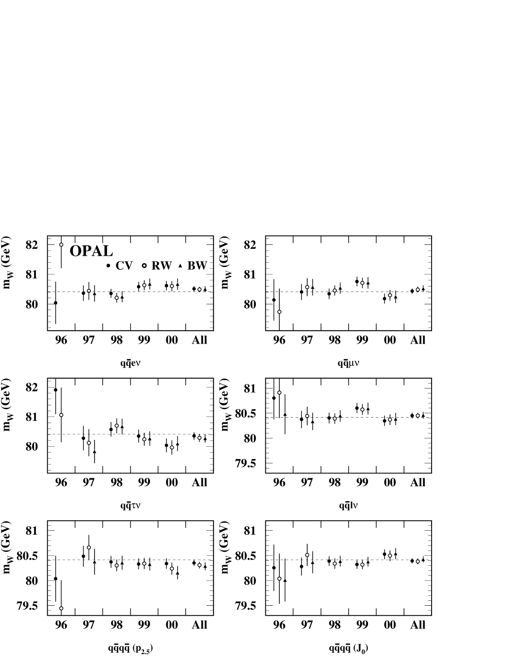
Figure 4: W mass results (with statistical errors only) for each channel in the convolution (CV), reweighting (RW) and Breit-Wigner (BW) fitting methods, as a function of data-taking year, and for all years combined. Results are shown for the $\rm q\bar{q}e\nu$, $\rm q\bar{q}\mu\nu$, $\rm q\bar{q}\tau\nu$ and combined $\rm q\bar{q}\ell\nu$ channels, and for the $\rm q\bar{q}q\bar{q}$ channel with the modified ($p_{2.5}$) and $J_{0}$ jet direction reconstruction methods. The results for the Breit-Wigner $\rm q\bar{q}\ell\nu$ and $\rm q\bar{q}q\bar{q}$ fits to 1996 data are taken from [5]. The dotted line indicates the central measured value of $m_{\rm W}$ from the present paper.

The corresponding results for the width are shown in Table 3 and Figure 5. The 1996 data at $\mbox{$\sqrt{s}$}\approx 172$ GeV are not used for the width analysis. Again, the statistical uncertainties are compatible with expectations, and the individual year results are consistent, the $\chi^{2}$ values being 5.4 and 2.1 for the $\rm q\bar{q}\ell\nu$ and $\rm q\bar{q}q\bar{q}$ channels, each for three degrees of freedom. The statistical correlation between the $\rm q\bar{q}\ell\nu$ mass and width results is estimated using Monte Carlo subsamples to be $-0.19$, whereas that for the $\rm q\bar{q}q\bar{q}$ channel results is found to be negligible. Note that the $\rm q\bar{q}q\bar{q}$ width analysis is performed using the unmodified $J_{0}$ jet direction reconstruction as this gives the optimal balance between statistical and systematic errors from hadronisation and final-state interactions, and minimises the total error. The width result from the CV5 convolution fit in the $\rm q\bar{q}\ell\nu$ channel is also shown; this fit also measures the W mass and gives a result of $80.424\pm 0.077$ GeV, consistent with that derived from the standard convolution fit. The statistical correlation coefficient between the CV5 width and mass fit results is 0.28.

	Convolution		Reweighting		CV5 convolution
Channel	Fitted $\Gamma_{\rm W}$	$\sigma_{\rm exp}$	Fitted $\Gamma_{\rm W}$	$\sigma_{\rm exp}$	Fitted $\Gamma_{\rm W}$	$\sigma_{\rm exp}$
	(GeV)	(GeV)	(GeV)	(GeV)	(GeV)	(GeV)
$\rm q\bar{q}e\nu$	$1.696\pm 0.202$	0.204	$2.009\pm 0.200$	0.202	$1.975\pm 0.230$	0.224
$\rm q\bar{q}\mu\nu$	$2.181\pm 0.233$	0.216	$2.146\pm 0.224$	0.227	$2.138\pm 0.233$	0.218
$\rm q\bar{q}\tau\nu$	$1.763\pm 0.289$	0.289	$2.089\pm 0.276$	0.309	$2.204\pm 0.188$	0.241
$\rm q\bar{q}\ell\nu$	$1.926\pm 0.135$	0.134	$2.088\pm 0.131$	0.127	$2.103\pm 0.120$	0.131
$\rm q\bar{q}q\bar{q}$ ($J_{0}$)	$2.125\pm 0.111$	0.114	$2.176\pm 0.129$	0.134	—	—

Table 3: W width results (with statistical errors only) for each channel and fitting method. The expected statistical errors $\sigma_{\rm exp}$ from Monte Carlo subsample tests are also given. The Breit-Wigner fit does not measure the W width.

Figure 5: W width results (with statistical errors only) for each channel in the convolution (CV), reweighting (RW) and 5C convolution (CV5) fitting methods, as a function of data-taking year, and for all years combined. Results are shown for the $\rm q\bar{q}e\nu$, $\rm q\bar{q}\mu\nu$, $\rm q\bar{q}\tau\nu$ and combined $\rm q\bar{q}\ell\nu$ channels, and for the $\rm q\bar{q}q\bar{q}$ channel with the $J_{0}$ jet algorithm. Only the reweighting fit measures the W width using the 1996 data, where results are shown for the $\rm q\bar{q}\ell\nu$ and $\rm q\bar{q}q\bar{q}$ channels only. The dotted line indicates the central measured value of $\Gamma_{\rm W}$ from the present paper.

In order to study the evolution of the fitted W mass with changing jet direction reconstruction, the complete convolution fit has been repeated fifteen times, using momentum cuts at 1.0, 1.75, 2.0, 2.5, 3.0 and 4.0 GeV (2.5 GeV being used for the $\rm q\bar{q}q\bar{q}$ analysis result in this paper), momentum weights $p^{\kappa}$ with $\kappa$ values of 0.5, 0.75, 1.0, $-0.5$ and $-0.75$, and cones of half-angle $R=$0.3, 0.4, 0.5 and 0.6 rad. For each jet direction reconstruction method, the mass difference with respect to the $J_{0}$ direction reconstruction using all particles associated to the jet $\mbox{$\Delta m(J_{X},J_{0})$}=m(X)-m(J_{0})$ is calculated in both the $\rm q\bar{q}\ell\nu$ and $\rm q\bar{q}q\bar{q}$ channels. The statistical error on $\Delta m(J_{X},J_{0})$ is also calculated, using Monte Carlo subsamples to take into account the correlation due to the different reconstruction methods being applied to the same events. The results are shown in Figure 6. The $\rm q\bar{q}\ell\nu$ $\Delta m(J_{X},J_{0})$ values are generally slightly positive, but the changes in fitted W mass are consistent with the expected level of statistical fluctuations, demonstrating that the $\rm q\bar{q}\ell\nu$ W mass results are stable with respect to changing the jet direction reconstruction over all methods and a wide range of parameter values. The $\rm q\bar{q}q\bar{q}$ $\Delta m(J_{X},J_{0})$ results also tend to be close to zero, with the exception of the result from jet direction reconstruction $\kappa_{-0.5}$ (with enhanced sensitivity to low momentum particles), which is significantly higher ($\mbox{$\Delta m(\mbox{$\kappa_{-0.5}$},J_{0})$}=114\pm 47$ MeV) than the results with all other jet direction definitions. The result from method $\kappa_{-0.75}$ also shows a high value of $\Delta m(\mbox{$\kappa_{-0.75}$},J_{0})$, although with low significance. Note that hadronisation uncertainties are also significant in these comparisons, and increase to around 20 MeV for the alternative jet direction reconstruction methods, as discussed in Section 8.2.

Sensitivity to final-state interactions in the $\rm q\bar{q}q\bar{q}$ channel can be maximised by studying the variable

$$\mbox{$\Delta m(J_{X},\mbox{$\kappa_{-0.5}$})$}=m(X)-m(\mbox{$\kappa_{-0.5}$})\,,$$ (9)

the difference in W mass between jet direction reconstruction methods with reduced and increased sensitivity to these effects. The largest deviation from zero is seen for $\mbox{$\Delta m(\mbox{$p_{2.5}$},\mbox{$\kappa_{-0.5}$})$}=-152\pm 68$ MeV, where the error is purely statistical, but takes into account correlations between the different reconstruction methods. The use of the mass differences to place limits on the effect of final-state interactions, specifically colour reconnection, is discussed in Section 9.1.

Figure 6: Differences in $m_{\rm W}$ measured using various jet direction reconstruction methods $X$ and the $J_{0}$ reconstruction method, for both $\rm q\bar{q}\ell\nu$ and $\rm q\bar{q}q\bar{q}$ data in the convolution fit. The points are highly correlated; the errors are purely statistical and take into account the correlation between the result from each alternative direction reconstruction method and that from $J_{0}$.

6 The reweighting fit

The reweighting fit extracts the W mass and width by comparing reconstructed data distributions with Monte Carlo ‘template’ distributions with varying $m_{\rm W}$ and $\Gamma_{\rm W}$. Templates of arbitrary $m_{\rm W}$ and $\Gamma_{\rm W}$ are obtained by reweighting Monte Carlo simulated data samples containing all signal and background final states, and a maximum likelihood fit is used to find the values of $m_{\rm W}$ and $\Gamma_{\rm W}$ that best describe the data. The reweighting fit is a more sophisticated development of that used in [7], the main changes being the use of simultaneous reweighting in three ($\rm q\bar{q}e\nu$, $\rm q\bar{q}\mu\nu$ and $\rm q\bar{q}q\bar{q}$) or two ($\rm q\bar{q}\tau\nu$) reconstructed variables, and an improved procedure for handling the combinatorial background in the $\rm q\bar{q}q\bar{q}$ channel.

In more detail, the likelihood for each event $i$ is given by

$${\cal{L}}^{\rm evt}_{i}(\mbox{$\vec{\alpha}$}_{i}|\mbox{$m_{\rm W}$},\mbox{$\Gamma_{\rm W}$})={\cal{P}}^{\rm sig}{\cal{L}}^{\rm sig}(\mbox{$\vec{\alpha}$}_{i}|\mbox{$m_{\rm W}$},\mbox{$\Gamma_{\rm W}$})+{\cal{P}}^{\rm ZZ}{\cal{L}}^{\rm ZZ}(\mbox{$\vec{\alpha}$}_{i})+{\cal{P}}^{\rm Z/\gamma}{\cal{L}}^{\rm Z/\gamma}(\mbox{$\vec{\alpha}$}_{i})\,,$$ (10)

where $\vec{\alpha}$ is the set of reconstructed variables used in the likelihood, ${\cal{L}}^{\rm sig}(\mbox{$\vec{\alpha}$}|\mbox{$m_{\rm W}$},\mbox{$\Gamma_{\rm W}$})$, ${\cal{L}}^{\rm ZZ}(\mbox{$\vec{\alpha}$})$ and ${\cal{L}}^{\rm Z/\gamma}(\mbox{$\vec{\alpha}$})$ are the likelihood distributions of the variables $\vec{\alpha}$ in WW, $\rm ZZ$ and $\mbox{$\rm Z$}/\gamma$ events, and ${\cal{P}}^{\rm sig}$, ${\cal{P}}^{\rm ZZ}$ and ${\cal{P}}^{\rm Z/\gamma}$ are the (fixed) fractions of WW, ZZ and $\mbox{$\rm Z$}/\gamma$ events in the sample, estimated from Monte Carlo simulation at the corresponding centre-of-mass energy. The signal probability distribution ${\cal{L}}^{\rm sig}(\mbox{$\vec{\alpha}$}|\mbox{$m_{\rm W}$},\mbox{$\Gamma_{\rm W}$})$ is obtained by reweighting four-fermion Monte Carlo events with a true W mass of $\mbox{$m^{0}_{\rm W}$}=80.33$ GeV and a width of $\mbox{$\Gamma^{0}_{\rm W}$}=2.09$ GeV by the ratio of two Breit-Wigner functions. The weight $f_{i}$ for a Monte Carlo event $i$ with true event-by-event W boson masses $m^{\prime}_{1}$ and $m^{\prime}_{2}$ is given by

$$f_{i}=\frac{B(\mbox{$m^{\prime}_{1}$}|\mbox{$m_{\rm W}$},\mbox{$\Gamma_{\rm W}$})\ B(\mbox{$m^{\prime}_{2}$}|\mbox{$m_{\rm W}$},\mbox{$\Gamma_{\rm W}$})}{B(\mbox{$m^{\prime}_{1}$}|\mbox{$m^{0}_{\rm W}$},\mbox{$\Gamma^{0}_{\rm W}$})\ B(\mbox{$m^{\prime}_{2}$}|\mbox{$m^{0}_{\rm W}$},\mbox{$\Gamma^{0}_{\rm W}$})}$$ (11)

where the Breit-Wigner function $B(m|\mbox{$m_{\rm W}$},\mbox{$\Gamma_{\rm W}$})$ is given by Equation 2. The effect of background is accounted for via the background terms in Equation 10, whose probability distributions are calculated as a function of $\vec{\alpha}$ using large samples of unweighted background Monte Carlo events.

The probability distributions ${\cal{L}}^{\rm sig}$, ${\cal{L}}^{\rm ZZ}$ and ${\cal{L}}^{\rm Z/\gamma}$ are calculated in bins of the reweighting fit variables $\vec{\alpha}$, the bin size varying with $\vec{\alpha}$ in order to achieve an approximately constant number of events per bin and minimise fluctuations from limited Monte Carlo statistics. The likelihood for the whole sample is therefore obtained from the number of events $N_{j}$ in each bin $j$ where the variables take the values $\mbox{$\vec{\alpha}$}_{j}$:

$${\cal{L}}^{\rm tot}(\mbox{$m_{\rm W}$},\mbox{$\Gamma_{\rm W}$})=\prod_{j}\left[\left({\cal{L}}^{\rm evt}(\mbox{$\vec{\alpha}$}_{j}|\mbox{$m_{\rm W}$},\mbox{$\Gamma_{\rm W}$})\right)^{N_{j}}\right]$$ (12)

Two types of reweighting fit are performed. In the first, the likelihood ${\cal{L}}^{\rm tot}$ is maximised as $m_{\rm W}$ is varied and $\Gamma_{\rm W}$ is determined from $m_{\rm W}$  by the Standard Model relation (Equation 7). In the second, a two parameter fit is performed, allowing both $m_{\rm W}$ and $\Gamma_{\rm W}$ to vary simultaneously. The results for $m_{\rm W}$ are very similar in both cases, but for consistency with the convolution and Breit-Wigner analyses, the result of the first fit is used for the reweighting fit W-mass result in this paper.

6.1 The ${\rm\bf q\bar{q}}\ell\nu$ reweighting fit

The $\rm q\bar{q}\ell\nu$ reweighting fit uses the same basic event selection as the convolution fit. In the $\rm q\bar{q}e\nu$ and $\rm q\bar{q}\mu\nu$ channels, both 4C and 5C kinematic fits are performed, and all events for which both kinematic fits converge are retained. The reweighting fit is performed simultaneously in three reconstructed variables which make up the variable set $\vec{\alpha}$:

• The reconstructed W mass from the 5C fit, $m_{\rm 5C}$, in 16 bins from 65 to 105 GeV.

• The error on the reconstructed 5C fit mass, $\sigma_{m_{\rm 5C}}$, in five bins from 0.5 to 6.5 GeV.

• The two-jet invariant mass from the 4C fit, in four bins from 40 to 140 GeV.

The bin sizes vary, and are chosen such that each of the 320 bins in each channel is populated by about 400 Monte Carlo events. Events are discarded if any of the variables fall outside the bin ranges. The use of the error on the 5C fit mass and the jet-jet invariant mass significantly improves the statistical precision of the fit as compared to the one-dimensional reweighting using $m_{\rm 5C}$ alone [7].

In the $\rm q\bar{q}\tau\nu$ channel, all information comes from the hadronic system and is extracted using an analytic implementation of the 5C fit. Two variables are used, namely the 5C fit mass (20 bins from 65 to 105 GeV) and its error (five bins from 0 to 6.5 GeV). A variable bin size is again used, with around 1000 Monte Carlo events per bin. Events with a kinematic fit probability of less than $10^{-3}$ are removed.

The reweighting fit technique should implicitly correct for all effects which bias the reconstructed W mass, providing they are included in the Monte Carlo simulation used to generate the template distributions. Therefore, the effects of initial-state radiation, event selection and reconstruction biases are all included. This is checked using large Monte Carlo samples over the full range of centre-of-mass energies and true W masses from 79.33–81.33 GeV. The errors returned by the fits are similarly checked by studying the pull distributions in Monte Carlo subsamples, and found to be unbiased.

6.2 The $\rm\bf q\bar{q}q\bar{q}$ reweighting fit

The $\rm q\bar{q}q\bar{q}$ reweighting fit uses the same basic event selection as the convolution fit. However, the method used for the assignment of jets to the two W bosons is rather different, with only one combination per event entering the final fit. The tracks and clusters of the event are first grouped into five jets using the Durham jet algorithm, and a 4C kinematic fit is performed. The value of the variable $\bar{y}_{ij}=E_{i}E_{j}(1-\cos\theta_{ij})$ calculated for each pair of jets, where $E_{i}$ and $E_{j}$ are the fitted energies of jets $i$ and $j$ and $\theta_{ij}$ is the angle between them. The five fitted jets are assigned to the two W bosons requiring that the pair of jets with the lowest $\bar{y}_{ij}$ is always kept together, both jets being assigned to the same W boson. Each of the other three jets is then assigned in turn to the same W boson as the paired jets. This results in three distinct jet assignment combinations, which are each fitted with a 5C kinematic fit.

In the $\rm q\bar{q}q\bar{q}$ analysis with the $p_{2.5}$ jet direction reconstruction method, the best of the three jet combinations is determined using the jet-pairing likelihood technique described in [7], with the two jets corresponding to the minimum $\bar{y}_{ij}$ merged into a single jet. For each of the possible jet pairing assignments, three input variables are calculated and fed into a likelihood discriminant, and the combination with the largest output value is retained for the fit. The likelihood reference distributions are determined using large Monte Carlo samples, separately at each centre-of-mass energy. The input variables consist of the value of the CC03 matrix element for W-pair production [25], determined from the measured four-vectors of the reconstructed jets; the difference in reconstructed masses of the two W bosons, determined using the initial 4C kinematic fit; and the sum of the di-jet opening angles. The CC03 matrix element is averaged over three assumed W mass values from 80.1 to 80.6 GeV. This algorithm selects a jet assignment combination in every selected $\rm q\bar{q}q\bar{q}$ event, and is correct 72 % of the time. For the $\rm q\bar{q}q\bar{q}$ analysis with the $J_{0}$ jet algorithm, the jet angular resolution is such that the CC03 matrix element provides good discriminating power by itself, and the jet-pairing likelihood is not used. This algorithm selects the correct jet assignment in 74 % of cases.

Having selected one jet assignment combination, the corresponding 4C and 5C kinematic fits are used to provide the reconstructed variables entering the reweighting fit likelihood. These variables are:

• The reconstructed W mass from the 5C fit, $m_{\rm 5C}$, in 24 bins from 65 to 105 GeV.

• The error on the 5C fit mass, $\sigma_{m_{\rm 5C}}$, in 5 bins from zero to 5 GeV.

• The difference of the two 4C fit masses, $\delta m$, in 5 bins from $-50$ to 55 GeV. The mass difference is signed such that the W boson containing the jet with the highest energy before the kinematic fit contributes with a positive sign.

As for the $\rm q\bar{q}\ell\nu$ fit, the bin sizes are chosen so that each bin is populated by around 400 Monte Carlo events. Events in which either of the fits fail, or in which any of the reconstructed variables fall outside the given range, are discarded.

The fit method is checked using large Monte Carlo samples as for the $\rm q\bar{q}\ell\nu$ reweighting fit. The errors returned by the fit are also checked by studying pull distributions in Monte Carlo subsample tests, and found to be unbiased.

6.3 Reweighting fit results

The reweighting fit is used to analyse the data from each year and channel separately, and the results for the different years are combined to give the values shown in Tables 2 and 3. The results from each year are also shown separately as the ‘RW’ points in Figures 4 and 5. As discussed above the mass values are determined using a one parameter fit to $m_{\rm W}$ only, and the width values are determined using a two parameter fit to $m_{\rm W}$ and $\Gamma_{\rm W}$. In the latter fits, the correlation coefficients between $m_{\rm W}$ and $\Gamma_{\rm W}$ are $0.08$ in the $\rm q\bar{q}\ell\nu$ channel and $0.07$ in the $\rm q\bar{q}q\bar{q}$ channel, and the mass results agree with those from the one parameter fits to within 1 MeV. No separate $\Gamma_{\rm W}$ results are shown for the individual $\rm q\bar{q}e\nu$, $\rm q\bar{q}\mu\nu$ and $\rm q\bar{q}\tau\nu$ channels in 1996 due to the small numbers of selected events, but the 1996 data are included in the overall averages. The expected statistical errors are also given in Tables 2 and 3, evaluated using Monte Carlo subsample tests. The statistical errors on the data results are again consistent with those expected from Monte Carlo, taking into account the expected level of statistical fluctuations.

The reconstructed mass distributions from the 5C fits can be seen in Figures 7(a) and (b), for both the $\rm q\bar{q}\ell\nu$ and $\rm q\bar{q}q\bar{q}$ channels (for the latter only the selected jet assignment combinations are shown). The reweighted Monte Carlo template distributions corresponding to the fitted values of $m_{\rm W}$ in each channel are also shown, including both signal (WW events with the correct jet assignment) and background contributions. The width of the $\rm q\bar{q}\ell\nu$ mass peak is smaller than that from the convolution fit shown in Figure 2 because the latter displays the average of the two fitted W masses in each event. This average does not take into account the better resolution of the $\rm q\bar{q}$ system mass compared to that of the $\ell\nu$ system, information which is however included in the convolution fit itself.

Figure 7: Distributions of 5C fit masses for the $\rm q\bar{q}\ell\nu$ and $\rm q\bar{q}q\bar{q}$ channels in the reweighting (a,b) and Breit-Wigner (c,d) fits. For the reweighting fits, the histograms show the reweighted template distributions corresponding to the fitted W mass values, and for the Breit-Wigner fits, the fitted functions are indicated by the solid lines drawn over the fit regions (70–88 GeV). In both cases, the estimated background contributions are indicated by the shaded regions.

7 The Breit-Wigner fit

The Breit-Wigner fit is based on a simple likelihood fit to the distribution of W boson masses reconstructed using a 5C kinematic fit in each event, and is very similar to that described in [5]. The main motivation for this analysis is to extract the W mass using a simple and transparent method, to act as a cross-check for the convolution and reweighting fits. The Breit-Wigner fit does not measure the W width.

The event selection and reconstruction are very similar to those of the convolution and reweighting fits. In the $\rm q\bar{q}\ell\nu$ channel, only events with a 5C kinematic fit probability exceeding $10^{-3}$ are used in the analysis. Events in each of the lepton sub-channels ($\rm q\bar{q}e\nu$, $\rm q\bar{q}\mu\nu$ and $\rm q\bar{q}\tau\nu$) are treated separately, and the $\rm q\bar{q}\tau\nu$ channel is further divided into events where the $\tau$ decays leptonically or hadronically. In the $\rm q\bar{q}q\bar{q}$ channel, events are reconstructed as five jets if the Durham jet resolution parameter $y_{45}>0.0037$ (about 23 % of the events), and as four jets otherwise. In four-jet events, 5C kinematic fits are performed on all three possible jet pairings. The fit with the highest probability $P_{1}$ is used if $P_{1}>0.003$ for the $p_{2.5}$ jet direction reconstruction method, and $P_{1}>0.01$ for the $J_{0}$ method. The fit with the second-highest probability $P_{2}$ is also used (with equal weight) if it passes both the previous probability cut and $P_{2}>\frac{1}{3}P_{1}$; this occurs in approximately 20 % of events. In five-jet events, at most one of the possible ten jet assignment combinations is used, selected according to the output of the jet assignment likelihood algorithm used in [7]. The likelihood inputs are the difference between the two W masses in a 4C fit, the largest inter-jet opening angle between jets in the three-jet system, and the cosine of the polar angle of the three-jet system. The jet combination giving the largest likelihood value is used provided the value is greater than a minimum cut requirement, which happens in 73 % of selected five-jet WW events.

In all channels, the fitted W mass value is extracted using an unbinned maximum likelihood fit to the distribution of reconstructed 5C fit masses $m$ in the region $70<m<88$ GeV. The fit function is chosen empirically and consists of two terms: $S(m)$ describes the signal contribution and $B(m)$ the combinatorial and non-WW background. In the $\rm q\bar{q}\ell\nu$ channel, the signal function consists of an asymmetric relativistic Breit-Wigner function with different widths above and below the peak:

$$S(m)=A\frac{m^{2}\Gamma^{2}_{1,2}}{(m^{2}-m_{0}^{2})^{2}+m^{2}\Gamma^{2}_{1,2}}\,,$$ (13)

where $m_{0}$ is the fitted mass and $\Gamma_{1,2}$ are fixed parameters, $\Gamma_{1}$ being taken for $m<m_{0}$ and $\Gamma_{2}$ otherwise, and $A$ is a normalisation constant. In the $\rm q\bar{q}q\bar{q}$ channel the signal function $S(m)$ is additionally multiplied by a Gaussian function of mean $m_{0}$ and width $\sigma$, since this is found to improve the description of the reconstructed 5C fit mass distribution. These parameterisations were found to give adequate descriptions of the reconstructed distributions in Monte Carlo simulated data samples of around ten times the data luminosity. The parameters $\Gamma_{1}$ and $\Gamma_{2}$ were determined using large samples of Monte Carlo signal events with $\mbox{$m_{\rm W}$}=80.33$ GeV, and were parameterised as linear functions of $\sqrt{s}$. The parameter $\sigma$ for the $\rm q\bar{q}q\bar{q}$ channel was similarly determined and found to be independent of $\sqrt{s}$.

The contributions from combinatorial WW background, ZZ and $\mbox{$\rm Z$}/\gamma$ final states are represented by the background function $B(m)$, derived from Monte Carlo simulated events separately at each centre-of-mass energy. The fractions of background assumed in the fits are fixed to those observed in Monte Carlo. As for the convolution fit, the fitted mass $m_{0}$ must be corrected for biases arising from initial-state radiation, the event selection, reconstruction and fitting procedures. Studies using Monte Carlo samples with the full range of $\sqrt{s}$ values and true W masses from 79.33–81.33 GeV show these biases to have magnitudes of up to 500 MeV (in the $\rm q\bar{q}\tau\nu$ and $\rm q\bar{q}q\bar{q}$ channels), to be independent of $\sqrt{s}$, but to depend slightly on the true W mass. They were therefore parameterised as linear functions of the fitted mass using large Monte Carlo samples of both signal and background events, and applied as corrections to the raw fitted mass values.

The Breit-Wigner fit is applied separately to the data taken at each centre-of-mass energy from 183 GeV to 209 GeV (dividing the 1999 and 2000 data samples into four and two energy bins respectively), and the results combined. The results for each channel (including both the modified $p_{2.5}$ and $J_{0}$ jet direction reconstruction methods in the $\rm q\bar{q}q\bar{q}$ channel) are shown in Table 2, together with the expected statistical errors evaluated using Monte Carlo subsample tests. The results are also shown as a function of data-taking year as the ‘BW’ points in Figure 4. Data taken in 1996 at $\mbox{$\sqrt{s}$}\approx 172\,$GeV have not been reanalysed, and the Breit-Wigner fit results from [5] are shown. The reconstructed 5C mass distributions for $\rm q\bar{q}\ell\nu$ events and selected jet assignment combinations in $\rm q\bar{q}q\bar{q}$ events are shown in Figure 7(c) and (d), together with the fitted functions used to extract the W mass.

8 Systematic uncertainties

The main systematic uncertainties in the measurements of the W mass and width arise from the understanding of the detector calibration and performance, the hadronisation of quarks into jets, possible final-state interactions in the $\rm q\bar{q}q\bar{q}$ channel, the modelling of non-WW background, the simulation of photon radiation in WW events and uncertainties in the LEP beam energy. These and other small systematic effects have been calculated separately for the $\rm q\bar{q}\ell\nu$ and $\rm q\bar{q}q\bar{q}$ channels, using all three analysis techniques for the W mass, and for the convolution and reweighting fits for the W width. The determination of all systematic errors is described in detail below, and the results are summarised in Tables 4 and 5. Detector-related effects tend to increase slightly with energy; other uncertainties are taken to be constant unless stated otherwise. The magnitudes of the systematic uncertainties are generally rather similar between the different fitting techniques, but there are some significant differences, and these are also discussed below.

	$\rm q\bar{q}\ell\nu$			$\rm q\bar{q}q\bar{q}$			$\rm q\bar{q}q\bar{q}$		Comb.	$\rm q\bar{q}q\bar{q}$
				$p_{2.5}$			$J_{0}$	$\kappa_{-0.5}$		$\Delta m$
Source	CV	RW	BW	CV	RW	BW	CV	CV	CV	CV
Jet energy scale	7	1	2	4	4	4	5	4	6	0
Jet energy resolution	1	1	1	0	1	3	1	0	0	0
Jet energy linearity	9	9	12	2	2	4	2	1	6	1
Jet angular resolution	0	0	0	0	0	0	0	0	0	1
Jet angular bias	4	4	4	7	7	6	6	7	5	1
Jet mass scale	10	7	6	5	11	3	5	5	8	0
Electron energy scale	9	6	8	-	-	-	-	-	6	-
Electron energy resolution	2	2	6	-	-	-	-	-	1	-
Electron energy linearity	1	1	2	-	-	-	-	-	1	-
Electron angular resolution	0	0	0	-	-	-	-	-	0	-
Muon energy scale	8	7	7	-	-	-	-	-	6	-
Muon energy resolution	2	2	3	-	-	-	-	-	1	-
Muon energy linearity	2	2	2	-	-	-	-	-	1	-
Muon angular resolution	0	0	0	-	-	-	-	-	0	-
WW event hadronisation	14	8	16	20	26	18	6	19	16	40
Colour reconnection	-	-	-	41	41	32	125	228	14	-
Bose-Einstein correlations	-	-	-	19	18	21	35	64	6	45
Photon radiation	11	11	10	9	8	8	9	9	10	0
Background hadronisation	2	1	2	20	12	32	17	24	8	4
Background rates	1	0	5	6	2	7	4	7	3	0
LEP beam energy	8	9	9	10	11	10	10	10	9	-
Modelling discrepancies	4	0	0	15	0	0	10	11	8	5
Monte Carlo statistics	2	3	3	2	3	3	2	2	2	3
Total systematic error	28	22	29	58	56	56	133	240	32	61
Statistical error	56	58	64	60	64	73	51	73	42	68
Total error	63	62	70	83	85	92	142	251	53	91

Table 4: Summary of systematic uncertainties (in MeV) on the measurements of the W mass. Results are given separately for the $\rm q\bar{q}\ell\nu$ and $\rm q\bar{q}q\bar{q}$ channels ($p_{2.5}$ jet direction reconstruction) with the convolution, reweighting and Breit-Wigner fitting methods. Results are also given for the convolution fit for the $J_{0}$ and $\kappa_{-0.5}$ jet direction reconstruction methods, and for the combination of convolution $\rm q\bar{q}\ell\nu$ and $\rm q\bar{q}q\bar{q}$ ($p_{2.5}$) results (where the combination takes the systematic uncertainties and their correlations into account). The last column gives the systematic uncertainties for the mass difference $\Delta m(\mbox{$p_{2.5}$},\mbox{$\kappa_{-0.5}$})$ discussed in Section 9.1.

	$\rm q\bar{q}\ell\nu$		$\rm q\bar{q}q\bar{q}$		Comb.
Source	CV	RW	CV	RW	CV
Jet energy scale	0	7	0	2	0
Jet energy resolution	16	12	4	5	12
Jet energy linearity	6	1	1	1	4
Jet angular resolution	2	3	4	3	2
Jet angular bias	2	2	0	3	1
Jet mass scale	6	2	1	7	4
Electron energy scale	7	2	-	-	4
Electron energy resolution	27	40	-	-	18
Electron energy linearity	0	0	-	-	0
Electron angular resolution	1	0	-	-	1
Muon energy scale	7	5	-	-	4
Muon energy resolution	8	20	-	-	5
Muon energy linearity	1	1	-	-	0
Muon angular resolution	0	0	-	-	0
WW event hadronisation	77	55	68	98	74
Colour reconnection	-	-	151	136	53
Bose-Einstein correlations	-	-	32	13	11
Photon radiation	11	34	10	26	11
Background hadronisation	10	10	32	46	18
Background rates	18	20	34	32	24
LEP beam energy	3	1	2	1	3
Modelling discrepancies	4	0	25	0	11
Mass-width coupling	24	0	0	0	16
Monte Carlo statistics	9	12	8	12	9
Total systematic error	91	85	177	180	102
Statistical error	135	131	112	130	96
Total error	163	156	209	222	140

Table 5: Summary of systematic uncertainties (in MeV) on the measurements of the W width. Results are given separately for the $\rm q\bar{q}\ell\nu$ and $\rm q\bar{q}q\bar{q}$ channels with the convolution and reweighting fitting methods. The systematic uncertainties for the combination of $\rm q\bar{q}\ell\nu$ and $\rm q\bar{q}q\bar{q}$ convolution fit results are also shown.

8.1 Detector calibration and simulation

The Monte Carlo descriptions of the jet and lepton energy scales, and energy and angular resolutions, are checked using samples of $\mbox{$\rm Z$}\rightarrow\mbox{$\rm q\bar{q}$}$, $\mbox{$\rm Z$}\rightarrow\mbox{$\rm e^{+}e^{-}$}$ and $\mbox{$\rm Z$}\rightarrow\mbox{$\mu^{+}\mu^{-}$}$ events recorded at $\mbox{$\sqrt{s}$}\approx 91$ GeV at the beginning of each data-taking year, and at other times during the data-taking periods in 1998, 1999 and 2000. Detailed comparisons between these data and corresponding Monte Carlo simulations are used to derive small adjustments at the level of reconstructed jets and leptons, which are then applied to the WW and background samples that are used to calibrate the bias corrections in the convolution and Breit-Wigner fits and to derive template distributions in the reweighting fit. Where necessary, the energy and angular resolution in the Monte Carlo simulation are degraded by applying Gaussian smearing to the reconstructed quantities. The associated systematic uncertainties are propagated to the measured W mass and width by varying the applied corrections.

The properties of jets are checked using samples of two-jet and three-jet $\mbox{$\rm Z$}\rightarrow\mbox{$\rm q\bar{q}$}$ events, and $\mbox{$\mbox{$\rm Z$}/\gamma$}\rightarrow\mbox{$\rm q\bar{q}$}$ events from the high-energy LEP2 data samples, as follows:

Jet energy scale:

This is checked using $\mbox{$\rm Z$}\rightarrow\mbox{$\rm q\bar{q}$}$ events reconstructed as two jets with the Durham algorithm and satisfying $y_{23}<0.02$. The same particle selection requirements and energy double-counting correction procedure are applied as for the WW analysis. The mean of the sum of the two jet energies is studied as a function of $\cos\theta=\frac{1}{2}(|\cos\theta_{1}|+|\cos\theta_{2}|)$, where $\theta_{1}$ and $\theta_{2}$ are the reconstructed polar angles of the two jets. The ratio of these energy sums in data and Monte Carlo is shown in Figure 8(a), and is used to derive corrections to the Monte Carlo energy scale as functions of jet $\cos\theta$ and data-taking year. The corrections in the forward region beyond $\cos\theta=0.85$ are much larger than in the central region, due to the difficulties in accurately modelling the complex detector geometry and larger amount of dead material. The residual uncertainty on the jet energy scale is 0.4 %, dominated by contributions from $\rm Z$ data statistics, possible quark-flavour dependences (assessed by repeating the studies after removing events with a reconstructed secondary vertex indicating a heavy quark decay [28]) and possible variations during the course of a year.

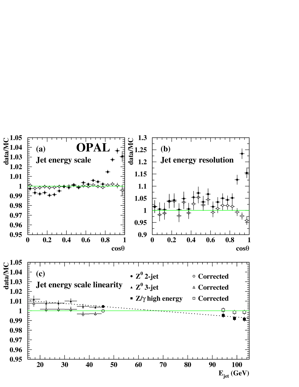
Figure 8: Determination of energy corrections for jets (see text). Ratios of data to Monte Carlo are shown averaged over all data-taking years for: (a) jet energy scale as a function of $\cos\theta$, (b) jet energy resolution as a function of $\cos\theta$, (c) jet energy scale as a function of the jet energy itself. The results using the uncorrected simulation are shown by the filled points, and those with the corrected simulation are shown by the open points, with the error bars indicating the statistical error in each case. The horizontal lines indicate ratios of unity, and the dotted line in (c) shows the linearity correction used to parameterise the jet energy scale dependence on the jet energy itself.

Jet energy resolution:

The width of the distribution of two-jet energy sums is sensitive to the jet energy resolution, and was studied using the same techniques as the energy scale. The ratio of widths seen in data and Monte Carlo is shown in Figure 8(b)—the Monte Carlo resolution is about 4 % too good for $\cos\theta<0.85$, and up to 20 % too good in the forward region beyond $\cos\theta=0.85$. After correction, the residual uncertainty lies between 0.6 % and 2 % depending on $\cos\theta$, limited by $\rm Z$ data statistics.

Jet energy linearity:

The studies with two-jet $\mbox{$\rm Z$}\rightarrow\mbox{$\rm q\bar{q}$}$ events check the energy scale for $\sim 45$ GeV jets, close to the average energy of jets produced in W decays, but event-by-event the latter range from about 20 GeV to 85 GeV. It is therefore important to check the linearity of the energy response, i.e. the energy scale for lower and higher energy jets. This has been studied by looking both at $\mbox{$\rm Z$}\rightarrow\mbox{$\rm q\bar{q}$}\rm g$ three-jet events and high energy $\mbox{$\mbox{$\rm Z$}/\gamma$}\rightarrow\mbox{$\rm q\bar{q}$}$ two-jet events. Coplanar three-jet events are selected by requiring $y_{23}>0.02$ and $y_{34}<0.005$, and that the sum of the inter-jet angles exceeds 355^∘. The jet energies can then be computed using the measured jet angles and masses, and the ratio of reconstructed to expected energies determined as a function of expected energy. The ratio of this quantity in data and Monte Carlo is shown in Figure 8(c), from which it can be seen that the energy scale in data is around 0.5 % higher for 30 GeV jets than for 45 GeV jets.

The behaviour at high jet energies is studied with $\mbox{$\mbox{$\rm Z$}/\gamma$}\rightarrow\mbox{$\rm q\bar{q}$}$ events taken at $\mbox{$\sqrt{s}$}>180\,$GeV, and satisfying $y_{23}<0.02$ and $\sqrt{s^{\prime}/s}>0.85$ where the reconstructed $\rm e^{+}e^{-}$ collision energy after any initial-state radiation $\sqrt{s^{\prime}}$ is calculated as in [9]. In these events, the behaviour of the jet energy scale as a function of $\cos\theta$ is consistent with that seen for 45 GeV jets, but the overall energy scale is shifted downwards by about 1 %, as can be seen for the high jet energy points in Figure 8(c).

These studies are consistent with a linear dependence of the jet energy scale on the jet energy itself, with a slope of $(-2.00\pm 0.30)\times 10^{-4}$. The corresponding correction is applied to the energy scale in Monte Carlo simulation. The uncertainty is dominated by data statistics ($0.26\times 10^{-4}$), but also includes systematic contributions from two-photon ($0.06\times 10^{-4}$) and $\tau$-pair ($0.09\times 10^{-4}$) background modelling in the high energy $\rm q\bar{q}$ samples, and possible quark flavour dependences ($0.09\times 10^{-4}$). Effects from hadronisation and four-fermion background modelling are found to be negligible. This uncertainty on the correction contributes a systematic error of around 4 MeV in the $\rm q\bar{q}\ell\nu$ and 2 MeV in the $\rm q\bar{q}q\bar{q}$ W mass measurements.

Although the data are consistent with a linear slope, a second order polynomial is also fitted and used to correct the simulation as an alternative. The corresponding W mass uncertainties when the curvature is varied within the range allowed by the data are 8 MeV and 2 MeV in the $\rm q\bar{q}\ell\nu$ and $\rm q\bar{q}q\bar{q}$ channels. The final jet energy linearity uncertainties on the W mass and width are calculated as the quadrature sum of the shifts resulting from changing the linear correction by its uncertainty, and using the alternative second order polynomial correction with the maximum curvature allowed by the data.

Jet angular resolution:

The jet $\cos\theta$ and $\phi$ resolutions are checked by using the two-jet $\mbox{$\rm Z$}\rightarrow\mbox{$\rm q\bar{q}$}$ sample and studying the widths of the distributions of $\cos\theta_{1}+\cos\theta_{2}$ and $\phi_{1}-\phi_{2}$. These are found to be 4 % and 1 % narrower in Monte Carlo than data for the $J_{0}$ jet direction reconstruction method, independent of $\cos\theta$, and are smeared accordingly. The corresponding uncertainties are 0.4 % for $\cos\theta$ and 0.3 % for $\phi$, dominated by $\rm Z$ data statistics. The uncertainties for the $p_{2.5}$ direction reconstruction method are similar, though modelling of the jet angular resolution is somewhat worse. The differences between data and Monte Carlo are around a factor two larger than for the $J_{0}$ direction reconstruction, necessitating correspondingly larger Monte Carlo corrections.

Jet angular bias:

A bias in the jet $\cos\theta$ reconstruction, equal in magnitude but opposite in sign for positive and negative $\cos\theta$, would not show up in the jet acollinearity measured by $\cos\theta_{1}+\cos\theta_{2}$, and could have significant effects on the W mass and width. This is studied by using individual jets in two-jet $\mbox{$\rm Z$}\rightarrow\mbox{$\rm q\bar{q}$}$ events, and calculating their $\cos\theta$ separately using tracking and calorimeter information (the two detector systems have independent and uncorrelated angular reconstruction uncertainties). Some differences are seen, but these are generally well modelled by the Monte Carlo simulation. Since the jet $\cos\theta$ information is determined from both the tracking and calorimeter information, half the residual difference between data and Monte Carlo tracking-calorimeter deviations is taken as a systematic uncertainty on the absolute $\cos\theta$ bias. This study was performed for both the unmodified and alternative jet direction reconstruction algorithms, and no significant differences were seen.

Jet mass scale:

No useful information on jet masses can be obtained from studies of $\rm Z$ data alone, and there are significant differences between the predictions of the Jetset, Ariadne and Herwig Monte Carlo models. The jet masses predicted by the Monte Carlo are therefore left unchanged by default, and a systematic error is assessed by scaling and smearing them event-by-event by the same factor as the corresponding jet energies—this is appropriate for the extreme case of jets composed entirely of massless particles. As an additional cross-check, the energies of all particles were scaled by the same factor as the jet energies, but before calculating the jet invariant masses. This gave results which were negligibly different from those obtained by scaling the jet masses.

A similar approach is taken to study the modelling of leptons (electrons and muons separately), using $\mbox{$\rm Z$}\rightarrow\mbox{$\rm e^{+}e^{-}$}$ and $\mbox{$\rm Z$}\rightarrow\mbox{$\mu^{+}\mu^{-}$}$ events as follows:

Lepton energy scale:

The lepton energy scale is studied as a function of $\cos\theta$ using the means of distributions of lepton energies. For electrons, the ratios of data to Monte Carlo means are typically within 1 % of unity, and are used to correct the Monte Carlo simulation, with a residual systematic uncertainty of 0.3 % including contributions from possible time dependence, the comparison of two independent event selections and data statistics. The ratios of data to Monte Carlo for muons typically agree to better than 0.3 %, and a systematic uncertainty of 0.3 % is assigned, dominated by $\rm Z$ data statistics and the comparison of event selections.

Lepton energy resolution:

Studies of the width of the lepton energy distributions show that the electron energy resolution is around 19 % worse in data than Monte Carlo in the barrel region and 7 % worse in the endcap, and that the muon resolution is 6 % worse in data. These corrections are applied to the Monte Carlo with corresponding uncertainties of 2 %, dominated by data statistics. There are also tails in the data resolution which are not well modelled by the Monte Carlo. For the W mass, a systematic error is conservatively estimated by doubling the Monte Carlo resolution correction, whilst for the width (which is much more sensitive to such tails) a more elaborate two-component smearing procedure is used to model both the core and tail resolution, with an additional uncertainty relating to the choice of smearing parameters.

Lepton energy linearity:

Possible dependences of the lepton energy scale on the lepton energy itself are studied using $\mbox{$\rm e^{+}e^{-}$}\gamma$ and $\mbox{$\mu^{+}\mu^{-}$}\gamma$ events taken both during the $\rm Z$ calibration and high energy running, by comparing the measured lepton energies with those determined from the track and cluster angles. No significant effects are seen, within a statistical precision on the slope of $3\times 10^{-5}$ for electrons and $6\times 10^{-5}$ for muons, and these values are used to assess the corresponding uncertainties on the W mass and width.

Lepton angular resolution:

The lepton $\cos\theta$ and $\phi$ resolutions are studied using the distributions of $\cos\theta_{1}+\cos\theta_{2}$ and $\phi_{1}-\phi_{2}$ in the same way as discussed above for jets. No evidence for Monte Carlo mis-modelling is seen, and the corresponding uncertainties are obtained from the statistical precision of the tests of 5–10 %.

The effects of all these uncertainties on the various W mass and width analyses are shown in Tables 4 and 5. Uncertainties which affect only the $\rm q\bar{q}e\nu$ or $\rm q\bar{q}\mu\nu$ sub-channels are given in terms of their effect on the combined $\rm q\bar{q}\ell\nu$ results, and the uncertainties due to the measurements of jets and leptons are assumed to be uncorrelated. For the W mass, the most significant uncertainties are those associated with energy scales, jet angular biases and jet masses, whilst for the W width, energy resolution uncertainties play a bigger role. The uncertainties for the three fit methods are rather similar, except for the jet energy scale uncertainty in the $\rm q\bar{q}\ell\nu$ channel which is significantly smaller in the reweighting and Breit-Wigner fits than in the convolution fit. This is due to the different sensitivities of 4C and 5C kinematic fits with and without lepton information to variations of the jet energy scale, and the different use made by the three analysis methods of the different types of fit.

A further correction is applied for the effects of beam-related background and detector noise, which lead to additional non-simulated occupancy in the detectors. This correction is evaluated by superimposing data events taken with a random beam-crossing trigger onto Monte Carlo WW and background events. The most significant effects come from additional clusters in the calorimeters (especially the hadron calorimeter in the forward region), and lead to shifts of around 10 MeV in the W mass and 2 MeV in the W width, with systematic uncertainties which are negligible in comparison to other detector-related effects. The effect of this noise on the data vs. Monte Carlo comparisons discussed above was also checked and found to be negligible.

8.2 Hadronisation in $\rm\boldmath W\rightarrow\mbox{$\rm q\bar{q}$}$ decays

Uncertainties due to hadronisation in $\rm W\rightarrow\mbox{$\rm q\bar{q}$}$ decays are studied using large Monte Carlo samples where the same original four-fermion events have been hadronised using various different Monte Carlo models (string, colour dipole and cluster, as implemented in Jetset, Ariadne and Herwig respectively) and parameter sets (see Section 2). These models have all been tuned to give a reasonable overall description of OPAL or ALEPH $\mbox{$\rm Z$}\rightarrow\mbox{$\rm q\bar{q}$}$ data. Different models and tuned parameter sets describe particular features of the data to a greater or lesser extent, reflecting partly the emphasis placed on various variables (e.g. event shapes, charged and neutral particle multiplicities and fragmentation functions) by the different tune procedures.

All these models give adequate descriptions of general event properties in $\mbox{$\rm W^{+}W^{-}$}\rightarrow\mbox{$\rm q\bar{q}\ell\nu$}$ and $\mbox{$\rm W^{+}W^{-}$}\rightarrow\mbox{$\rm q\bar{q}q\bar{q}$}$ events, and the limited data statistics do not allow any of the models to be disfavoured or excluded. However, they predict different fit biases or reweighting template distributions for the W mass and width fits. This is illustrated in Table 6, which shows the biases in fitted W mass and width from the convolution fit analysis applied to the same event samples hadronised with various different models, but calibrated using Monte Carlo events hadronised using JT. The statistical errors on the mass differences are calculated using a Monte Carlo subsample technique and take into account the correlation between the samples due to the common initial four-fermion events. Taking the ‘raw’ mass shifts from Table 6, it is clear that the different models and tunes predict significantly different W mass biases, of up to $\sim 40$ MeV in both $\rm q\bar{q}\ell\nu$ and $\rm q\bar{q}q\bar{q}$ channels, and corresponding width biases of up to $\sim 80$ MeV.

Models	Raw mass shifts				Adjusted mass shifts
	$\rm q\bar{q}\ell\nu$	$\rm q\bar{q}q\bar{q}$	$\rm q\bar{q}q\bar{q}$	$\rm q\bar{q}q\bar{q}$	$\rm q\bar{q}\ell\nu$	$\rm q\bar{q}q\bar{q}$	$\rm q\bar{q}q\bar{q}$	$\rm q\bar{q}q\bar{q}$
		$p_{2.5}$	$J_{0}$	$\kappa_{-0.5}$		$p_{2.5}$	$J_{0}$	$\kappa_{-0.5}$
JT′-JT	$-32\pm 4$	$-32\pm 4$	$-40\pm 3$	$-33\pm 5$	$1\pm 4$	$4\pm 4$	$5\pm 3$	$15\pm 5$
AR-JT	$-25\pm 3$	$-28\pm 4$	$-31\pm 4$	$-35\pm 5$	$-7\pm 4$	$-6\pm 4$	$-4\pm 4$	$-6\pm 5$
AR′-JT	$-7\pm 4$	$-29\pm 5$	$-12\pm 4$	$6\pm 5$	$1\pm 4$	$-20\pm 5$	$2\pm 4$	$18\pm 5$
HW-JT	$-15\pm 4$	$6\pm 4$	$-3\pm 3$	$-15\pm 5$	$-13\pm 4$	$1\pm 4$	$-3\pm 3$	$-15\pm 5$
	Raw width shifts
JT′-JT	$-35\pm 9$	—	$68\pm 7$	—
AR-JT	$-43\pm 9$	—	$-9\pm 7$	—
AR′-JT	$-77\pm 9$	—	$-9\pm 8$	—
HW-JT	$-5\pm 9$	—	$-42\pm 8$	—

Table 6: Differences in W mass and width biases (in MeV) evaluated using the convolution fit for various different hadronisation models in comparison to the default JT model. For the W mass, results are given for the $\rm q\bar{q}\ell\nu$ channel, and for the $\rm q\bar{q}q\bar{q}$ channel using the $p_{2.5}$, $J_{0}$ and $\kappa_{-0.5}$ jet direction reconstruction methods. Results are also given after adjusting the non-JT simulated events to have the same kaon and baryon content as that predicted by JT. The uncertainties are due to finite Monte Carlo statistics, and the definitions of the models JT, JT^′, AR, AR^′ and HW are given in Section 2.

The mass biases have also been studied at the ‘hadron’ level, performing the jet finding on all stable hadrons produced by the Monte Carlo hadronisation model (before detector simulation), and then applying the full convolution analysis to these jets, together with the reconstructed leptons in the $\rm q\bar{q}\ell\nu$ channel. The results show no significant differences between hadronisation models and tunes, showing that the biases are produced by the interplay of hadronisation and detector effects. At the hadron level, the various models predict different average jet masses for the two jets produced in $\rm W\rightarrow\mbox{$\rm q\bar{q}$}$ decays, but these differences are compensated by different inter-jet angles once the decays are boosted into the laboratory frame, where the invariant mass $m_{\rm jj}$ of the jet-jet system is given by:

$$m_{\rm jj}^{2}=m_{1}^{2}+m_{2}^{2}+2E_{1}E_{2}(1-\beta_{1}\beta_{2}\cos\theta_{12})$$ (14)

where $m_{i}$, $E_{i}$ and $\beta_{i}$ are the mass, energy and velocity of jet $i$, and $\theta_{12}$ is the angle between the two jets. The resulting average jet-jet invariant masses are therefore equal in all models. However, the detector-level jet reconstruction introduces biases in both jet mass and angular distributions, and these biases are different in the various models, spoiling the hadron level compensation of the jet mass differences by the inter-jet angle differences and leading to significant differences in fitted W mass between models.

A large part of the jet mass and angle biases is found to result from deficiencies in the reconstruction of kaons and baryons. In jet reconstruction, all charged particles are assigned the pion mass, and all neutral clusters zero mass. Charged kaons and protons (having $m>m_{\pi}$) will therefore be incorrectly reconstructed, as will $\rm K^{0}_{\rm L}$ and neutrons which in addition tend to have their energies badly estimated in the calorimeters. Although the hadronisation models have been tuned to $\rm Z$ data including kaon and baryon rates, there are significant differences between them, with e.g. JT and AR underestimating the production rates of kaons, and JT^′ and AR overestimating the production rates of baryons. Table 6 also shows the W mass differences between models after adjusting all the alternative models to have the same kaon and baryon content as JT. It can be seen that, particularly for the $\rm q\bar{q}\ell\nu$ and $\rm q\bar{q}q\bar{q}$ channels with the $J_{0}$ jet algorithm, the differences between models are greatly reduced after this adjustment procedure. Many other variables have also been studied, but no other significant dependences have been found, and the remaining mass differences are therefore taken to be indicative of genuine differences between the hadronisation models.

In the $\rm q\bar{q}q\bar{q}$ analyses with modified jet direction reconstruction, significant mass bias differences persist after adjusting the kaon and baryon multiplicities. This is not surprising, as these reconstruction methods calculate the jet masses using one set of particles, and remove some particles or weight them differently when calculating the jet angles. This will again tend to spoil the cancellation between jet mass and angle differences seen at hadron level (see Equation 14), and the differences represent genuine uncertainty due to the modelling of hadronisation. The Monte Carlo models have been tuned to reproduce inclusive $\rm Z$ event properties, and it is not obvious that they can also be relied on to model e.g. event shape distributions when some particles are removed. To check this, event shape distributions were calculated in $\mbox{$\rm Z$}\rightarrow\mbox{$\rm q\bar{q}$}$ events using only particles satisfying $p>2.5$ GeV. The agreement between data and the various Monte Carlo hadronisation models for these distributions was found to be reasonable, and not significantly worse than for the inclusive distributions. Therefore, the models can also be expected to give a reasonable description of jet properties when particles with $p<2.5$ GeV are removed.

The final uncertainty on the W mass from the hadronisation of signal WW events is made up of two parts: the residual differences between hadronisation models after adjusting them to the same kaon and baryon production rates (where the largest difference between JT and any of the other models is taken), and an uncertainty related to the knowledge of kaon and baryon production rates in $\rm W\rightarrow\mbox{$\rm q\bar{q}$}$ decays. The latter are calculated from the measured $\rm K^{+}$, $\rm K^{0}_{\rm S}$ and proton production rates in $\rm Z$ decays of $2.242\pm 0.063$, $1.025\pm 0.013$ and $1.048\pm 0.045$ [29]. The $\rm K^{0}_{\rm L}$ rate is assumed to be equal to the $\rm K^{0}_{\rm S}$ rate and the neutron to proton ratio to be that predicted by JT (0.97). The ratios of kaon ($\rm K^{+}$ and $\rm K^{0}_{L}$) and baryon (proton and neutron) production in W and Z decays, $R=n_{\rm W}/n_{\rm Z}$, are taken to be $R_{\rm K}=0.90\pm 0.01$ and $R_{\rm B}=0.95\pm 0.06$, where the central values are taken from JT and the errors from the largest difference between JT and any other model. The measurements and ratios were combined to give predicted production rates of kaons and baryons in W decays of $n_{\rm K}(\rm W)=2.94\pm 0.06$ and $n_{\rm B}(\rm W)=2.00\pm 0.12$. The uncertainties on these rates give small additional systematic errors on the W mass and width due to the dependence of the biases on kaon and baryon production. Small corrections are also applied to the fitted values to compensate for the differences between these predictions and those of JT.

The differences in W width bias predicted by the various models are not related to kaon and baryon multiplicity, and do not reduce when the adjustment techniques used for the W mass are applied. No other variables have been found that play a similar role to the kaon and baryon multiplicities for the W mass. The largest raw difference between JT and any of the other models is therefore used to set the systematic uncertainty for the W width.

Taking everything into account, the final uncertainties due to hadronisation in signal WW events are given in Tables 4 and 5. The systematic errors are dominated by the residual differences between hadronisation models, the uncertainties on kaon and baryon production contributing less than 5 MeV. The full analysis has been carried out for all three fitting methods, which are found to have slightly different residual mass shifts and dependences on kaon and baryon multiplicities, particularly in the $\rm q\bar{q}\ell\nu$ channel where the three methods employ 4C and 5C kinematic fits in different ways. However, the overall hadronisation uncertainties are broadly similar. Uncertainties due to hadronisation in the $\mbox{$\mbox{$\rm Z$}/\gamma$}\rightarrow\mbox{$\rm q\bar{q}$}$ background are discussed in Section 8.5 below.

8.3 Final-state interactions

At LEP2 energies, the two W bosons produced in an $\mbox{$\rm e^{+}e^{-}$}\rightarrow\mbox{$\rm W^{+}W^{-}$}$ event decay when their spatial separation is about 0.1 fm, much smaller than the typical hadronisation scale of 1 fm. The two hadronising $\rm W\rightarrow\mbox{$\rm q\bar{q}$}$ systems in a $\mbox{$\rm W^{+}W^{-}$}\rightarrow\mbox{$\rm q\bar{q}q\bar{q}$}$ event therefore overlap, and their hadronisation may involve final-state interactions (FSI) between them, leading to exchange of four-momentum between the decay products of the two W bosons and possible biases in the reconstructed invariant mass spectra. Two sources of such interactions have been widely considered: colour reconnection and Bose-Einstein correlations (BEC). Both of these effects are well established in other systems, but are neither conclusively confirmed nor ruled out in $\mbox{$\rm W^{+}W^{-}$}\rightarrow\mbox{$\rm q\bar{q}q\bar{q}$}$ events [1]. The systematic uncertainties on the W mass and width from FSI effects are therefore determined by considering various phenomenological models which are consistent with the current limited knowledge of FSI in $\mbox{$\rm W^{+}W^{-}$}\rightarrow\mbox{$\rm q\bar{q}q\bar{q}$}$ events.

Colour reconnection effects in the perturbative phase have been shown to be small, giving rise to possible W mass biases of around 1 MeV [30]. However colour reconnection in the non-perturbative hadronisation phase may be substantial, and the mass and width biases can only be evaluated using Monte Carlo models. The models of Sjöstrand and Khoze (SK I, SK II and SK II^′, as implemented in Pythia [30]), Lönnblad (AR2 and AR3 as implemented in Ariadne [31]), and Herwig [20] have been evaluated, and the resulting mass and width biases for all three analysis methods are summarised in Table 7.

	Mass shift (MeV)					Width shift (MeV)
	$p_{2.5}$	$p_{2.5}$	$p_{2.5}$	$J_{0}$	$\kappa_{-0.5}$	$J_{0}$	$J_{0}$
Model	CV	RW	BW	CV	CV	CV	RW
SK I ($k_{I}=0.9$)	$19\pm 2$	$21\pm 2$	$16\pm 2$	$63\pm 2$	$113\pm 3$	$86\pm 5$	$80\pm 3$
SK I ($k_{I}=2.3$)	$41\pm 2$	$41\pm 2$	$32\pm 3$	$125\pm 2$	$228\pm 3$	$150\pm 5$	$144\pm 5$
SK I ($k_{I}=100$)	$136\pm 3$	$142\pm 3$	$105\pm 4$	$390\pm 3$	$674\pm 4$	$289\pm 6$	$295\pm 6$
SK II	$-9\pm 5$	$24\pm 6$	$-5\pm 3$	$-3\pm 5$	$0\pm 5$	$33\pm 12$	$26\pm 10$
SK II′	$-6\pm 5$	$-1\pm 6$	$-2\pm 4$	$-5\pm 5$	$4\pm 5$	$30\pm 12$	$29\pm 10$
AR2-AR1	$29\pm 5$	$27\pm 6$	$28\pm 7$	$66\pm 5$	$102\pm 5$	$128\pm 11$	$104\pm 11$
AR3	$61\pm 25$	$41\pm 24$	$40\pm 31$	$145\pm 22$	$251\pm 31$	$348\pm 49$	$348\pm 25$
HW	$22\pm 5$	$35\pm 8$	$15\pm 9$	$42\pm 5$	$60\pm 5$	$27\pm 11$	$55\pm 15$
LUBOEI BEC	$-24\pm 8$	$-22\pm 9$	$-27\pm 10$	$-46\pm 7$	$-83\pm 11$	$41\pm 14$	$17\pm 17$

Table 7: W mass and width shifts (in MeV) in the $\rm q\bar{q}q\bar{q}$ channel for various colour reconnection models and parameters, and for the LUBOEI Bose-Einstein correlation model, evaluated at the mean centre-of-mass energy of the data sample (196 GeV). Mass shifts are given for all three analysis methods with the $p_{2.5}$ jet direction reconstruction method, and for the convolution fit with other jet reconstruction methods. The uncertainties are due to finite Monte Carlo statistics.

The mass and width shifts for the SK I model are evaluated using Monte Carlo samples generated with and without colour reconnection. The fraction of events with colour reconnection depends on the SK I strength parameter $k_{I}$. For each event, the reconnected or non-reconnected version is chosen according to a probability given by $\mbox{$p_{\rm rec}$}=1-\exp(-Vk_{I})$, where $V$ is the event-by-event space-time integrated product of the maximum colour field strengths of the two overlapping strings connecting the two quarks in each $\rm W\rightarrow\mbox{$\rm q\bar{q}$}$ decay. The value of $k_{I}$ is not predicted by the model, and results for $k_{I}=0.9$, 2.3 and 100 are given in Table 7, corresponding to colour reconnection probabilities of 0.35, 0.57 and 0.97. Both the shifts and the reconnection probability for a given $k_{I}$ vary with centre-of-mass energy, e.g. from 37 MeV at $\mbox{$\sqrt{s}$}=189$ GeV to 47 MeV at 207 GeV for $k_{I}=2.3$ in the convolution fit. They have therefore been evaluated at $\mbox{$\sqrt{s}$}=196$ GeV, the mean centre-of-mass energy of the data sample, assuming linear dependences on $\sqrt{s}$. The convolution fit mass shifts for the $p_{2.5}$  $J_{0}$ and $\kappa_{-0.5}$ jet direction reconstruction methods are also shown as functions of reconnection probability in Figure 9, together with the corresponding shifts for the W width measurement. The measured value of $\mbox{$\Delta m(\mbox{$p_{2.5}$},\mbox{$\kappa_{-0.5}$})$}=-152\pm 68$ MeV (where the error is purely statistical—see Section 5.3) favours a reconnection probability of around 50 %; further discussion of this result is given in Section 9.1. Table 7 also gives results for the SK II and SK II^′ models, where the colour strings have infinitesimally small radii, but colour reconnection occurs with unit probability on the first crossing (SK II) or only if it would reduce the total string length (SK II^′). Both of these models predict smaller mass and width biases than SK I even with moderate values of $k_{I}$, and are therefore not considered further when setting the systematic uncertainties on the W mass and width.

Figure 9: (a) W mass and width shifts in the $\rm q\bar{q}q\bar{q}$ channel convolution fit as a function of reconnection probability $p_{\rm rec}$ in the SK I model, for various different jet direction reconstruction methods (the points for the W width are slightly offset for clarity); (b) predicted mass difference $\Delta m(\mbox{$p_{2.5}$},\mbox{$\kappa_{-0.5}$})$ as a function of reconnection probability $p_{\rm rec}$. The shifts are calculated at the displayed points using linear interpolation to $\mbox{$\sqrt{s}$}=196$ GeV, the mean centre-of-mass energy of the data sample, and the curves are drawn purely to guide the eye. The value and associated error (including both statistical and systematic contributions) measured from the data are indicated by the horizontal line and shaded band.

Within the colour reconnection models implemented in Ariadne, reconnection occurs if it would reduce the total string length and is allowed within the constraints of the colour algebra factors [31]. In the first variant (AR1), colour reconnection occurs only amongst the decay products of one string (from a single W boson), and not between the two W bosons of a $\mbox{$\rm W^{+}W^{-}$}\rightarrow\mbox{$\rm q\bar{q}q\bar{q}$}$ event. In the AR2 model, colour reconnection is also allowed between strings, and hence between the two W bosons, but only for gluon energies below 2 GeV (the natural W width). The mass and width shifts due to colour reconnection are calculated as the difference between AR2 and AR1, to isolate the effect of colour reconnection between W bosons. Finally, in the AR3 model, colour reconnection is allowed between strings for all gluon energies, producing a strong effect and rather large mass and width shifts. However, this model is disfavoured both theoretically and by studies of three-jet events in $\rm Z$ data [33]. Additionally, studies of rapidity gaps in three-jet $\mbox{$\rm Z$}\rightarrow\mbox{$\rm q\bar{q}$}\rm g$ events [34] disfavour the Ariadne implementation of colour reconnection even within one string.

The Herwig Monte Carlo program also includes a colour reconnection model implemented in the framework of cluster hadronisation. In this model, a rearrangement of the association of partons to clusters occurs with a fixed probability of $1/9$ if this rearrangement would lead to a smaller space-time extent of the clusters. The resulting mass and width shifts, shown in Table 7, are smaller than those for the SK I and Ariadne-based models.

All colour reconnection models studied show mass shifts which are reduced by factors of two to three by the $p_{2.5}$ jet direction reconstruction method, and increased by factors of up to two for the $\kappa_{-0.5}$ method. Hence, as discussed in Section 4, the $p_{2.5}$ method is used for the main results of the $\rm q\bar{q}q\bar{q}$ channel analysis in this paper. The largest shifts are seen in the SK I model (depending on the value of $k_{I}$), and the AR2 model (AR3 being disfavoured both theoretically and experimentally). The final colour reconnection errors for the W mass and width are discussed in Section 9.1 below, where constraints from $\Delta m(\mbox{$p_{2.5}$},\mbox{$\kappa_{-0.5}$})$ and studies of particle flow in $\mbox{$\rm W^{+}W^{-}$}\rightarrow\mbox{$\rm q\bar{q}q\bar{q}$}$ events are also taken into account.

Bose-Einstein correlations (BEC) between like-sign charged pion pairs are well established in both $\rm Z$ and $\rm W\rightarrow\mbox{$\rm q\bar{q}$}$ decays at LEP [35, 36, 37]. Although they are not implemented in the standard hadronisation models used in this paper, studies using dedicated samples generated using the LUBOEI [21] BEC model show that BEC between decay products originating from the same W boson (intra-W BEC) do not lead to significant W mass or width biases. However, just as in the case of colour reconnection, BEC between like-sign particles from different W bosons (inter-W BEC) may result in significant mass and width biases in the $\mbox{$\rm W^{+}W^{-}$}\rightarrow\mbox{$\rm q\bar{q}q\bar{q}$}$ analysis. These have been assessed using the LUBOEI BE₃₂ model [21] as the difference between Monte Carlo samples generated with BEC affecting all possible like-sign particle pairs, and samples with BEC only between pairs from the same W boson. The parameters governing the properties of the generated correlations were tuned to describe BEC observed in $\mbox{$\rm Z$}\rightarrow\mbox{$\rm q\bar{q}$}$ decays as described in [36], and were set to $\lambda=2.15$ and $R=0.26$ GeV. The resulting mass and width shifts are listed in Table 7. As in the case of colour reconnection, the mass shifts introduced by inter-W BEC are significantly reduced by the $p_{2.5}$ alternative jet direction reconstruction method, and increased by the $\kappa_{-0.5}$ method.

The possible existence of inter-W BEC has been experimentally investigated in [36, 37], and limits placed on its strength with respect to that predicted by the LUBOEI model. By fitting the BEC strength parameter $\Lambda$, the amount of inter-W BEC is measured in [36] to be a fraction $0.33\pm 0.44$ of that predicted by LUBOEI, corresponding to a one standard deviation upper bound of 0.77. Assuming a linear relation between the BEC strength and the corresponding W mass and width shifts, the systematic errors on the W mass and width shown in Tables 4 and 5 are set to 77 % of those predicted by the LUBOEI model shown in Table 7.

8.4 Photon radiation

The dominant process contributing to four-fermion final states with an additional photon ($\mbox{$\rm e^{+}e^{-}$}\rightarrow\mbox{$\rm f\bar{f}$}\mbox{$\rm f\bar{f}$}\gamma$) is initial-state radiation (ISR) of photons from the incoming electrons and positrons, where the $O(\alpha^{3})$ treatment of KoralW is of more than adequate precision. However, KoralW does not include all $O(\alpha)$ photon radiation effects, e.g. radiation from the W bosons themselves (WSR), and interference between ISR, WSR and final-state radiation (FSR) from the outgoing charged leptons and quarks. A more complete treatment is provided by the so-called KandY [22] generator scheme, consisting of KoralW version 1.51 [22] and YFSWW3 [23] running concurrently. This introduces two major improvements over the KoralW 1.41 samples used to calibrate the mass and width fits, namely the inclusion of $O(\alpha)$ non-leading electroweak corrections and the screened Coulomb correction as opposed to the non-screened correction used previously.

The differences in mass and width biases predicted by KandY and KoralW are shown for the convolution fit in Table 8. The results are similar for the other fit methods, and in the $\rm q\bar{q}q\bar{q}$ channel do not depend significantly on the choice of jet direction reconstruction method. As KandY gives a more complete treatment than KoralW, these shifts are applied as corrections to the final W mass and width results in this paper. However, the effects of the non-leading electroweak corrections and screened Coulomb corrections on the W mass partially cancel, and so are considered separately when assessing the total systematic error due to photon radiation.

	Mass (MeV)		Width (MeV)
	$\rm q\bar{q}\ell\nu$	$\rm q\bar{q}q\bar{q}$	$\rm q\bar{q}\ell\nu$	$\rm q\bar{q}q\bar{q}$
Shifts:
KandY-KoralW	$-2$	1	$-22$	$-22$
No non-leading EW correction	17	13	14	21
No screened Coulomb correction	$-14$	$-13$	15	1
ISR $O(\alpha)-O(\alpha^{3})$	1	1	2	1
Uncertainties:
Initial-state radiation	1	1	2	1
Non-leading EW corrections	8	6	7	10
Screened Coulomb correction	7	6	8	1
Final state radiation	1	1	2	2
Total uncertainty	11	9	11	10

Table 8: Mass and width shifts measured using the convolution fit in the $\rm q\bar{q}\ell\nu$ and $\rm q\bar{q}q\bar{q}$ channels for various changes to the treatment of photon radiation (see text). The uncertainties due to finite Monte Carlo statistics are 1–2 MeV. The corresponding systematic uncertainties on the W mass and width are also given.

The main effect of non-leading electroweak corrections is to modify the ISR spectrum due to ISR-WSR interference [38], leading to bias in the W mass and width analyses, since ISR photons are not explicitly reconstructed in the kinematic fits. Studies in [38] show that the amount of ISR-WSR interference can be inferred from the rate of $\mbox{$\rm W^{+}W^{-}$}\gamma$ production with photons at large angles to the beam direction, and that the data are described best by a parameter $\kappa=0.38\pm 0.47$, where $\kappa=0$ corresponds to the treatment in KandY and $\kappa=1$ to that in KoralW. The data are therefore consistent with the prediction of KandY, and the uncertainty of 0.47 is used to determine the systematic uncertainties due to non-leading electroweak corrections. These are taken to be a fraction $0.47$ of the mass and width shifts induced by reweighting KandY events to remove the corrections (see Table 8).

The mass and width shifts induced by degrading the screened Coulomb correction of KandY to the unscreened correction implemented in KoralW are also shown in Table 8. The systematic uncertainties are taken to be half of these shifts. Finally, the systematic uncertainty due to the modelling of ISR is determined by reweighting events to degrade the $O(\alpha^{3})$ treatment of both KandY and KoralW to $O(\alpha)$. The uncertainties due to FSR modelling have been assessed by reweighting events to change the rate of FSR from leptons by $\pm 15$ %, and from quarks by $\pm 50$ %, based on studies of $\rm Z$ and W decay data. The mean energies of FSR photons have also been varied by $\pm 50\,\%$. The resulting uncertainties are very small, and also shown in Table 8. The total uncertainties due to photon radiation are determined from the quadrature sum of all the above sources, and amount to around 10 MeV for both the W mass and width.

8.5 Background

In $\rm q\bar{q}\ell\nu$ events, non-WW background is very small, except in the $\rm q\bar{q}\tau\nu$ channel (see Table 1). The uncertainty due to modelling of background from $\mbox{$\rm Z$}/\gamma$ events is assessed by using Monte Carlo samples generated with Pythia (which has a simpler treatment of ISR) instead of KK2f, and by hadronising the KK2f samples with various different hadronisation models, as for signal WW events. The absolute rates of $\mbox{$\rm Z$}/\gamma$ and $\rm ZZ$ background are varied by $\pm 20$ %, following the uncertainties derived in [25]. The assigned uncertainty for $\rm ZZ$ background is larger than that for the on-shell Z-pair production cross-section [39], but includes contributions from other $\rm e^{+}e^{-}$$\rm f\bar{f}$ production diagrams. The errors assigned for all fit methods are given in Tables 4 and 5. The total background error results from approximately equal contributions from hadronisation, $\mbox{$\rm Z$}/\gamma$ and ZZ background rate uncertainties.

Background in the $\rm q\bar{q}q\bar{q}$ channel is much larger, and is dominated by $\mbox{$\rm e^{+}e^{-}$}\rightarrow\mbox{$\mbox{$\rm Z$}/\gamma$}$ events giving a four-jet final state. Changing the hadronisation model used for the default KK2f $\mbox{$\rm Z$}/\gamma$ samples from Jetset to Herwig gives shifts of up to 20 MeV for the W mass and 32 MeV for the W width in the convolution fit, with Pythia and Ariadne lying in between Jetset and Herwig. The Monte Carlo modelling of this background is further investigated by using four-jet $\rm Z$ decays taken at $\mbox{$\sqrt{s}$}\approx 91$ GeV, and scaling the energies of all tracks and clusters by 200 GeV$/\mbox{$m_{\rm Z}$}$ before applying the standard $\mbox{$\rm W^{+}W^{-}$}\rightarrow\mbox{$\rm q\bar{q}q\bar{q}$}$ event selection. These scaled events are then used in place of the standard $\mbox{$\rm Z$}/\gamma$ background samples in the W mass and width analysis. The mass and width shifts seen when using scaled $\rm Z$ events hadronised with Ariadne and Herwig instead of Jetset reproduce well the shifts seen in $\mbox{$\rm Z$}/\gamma$ events in all analysis methods, although there are some differences between the scaled $\rm Z$ and $\mbox{$\rm Z$}/\gamma$ mass distributions which are sensitive to details of the selection and scaling procedure. However, in all cases the scaled four-jet $\rm Z$ data events are found to lie between the predictions of Jetset and Herwig, so the differences between Jetset and Herwig $\mbox{$\rm Z$}/\gamma$ events at high energy are therefore used to set the systematic errors due to hadronisation in $\mbox{$\rm Z$}/\gamma$ events. Due to the small contribution of $\mbox{$\rm e^{+}e^{-}$}\rightarrow\mbox{$\rm ZZ$}\rightarrow\mbox{$\rm q\bar{q}q\bar{q}$}$ events to the selected sample (3–6 %) and the similar hadronic properties of $\mbox{$\rm W^{+}W^{-}$}\rightarrow\mbox{$\rm q\bar{q}q\bar{q}$}$ and $\mbox{$\rm ZZ$}\rightarrow\mbox{$\rm q\bar{q}q\bar{q}$}$ events, the extra hadronisation uncertainty due to $\rm ZZ$ production is neglected.

The absolute rate of $\mbox{$\rm Z$}/\gamma$ background events in the $\rm q\bar{q}q\bar{q}$ channel is varied by $\pm 5$ %, based on studies of the modelling of four-jet $\mbox{$\rm Z$}/\gamma$ background described in [25] and the modelling of the likelihood used in the $\mbox{$\rm W^{+}W^{-}$}\rightarrow\mbox{$\rm q\bar{q}q\bar{q}$}$ selection. The effect of changing the ISR modelling and ISR-FSR interference in KK2f is checked using the procedures described in [9] and found to be small. Finally, the absolute rate of $\mbox{$\rm ZZ$}\rightarrow\mbox{$\rm q\bar{q}q\bar{q}$}$ events is varied by its uncertainty of $\pm 11$ % [39]. The total systematic errors due to the modelling of non-WW background are given in Tables 4 and 5, and are dominated by uncertainties in the modelling of fragmentation in $\mbox{$\rm Z$}/\gamma$ events.

8.6 LEP beam energy

Constraining the total reconstructed energy of the WW decay products to $\sqrt{s}$ greatly improves the event-by-event W mass resolution, but requires that the LEP beam energy be precisely known. The latter has been measured using a combination of resonant depolarisation and magnetic extrapolation based on NMR probes, complemented by measurements of the total bending field of the LEP dipoles using a flux loop, measurements of the beam energy using a dedicated spectrometer and studies of the accelerator synchrotron tune [40]. The beam energy is known to a precision of between 10 MeV and 21 MeV, the largest uncertainty applying for the year 2000 data where special techniques were used to increase the beam energy to the highest possible value [40]. The beam energy uncertainties are largely correlated from year to year, and correspond to uncertainties of around 10 MeV on the W mass and 3 MeV on the width.

Dispersion and other effects introduce a spread of between 160 MeV and 260 MeV in the event-by-event collision energy [40]. This effect, which is not included in the Monte Carlo simulations by default, introduces small shifts of around 1 MeV in the W mass and width, the full sizes of which are taken as additional systematic errors. A similar shift is produced by the average longitudinal boost of the collision centre-of-mass frame at OPAL of 12–24 MeV [40]. This shift is caused by asymmetries in the distribution of the LEP radio-frequency accelerating system around the collider ring, and its full size is taken as an additional systematic uncertainty. Both these effects are included in the LEP beam energy entries of Tables 4 and 5.

8.7 Other systematic errors

Small discrepancies in the modelling of the data by the Monte Carlo lead to additional systematic uncertainties in the convolution fit result. In both channels, the W mass and width bias depend weakly on the fitted event-by-event error, which on average is up to 1 % larger in data than Monte Carlo. Similarly, there are small discrepancies in the number of accepted jet assignment combinations in the $\rm q\bar{q}q\bar{q}$ channel (see Figure 1(c)). Both of these effects are assessed from the change in fit bias induced by reweighting Monte Carlo distributions to those of the data. There are no equivalent uncertainties in the reweighting and Breit-Wigner fits, where no significant discrepancies are seen in any important distributions.

The bias corrections for the convolution and Breit-Wigner fits, and the template distributions used in the reweighting fit, have small uncertainties due to finite Monte Carlo statistics. Such uncertainties also play a role in e.g. the hadronisation and detector systematics, but are accounted for in the corresponding systematic errors where appropriate.

8.8 Consistency checks

The complete W mass analysis is performed for the convolution, reweighting and Breit-Wigner fits, and the width analysis for the convolution and reweighting fits, with an additional 5C convolution fit in the $\rm q\bar{q}\ell\nu$ channel. The results are given in Tables 2 and 3. The differences between the various fit results are summarised in Table 9, together with the expected RMS differences evaluated using a large number of common Monte Carlo simulation subsamples analysed by each method in a consistent manner. The observed differences between fit methods are compatible with expectation. The consistency between the different fit methods, data-taking years and analysis channels can also be seen in Figures 4 and 5. Given these results, no additional systematic uncertainty associated with any individual fit method is assigned. Complete systematic error analyses are also performed for all fitting methods except the CV5 $\rm q\bar{q}\ell\nu$ width fit (see Tables 4 and 5), and largely comparable uncertainties obtained, again giving confidence in the results.

Channel	Fitted $m_{\rm W}$			Fitted $\Gamma_{\rm W}$
	CV$-$RW	RW$-$BW	BW$-$CV	CV$-$RW	RW$-$CV5	CV5$-$CV
$\rm q\bar{q}e\nu$	$19\pm 48$	$-8\pm 55$	$-11\pm 59$	$-313\pm 170$	$34\pm 160$	$279\pm 160$
$\rm q\bar{q}\mu\nu$	$-56\pm 52$	$-35\pm 56$	$91\pm 68$	$35\pm 180$	$8\pm 160$	$-43\pm 180$
$\rm q\bar{q}\tau\nu$	$65\pm 92$	$20\pm 89$	$-85\pm 116$	$-326\pm 260$	$-115\pm 270$	$441\pm 290$
$\rm q\bar{q}\ell\nu$	$0\pm 33$	$-6\pm 35$	$6\pm 42$	$-162\pm 100$	$-15\pm 90$	$177\pm 90$
$\rm q\bar{q}q\bar{q}$($p_{2.5}$)	$45\pm 45$	$22\pm 56$	$-67\pm 54$	—	—	—
$\rm q\bar{q}q\bar{q}$($J_{0}$)	$11\pm 39$	$-41\pm 43$	$30\pm 40$	$-51\pm 97$	—	—

Table 9: Differences in fitted W mass and width values between pairs of fit methods in each analysis channel. The uncertainties indicate the expected RMS spread in the fitted differences, evaluated using Monte Carlo simulation subsamples.

The statistical correlations between the fit methods have also been assessed using similar Monte Carlo subsamples, and found to be between 0.65 and 0.88. Combining the results from all three methods would only reduce the statistical error on $m_{\rm W}$ by around 2 %. Given this, and the large correlation between the systematic uncertainties of the different methods, they are not combined and the final results are taken from the convolution fit alone.

9 Results

The final results of the W mass and width fits are presented in this section, taking into account both statistical and systematic errors. The results for the measurement of $\Delta m(\mbox{$p_{2.5}$},\mbox{$\kappa_{-0.5}$})$ are given in Section 9.1 and used in conjunction with previous measurements to derive a limit on the SK I model parameter $k_{I}$. The results for the W mass and width incorporating this limit are then given in Section 9.2.

9.1 Colour reconnection limit

The differences in W mass $\Delta m(J_{X},\mbox{$\kappa_{-0.5}$})$ extracted using an alternative jet direction reconstruction method $X$ and method $\kappa_{-0.5}$ are sensitive to possible final-state interactions in the $\mbox{$\rm W^{+}W^{-}$}\rightarrow\mbox{$\rm q\bar{q}q\bar{q}$}$ channel and can be used to set a limit on colour reconnection, as discussed in Section 5.3. Of all the direction reconstruction methods considered, Monte Carlo studies show that the mass difference $\Delta m(\mbox{$p_{2.5}$},\mbox{$\kappa_{-0.5}$})$ is the most sensitive to the SK I model, for both moderate and large amounts of colour reconnection, and is therefore used to set a limit on $k_{I}$.

The systematic uncertainties on $\Delta m(\mbox{$p_{2.5}$},\mbox{$\kappa_{-0.5}$})$ are evaluated using the same techniques as discussed in Section 8 and are given in Table 4. Detector effects are largely correlated between jet algorithms and the resulting residual uncertainties are very small. Hadronisation effects are calculated by taking the effect on $\Delta m(\mbox{$p_{2.5}$},\mbox{$\kappa_{-0.5}$})$ when simultaneously changing the hadronisation models used to set the bias corrections in both mass measurements, and are dominated by the difference between JT and AR^′ (see Table 6). Background and modelling uncertainties are assessed similarly. The largest uncertainty comes from Bose-Einstein correlations, which have a similar effect to colour reconnection on the value of $\Delta m(\mbox{$p_{2.5}$},\mbox{$\kappa_{-0.5}$})$, albeit with the opposite sign. Taking all uncertainties into account, the result is:

$$\mbox{$\Delta m(\mbox{$p_{2.5}$},\mbox{$\kappa_{-0.5}$})$}=-152\pm 68\pm 41\pm 45\rm\,MeV,$$

where the first error is statistical, the second systematic excluding Bose-Einstein correlations and the third from Bose-Einstein correlations. Within the SK I model, this corresponds to a value of $k_{I}=1.7^{+2.0}_{-1.2}$, or a colour reconnection probability of $\mbox{$p_{\rm rec}$}=0.51^{+0.17}_{-0.27}$ at $\sqrt{s}$=196 GeV (see Figure 9).

This result is combined with the OPAL limit determined from studies of particle flow in inter-jet regions of $\mbox{$\rm W^{+}W^{-}$}\rightarrow\mbox{$\rm q\bar{q}q\bar{q}$}$ events [41]. Statistical correlations between the two methods were evaluated using Monte Carlo subsample techniques, and found to be less than 10 %. The largest systematic errors from hadronisation and Bose-Einstein correlation were taken to be fully correlated. The final result is $\mbox{$p_{\rm rec}$}=0.43^{+0.15}_{-0.20}$, with the one standard deviation upper bound of $\mbox{$p_{\rm rec}$}<0.58$ corresponding to $k_{I}=2.3$. This value of $k_{I}$ has been used to calculate the systematic errors due to colour reconnection for the W mass and width shown in Tables 4 and 5, based on the SK I model. The systematic errors which would result for other values of $k_{I}$ can be seen in Figure 9 and are listed in Table 10. The corresponding limit at 95 % confidence level is $\mbox{$p_{\rm rec}$}<0.70$ or $k_{I}<4.0$. The particle flow and $\Delta m(\mbox{$p_{2.5}$},\mbox{$\kappa_{-0.5}$})$ results are not sensitive enough to test the predictions of the AR2 and Herwig colour reconnection models, but these give mass and width shifts smaller than those predicted by the SK I model with $k_{I}=2.3$, as can be seen from Table 7.

The final W mass and width fit results are not adjusted to compensate for the possible effects of colour reconnection. A constant colour reconnection uncertainty is assumed, independent of $\sqrt{s}$ and evaluated at the mean centre-of-mass energy of the data sample. This avoids changing the relative weights of the different energy points as a function of the energy dependence of the colour reconnection uncertainty of any particular model.

$k_{I}$	$p_{\rm rec}$	Uncertainty
		Mass	Width
0.9	0.35	19	86
1.5	0.47	31	119
1.8	0.52	35	133
2.3	0.58	41	151
3.1	0.65	50	172

Table 10: Systematic uncertainties (in MeV) on the $\rm q\bar{q}q\bar{q}$ channel measurements of the W mass and width in the SK I model for various values of the model parameter $k_{I}$ and associated colour reconnection probability $p_{\rm rec}$. The uncertainties corresponding to $k_{I}=2.3$ are used for the final result.

9.2 Results for the W mass and width

The results for the W mass and width, including both statistical and systematic errors, are given for all analysis methods in Table 11. The central values differ slightly from those in Tables 2 and 3 as systematic errors have been taken into account in the combination of results from different years. Combining both $\rm q\bar{q}\ell\nu$ and $\rm q\bar{q}q\bar{q}$ channels using a $\chi^{2}$ minimisation technique, and assuming all systematic errors to be correlated between the two channels, the final results (taken from the convolution fit and using the running width scheme for the Breit-Wigner distribution as implemented in KoralW) are:

$$\mbox{$m_{\rm W}$}(\mbox{$\rm q\bar{q}\ell\nu$}+\mbox{$\rm q\bar{q}q\bar{q}$}) = 80.416\pm 0.042\pm 0.031\pm 0.009\,\rm GeV\,,$$

$$\mbox{$\Gamma_{\rm W}$}(\mbox{$\rm q\bar{q}\ell\nu$}+\mbox{$\rm q\bar{q}q\bar{q}$}) = 1.996\pm 0.096\pm 0.102\pm 0.003\rm\,GeV\,,$$

where in each case the first error is statistical, the second systematic and the third due to the uncertainty in the LEP beam energy. The estimated correlation between the two results is 0.04. The full breakdown of systematic errors is given in Tables 4 and 5. The $\rm q\bar{q}q\bar{q}$ channel has a weight of 0.34 in the mass measurement and 0.35 in the width measurement; the $\rm q\bar{q}q\bar{q}$ weights for the other fitting techniques are similar. In the absence of systematic uncertainties due to final-state interactions, and using the $J_{0}$ jet direction reconstruction method, the statistical error of the combined W mass measurement would be 0.038 GeV, only 10 % smaller than the 0.042 GeV of the present result. This demonstrates that the modified jet direction reconstruction technique significantly reduces uncertainties due to final-state interactions, and allows most of the statistical power of the $\rm q\bar{q}q\bar{q}$ channel to be exploited.

	W mass (GeV)
	Convolution	Reweighting	Breit-Wigner
$\rm q\bar{q}\ell\nu$	$80.449\pm 0.056\pm 0.028$	$80.451\pm 0.058\pm 0.022$	$80.457\pm 0.063\pm 0.029$
$\rm q\bar{q}q\bar{q}$($p_{2.5}$)	$80.353\pm 0.060\pm 0.058$	$80.308\pm 0.064\pm 0.056$	$80.278\pm 0.072\pm 0.057$
$\rm q\bar{q}q\bar{q}$($J_{0}$)	$\it 80.394\pm 0.051\pm 0.133$	$\it 80.383\pm 0.056\pm 0.136$	$\it 80.416\pm 0.058\pm 0.137$
Combined	$80.416\pm 0.042\pm 0.032$	$80.405\pm 0.044\pm 0.028$	$80.390\pm 0.048\pm 0.032$
	W width (GeV)
	Convolution	Reweighting
$\rm q\bar{q}\ell\nu$	$1.927\pm 0.135\pm 0.091$	$2.088\pm 0.131\pm 0.085$
$\rm q\bar{q}q\bar{q}$($J_{0}$)	$2.125\pm 0.112\pm 0.177$	$2.176\pm 0.130\pm 0.180$
Combined	$1.996\pm 0.096\pm 0.102$	$2.113\pm 0.101\pm 0.097$

Table 11: Summary of W mass and width results for all fit methods. In each case, the first error is statistical and the second systematic, including the error on the LEP beam energy. The $\rm q\bar{q}q\bar{q}$ mass results with the $J_{0}$ jet direction reconstruction algorithm are shown for comparison purposes, and are not included in the combination. The results quoted for the Breit-Wigner fit include the 172 GeV results from [5], as these data have not been reanalysed using this fit method.

The differences between the fitted values of $m_{\rm W}$ and $\Gamma_{\rm W}$ in the $\rm q\bar{q}q\bar{q}$ and $\rm q\bar{q}\ell\nu$ channels are:

$$\Delta\mbox{$m_{\rm W}$}(\mbox{$\rm q\bar{q}q\bar{q}$}-\mbox{$\rm q\bar{q}\ell\nu$}) = -0.097\pm 0.082\pm 0.039\,\rm GeV\,,$$

$$\Delta\mbox{$\Gamma_{\rm W}$}(\mbox{$\rm q\bar{q}q\bar{q}$}-\mbox{$\rm q\bar{q}\ell\nu$}) = \hskip 8.53581pt0.198\pm 0.175\pm 0.124\,\rm GeV\,,$$

where in each case the first error is statistical and the second systematic, excluding uncertainties due to possible final-state interactions in the $\rm q\bar{q}q\bar{q}$ channel. For these results, the hadronisation and background uncertainties are conservatively taken to be uncorrelated between the $\rm q\bar{q}\ell\nu$ and $\rm q\bar{q}q\bar{q}$ channels, and all other uncertainties are taken to be fully correlated. Significant non-zero values of $\Delta\mbox{$m_{\rm W}$}$ or $\Delta\mbox{$\Gamma_{\rm W}$}$ could indicate that final-state interactions are biasing the values determined from the $\rm q\bar{q}q\bar{q}$ channel; however these values are consistent both with zero and with the shifts expected from colour reconnection in the SK I model with $k_{I}=2.3$.

The result for the W mass is combined with previous OPAL measurements using $\mbox{$\rm W^{+}W^{-}$}\rightarrow\mbox{$\rm\ell\nu\ell\nu$}$ events at $\sqrt{s}$ values between 183 GeV and 209 GeV [3] and from the dependence of the WW production cross section on $m_{\rm W}$ at $\mbox{$\sqrt{s}$}\approx 161$ GeV [4]. The final OPAL result for the W mass is then

$$\mbox{$m_{\rm W}$}=80.415\pm 0.042\pm 0.030\pm 0.009\,\rm GeV\,,$$

where again the first error is statistical, the second systematic and the third due to uncertainties in the LEP beam energy.

10 Conclusions

The mass and width of the W boson are measured using $\mbox{$\rm e^{+}e^{-}$}\rightarrow\mbox{$\rm W^{+}W^{-}$}$ events from the complete data sample collected by OPAL at centre-of-mass energies between 170 GeV and 209 GeV, using event-by-event reconstruction of the W mass in the $\rm q\bar{q}\ell\nu$ and $\rm q\bar{q}q\bar{q}$ final states. The result for $m_{\rm W}$ is combined with earlier OPAL results using $\rm\ell\nu\ell\nu$ events [3] and the dependence of the WW production cross-section on $m_{\rm W}$ at threshold [4]. The final results are:

$$m_{\rm W} = 80.415\pm 0.042\pm 0.030\pm 0.009\rm\,GeV\,,$$

$$\Gamma_{\rm W} = 1.996\pm 0.096\pm 0.102\pm 0.003\rm\,GeV\,,$$

where the first error is statistical, the second systematic and the third due to the uncertainty on the LEP beam energy. These results are consistent with, and supersede, our previous results [5, 6, 7], and are also consistent with other values measured at LEP [42] and the Tevatron [43]. The results are also consistent with the values inferred indirectly from precision electroweak data [1], providing a powerful consistency test of the Standard Model of electroweak interactions.

Limits are placed on the strength of possible final-state interactions in $\mbox{$\rm e^{+}e^{-}$}\rightarrow\mbox{$\rm W^{+}W^{-}$}\rightarrow\mbox{$\rm q\bar{q}q\bar{q}$}$ events, by studying the evolution of the fitted W mass measured with various jet algorithms having differing sensitivities to such interactions. In combination with OPAL results based on particle flow in the regions between jets in $\mbox{$\rm e^{+}e^{-}$}\rightarrow\mbox{$\rm W^{+}W^{-}$}\rightarrow\mbox{$\rm q\bar{q}q\bar{q}$}$ events, a 95 % confidence level upper limit on the SK I colour reconnection model parameter $k_{I}$ is set at $k_{I}<4.0$, corresponding to a colour reconnection probability of 0.70.

References

-
[1]
See for example:
‘Electroweak precision data and the Higgs mass’, proceedings of the workshop
at DESY-Zeuthen, editors S. Dittmaier and K. Mönig, 28 Feb–1 March 2003,
DESY-PROC-2003-01;
‘A combination of preliminary electroweak measurements and constraints on the Standard Model’, ALEPH, DELPHI, L3 and OPAL Collaborations, the LEP electroweak working group and the SLD electroweak and heavy flavour group, CERN-PH-EP-2004-069. - [2] ‘Combination of CDF and D0 results on the top quark mass’, CDF and D0 Collaborations and the Tevatron Electroweak Working group, hep-ex/0404010.
- [3] OPAL Collaboration, G. Abbiendi et al., Eur. Phys. J. C26 (2003) 321.
- [4] OPAL Collaboration, K. Ackerstaff et al., Phys. Lett. B389 (1996) 416.
- [5] OPAL Collaboration, K. Ackerstaff et al., Eur. Phys. J. C1 (1998) 395.
- [6] OPAL Collaboration, G. Abbiendi et al., Phys. Lett. B453 (1999) 138.
- [7] OPAL Collaboration, G. Abbiendi et al., Phys. Lett. B507 (2001) 29.
-
[8]
OPAL Collaboration, K. Ahmet et al., Nucl. Instrum. Methods A305 (1991) 275;
S. Anderson et al., Nucl. Instrum. Methods A403 (1998) 326. - [9] OPAL Collaboration, G. Abbiendi et al., Eur. Phys. J. C33 (2004) 173.
- [10] Physics at LEP2, editors G. Altarelli, T. Sjöstrand and F. Zwirner, CERN 96-01 (1996).
- [11] S. Jadach et al., Comp. Phys. Comm. 119 (1999) 272.
- [12] J. Fujimoto et al., Comp. Phys. Comm. 100 (1997) 128.
-
[13]
S. Jadach, B.F.L. Ward and Z. Wa̧s, Phys. Lett. B449 (1999) 97;
S. Jadach et al., Comp. Phys. Comm. 130 (2000) 260. - [14] P. Edén et al., Comp. Phys. Comm. 135 (2001) 238.
- [15] T. Sjöstrand, Comp. Phys. Comm. 82 (1994) 74.
- [16] OPAL Collaboration, G. Alexander et al., Z. Phys. C69 (1996) 543.
- [17] OPAL Collaboration, P.D. Acton et al., Z. Phys. C58 (1993) 387.
- [18] L. Lönnblad, Comp. Phys. Comm. 71 (1992) 15.
-
[19]
ALEPH Collaboration, R. Barate et al., Phys. Rep. 294 (1998) 1.
The Lund parameter PARJ(41) was adjusted to 0.52 to obtain a better agreement with measurements of charged multiplicity in events. -
[20]
G. Corcella et al., JHEP 01 (2001) 010;
G. Marchesini et al., Comp. Phys. Comm. 67 (1992) 465. - [21] T. Sjöstrand and L. Lönnblad, Eur. Phys. J. C2 (1998) 165.
- [22] S. Jadach et al., Comp. Phys. Comm. 140 (2001) 475.
-
[23]
S. Jadach et al., Phys. Lett. B417 (1998) 326;
S. Jadach et al., Comp. Phys. Comm. 140 (2001) 432. - [24] J. Allison et al., Nucl. Instrum. Methods A317 (1992) 47.
- [25] OPAL Collaboration, G. Abbiendi et al., Phys. Lett. B493 (2000) 249.
-
[26]
N. Brown and W.J. Stirling, Phys. Lett. B252 (1990) 657;
S. Catani et al., Phys. Lett. B269 (1991) 432;
S. Bethke et al., Nucl. Phys. B370 (1992) 310;
N. Brown and W.J. Stirling, Z. Phys. C53 (1992) 629. -
[27]
The neural networks were trained using Jetnet version 3.1:
C. Peterson, T. Rögnvaldsson and L. Lönnblad, Comp. Phys. Comm. 81 (1994) 185. - [28] OPAL Collaboration, K. Ackerstaff et al., Z. Phys. C74 (1997) 1.
- [29] Particle Data Group, K. Hagiwara et al., Phys. Rev. D66 (2002) 010001.
-
[30]
T. Sjöstrand and V.A. Khoze, Z. Phys. C62 (1994) 281;
T. Sjöstrand and V.A. Khoze, Phys. Rev. Lett. 72 (1994) 28. - [31] L. Lönnblad, Z. Phys. C70 (1996) 107.
- [32] L. Lönnblad, private communication.
- [33] OPAL Collaboration, G. Abbiendi et al., Eur. Phys. J. C11 (1999) 217.
- [34] OPAL Collaboration, G. Abbiendi et al., Eur. Phys. J. C35 (2004) 293.
-
[35]
ALEPH Collaboration, R. Barate et al., Phys. Lett. B478 (2000) 50;
DELPHI Collaboration, P. Abreu et al., Phys. Lett. B401 (1997) 181;
OPAL Collaboration, G. Abbiendi et al., Eur. Phys. J. C8 (1999) 559. - [36] OPAL Collaboration, G. Abbiendi et al., Eur. Phys. J. C36 (2004) 297.
-
[37]
L3 Collaboration, M. Acciarri et al., Phys. Lett. B547 (2002) 139;
ALEPH Collaboration, S. Schael et al., Phys. Lett. B606 (2005) 265. -
[38]
M.A. Thomson, JHEP 8 (2003) 009;
OPAL Collaboration, G. Abbiendi et al., Phys. Lett. B580 (2004) 17. - [39] OPAL Collaboration, G. Abbiendi et al., Eur. Phys. J. C32 (2003) 303.
- [40] LEP energy working group, R. Assmann et al., Eur. Phys. J. C39 (2005) 253.
- [41] OPAL Collaboration, G. Abbiendi et al., ‘Colour reconnection in at 189–208 GeV’, OPAL PR 411, CERN-PH-EP-2005-yyy, submitted to Eur. Phys. J. C.
-
[42]
ALEPH Collaboration, R. Barate et al., Eur. Phys. J. C17 (2000) 241;
DELPHI Collaboration, P. Abreu et al., Phys. Lett. B511 (2001) 159;
L3 Collaboration, M. Acciarri et al., Phys. Lett. B454 (1999) 386. -
[43]
CDF Collaboration, T. Affolder et al., Phys. Rev. Lett. 85 (2000) 3347;
CDF Collaboration, T. Affolder et al., Phys. Rev. D64 (2001) 052001;
D0 Collaboration, V.M. Abazov et al., Phys. Rev. D66 (2002) 012001;
D0 Collaboration, V.M. Abazov et al., Phys. Rev. D66 (2002) 032008.