DESY 05-135 ISSN 0418-9833

August 2005

Forward Jet Production in Deep Inelastic Scattering at HERA

H1 Collaboration

The production of forward jets has been measured in deep inelastic $ep$ collisions at HERA. The results are presented in terms of single differential cross sections as a function of the Bjorken scaling variable ($x_{Bj}$) and as triple differential cross sections $d^{3}\sigma/dx_{Bj}dQ^{2}dp_{t,jet}^{2}$, where $Q^{2}$ is the four momentum transfer squared and $p_{t,jet}^{2}$ is the squared transverse momentum of the forward jet. Also cross sections for events with a di-jet system in addition to the forward jet are measured as a function of the rapidity separation between the forward jet and the two additional jets. The measurements are compared with next-to-leading order QCD calculations and with the predictions of various QCD-based models.

To be submitted to Eur. Phys. J. C

1 Introduction

The hadronic final state in deep inelastic scattering offers a rich field of research for QCD phenomena. This includes studies of hard parton emissions which result in well defined jets, perturbative effects responsible for multiple gluon emissions and the non-perturbative hadronisation process.

HERA has extended the available region in the Bjorken scaling variable, $x_{Bj}$, down to values of $x_{Bj}\simeq 10^{-4}$, for values of the four momentum transfer squared, $Q^{2}$, larger than a few GeV², where perturbative calculations in QCD are expected to be valid. At these low $x_{Bj}$ values, a parton in the proton can induce a QCD cascade, consisting of several subsequent parton emissions, before eventually an interaction with the virtual photon takes place (Fig. 1). QCD calculations based on “direct” interactions between a point-like photon and a parton from an evolution chain, as given by the DGLAP scheme [1, 2, 3, 4, 5], are successful in reproducing the strong rise of $F_{2}(x_{Bj},Q^{2})$ with decreasing $x_{Bj}$ over a large $Q^{2}$ range [6, 7, 8, 9]. The DGLAP evolution resums leading $\log(Q^{2})$ terms. This approximation, however, may become inadequate for small $x_{Bj}$, where $\log(1/x)$ terms become important in the evolution equation. In this region the BFKL scheme [10, 11, 12] is expected to describe the data better, since this evolution equation sums up terms in $\log(1/x)$.

Significant deviations from the simple leading order (LO) DGLAP approach are observed in the fractional rate of di-jet events [13, 14, 15], inclusive jet production [16, 17], transverse energy flow [18, 19] and $p_{t}$ spectra of charged particles [20]. Extending the calculations from LO to next-to-leading order (NLO) accuracy accounts for some of the deviations observed in jet production, but at low $x_{Bj}$ and low $Q^{2}$ the description of the measurements is still unsatisfactory. Next-to-next-to-leading order (NNLO) calculations do not exist so far and therefore higher order contributions can only be approximated by phenomenological QCD models, based on LO matrix element calculations together with parton shower evolution. Ascribing partonic structure to the virtual photon and thus considering so called resolved photon processes, including parton showers from both the photon and the proton side, results in an improved description of the data including particle production in the forward region (the angular region close to the proton beam direction) [13, 21, 22, 23, 24, 25, 26]. The colour dipole model (CDM) [27, 28], which assumes gluon emissions to originate from independently radiating colour dipoles, is in fairly good agreement with the measurements. This suggests that different parton dynamics, not included in the DGLAP approximation, are responsible for the observed deviations.

Figure 1: Schematic diagram of $ep$ scattering with a forward jet taking a fraction $x_{jet}=E_{jet}/E_{p}$ of the proton momentum. The evolution in the longitudinal momentum fraction, $x$, from large $x_{jet}$ to small $x_{Bj}$ is indicated.

The large phase space available at low $x_{Bj}$ makes the production of forward jets a particularly interesting process for the study of parton dynamics, since jets emitted close to the proton direction lie well away in rapidity from the photon end of the evolution ladder (Fig. 1). Here a new measurement of forward jet production is presented using data collected in 1997 with the H1 detector, comprising an integrated luminosity of 13.7 pb^-1. The enlarged statistics allows to study more differential distributions than previously presented [29, 30, 31]. The proton energy is 820 GeV and the positron energy is 27.6 GeV which correspond to a centre-of-mass-energy of $\sqrt{s}\approx 300$ GeV.

Measurements are presented in regions of phase space where the DGLAP approximation might be insufficient to describe the parton dynamics. In inclusive forward jet production this is expected to be the case when the transverse momentum squared of the jet and the photon virtuality are of similar order. More exclusive final states, like those containing a di-jet system in addition to the forward jet (called ‘2+forward jet’), provide a further handle to control the parton dynamics. The forward jet measurements are compared to LO and NLO di- and three-jet calculations, and different phenomenological QCD models. This measurement is complementary to a similar measurement of $\pi^{o}$-production in the forward direction, which has been presented in [26].

2 QCD Models and Theoretical Calculations

The conventional description of the parton cascade is given by the DGLAP evolution equations. The basic assumption is that the leading contribution comes from cascades with strong ordering in the virtualities of the parton propagators in the evolution chain, with the largest virtualities reached in the hard scattering with the photon. This implies strong ordering of the transverse momenta of the emitted partons ($k_{t}$). Since their virtualities and transverse momenta squared are small compared to the hard scale, $Q^{2}$, the propagators can be treated as massless and assumed to be collinear with the incoming proton (collinear approach). The interaction is assumed to take place with a point-like photon (DGLAP direct).

If the scale of the hard subprocess is larger than $Q^{2}$, the structure of the virtual photon might be resolved and the interaction take place with one of the partons in the photon. In this case a partonic structure is assigned to the photon and a photon parton density function is convoluted with the matrix element, which within the DGLAP model means that two evolution ladders are introduced, one from the photon side and one from the proton side of the hard subprocess. This is called the resolved photon model (DGLAP resolved) and is described in [22, 23].

The BFKL ansatz predicts strong ordering in the longitudinal momentum fraction of the parton propagators but no ordering in their virtualities. This means that the virtualities and the transverse momenta of the propagators can take any kinematically allowed value at each splitting. One consequence of this is that the matrix element must be taken off mass-shell and convoluted with parton distributions which take the transverse momenta of the propagators into account (unintegrated parton densities).

The CCFM equation [32, 33, 34, 35] provides a bridge between the DGLAP and BFKL descriptions by resumming both $\log(Q^{2})$ and $\log(1/x)$ terms in the relevant limits, and is expected to be valid in a wider $x$ range. The CCFM equation leads to parton emissions ordered in angle. An unintegrated gluon density is used as input to calculations based on this model.

A different approach to the parton evolution is given by the colour dipole model (CDM), in which the emissions are generated by colour dipoles, spanned between the partons in the cascade. Since the dipoles radiate independently there is no ordering in the transverse momenta of the emissions and the behaviour of the parton showers is in that sense similar to that in the BFKL case.

The measurements performed here are compared to several QCD models:

• The RAPGAP [36] Monte Carlo program, which uses LO matrix elements supplemented with initial and final state parton showers generated according to the DGLAP evolution scheme for the description of DIS processes (RG-DIR). It can be interfaced to HERACLES [37], which simulates QED-radiative effects. RAPGAP also offers the possibility to include contributions from processes with resolved transverse virtual photons (RG-DIR+RES).

• The DJANGO [38] program with the CDM as implemented in ARIADNE [39]. Parameters of ARIADNE are tuned using the CTEQ6M [40] parton density functions and the data sets [20, 41, 19].

• The CASCADE Monte Carlo program [42, 43], which is based on the CCFM formalism [32, 33, 34, 35]. Two different versions of the unintegrated gluon density are used, J2003-set-1 and set-2 [44]. The difference between these two sets is that in set-1 only singular terms are included in the splitting function, whereas set-2 also takes the non-singular terms into account. These unintegrated gluon densities are determined from fits to the $F_{2}(x,Q^{2})$ data obtained by H1 and ZEUS in 1994 and 1996/97.

Simulated events from the RAPGAP (RG-DIR) and DJANGO Monte Carlo programs are processed through the detailed H1 detector simulation [45] in order to test the understanding of the detector and to extract correction factors.

The forward jet cross sections are compared to LO ($\alpha_{s}$) and NLO ($\alpha_{s}^{2}$) calculations of di-jet production via direct photon interactions as obtained from the DISENT program [46, 47] . Since the jet search is performed in the Breit frame the selected events always contain at least one jet in addition to the forward jet, such that comparisons with the DISENT predictions are adequate. The renormalisation scale $(\mu_{r}^{2})$ is given by the average $p_{t}^{2}$ of the di-jets from the matrix element ($\langle p_{t,\textrm{di-jets}}^{2}\rangle$), while the factorisation scale $(\mu_{f}^{2})$ is given by the average $p_{t}^{2}$ of all forward jets in the selected sample ($\langle p_{t,jet}^{2}\rangle$). The calculations are corrected for hadronisation effects, which are estimated using CASCADE together with the KMR parton density function [48]. The KMR parton density function takes only the matrix element and one additional emission into account and should therefore be suitable for correcting the NLO di-jet calculations. The correction factors for hadronisation effects $(1+\delta_{\textrm{HAD}})$ are determined by calculating the ratio bin-wise between the hadron and parton level cross sections, obtained using the same jet algorithm and kinematic restrictions.

In the analysis of events with two jets in addition to the forward jet, the measured cross sections are compared to the predictions of NLOJET++ [49]. This program provides perturbative calculations of cross sections for three-jet production in DIS at NLO ($\alpha^{3}_{s}$) accuracy. In NLOJET++, where the factorisation scale can be defined for each event, $\mu_{r}^{2}$ and $\mu_{f}^{2}$ are set to the average $p_{t}^{2}$ of the forward jet and the two hardest jets in the event. The NLOJET++ calculations are corrected to hadron level using CASCADE together with the unintegrated gluon density J2003 set-2 [44].

The NLO calculations by DISENT and NLOJET++ are performed using the CTEQ6M [40] parametrisation of the parton distributions in the proton. The uncertainty in the NLO calculations originating from the PDF uncertainty is estimated by using the CTEQ eigenvector sets according to [40]. The scale uncertainty for these calculations is estimated by simultaneously changing the renormalisation and factorisation scales ($\mu_{r}^{2},\mu_{f}^{2}$) by a factor of 4 up and 1/4 down. In CASCADE the renormalisation scale $(\mu_{r}^{2})$ is changed by the same factors and in each case the unintegrated gluon density is adjusted such that the prediction of CASCADE describes the inclusive $F_{2}$ data [50, 51]. The forward jet cross section is then calculated to estimate the upper and lower limit of the scale uncertainty. The resulting uncertainty in the cross section prediction is less than 10% at the smallest $x_{Bj}$ and decreases for higher $x_{Bj}$ (these errors are not shown in the figures). The parton densities and the scales used in the QCD calculations are given in table 1.

	CASCADE	RG-DIR/RES	DISENT	NLOJET++
$\mu_{r}^{2}$	$m^{2}+\langle p_{t,\textrm{di-jets}}^{2}\rangle$	$Q^{2}+\langle p_{t,\textrm{di-jets}}^{2}\rangle$	$\langle p_{t,\textrm{di-jets}}^{2}\rangle$	$(p_{t,jet1}^{2}+p_{t,jet2}^{2}+p_{t,\textrm{fwdjet}}^{2})/3$
$\mu_{f}^{2}$	$\hat{s}+Q^{2}$	$Q^{2}+\langle p_{t,\textrm{di-jets}}^{2}\rangle$	$\langle p_{t,jet}^{2}\rangle$	$(p_{t,jet1}^{2}+p_{t,jet2}^{2}+p_{t,\textrm{fwdjet}}^{2})/3$
proton PDF	J2003 set-1 $\&$-2	CTEQ6L [40]	CTEQ6M	CTEQ6M
photon PDF	-	SaS1D [52] (RES only)	-	-

Table 1: The renormalisation ($\mu_{r}^{2}$) and factorisation ($\mu_{f}^{2}$) scales, and the parton density functions used in the different programs. The average squared transverse momentum of the forward jet, $\langle p_{t,jet}^{2}\rangle$, is 45 GeV² for the single differential forward jet cross section, and 24, 55 and 183 GeV² for the three different $p^{2}_{t}$-bins in the triple differential cross sections. $\hat{s}$ is the invariant mass squared of the di-quark system.

In [53] next-to-leading order calculations of the forward jet cross section are presented, in which the contributions from direct and resolved virtual photons are taken into account in a consistent way. The inclusion of NLO contributions from the resolved part corresponds to an additional gluon emission in a direct process and thus may constitute an approximation of the NNLO direct cross section.

3 The H1 Detector

A detailed description of the H1 detector can be found in [54, 55, 56]. The detector elements important for this analysis are described below. The coordinate system of H1 is defined such that the positive $z$ axis is in the direction of the incident proton beam. The polar angles are defined with respect to the proton beam direction.

The interaction vertex is determined with the central tracking detector consisting of two concentric drift chambers (CJC) and two concentric $z$ drift chambers (CIZ and COZ). The kinematic variables $x$ and $Q^{2}$ are determined from a measurement of the scattered electron in the lead-scintillating fibre calorimeter (SpaCal) and the backward drift chamber (BDC), covering the polar angular range $153^{\circ}<\theta<177^{\circ}$.

The SpaCal has an electromagnetic section with an energy resolution of 7%$/\sqrt{E/GeV}\oplus 1$%, which together with a hadronic section represents a total of two interaction lengths. Identification of the scattered electron is improved using the BDC, situated in front of the SpaCal. The scattering angle of the electron is determined from the measured impact position in the BDC and the reconstructed primary interaction vertex.

The hadronic final state is reconstructed with the Liquid Argon calorimeter (LAr), the central tracking detector and the SpaCal. The LAr calorimeter is of a sandwich type with liquid argon as the active material. It covers the range $4^{\circ}<\theta<154^{\circ}$. In test beam measurements pion induced hadronic energies were reconstructed with a resolution of about 50%$/\sqrt{E/GeV}\oplus 2$% [57]. The measurement of charged particle momenta provided by the central tracking detector is performed in a solenoidal magnetic field of 1.15 T with a precision of $\sigma_{p}/p^{2}=0.003$ GeV^-1.

The luminosity is determined from the rate of Bethe-Heitler events ($e+p\rightarrow e+\gamma+p$) with a precision of 1.5%.

The scattered electron is triggered by its energy deposition in the SpaCal. For events used in this analysis, with the electron energy required to be above 10 GeV, the trigger efficiency is essentially 100%.

4 Experimental Strategy and Phase Space Definition

Differences between the various approaches to the modelling of the parton cascade dynamics are most prominent in the region close to the proton remnant direction, i.e. away from the photon side of the ladder. This can be understood from the fact that the strong ordering in virtuality of the DGLAP description gives the softest $k_{t}$-emissions closest to the proton whereas in the BFKL model the emissions can be arbitrarily hard in this region, as long as they are kinematically allowed.

In most of the HERA kinematic range the DGLAP approximation is valid. A method to suppress contributions from DGLAP like events is to select events with a jet close to the proton direction (a forward jet) with the additional constraint that the squared transverse momentum of this jet, $p_{t,jet}^{2}$, is approximately equal to the virtuality of the photon propagator, $Q^{2}$ (see Fig. 1). This will suppress contributions with strong ordering in virtuality as is the case in DGLAP evolution. If, at the same time, the forward jet is required to take a large fraction of the proton momentum, $x_{jet}\equiv E_{jet}/E_{p}$, such that $x_{jet}\gg x_{Bj}$, the phase space for an evolution with ordering in the longitudinal momentum fraction, as described by BFKL, is favoured. By requiring $x_{jet}\gg x_{Bj}$ contributions from zeroth order processes are also suppressed. Based on calculations in the leading log approximation of the BFKL kernel, the cross section for DIS events at low $x_{Bj}$ and large $Q^{2}$ with a forward jet [58, 59] is expected to rise more rapidly with decreasing $x_{Bj}$ than expected from DGLAP based calculations.

DIS events are selected by requiring a scattered electron in the backward SpaCal calorimeter and a matching track in the backward drift chamber (BDC), applying the following cuts:

$E^{\prime}_{e}>10\mbox{ GeV}$

$156^{\circ}<\theta_{e}<175^{\circ}$

$0.1<y<0.7$

$0.0001<x_{Bj}<0.004$

$5\mbox{ GeV}^{2}<Q^{2}<85\mbox{ GeV}^{2}$

where $E^{\prime}_{e}$ is the energy of the scattered electron, $\theta_{e}$ its polar angle, and $y$ is the inelasticity variable. The lower cut on $Q^{2}$ and and the upper on $y$ reduce the background from photoproduction.

Jets are defined using the $k_{t}$-jet algorithm [60, 61] with combined calorimeter and track information [62] as input (applied in the Breit-frame). The selection further requires the reconstruction of at least one jet in the laboratory frame, satisfying the cuts below:

$p_{t,jet}>3.5$ GeV
$7^{\circ}<\theta_{jet}<20^{\circ}$
$x_{jet}>0.035$

where the $p_{t,jet}$- and $\theta_{jet}$-cuts are applied in the laboratory frame. If there is more than one jet fulfilling these requirements the most forward is chosen. For the single differential cross section measurement an additional cut $0.5<r=p^{2}_{t,jet}/Q^{2}<5$ is applied.

Data are presented as single differential cross-sections as a function of $x_{Bj}$ ($d\sigma/dx_{Bj}$), and triple differential cross-sections as a function of $x_{Bj}$ in bins of $Q^{2}$ and $p^{2}_{t,jet}$ ($d^{3}\sigma/dx_{Bj}dQ^{2}dp_{t,jet}^{2}$). Another event sample, called the ‘2+forward jet’ sample, is selected by requiring that, in addition to the forward jet, at least two more jets are found. Out of these, the two with the highest transverse momenta are chosen. This provides further constraints on the kinematics at the expense of reducing the data sample.

For the ‘2+forward jet’ sample the $p_{t}$ is required to be larger than 6 GeV for all 3 jets. The other cuts on the forward jet are kept the same as specified above, and no $p^{2}_{t,jet}/Q^{2}$-cut is applied. The two additional jets are required to lie in pseudorapidity, $\eta=-\ln\tan(\theta/2)$, between the electron and the forward jet, $\eta_{e}<\eta_{jet1}<\eta_{jet2}<\eta_{fwdjet}$.

The final numbers of events used for the single and the triple differential forward jet cross section are 17316 and 23992, respectively. The number of selected ‘2+forward jet’ events is 854.

5 Correction Factors and Systematic Uncertainties

The RAPGAP and DJANGO programs, together with a simulation of the H1 detector, are used to correct the data for acceptances, inefficiencies, and bin to bin migrations due to the finite detector resolutions. The shapes of the distributions of the DIS kinematic variables and the jet variables for the forward jet sample, as defined in section 4, are compared to the predictions from RAPGAP and DJANGO. This is done by reweighting the Monte Carlo $x_{Bj}$ distributions to give the best possible agreement with data and by studying how well the distributions of the other kinematic variables are described. The distributions are reproduced equally well by the predictions of RAPGAP and DJANGO after the detector simulation. In Fig. 2 detector level distributions are shown for $x_{Bj}$, $E_{jet}$ and $p^{2}_{t,jet}/Q^{2}$ for the forward jet samples, with and without the $p^{2}_{t,jet}/Q^{2}$-cut applied. These distributions are normalised to the number of events and thus give a shape comparison to investigate the understanding of the detector, independently of the normalisation of the physics models.

Forward jets

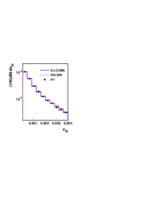
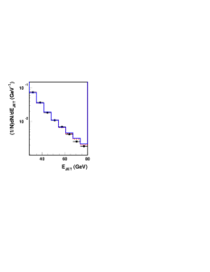
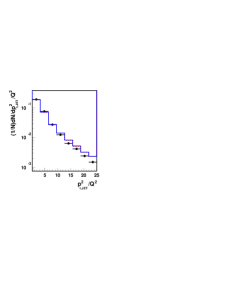
Forward jets with $0.5<p^{2}_{t,jet}/Q^{2}<5$

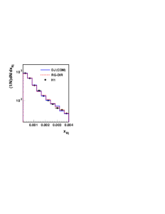
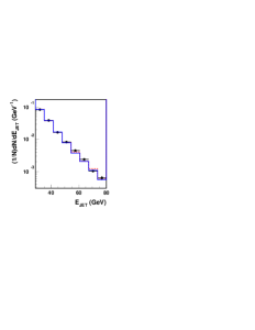
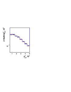
Figure 2: Control plots for the forward jet selection. The sample with no $p_{t,jet}^{2}/Q^{2}$-cut applied (upper) and the sample with the $0.5<p_{t,jet}^{2}/Q^{2}<5$-cut applied (lower) are shown. The distributions are at detector level and normalised to unity. All variables are measured in the laboratory frame. Comparisons are made to the predictions of the DJANGO (full line) and RAPGAP (dashed line) Monte Carlo programs.

The hadron level cross sections are extracted by applying correction factors to the data in order to take detector effects into account. The correction factors are calculated as the ratio of the CDM Monte Carlo prediction at the hadron and detector levels, in a bin-by-bin procedure. These factors correct the data from detector level to non-radiative hadron level, i.e. the data are also corrected for QED radiative effects. RAPGAP and CDM give similar values over the full kinematic range covered in this investigation. The correction factors are generally between 0.7 and 1.2 but in a few kinematic bins they reach values of 0.5 or 1.4 due to limited resolution of the jet quantities. The variations in the correction factors between the two Monte Carlo models are included in the systematic error.

The purity and acceptance are found to be larger than 30% in all bins. For the ‘2+forward jet’ analysis they are larger than 40% in all bins.

The systematic errors are estimated for each data point separately as the quadratic sum of the individual errors described below. The following systematic errors are considered:

• The hadronic energy scale uncertainty is determined to be 4%. In order to estimate the related uncertainty of the measured forward jet cross section, the reconstructed hadronic energies in the DJANGO/ARIADNE simulation were increased and decreased by this amount. The average resulting error is typically 8% for both the single differential forward jet cross section and the triple differential forward jet cross section, and 13% for the ‘2+forward jet’ cross section.

• The electromagnetic energy scale as measured in the SpaCal is known to an accuracy of 1%. Changing the scale by this amount in the forward jet cross section calculations using DJANGO/ARIADNE results in an average systematic error of typically 3% for the single and triple differential measurement, and 1% for the ‘2+forward jet’ measurement.

• The uncertainty on the measured scattering angle of the electron is estimated to be 1 mrad, which contributes typically 1% to the error in the forward and ‘2+forward jet’ cross section.

• The error from the model dependence is taken as the difference between the correction factors calculated from the DJANGO/ARIADNE and the RG-DIR Monte Carlo programs. Taking this variation into account yields a systematic error of about 5% for the single differential forward jet cross section, 8% for the triple differential case and 13% in the ‘2+forward jet’ cross section.

• The PHOJET [63, 64] Monte Carlo generator was used in order to estimate the extent to which DIS forward jet events could be faked by photoproduction ($Q^{2}\sim 0$ GeV²) background. The influence on the measurement is found to be negligible. The error attributed to this source of uncertainty is taken to be 1%.

• The uncertainty of the luminosity measurement is estimated to be 1.5%.

The averages of these sums are 10%, 12% and 14% for the single differential, triple differential and the ‘2+forward jet’ cross section, respectively. In the figures the systematic errors due to the energy scale uncertainty of the calorimeters ($\Delta_{\textrm{Syst1}}$) are shown separately as bands around the data points, whereas the other systematic errors ($\Delta_{\textrm{Syst2}}$) are included in the error bars together with the statistical errors. The errors are given separately in the tables.

6 Results

6.1 Single Differential Cross Section

The measurement of the single differential forward jet cross section is presented at the hadron level in the phase space region defined in section 4. The phase space for DGLAP evolution is suppressed by the additional requirement $0.5<p^{2}_{t,jet}/Q^{2}<5$ as discussed in section 4.

The measured single differential forward jet cross sections are listed in table 2. In Fig. 3a they are compared with LO ($\alpha_{s}$) and NLO ($\alpha^{2}_{s}$) calculations from DISENT. The calculations are multiplied by $(1+\delta_{\textrm{HAD}})$ to correct to the hadron level. The uncertainty from the factorisation and renormalisation scales, and the uncertainty in the PDF parametrisation, are added in quadrature to give the total theoretical error, which is shown as a band around the histogram presenting the theoretical prediction. In Fig. 3b and c the data are compared to the various QCD models.

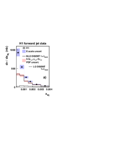
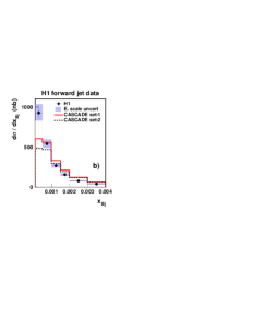
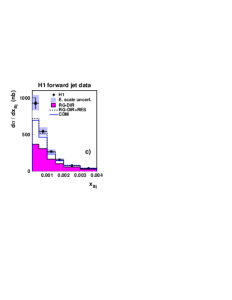
Figure 3: The hadron level cross section for forward jet production as a function of $x_{Bj}$ compared to NLO predictions from DISENT (a) and to QCD Monte Carlo models (b and c). The shaded band around the data points shows the error from the uncertainties in the calorimetric energy scales. The hatched band around the NLO calculations illustrates the theoretical uncertainties in the calculations, estimated as described in the text. The dashed line in (a) shows the LO contribution.

In Fig. 3a it can be observed that, at small $x_{Bj}$, the NLO di-jet calculations from DISENT are significantly larger than the LO contribution. This reflects the fact that the contribution from forward jets in the LO scenario is suppressed by kinematics. For small $x_{Bj}$ the NLO contribution is an order of magnitude larger than the LO contribution. The NLO contribution opens up the phase space for forward jets and improves the description of the data considerably. However, the NLO di-jet predictions are still a factor of 2 below the data at low $x_{Bj}$. The somewhat improved agreement at higher $x_{Bj}$ can be understood from the fact that the range in the longitudinal momentum fraction which is available for higher order emissions decreases.

From Fig. 3b it is seen that the CCFM model (both set-1 and set-2) predicts a somewhat harder $x_{Bj}$ distribution, which results in a comparatively poor description of the data.

Fig. 3c shows that the DGLAP model with direct photon interactions alone (RG-DIR) gives results similar to the NLO di-jet calculations and falls below the data, particularly in the low $x_{Bj}$ region. The description of the data by the DGLAP model is significantly improved if contributions from resolved virtual photon interactions are included (RG-DIR+RES). However, there is still a discrepancy in the lowest $x_{Bj}$-bin, where a possible BFKL signal would be expected to show up most prominently. The CDM model, which gives emissions that are non-ordered in transverse momentum, shows a behaviour similar to the RG DIR+RES model. Analytic calculations where resolved photon contributions are included to NLO order [53] again give similar agreement with the data as the RG DIR+RES model [22].

6.2 Triple Differential Cross Sections

In this section data are presented as triple differential forward jet cross sections. The total forward jet event sample is subdivided into bins of $Q^{2}$ and $p_{t,jet}^{2}$. The triple differential cross section $d\sigma/dx_{Bj}dQ^{2}dp_{t,jet}^{2}$ versus $x_{Bj}$ is shown in Figs. 4-6 for three regions in $Q^{2}$ and $p_{t,jet}^{2}$. Fig. 4 presents the cross section compared to NLO ($\alpha^{2}_{s}$) calculations, including theoretical errors, represented by error bands. In Fig. 5 and  6 comparisons to QCD Monte Carlo models are shown. The same parton density functions and scales are used as in the measurement of the single differential cross section. The cross section values are listed in table 3.

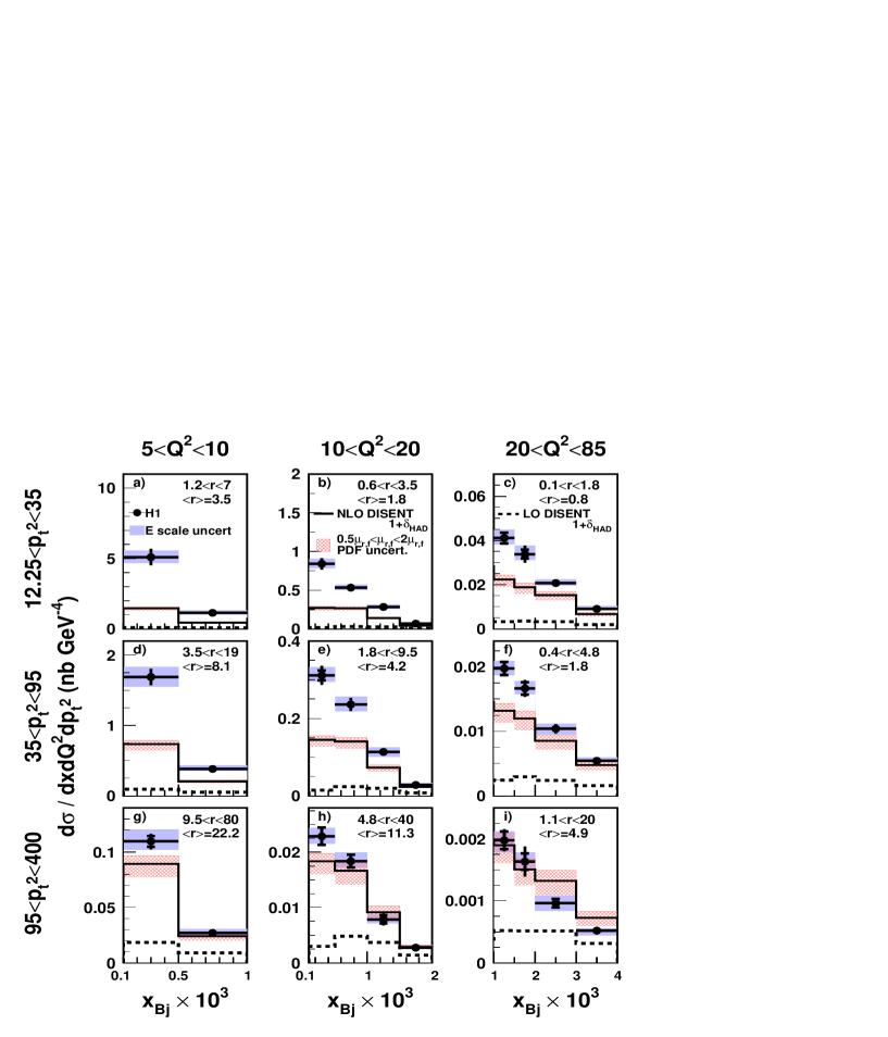
Figure 4: The hadron level triple differential cross section for forward jet production as a function of $x_{Bj}$, in bins of $Q^{2}$ (GeV²) and $p_{t,jet}^{2}$ (GeV²). The data are compared to the prediction of NLO (full line) and LO (dashed line) calculations from DISENT. Both calculations are corrected for hadronisation effects. The band around the data points illustrates the error due to the uncertainties in the calorimetric energy scales. The band around the NLO calculations illustrates the theoretical uncertainties in the calculations. In each bin the range in and the average value of $r=p_{t,jet}^{2}/Q^{2}$ is shown.

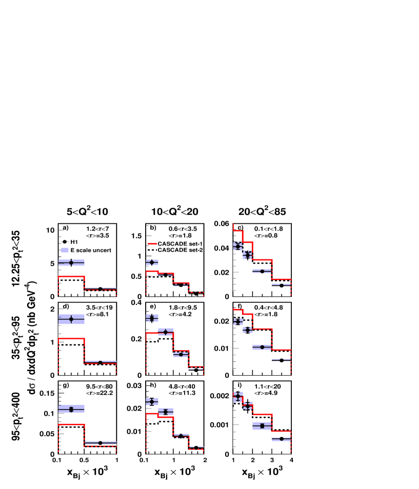
Figure 5: The hadron level triple differential cross section for forward jet production as a function of $x_{Bj}$, in bins of $Q^{2}$ (GeV²) and $p_{t,jet}^{2}$ (GeV²). The data are compared to the predictions of CASCADE. The band around the data points illustrates the error due to the uncertainties in the calorimetric energy scales. In each bin the range in and the average value of $r=p_{t,jet}^{2}/Q^{2}$ is shown.

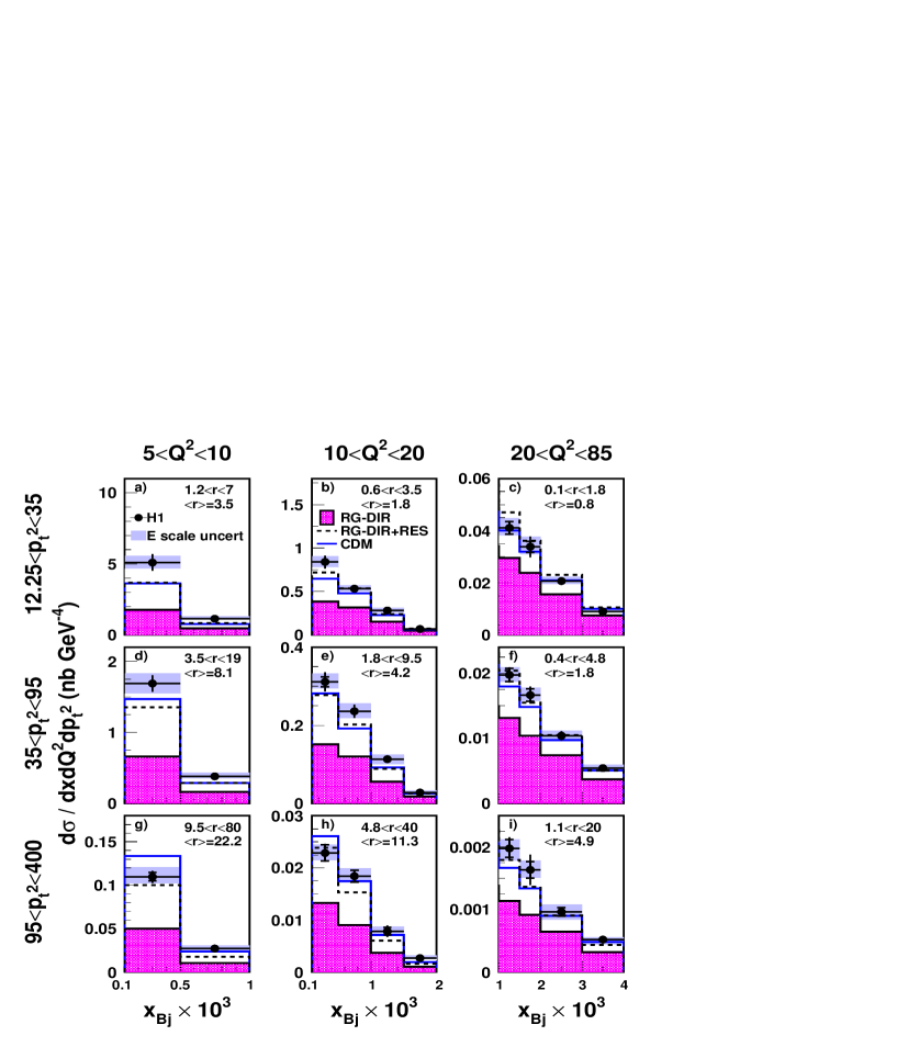
Figure 6: The hadron level triple differential cross section for forward jet production as a function of $x_{Bj}$, in bins of $Q^{2}$ (GeV²) and $p_{t,jet}^{2}$ (GeV²). The data are compared to the prediction of RAPGAP DIR, RAPGAP DIR+RES and CDM. The band around the data points illustrates the error due to the uncertainties in the calorimetric energy scales. In each bin the range in and the average value of $r=p_{t,jet}^{2}/Q^{2}$ is shown.

From Fig. 4 it can be observed that the NLO calculations in general undershoot the data but similarly to the single differential cross section the NLO calculations get closer to the data at higher $x_{Bj}$ and so too, due to the kinematics, at higher $Q^{2}$. The NLO calculations also give a better description of data for harder forward jets. In the highest $p_{t,jet}^{2}$-bin the difference between data and NLO is less than the (large) uncertainty in the NLO calculations in several $x_{Bj}$-bins. This is consistent with the results from a previous measurement on inclusive jet production [17]. A possible explanation is that jets with high $p_{t}$ remove a large fraction of the energy from the parton ladder, leaving limited energy available for additional emissions. Thus, the parton ladder is shorter and more like the NLO configuration. The general trend is that NLO calculations agree better with data as $x_{Bj}$, $Q^{2}$ and $p_{t,jet}^{2}$ increase. For high $p_{t,jet}$ the phase space for LO starts to open up, which also makes the NLO prediction more reliable.

The comparisons between data and QCD models are discussed in three different kinematic regions as specified below. These regions are however not strictly separated, but overlap. In all three regions the CDM and DGLAP resolved (RG-DIR+RES) models give very similar predictions (see Fig. 6) indicating that a breaking of the ordering of the virtuality is necessary to describe the data. As already observed in the single differential measurement the CCFM model predicts a somewhat harder $x_{Bj}$ distribution than seen in the data. This is true for the full kinematic range and leads to the poor description of the data as seen in Fig. 5.

$p_{t,jet}^{2}\sim Q^{2}$ $(r\sim 1)$

In this region events with parton emissions ordered in $p_{t}$ are suppressed, and thus parton dynamics beyond DGLAP may show up. The data are best described by the DGLAP resolved model (RG-DIR+RES) as observed in Fig. 6b and f.

$p_{t,jet}^{2}<Q^{2}$ $(r<1)$

The region where $Q^{2}$ might become larger than $p_{t,jet}^{2}$ is dominated by direct photon interactions. However, since $r$ can take values up to 1.8 in the most DGLAP-like bin (Fig. 6c), events with $p_{t,jet}^{2}$ of the same order or even greater than $Q^{2}$ are also contributing. This gives an admixture of events with emissions non-ordered in virtuality. This may explain why the DGLAP direct model (RG-DIR), although closer to the data in this region than in others, does not give good agreement with the data except for the highest $x_{Bj}$-bin. The CDM and DGLAP resolved model (RG-DIR+RES) reproduce the data very well in this region.

$p_{t,jet}^{2}>Q^{2}$ $(r>1)$

The kinematic region where $p_{t,jet}^{2}$ is larger than $Q^{2}$ is typical for processes where the virtual photon is resolved. As expected the DGLAP resolved model (RG-DIR+RES) provides a good overall description of the data, again similar to the CDM model. However, it can be noted that in the regions where $r$ is the highest and $x_{Bj}$ small, CDM shows a tendency to overshoot the data. DGLAP direct (RG-DIR) gives cross sections which are too low (see Fig. 6 d, g and h).

6.3 Events with Reconstructed Di-jets in Addition to the Forward Jet

Complementary to the analyses reported in sections 6.1 and 6.2, where the ratio $p_{t,jet}^{2}/Q^{2}$ has been used to isolate regions where a possible BFKL signal is enhanced, another method is used to control the evolution kinematics in the analysis reported here. By requiring the reconstruction of the two hardest jets in the event in addition to the forward jet, different kinematic regions can be investigated by applying cuts on the jet momenta and their rapidity separation as described in more detail in section 4.

In this scenario it is demanded that all jets have transverse momenta larger than 6 GeV. By applying the same $p_{t,jet}$-cut to all three jets, evolution with strong $k_{t}$-ordering is not favoured. Decreasing the $p_{t,jet}$-cut is not possible in this analysis due to detector resolutions. The jets are ordered in rapidity according to $\eta_{fwdjet}>\eta_{jet_{2}}>\eta_{jet_{1}}>\eta_{e}$ with $\eta_{e}$ being the rapidity of the scattered electron. The cross section is measured in two intervals of $\Delta\eta_{1}=\eta_{jet_{2}}-\eta_{jet_{1}}$. If the di-jet system originates from the quarks $q_{1}$ and $q_{2}$ (see Fig. 7), the phase space for evolution in $x$ between the di-jet system and the forward jet is increased by requiring that $\Delta\eta_{1}$ is small and that $\Delta\eta_{2}=\eta_{fwdjet}-\eta_{jet_{2}}$ is large. $\Delta\eta_{1}<1$ favours small invariant masses of the di-jet system and thereby small values of $x_{g}$ (see Fig. 7). With $\Delta\eta_{2}$ large, $x_{g}$ carries only a small fraction of the total propagating momentum, leaving the rest for additional radiation. It should be kept in mind, however, that only the forward jet is explicitely restricted in rapidity space, by the demand that it has to be close to the proton axis. The directions of the other jets are related to the forward jet through the $\Delta\eta$ requirements. When $\Delta\eta_{2}$ is small, it is therefore possible that one or both of the additional jets originate from gluon radiation close in rapidity space to the forward jet. With $\Delta\eta_{1}$ large, BFKL-like evolution may then occur between the two jets from the di-jet system, or, with both $\Delta\eta_{1}$ and $\Delta\eta_{2}$ small, even between the di-jet system and the hard scattering vertex. By studying the cross section for different $\Delta\eta$ values one can test theory and models for event topologies where the $k_{t}$ ordering is broken at varying locations along the evolution chain.

Figure 7: A schematic diagram of an event giving a forward jet and two additional hard jets. These may stem from the quarks ($q_{1}$ and $q_{2}$) in the hard scattering vertex or from gluons in the parton ladder. $x_{g}$ is the longitudinal momentum fraction carried by the gluon, connecting to the hard di-jet system (in this case $q_{1}$ and $q_{2}$) .

The cross sections for events containing a di-jet system in addition to the forward jet are presented as a function of $\Delta\eta_{2}$ in Figs. 8-10 for all ‘2+forward jet’ events , and for the requirements $\Delta\eta_{1}<1$ and $\Delta\eta_{1}>1$, respectively. The measured cross sections are given in table 4. For the $\Delta\eta_{1}<1$ region the cross section falls at low $\Delta\eta_{2}$ since the phase space becomes smaller when the 3 jets are forced to be close together. Fig. 8 gives a comparison of data to NLO ($\alpha^{3}_{s}$) predictions with theoretical error contributions included as bands. In Figs. 9 and 10 comparisons to QCD models are presented.

In this investigation the same settings of the QCD models are used as in sections 6.1 and  6.2, while the NLO three-jet cross sections are calculated using NLOJET++.

From Fig. 8 it is observed that NLOJET++ gives good agreement with the data if the two additional hard jets are emitted in the central region ($\Delta\eta_{2}$ large). It is interesting to note that a fixed order calculation ($\alpha_{s}^{3}$), including the $\log(1/x)$-term to the first order in $\alpha_{s}$, is able to describe these data well. However, the more the additional hard jets are shifted to the forward region ($\Delta\eta_{2}$ small), the less well are the data described by NLOJET++. This can be understood from the fact that the more forward the additional jets go, the higher the probability is that one of them, or even both, do not actually originate from quarks but from additional radiated gluons. For gluon induced processes, which dominate at small $x$, NLOJET++ calculates the NLO contribution to final states containing one gluon jet and two jets from the di-quarks, i.e. it accounts for the emission of one gluon in addition to the three jets. Thus, events where two of the three selected jets originate from gluons are produced by NLOJET++ only in the real emission corrections to the three-jet final state, which effectively means that these kinematic configurations are only produced to leading order ($\alpha_{s}^{3}$). The most extreme case, where all three reconstructed jets are produced by gluons, is not considered by NLOJET++. This results in a depletion of the theoretical cross section in the small $\Delta\eta_{2}$ region, which is more pronounced when $\Delta\eta_{1}$ is also small, i.e. when all three jets are in the forward region. Consequently a significant deviation between data and NLOJET++ can be observed for such events (see the lowest bin in Fig. 8b). Accounting for still higher orders in $\alpha_{s}$ might improve the description of the data in this domain since virtual corrections to the production of two gluons could increase the cross section for such final states, and additional gluon emissions would enhance the probability that one of the soft radiated gluons produces a jet that fulfills the transverse momentum requirement applied in this analysis.

For the ‘2+forward jet’ sample CCFM is not describing well the shape of the $\eta$-distributions (Fig. 9a, b and c).

As explained above, evolution with strong $k_{t}$-ordering is disfavoured in this study. Radiation that is non-ordered in $k_{t}$ may occur at different locations along the evolution chain, depending on the values of $\Delta\eta_{1}$ and $\Delta\eta_{2}$. As can be seen from Fig. 10, the colour dipole model gives good agreement in all cases, whereas the DGLAP models give cross sections that are too low except when both $\Delta\eta_{1}$ and $\Delta\eta_{2}$ are large. For this last topology all models and the NLO calculation agree with the data, indicating that the available phase space is exhausted and that little freedom is left for dynamical variations.

If one or both jets from the di-jet system are produced by gluon radiation, which is increasingly probable the more forward these jets go, it necessarily means that the $k_{t}$ ordering is broken. In this context it is noteworthy that CDM provides the best description of the data while the other models, including the DGLAP-resolved model, fail in most of the bins. The ‘2+forward jet’ sample differentiates CDM and the DGLAP-resolved model, in contrast to the more inclusive samples where CDM and RG-DIR+RES give the same predictions. The conclusion is that additional breaking of the $k_{t}$ ordering is needed compared to what is included in the resolved photon model.

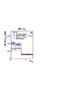
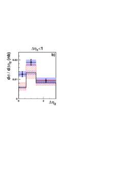
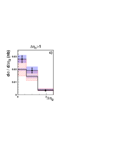
Figure 8: The cross section for events with a reconstructed high transverse momentum di-jet system and a forward jet as a function of the rapidity separation between the forward jet and the most forward-going additional jet, $\Delta\eta_{2}$. Results are shown for the full sample and for two ranges of the separation between the two additional jets, $\Delta\eta_{1}<1$ and $\Delta\eta_{1}>1$. The data are compared to the predictions of a three-jet NLO calculations from NLOJET++ $(1+\delta_{\textrm{HAD}})$. The band around the data points illustrates the error due to the uncertainties in the calorimetric energy scales. The band around the NLO calculations illustrates the theoretical uncertainties in the calculations.

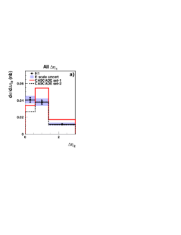
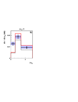
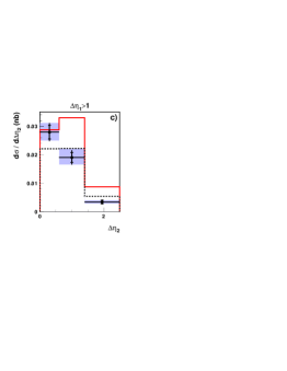
Figure 9: The cross section for events with a reconstructed high transverse momentum di-jet system and a forward jet as a function of the rapidity separation between the forward jet and the most forward-going additional jet, $\Delta\eta_{2}$. Results are shown for the full sample and for two ranges of the separation between the two additional jets, $\Delta\eta_{1}<1$ and $\Delta\eta_{1}>1$. The data are compared to the predictions of CASCADE. The band around the data points illustrates the error due to the uncertainties in the calorimetric energy scales.

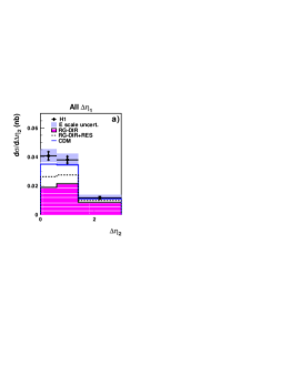
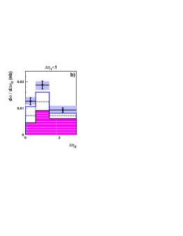
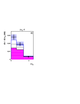
Figure 10: The cross section for events with a reconstructed high transverse momentum di-jet system and a forward jet as a function of the rapidity separation between the forward jet and the most forward-going additional jet, $\Delta\eta_{2}$. Results are shown for the full sample and for two ranges of the separation between the two additional jets, $\Delta\eta_{1}<1$ and $\Delta\eta_{1}>1$. The data are compared to the predictions of RAPGAP DIR, RAPGAP DIR+RES and CDM. The band around the data points illustrates the error due to the uncertainties in the calorimetric energy scales.

7 Summary

An investigation of DIS events containing a jet in the forward direction is presented. Various constraints are applied, which suppress contributions to the parton evolution described by the DGLAP equations and enhance the sensitivity to other parton dynamics. Several observables involving forward jet events are studied and compared to the predictions of NLO calculations and QCD models.

Leading order ($\alpha_{s}$) calculations of the single differential forward jet cross section, $d\sigma/dx_{Bj}$, are well below the measurements, which is expected since forward jet production is kinematically suppressed in LO. NLO di-jet calculations improve the description of the data but remain too low at small values of $x_{Bj}$. This is also the case for predictions based on the DGLAP direct model. The DGLAP resolved photon model (RG-DIR+RES) and the colour dipole model (CDM) come closest to the data.

The total forward jet sample is subdivided into bins of $Q^{2}$ and $p_{t,jet}^{2}$ such that kinematic regions are defined in which the effects of different evolution dynamics are enhanced. In the most DGLAP enhanced region, ($Q^{2}\gg p_{t,jet}^{2}$), and in the region where contributions from resolved processes are expected to become important ($p_{t,jet}^{2}\gg Q^{2}$), the measured triple differential forward jet cross sections are well described by the CDM and the DGLAP resolved model (RG-DIR+RES). In the BFKL region ($Q^{2}\sim p_{t,jet}^{2}$) the CDM and DGLAP resolved model (RG-DIR+RES) again reproduce the data best. A general observeration is that the DGLAP resolved model and CDM tend to fall below the data at low $x_{Bj}$, $Q^{2}$ and $p^{2}_{t}$. The cross sections predicted by the DGLAP direct model (RG-DIR) are consistently too low in all regions and especially at low $x_{Bj}$.

The NLO di-jet calculations from DISENT describe the data for the largest values of $x_{Bj}$ at high values of $Q^{2}$ and $p^{2}_{t}$, but fail for low values of these variables.

The measured cross section for events with a reconstructed di-jet system in addition to the forward jet are in good agreement with the predictions of NLOJET++  if the additional jets are emitted in the central region. As expected, deviations are observed for other jet topologies. The data are best described by the CDM. The DGLAP resolved model (RG-DIR+RES) is below the data as is, to an even greater extent, the DGLAP direct model (RG-DIR). This result gives the first evidence for parton dynamics in which there is additional breaking of the $k_{t}$-ordering compared to that provided by the resolved photon model.

The CCFM model, as implemented in CASCADE, with two different parametrisations of the unintegrated gluon density, fails to describe the shape of both the single and triple differential cross sections, as well as the ‘2+forward jet’ cross section. This might be caused by the parametrisation of the unintegrated gluon density and/or the missing contributions from splittings into quark pairs.

The observations made here demonstrate that an accurate description of the radiation pattern at small $x_{Bj}$ requires the introduction of terms beyond those included in the DGLAP direct approximation (RG-DIR). Higher order parton emissions with breaking of the transverse momentum ordering contribute noticeably to the cross section. Calculations which include such processes, such as CDM and the resolved photon model, provide a better description of the data. The similar behaviour of CDM and the DGLAP resolved model (RG-DIR+RES), which describe the data best, indicates that the inclusive forward jet measurements do not give a significant separation of the models. However, in the more exclusive measurement of ‘2+forward jet’ events a clear differentiation of the models is obtained since, in contrast to CDM, the DGLAP resolved model (RG-DIR+RES) fails to describe the data.

$x_{Bj}$	$d\sigma/dx_{Bj}$ (nb)	$\Delta_{\textrm{Stat}}$ (nb)	$\Delta_{\textrm{Syst1}}$ (nb)	$\Delta_{\textrm{Syst2}}$ (nb)
0.0001-0.0005	925	$\pm$ 17	$+110\atop-100$	$+77\atop-77$
0.0005-0.001	541	$\pm$ 12	$+54\atop-55$	$+23\atop-24$
0.001-0.0015	264	$\pm$ 8	$+30\atop-28$	$+11\atop-11$
0.0015-0.002	153	$\pm$ 6	$+19\atop-16$	$+8\atop-8$
0.002-0.003	74.5	$\pm$ 3.0	$+10.7\atop-8.0$	$+1.9\atop-1.8$
0.003-0.004	36.7	$\pm$ 2.0	$+2.1\atop-5.7$	$+2.4\atop-2.4$

Table 2: Single differential forward jet cross sections in bins of $x_{Bj}$. The statistical error ($\Delta_{\textrm{Stat}}$), the error from the uncertainty of the calorimetric energy scales ($\Delta_{\textrm{Syst1}}$) and from the other systematic errors ($\Delta_{\textrm{Syst2}}$) are specified.

$Q^{2}\atop(\textrm{GeV}^{2})$	$p^{2}_{t}\atop(\textrm{GeV}^{2})$	$x_{Bj}$	$d^{3}\sigma/dx_{Bj}dQ^{2}dp^{2}_{t}\atop(\textrm{nb GeV}^{-4})$	$\Delta_{\textrm{Stat}}\atop(\textrm{nb})$	$\Delta_{\textrm{Syst1}}\atop(\textrm{nb})$	$\Delta_{\textrm{Syst2}}\atop(\textrm{nb})$
	12.25-35	0.0001-0.0005	5.10	$\pm$ 0.12	$+0.46\atop-0.44$	$+0.58\atop-0.59$
		0.0005-0.001	1.13	$\pm$ 0.05	$+0.16\atop-0.07$	$+0.17\atop-0.17$
5-10	35-95	0.0001-0.0005	1.70	$\pm$ 0.04	$+0.14\atop-0.14$	$+0.11\atop-0.11$
		0.0005-0.001	3.81$\cdot 10^{-1}$	$\pm$ 0.18$\cdot 10^{-1}$	$+0.51\cdot 10^{-1}\atop-0.33\cdot 10^{-1}$	$+0.13\cdot 10^{-1}\atop-0.10\cdot 10^{-1}$
	95-400	0.0001-0.0005	1.11$\cdot 10^{-1}$	$\pm$ 0.05$\cdot 10^{-1}$	$+0.11\cdot 10^{-1}\atop-0.08\cdot 10^{-1}$	$+0.05\cdot 10^{-1}\atop-0.05\cdot 10^{-1}$
		0.0005-0.001	2.71$\cdot 10^{-2}$	$\pm$ 0.22$\cdot 10^{-2}$	$+0.35\cdot 10^{-2}\atop-0.33\cdot 10^{-2}$	$+0.26\cdot 10^{-2}\atop-0.26\cdot 10^{-2}$
	12.25-35	0.0001-0.0005	8.40$\cdot 10^{-1}$	$\pm$ 0.31$\cdot 10^{-1}$	$+0.64\cdot 10^{-1}\atop-0.62\cdot 10^{-1}$	$+0.67\cdot 10^{-1}\atop-0.66\cdot 10^{-1}$
		0.0005-0.001	5.31$\cdot 10^{-1}$	$\pm$ 0.24$\cdot 10^{-1}$	$+0.39\cdot 10^{-1}\atop-0.34\cdot 10^{-1}$	$+0.22\cdot 10^{-1}\atop-0.22\cdot 10^{-1}$
		0.001-0.0015	2.81$\cdot 10^{-1}$	$\pm$ 0.16$\cdot 10^{-1}$	$+0.32\cdot 10^{-1}\atop-0.29\cdot 10^{-1}$	$+0.36\cdot 10^{-1}\atop-0.37\cdot 10^{-1}$
		0.0015-0.002	6.67$\cdot 10^{-2}$	$\pm$ 0.73$\cdot 10^{-2}$	$+0.38\cdot 10^{-2}\atop-0.65\cdot 10^{-2}$	$+0.09\cdot 10^{-2}\atop-0.08\cdot 10^{-2}$
	35-95	0.0001-0.0005	3.11$\cdot 10^{-1}$	$\pm$ 0.13$\cdot 10^{-1}$	$+0.21\cdot 10^{-1}\atop-0.17\cdot 10^{-1}$	$+0.21\cdot 10^{-1}\atop-0.21\cdot 10^{-1}$
10-20		0.0005-0.001	2.36$\cdot 10^{-1}$	$\pm$ 0.09$\cdot 10^{-1}$	$+0.20\cdot 10^{-1}\atop-0.18\cdot 10^{-1}$	$+0.14\cdot 10^{-1}\atop-0.15\cdot 10^{-1}$
		0.001-0.0015	1.13$\cdot 10^{-1}$	$\pm$ 0.06$\cdot 10^{-1}$	$+0.12\cdot 10^{-1}\atop-0.13\cdot 10^{-1}$	$+0.03\cdot 10^{-1}\atop-0.03\cdot 10^{-1}$
		0.0015-0.002	2.81$\cdot 10^{-2}$	$\pm$ 0.33$\cdot 10^{-2}$	$+0.50\cdot 10^{-2}\atop-0.19\cdot 10^{-2}$	$+0.27\cdot 10^{-2}\atop-0.22\cdot 10^{-2}$
	95-400	0.0001-0.0005	2.29$\cdot 10^{-2}$	$\pm$ 0.16$\cdot 10^{-2}$	$+0.15\cdot 10^{-2}\atop-0.15\cdot 10^{-2}$	$+0.08\cdot 10^{-2}\atop-0.07\cdot 10^{-2}$
		0.0005-0.001	1.84$\cdot 10^{-2}$	$\pm$ 0.11$\cdot 10^{-2}$	$+0.16\cdot 10^{-2}\atop-0.13\cdot 10^{-2}$	$+0.04\cdot 10^{-2}\atop-0.05\cdot 10^{-2}$
		0.001-0.0015	7.83$\cdot 10^{-3}$	$\pm$ 0.74$\cdot 10^{-3}$	$+0.87\cdot 10^{-3}\atop-0.75\cdot 10^{-3}$	$+0.83\cdot 10^{-3}\atop-0.79\cdot 10^{-3}$
		0.0015-0.002	2.70$\cdot 10^{-3}$	$\pm$ 0.45$\cdot 10^{-3}$	$+0.46\cdot 10^{-3}\atop-0.27\cdot 10^{-3}$	$+0.35\cdot 10^{-3}\atop-0.39\cdot 10^{-3}$
	12.25-35	0.001-0.0015	4.11$\cdot 10^{-2}$	$\pm$ 0.24$\cdot 10^{-2}$	$+0.37\cdot 10^{-2}\atop-0.30\cdot 10^{-2}$	$+0.12\cdot 10^{-2}\atop-0.12\cdot 10^{-2}$
		0.0015-0.002	3.38$\cdot 10^{-2}$	$\pm$ 0.21$\cdot 10^{-2}$	$+0.38\cdot 10^{-2}\atop-0.29\cdot 10^{-2}$	$+0.34\cdot 10^{-2}\atop-0.34\cdot 10^{-2}$
		0.002-0.003	2.07$\cdot 10^{-2}$	$\pm$ 0.12$\cdot 10^{-2}$	$+0.16\cdot 10^{-2}\atop-0.13\cdot 10^{-2}$	$+0.06\cdot 10^{-2}\atop-0.07\cdot 10^{-2}$
		0.003-0.004	9.03$\cdot 10^{-3}$	$\pm$ 0.79$\cdot 10^{-3}$	$+1.37\cdot 10^{-3}\atop-0.12\cdot 10^{-3}$	$+0.44\cdot 10^{-3}\atop-0.44\cdot 10^{-3}$
	35-95	0.001-0.0015	1.97$\cdot 10^{-2}$	$\pm$ 0.10$\cdot 10^{-2}$	$+0.11\cdot 10^{-2}\atop-0.11\cdot 10^{-2}$	$+0.06\cdot 10^{-2}\atop-0.05\cdot 10^{-2}$
20-85		0.0015-0.002	1.67$\cdot 10^{-2}$	$\pm$ 0.10$\cdot 10^{-2}$	$+0.11\cdot 10^{-2}\atop-0.10\cdot 10^{-2}$	$+0.09\cdot 10^{-2}\atop-0.09\cdot 10^{-2}$
		0.002-0.003	1.04$\cdot 10^{-2}$	$\pm$ 0.06$\cdot 10^{-2}$	$+0.08\cdot 10^{-2}\atop-0.10\cdot 10^{-2}$	$+0.05\cdot 10^{-2}\atop-0.05\cdot 10^{-2}$
		0.003-0.004	5.45$\cdot 10^{-3}$	$\pm$ 0.39$\cdot 10^{-3}$	$+0.46\cdot 10^{-3}\atop-0.24\cdot 10^{-3}$	$+0.46\cdot 10^{-3}\atop-0.46\cdot 10^{-3}$
	95-400	0.001-0.0015	1.98$\cdot 10^{-3}$	$\pm$ 0.14$\cdot 10^{-3}$	$+0.15\cdot 10^{-3}\atop-0.20\cdot 10^{-3}$	$+0.11\cdot 10^{-3}\atop-0.11\cdot 10^{-3}$
		0.0015-0.002	1.63$\cdot 10^{-3}$	$\pm$ 0.13$\cdot 10^{-3}$	$+0.15\cdot 10^{-3}\atop-0.13\cdot 10^{-3}$	$+0.20\cdot 10^{-3}\atop-0.20\cdot 10^{-3}$
		0.002-0.003	9.64$\cdot 10^{-4}$	$\pm$ 0.70$\cdot 10^{-4}$	$+1.15\cdot 10^{-4}\atop-1.35\cdot 10^{-4}$	$+0.07\cdot 10^{-4}\atop-0.07\cdot 10^{-4}$
		0.003-0.004	5.17$\cdot 10^{-4}$	$\pm$ 0.49$\cdot 10^{-4}$	$+0.41\cdot 10^{-4}\atop-0.81\cdot 10^{-4}$	$+0.06\cdot 10^{-4}\atop-0.03\cdot 10^{-4}$

Table 3: Triple differential cross sections in bins of $Q^{2}$, $p^{2}_{t}$ and $x_{Bj}$. The statistical error ($\Delta_{\textrm{Stat}}$), the error from the uncertainty of the calorimetric energy scales ($\Delta_{\textrm{Syst1}}$) and from the other systematic errors ($\Delta_{\textrm{Syst2}}$) are specified.

$\Delta\eta_{1}$	$\Delta\eta_{2}$	$d\sigma/d\Delta\eta_{2}$ (pb)	$\Delta_{\textrm{Stat}}$ (pb)	$\Delta_{\textrm{Syst1}}$ (pb)	$\Delta_{\textrm{Syst2}}$ (nb)
	0.0 - 0.6	40.6	$\pm 2.7$	$+4.8\atop-4.4$	$+2.1\atop-2.2$
All $\Delta\eta_{1}$	0.6 - 1.4	37.9	$\pm 2.2$	$+4.3\atop-4.4$	$+2.2\atop-2.2$
	1.4 - 3.0	11.6	$\pm 1.0$	$+2.0\atop-1.5$	$+0.2\atop-0.2$
	0.0 - 0.6	12.7	$\pm 1.3$	$+1.5\atop-1.3$	$+0.3\atop-0.4$
$\Delta\eta_{1}<1$	0.6 - 1.4	18.8	$\pm 1.5$	$+1.4\atop-1.9$	$+0.4\atop-0.4$
	1.4 - 3.0	9.3	$\pm 0.9$	$+1.6\atop-1.0$	$+0.3\atop-0.3$
	0.0 - 0.6	27.9	$\pm 2.4$	$+3.2\atop-3.0$	$+2.1\atop-2.1$
$\Delta\eta_{1}>1$	0.6 - 1.4	19.0	$\pm 1.7$	$+3.0\atop-2.6$	$+1.8\atop-1.9$
	1.4 - 2.5	3.4	$\pm 0.6$	$+0.5\atop-0.6$	$+0.5\atop-0.5$

Table 4: ‘2+forward jet’ cross sections in bins of $\Delta\eta_{2}$ for all $\Delta\eta_{1}$, $\Delta\eta_{1}<1$ and $\Delta\eta_{1}>1$. The statistical error ($\Delta_{\textrm{Stat}}$), the error from the uncertainty of the calorimetric energy scales ($\Delta_{\textrm{Syst1}}$) and from the other systematic errors ($\Delta_{\textrm{Syst2}}$) are specified.

8 Acknowledgement

We are grateful to the HERA machine group whose outstanding efforts have made and continue to make this experiment possible. We thank the engineers and technicians for their work in constructing and maintaining the H1 detector, our funding agencies for financial support, the DESY technical staff for continual assistance and the DESY directorate for hospitality which they extend to the non-DESY members of the collaboration. J. Bartels, G. Gustafson and L. Lönnblad are acknowledged for valuable discussions concerning the interpretation of the results.

References

- [1] V. N. Gribov and L. N. Lipatov, Sov. J. Nucl. Phys. 15 (1972) 675 [Yad. Fiz. 15 (1972) 1218].
- [2] V. N. Gribov and L. N. Lipatov, Sov. J. Nucl. Phys. 15 (1972) 438 [Yad. Fiz. 15 (1972) 781].
- [3] L. N. Lipatov, Sov. J. Nucl. Phys. 20 (1975) 94 [Yad. Fiz. 20 (1974) 181].
- [4] G. Altarelli and G. Parisi, Nucl. Phys. B 126 (1977) 298.
- [5] Y. L. Dokshitzer, Sov. Phys. JETP 46 (1977) 641 [Zh. Eksp. Teor. Fiz. 73 (1977) 1216].
- [6] C. Adloff et al. [H1 Collaboration], Eur. Phys. J. C 13 (2000) 609 [hep-ex/9908059].
- [7] C. Adloff et al. [H1 Collaboration], Eur. Phys. J. C 21 (2001) 33 [hep-ex/0012053].
- [8] S. Chekanov et al. [ZEUS Collaboration], Eur. Phys. J. C 21 (2001) 443 [hep-ex/0105090].
- [9] S. Chekanov et al. [ZEUS Collaboration], Phys. Rev. D 70 (2004) 052001 [hep-ex/0401003].
- [10] E. A. Kuraev, L. N. Lipatov and V. S. Fadin, Sov. Phys. JETP 44 (1976) 443 [Zh. Eksp. Teor. Fiz. 71 (1976) 840].
- [11] E. A. Kuraev, L. N. Lipatov and V. S. Fadin, Sov. Phys. JETP 45 (1977) 199 [Zh. Eksp. Teor. Fiz. 72 (1977) 377].
- [12] I. I. Balitsky and L. N. Lipatov, Sov. J. Nucl. Phys. 28 (1978) 822 [Yad. Fiz. 28 (1978) 1597].
- [13] C. Adloff et al. [H1 Collaboration], Eur. Phys. J. C 13 (2000) 397 [hep-ex/9812024].
- [14] C. Adloff et al. [H1 Collaboration], Eur. Phys. J. C 13 (2000) 415 [hep-ex/9806029].
- [15] S. Chekanov et al. [ZEUS Collaboration], Eur. Phys. J. C 23 (2002) 13 [hep-ex/0109029].
- [16] C. Adloff et al. [H1 Collaboration], Phys. Lett. B 415 (1997) 418 [hep-ex/9709017].
- [17] C. Adloff et al. [H1 Collaboration], Phys. Lett. B 542 (2002) 193 [hep-ex/0206029].
- [18] S. Aid et al. [H1 Collaboration], Phys. Lett. B 356 (1995) 118 [hep-ex/9506012].
- [19] C. Adloff et al. [H1 Collaboration], Eur. Phys. J. C 12 (2000) 595 [hep-ex/9907027].
- [20] C. Adloff et al. [H1 Collaboration], Nucl. Phys. B 485 (1997) 3 [hep-ex/9610006].
- [21] J. Breitweg et al. [ZEUS Collaboration], Phys. Lett. B 479 (2000) 37 [hep-ex/0002010].
- [22] H. Jung, L. Jönsson and H. Küster, “Resolved photon processes in DIS and small x dynamics,” [hep-ph/9805396].
- [23] H. Jung, L. Jönsson and H. Küster, Eur. Phys. J. C 9 (1999) 383 [hep-ph/9903306].
- [24] A. Aktas et al. [H1 Collaboration], Eur. Phys. J. C 37 (2004) 141 [hep-ex/0401010].
- [25] C. Adloff et al. [H1 Collaboration], Phys. Lett. B 462 (1999) 440 [hep-ex/9907030].
- [26] A. Aktas et al. [H1 Collaboration], Eur. Phys. J. C 36 (2004) 441 [hep-ex/0404009].
- [27] B. Andersson, G. Gustafson, L. Lönnblad and U. Pettersson, Z. Phys. C 43 (1989) 625.
- [28] L. Lönnblad, Z. Phys. C 65 (1995) 285.
- [29] C. Adloff et al. [H1 Collaboration], Nucl. Phys. B 538 (1999) 3 [hep-ex/9809028].
- [30] J. Breitweg et al. [ZEUS Collaboration], Eur. Phys. J. C 6 (1999) 239 [hep-ex/9805016].
- [31] S. Chekanov et al. [ZEUS Collaboration], hep-ex/0502029.
- [32] M. Ciafaloni, Nucl. Phys. B 296 (1988) 49.
- [33] S. Catani, F. Fiorani and G. Marchesini, Phys. Lett. B 234 (1990) 339.
- [34] S. Catani, F. Fiorani and G. Marchesini, Nucl. Phys. B 336 (1990) 18.
- [35] G. Marchesini, Nucl. Phys. B 445 (1995) 49 [hep-ph/9412327].
- [36] H. Jung, Comput. Phys. Commun. 86 (1995) 147.
- [37] A. Kwiatkowski, H. Spiesberger and H. J. Möhring, Comput. Phys. Commun. 69 (1992) 155.
- [38] K. Charchula, G. A. Schuler and H. Spiesberger, Comput. Phys. Commun. 81 (1994) 381.
- [39] L. Lönnblad, Comput. Phys. Commun. 71 (1992) 15.
- [40] J. Pumplin et al. JHEP 0207 (2002) 012 [hep-ph/0201195].
- [41] C. Adloff et al. [H1 Collaboration], Eur. Phys. J. C 19 (2001) 289 [hep-ex/0010054].
- [42] H. Jung and G. P. Salam, Eur. Phys. J. C 19 (2001) 351 [hep-ph/0012143].
- [43] H. Jung, Comput. Phys. Commun. 143 (2002) 100 [hep-ph/0109102].
- [44] M. Hansson and H. Jung, “Status of CCFM: Un-integrated gluon densities”, [hep-ph/0309009].
- [45] R. Brun, R. Hagelberg, M. Hansroul and J. C. Lassalle, CERN-DD-78-2-REV
- [46] S. Catani and M. H. Seymour, Phys. Lett. B 378 (1996) 287 [hep-ph/9602277].
- [47] S. Catani and M. H. Seymour, Nucl. Phys. B 485 (1997) 291 [Erratum-ibid. B 510 (1997) 503] [hep-ph/9605323].
- [48] M. A. Kimber, A. D. Martin and M. G. Ryskin, Phys. Rev. D 63 (2001) 114027 [hep-ph/0101348].
- [49] Z. Nagy and Z. Trocsanyi, Phys. Rev. Lett. 87 (2001) 082001 [hep-ph/0104315].
- [50] H. Jung, “Un-integrated PDFs in CCFM”, hep-ph/0411287.
- [51] H. Jung, Proceedings of the 12th International Workshop on Deep Inelastic Scattering (DIS 2004), Strbske Pleso, Slovakia, April 14-18, 2004, Eds. D. Bruncko, J. Ferencei and P. Strizenec, Inst. Exp. Phys. SAS, 2004, Kosice, Vol 1, p.299.
- [52] G. A. Schuler and T. Sjöstrand, Phys. Lett. B 376 (1996) 193 [hep-ph/9601282].
- [53] G. Kramer and B. Pötter, Phys. Lett. B 453 (1999) 295 [hep-ph/9901314].
- [54] I. Abt et al. [H1 Collaboration], Nucl. Instrum. Meth. A 386 (1997) 348.
- [55] I. Abt et al. [H1 Collaboration], Nucl. Instrum. Meth. A 386 (1997) 310.
- [56] R. D. Appuhn et al. [H1 SPACAL Group], Nucl. Instrum. Meth. A 386 (1997) 397.
- [57] B. Andrieu et al. [H1 Calorimeter Group Collaboration], Nucl. Instrum. Meth. A 336 (1993) 499.
- [58] A. H. Mueller, Nucl. Phys. Proc. Suppl. 18C, 125 (1991).
- [59] A. H. Mueller, J. Phys. G 17 (1991) 1443.
- [60] S. Catani, Y. L. Dokshitzer, M. H. Seymour and B. R. Webber, Nucl. Phys. B 406 (1993) 187.
- [61] S. Catani, Y. L. Dokshitzer and B. R. Webber, Phys. Lett. B 285 (1992) 291.
- [62] C. Adloff et al. [H1 Collaboration], Z. Phys. C 74 (1997) 221 [hep-ex/9702003].
- [63] R. Engel and J. Ranft, Phys. Rev. D 54 (1996) 4244 [hep-ph/9509373].
- [64] R. Engel, Z. Phys. C 66 (1995) 203.