Model Independent Measurement of $S\hbox{-wave}$ $K^{-}\pi^{+}$ systems using $D^{+}\rightarrow K\pi\pi$ Decays from Fermilab E791.

Abstract

A model-independent partial-wave analysis of the $S\hbox{-wave}$ component of the $K\pi$ system from decays of $D^{+}$ mesons to the three-body $K^{-}\pi^{+}\pi^{+}$ final state is described. Data come from the Fermilab E791 experiment. Amplitude measurements are made independently for ranges of $K^{-}\pi^{+}$ invariant mass, and results are obtained below 825 $\hbox{MeV}/c^{2}$, where previous measurements exist only in two mass bins. This method of parametrizing a three-body decay amplitude represents a new approach to analysing such decays. Though no model is required for the $S\hbox{-wave}$, a parametrization of the relatively well-known reference $P\hbox{-}$ and $D\hbox{-wave}$s, optimized to describe the data used, is required. In this paper, a Breit-Wigner model is adopted to describe the resonances in these waves. The observed phase variation for the $S\hbox{-}$, $P\hbox{-}$ and $D\hbox{-wave}$s do not match existing measurements of $I={1\over 2}$ $K^{-}\pi^{+}$ scattering in the invariant mass range in which scattering is predominantly elastic. If the data are mostly $I={1\over 2}$, this observation indicates that the Watson theorem, which requires these phases to have the same dependence on invariant mass, may not apply to these decays without allowing for some interaction with the other pion. The production rate of $K^{-}\pi^{+}$ from these decays, if assumed to be predominantly $I={1\over 2}$, is also found to have a significant dependence on invariant mass in the region above 1.25 $\hbox{GeV}/c^{2}$. These measurements can provide a relatively model-free basis for future attempts to determine which strange scalar amplitudes contribute to the decays.

I Introduction

Kinematics and angular momentum conservation in decays of ground state, heavy-quark mesons to three pseudoscalars strongly favor production of $S\hbox{-wave}$ systems. These decays have therefore been regarded as a source of information on the composition of the scalar meson (spin-parity $J^{P}=0^{+}$) spectrum. Extracting this information has, however, been done in model-dependent ways that can influence the outcome. For the di-meson subsystems, vector and tensor resonances are relatively well-understood, but, as larger samples of $D$ and $B$ meson decays become available, the correct modelling of the $S\hbox{-wave}$ contributions becomes an increasingly important factor in the task of obtaining satisfactory fits to the data.

Analyses typically use an isobar model formulation in which the decays are described by a coherent sum of a non-resonant three-body amplitude $NR$, usually taken to be constant in magnitude and phase over the entire Dalitz plot, and a number of quasi two-body (resonance + bachelor) amplitudes where the bachelor particle is one of the three final state products, and the resonance decays to the remaining pair. It is assumed that all resonant and $NR$ processes taking part in the decay are described by amplitudes that interfere, and have relative phases and magnitudes determined by the decay of the parent meson. In cases where all three decay products are pseudoscalar ($P$) particles, angular momentum conservation requires that the resonances produced are scalar ($S\hbox{-wave}$), vector ($P\hbox{-wave}$), etc . For $D$ mesons, decays beyond $D\hbox{-wave}$ are highly suppressed by the angular momentum barrier factor and can be neglected.

Within this formalism, the decays $D^{+}\rightarrow\pi^{-}\pi^{+}\pi^{+}$ and $D^{+}\rightarrow K^{-}\pi^{+}\pi^{+}$ con were once thought to require very large, constant $NR$ amplitudes Frabetti et al. (1994); Anjos et al. (1993); Frabetti et al. (1997). Using larger samples, the Fermilab E791 collaboration found that a satisfactory description of these decays requires more structure. By including $S\hbox{-wave}$ isobars, $\sigma(500)\rightarrow\pi^{+}\pi^{-}$ in $\pi^{-}\pi^{+}\pi^{+}$ Aitala et al. (2001) and $\kappa(800)\rightarrow K^{-}\pi^{+}$ in $K^{-}\pi^{+}\pi^{+}$ Aitala et al. (2002), a much-improved modelling of the Dalitz plots was achieved, and the need for a constant $NR$ term was much reduced in each case.

The FOCUS collaboration, using an even larger sample of $D^{+}\rightarrow\pi^{-}\pi^{+}\pi^{+}$ decays, found an acceptable fit Link et al. (2004) using a $K$matrix description of the $S\hbox{-wave}$ with no $\sigma(500)$ pole. However, a parametrization of the $NR$ background was required to achieve an acceptable fit. The BaBar and Belle collaborations Aubert et al. (2005a); Poluektov et al. (2004); Abe et al. (2005), with the measurement of $CP$ violation parameters in $B^{-}\rightarrow D^{0}(\rightarrow K^{0}_{s}\pi^{+}\pi^{-})K^{-}$ decays as their primary goal, introduce $\sigma(500)$ and another $\sigma(1000)$ isobar in order to obtain an acceptable description of the complex amplitude for the $D^{0}$ Dalitz plot.

The important issue of whether scalar particles $\sigma(500)$ and $\kappa(800)$ exist is not convincingly settled. Further observations of these isobars were recently reported in $\pi^{-}\pi^{+}$ and $K^{-}\pi^{+}$ systems from $J/\psi$ decays Ablikim et al. (2004); Komada (2004). However, these results were modelled on variations of the simple Breit-Wigner form for the states adopted in the cases cited. Quite different descriptions are probably required, since such forms are seen to contain poles below threshold Gardner and Meissner (2002). In a recent publication Oller (2005) the E791 data on $D^{+}\rightarrow\pi^{-}\pi^{+}\pi^{+}$ and on the $D^{+}\rightarrow K^{-}\pi^{+}\pi^{+}$ decays discussed here, are re-fitted using input from calculations of $\pi\pi$ and $K\pi$ scattering that include constraints of chiral perturbation theory, and that find both $\sigma$ and $\kappa$ poles Oller and Oset (1997); Jamin et al. (2000). The fits obtained yield similar $\chi^{2}$ per degree of freedom to those in Refs.  Aitala et al. (2001) and Aitala et al. (2002) where Breit-Wigners were used, but each resonance is considerably wider.

Ultimately, a less model-dependent analysis of the data should help resolve the issue of the $\sigma$ and the $\kappa$.

Model-independent measurements of the energy dependence of these $S\hbox{-wave}$ amplitudes, particularly in the low invariant mass regions, where confusion is greatest, is therefore an important experimental goal. Such a Model-Independent Partial Wave Analysis (MIPWA) is reported here for the $K^{-}\pi^{+}$ system produced in $D^{+}\rightarrow K^{-}\pi^{+}\pi^{+}$ decays. One earlier measurement has been made for $\pi^{-}\pi^{+}$ systems from $D^{+}\rightarrow\pi^{-}\pi^{+}\pi^{+}$ decays Bediaga and de Miranda (2004), in which the “amplitude difference” (AD) method Bediaga and de Miranda (2002) was employed. This method can only be used when there exists a region of the Dalitz plot that can be described by the sum of a single resonance and an $S\hbox{-wave}$ amplitude that is to be measured. Interference of the resonance with this $S\hbox{-wave}$ introduces an asymmetry in the distribution of the other invariant mass combinations that can be measured at different values of invariant masses in the band. As there is no such region in the Dalitz plot for the data reported here, this method is not used.

For the $K^{-}\pi^{+}$ system, the best results of an MIPWA currently available come from the LASS experiment Aston et al. (1988), in which $K^{-}\pi^{+}$ scattering was studied for invariant masses above 825 $\hbox{MeV}/c^{2}$. Below 825 $\hbox{MeV}/c^{2}$, measurements have been made for the mass bins 770-790 $\hbox{MeV}/c^{2}$Bingham et al. (1972) and 700-760 $\hbox{MeV}/c^{2}$Estabrooks et al. (1978), though with less precision. Information on the $K\pi$ $S\hbox{-wave}$ amplitude near or slightly above the $K^{*}(892)$ has been extracted by the BaBar collaboration in studies of $B$ decays to $J/\psi K\pi$ Aubert et al. (2005b), and by FOCUS in semi-leptonic $D$ decays to $K\pi\ell\nu$ Link et al. (2002), the low mass region has not been covered in either case.

In this paper, we describe an MIPWA in the mass range from $K^{-}\pi^{+}$ threshold up to 1.72 $\hbox{GeV}/c^{2}$, the kinematic limit for decays of $D^{+}$ mesons to $K^{-}\pi^{+}\pi^{+}$ final states. The amplitudes obtained for the $S\hbox{-wave}$ require no assumptions about its dependence on invariant mass, though they do rely on a model for the relatively well-understood $P\hbox{-}$ and $D\hbox{-wave}$s. As such, they should provide an unbiased input for comparisons with theoretical models for scalar states.

This paper is organized as follows. In the following section we present the data sample. Next we describe the method used to extract complex amplitudes from the $S\hbox{-wave}$ $K^{-}\pi^{+}$ system in a way that does not require a model for its dependence on invariant mass. In Section IV this is applied to the sample of $D^{+}\rightarrow K^{-}\pi^{+}\pi^{+}$ decays. The amplitudes obtained are then compared, in Section V, with the $S\hbox{-wave}$ amplitude derived from the Breit-Wigner isobar model fit that best represents the data. This model, applied to these data, was presented in Ref. Aitala et al. (2002), and includes a $\kappa(800)$ isobar. In Section VI the results of the MIPWA are compared with amplitudes measured in $K^{-}\pi^{+}$ elastic scattering, and with the expectations of the Watson theorem Watson (1952), whose applicability to weak hadronic decays has not previously been tested. Systematic uncertainties are discussed in Sec. VII. Finally, some conclusions are drawn. In Appendix A we point out limitations, ambiguities and other technicalities inherent in this kind of analysis.

II The E791 Data

The analysis is based on a sample of $D^{+}\rightarrow K^{-}\pi^{+}\pi^{+}$ candidates from Fermilab experiment E791. The experiment is described in detail in Ref. Aitala et al. (1999). The same sample is used in this paper as the one described in Ref. Aitala et al. (2002), where an isobar model fit to these data was described. The selection process used in obtaining the sample is outlined below, but more details are given in Ref. Aitala et al. (2002).

In this paper, $s$ is used to denote the $K^{-}\pi^{+}$ squared invariant mass. Where it is important to distinguish, the two pions (and their corresponding $s$ values) are labelled, respectively, $\pi^{+}_{\scriptscriptstyle A}$ and $\pi^{+}_{\scriptscriptstyle B}$ ($s_{\scriptscriptstyle A}$ and $s_{\scriptscriptstyle B}$). A clear peak in the $K^{-}\pi^{+}\pi^{+}$ invariant mass $M$ distribution is observed with 15,079 events in the mass range $1.810<M<1.890$ $\hbox{GeV}/c^{2}$, of which 94.4% are determined to be signal. The major sources of background are incorrect three-body combinations (3.58%), and reflections of $D_{s}^{+}\rightarrow\phi\pi^{+}$ and $D_{s}^{+}\rightarrow\overline{K}^{*0}K^{+}$ decays (1.75% and 2.61%, respectively) in which a $K^{+}$ is incorrectly identified as a $\pi^{+}$. The probability density function (PDF) for these backgrounds over the Dalitz plot is obtained from events in the sideband region of the $K^{-}\pi^{+}\pi^{+}$ invariant mass distribution and, for the second and third sources, from a large sample of Monte Carlo (MC) simulated events. An appropriately weighted combination of these three backgrounds is determined from their distributions in $M$. The efficiency for reconstructing the $D^{+}$ decays (the signal) is also determined from the MC events. It is described in this paper by a function $\epsilon(s_{\scriptscriptstyle A},s_{\scriptscriptstyle B})$.

II.1 E791 Dalitz Plot

The symmetrized Dalitz plot for this sample is shown in Fig. 1 where $s_{\scriptscriptstyle A}$ is plotted vs. $s_{\scriptscriptstyle B}$ (and the converse). A horizontal (and the symmetrized vertical) band corresponding to the presence of the $P\hbox{-wave}$ $K^{*}(892)$ resonance is clear. Complex patterns of both constructive and destructive interference near 1400 $\hbox{MeV}/c^{2}$ due to either $S\hbox{-wave}$ $K_{0}^{*}(1430)$, $P\hbox{-wave}$ $K_{1}^{*}(1410)$  or $D\hbox{-wave}$ $K_{2}^{*}(1430)$ are also observed. A further contribution from the $P\hbox{-wave}$ $K_{1}^{*}(1680)$ state is also present, as determined by fitting. This is difficult to see due to smearing of the Dalitz boundary resulting from the finite resolution in the three-body mass.

All these resonances are well-established and are known to have significant $K^{-}\pi^{+}$ partial widths. Interference between resonances is evident in the regions of overlap.

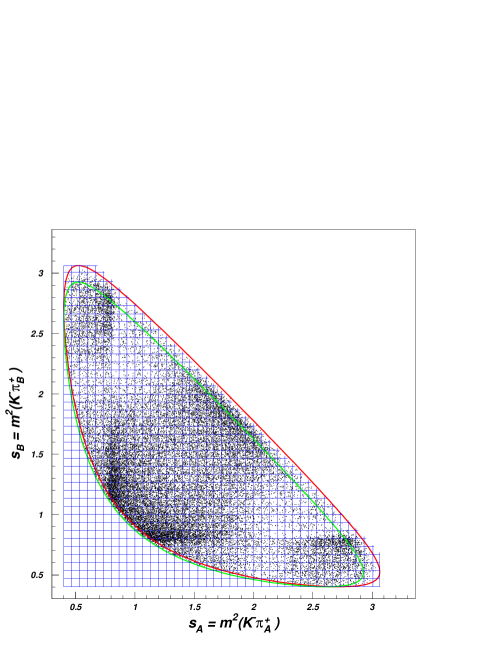
Figure 1: Dalitz plot for $D^{+}\rightarrow K^{-}\pi^{+}_{\scriptscriptstyle A}\pi^{+}_{\scriptscriptstyle B}$ decays. The squared invariant mass $s_{\scriptscriptstyle B}$ of one $K^{-}\pi^{+}$ combination is plotted against $s_{\scriptscriptstyle A}$, the squared invariant mass of the other combination. The plot is symmetrized, each event appearing twice. Lines in both directions indicate values equally spaced in squared effective mass at each of which the $S\hbox{-wave}$ amplitude is determined by the MIPWA described in section III. Kinematic boundaries for the Dalitz plot are drawn for three-body mass values $M=1.810$ and $M=1.890$ $\hbox{GeV}/c^{2}$, between which data are selected for the fits.

II.2 Asymmetry in the $K^{-}\pi^{+}$ System

One of the most striking features of the Dalitz plot is the asymmetry in each $K^{*}(892)$ band. In any given $K^{-}\pi^{+}$ mass slice, a greater density of events exists at one end of that slice than at the other. This asymmetry is also evident in the region closest to the $K^{*}(892)$ peak itself. This is most readily explained by interference with a $K^{-}\pi^{+}$ $S\hbox{-wave}$ component and clearly shows that these data can be used to infer the structure of the $S\hbox{-wave}$ amplitude, provided an adequate modelling of the remainder of the plot is possible.

This asymmetry, $\alpha$, depends on the distribution of the helicity angle, $\theta$, the angle between $K^{-}$ and $\pi^{+}_{\scriptscriptstyle B}$ in the $K^{-}\pi^{+}_{\scriptscriptstyle A}$ rest frame. It is defined hel as

$$\alpha={N_{\cos\theta>0}-N_{\cos\theta<0}\over N_{\cos\theta>0}+N_{\cos\theta<0}}$$ (1)

where $N$ is the efficiency-corrected number of events in the indicated regions of $\cos\theta$. In Fig. 2, $\alpha$ is plotted as a function of the $K^{*}(892)$ Breit-Wigner (BW) phase $\phi_{\scriptscriptstyle BW}=\tan^{-1}[m_{0}\Gamma/(m_{0}^{2}-s)]$, where the peak mass $m_{0}=896.1$ $\hbox{MeV}/c^{2}$ and the mass dependent width $\Gamma=50.7$ $\hbox{MeV}/c^{2}$ at the peak mass. A change in the sign of $\alpha$ occurs when $\phi_{\scriptscriptstyle BW}\sim 56^{\circ}$, at an invariant mass below the $K^{*}(892)$ peak. We note here that, in $K\pi$ elastic scattering Aston et al. (1988), $\alpha$ is observed to reach zero at $\phi_{\scriptscriptstyle BW}\approx 135.5^{{}_{\circ}}$, a mass above the $K^{*}(892)$ peak. Evidently there is a $\sim-79^{{}_{\circ}}$ shift in $s$-$p$ relative phase in this $D^{+}$ decay relative to that observed in $K\pi$ elastic scattering.

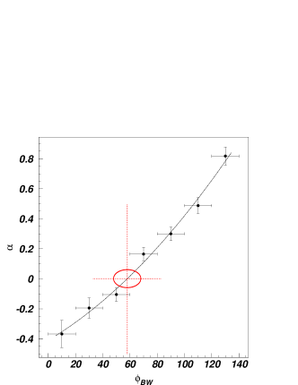
Figure 2: The asymmetry $\alpha$ plotted vs. BW phase $\phi_{\scriptscriptstyle BW}$ for the $K^{*}(892)$. These quantities are described in the text. $\alpha$ becomes zero at $\phi_{\scriptscriptstyle BW}\sim 56$ degrees.

III Formalism

III.1 $K^{-}\pi^{+}$ Partial Wave Expansion

The Dalitz plot in Fig. 1 is described by a complex amplitude Bose-symmetrized with respect to the identical pions $\pi^{+}_{\scriptscriptstyle A}$ and $\pi^{+}_{\scriptscriptstyle B}$:

$${\mathcal{A}}=A(s_{\scriptscriptstyle A},s_{\scriptscriptstyle B})+A(s_{\scriptscriptstyle B},s_{\scriptscriptstyle A}).$$ (2)

Considering the simplest, tree-level quark diagrams, iso-spin $I=1/2$ $K^{-}\pi^{+}$ systems are most likely to be produced. The contribution of the $\pi^{+}\pi^{+}$ amplitude to these decays is not expected to be significant, coming mostly from re-scattering processes. To test this, data are taken from measurements of $\pi^{+}p\rightarrow\pi^{+}\pi^{+}n$ reactions Hoogland et al. (1977) in which the phase of the $\pi^{+}\pi^{+}$ amplitude was found to vary slowly, assuming it to be elastic, from zero at threshold to about $-30^{\circ}$ at 1.45 $\hbox{GeV}/c^{2}$, the upper range of the measurements. No evidence for isospin $I=2$ resonances exists in this range. This amplitude is added to those in model C in Ref.  Aitala et al. (2002). It is found that the $\pi^{+}\pi^{+}$ contribution is, indeed, insignificantly small $(0.7\pm 0.4)$%.

The amplitude $A$ is therefore written as the sum of $K^{-}\pi^{+}$ partial waves labelled by angular momentum quantum number $L$,

$$A(s_{\scriptscriptstyle A},s_{\scriptscriptstyle B}) = \sum_{L=0}^{L_{\hbox{\tiny max}}}(-2pq)^{L}P_{L}(\cos\theta)\times$$ (3)

$${\cal F}_{\scriptscriptstyle D}^{\scriptscriptstyle L}(q,r_{\scriptscriptstyle D})\times C_{L}(s_{\scriptscriptstyle A}),$$

corresponding to production of $K^{-}\pi^{+}$ systems with spin $J=L$ and parity $(-1)^{L}$ in these $D^{+}$ decays. In this analysis, the sum is truncated at $L_{\hbox{\small max}}=2$ since the $D\hbox{-wave}$ $K_{2}^{*}(1430)$, as measured in reference Aitala et al. (2002), contributes only about 0.5% to the decays. This is already small and higher partial-waves are expected to be even further suppressed by the angular momentum barrier. With no way to distinguish $I={1\over 2}$ and $I={3\over 2}$ components in the $K^{-}\pi^{+}$ systems produced, their sum is measured in this paper.

In Eq. (3), $\vec{p}$ and $\vec{q}$ are momenta for the $K^{-}$ and bachelor $\pi^{+}_{\scriptscriptstyle B}$ respectively, in the $K^{-}\pi^{+}_{\scriptscriptstyle A}$ rest frame. The cosine of the helicity angle $\theta$ is then given in terms of the masses $m_{K^{-}}$ ($m_{\pi^{+}}$) and energies $E_{K^{-}}$ ($E_{\pi^{+}}$) of the $K^{-}$ ($\pi^{+}_{\scriptscriptstyle B}$) in the $K^{-}\pi^{+}_{\scriptscriptstyle A}$ rest frame by:

$$\cos\theta = \hat{p}\cdot\hat{q}$$ (4)

$$= {E_{K^{-}}E_{\pi^{+}_{\scriptscriptstyle B}}-\left(s_{\scriptscriptstyle B}-m_{K^{-}}^{2}-m_{\pi^{+}}^{2}\right)/2\over pq}.$$

This is the argument of the Legendre polynomial functions $P_{L}$. ${\cal F}_{\scriptscriptstyle D}^{\scriptscriptstyle L}$ is a form factor for the parent $D$ meson which depends on $q$, $L$ and on the $D$’s effective radius $r=r_{\scriptscriptstyle D}$:

$$\begin{array}[]{lllll}{\cal F}_{\scriptscriptstyle D}^{\scriptscriptstyle 0}&=&e^{-(rq)^{2}/12}&\hbox{scalar}&\\ {\cal F}_{\scriptscriptstyle D}^{\scriptscriptstyle 1}&=&\left[1+(rq)^{2}\right]^{-{1\over 2}}&\hbox{vector}&\\ {\cal F}_{\scriptscriptstyle D}^{\scriptscriptstyle 2}&=&\left[9+3(rq)^{2}+(rq)^{4}\right]^{-{1\over 2}}&\hbox{tensor}&\end{array}$$ (8)

For $L>0$, these form-factors are derived for non-relativistic potential scattering Blatt and Weisskopf (1952). For $L=0$, the Gaussian form in Eq. (8), suggested by Tornqvist Tornqvist (1995) to be a preferred way to describe scalar systems, is used. This form was used also in Ref. Aitala et al. (2002).

The $C_{L}(s_{\scriptscriptstyle A})$ are complex functions, and are the invariant-mass-dependent parts of the respective partial waves. They do not depend on the other Dalitz plot variable $s_{\scriptscriptstyle B}$ and are referred to in this paper as the $K^{-}\pi^{+}$ amplitudes. Provided that interactions between the $K^{-}\pi^{+}_{\scriptscriptstyle A}$ system and the bachelor $\pi^{+}_{\scriptscriptstyle B}$ can be neglected, the $C_{L}(s_{\scriptscriptstyle A})$ are related to the corresponding amplitudes, $T_{L}(s)$ measured in $K^{-}\pi^{+}$ scattering experiments, by

$$C_{L}(s)\equiv|C_{L}(s)|e^{i\phi_{L}(s)} = {\sqrt{s}\over p}{{\cal P}_{L}(s)T_{L}(s)\over p^{L}{\cal F}_{\scriptscriptstyle D}^{\scriptscriptstyle L}},$$ (9)

where ${\cal P}_{L}(s)$, unknown functions, describe the $K^{-}\pi^{+}$ production in each wave in the $D$ decay process Adl . These replace the $K^{-}\pi^{+}$ coupling present in elastic scattering (proportional to the 2-body phase-space factor $\sqrt{s}/p$ and barrier factor $p^{L}$).

The principal goal of this analysis is to measure $C_{0}(s)$, using all higher $L$ contributions to the Dalitz plot as an “interferometer”. This requires a model for $C_{1}(s)$ and $C_{2}(s)$, the reference $P\hbox{-}$ and $D\hbox{-}$ waves.

III.2 The Reference Waves

As in previous analyses, a Breit-Wigner isobar model is used to describe the $P\hbox{-}$ and $D\hbox{-}$waves. Linear combinations of resonant propagators ${\cal W}_{\scriptscriptstyle R}$, one for each of the established resonances $R$ having the appropriate spin, and each with a complex coupling coefficient with respect to $K^{*}(892)$, $B_{\scriptscriptstyle R}=b_{\scriptscriptstyle R}e^{i\beta_{\scriptscriptstyle R}}$, are constructed. Three possible $K^{-}\pi^{+}$ resonances are included in the $P\hbox{-wave}$, but only one in the $D\hbox{-wave}$ in the invariant mass range available to these decays:

$$C_{1}(s) = [{\cal W}_{\scriptscriptstyle K^{*}(892)}(s)+B_{\scriptscriptstyle K_{1}^{*}(1410)}{\cal W}_{\scriptscriptstyle K_{1}^{*}(1410)}(s)+$$ (10)

$$B_{\scriptscriptstyle K_{1}^{*}(1680)}{\cal W}_{\scriptscriptstyle K_{1}^{*}(1680)}(s)]\times{\cal F}_{\scriptscriptstyle R}^{\scriptscriptstyle L}(p,r_{\scriptscriptstyle R}),$$

$$C_{2}(s) = \left[B_{\scriptscriptstyle K_{2}^{*}(1430)}{\cal W}_{\scriptscriptstyle K_{2}^{*}(1430)}(s)\right]\times{\cal F}_{\scriptscriptstyle R}^{\scriptscriptstyle L}(p,r_{\scriptscriptstyle R}).$$ (11)

where ${\cal F}_{\scriptscriptstyle R}^{\scriptscriptstyle L}$ is a form factor for the resonances in the $K^{-}\pi^{+}$ system, required to ensure that the resonant amplitudes vanish for invariant masses far above the pole masses. It is assumed to have the same dependence on center-of-mass momentum and angular momentum as the $D$ form factor ${\cal F}_{\scriptscriptstyle D}^{\scriptscriptstyle L}$, but to depend on a different effective radius $r=r_{\scriptscriptstyle R}$. The coefficients in Eq. (10) have their origin in the $K^{-}\pi^{+}$ production process arising from $D^{+}$ decays, and are therefore treated as unknown parameters in the fits.

Each propagator is assumed to have a Breit-Wigner form defined as:

$${\cal W}_{\scriptscriptstyle R}(s)={1\over m_{\scriptscriptstyle R}^{2}-s-im_{\scriptscriptstyle R}\Gamma(r_{\scriptscriptstyle R},s)},$$ (12)

where $m_{\scriptscriptstyle R}$ and $\Gamma_{\scriptscriptstyle R}$ are the resonance mass and width, and:

$$\Gamma(r_{\scriptscriptstyle R},s)=\Gamma_{\scriptscriptstyle R}\left({m_{\scriptscriptstyle R}\over\sqrt{}s}\right)\left({p\over p_{\scriptscriptstyle R}}\right)^{2L+1}\left[{{\cal F}_{\scriptscriptstyle R}^{\scriptscriptstyle L}(p,r_{\scriptscriptstyle R})\over{\cal F}_{\scriptscriptstyle R}^{\scriptscriptstyle L}(p_{\scriptscriptstyle R},r_{\scriptscriptstyle R})}\right]^{2}$$ (13)

where $p_{\scriptscriptstyle R}$ is the value of $p$ when $s=m_{\scriptscriptstyle R}^{2}$.

III.3 Parametrization of the $S\hbox{-wave}$

The goal is to define the $S\hbox{-wave}$ amplitude making no assumptions about either its scalar meson composition, nor of the form of any $S\hbox{-wave}$ $NR$ terms. To this end, two real parameters are introduced

$$c_{k} = |C_{0}(s_{k})|~{}~{};~{}~{}\gamma_{k}=\phi_{0}(s_{k})$$ (14)

to define the amplitude $C_{0}(s_{k})=c_{k}e^{i\gamma_{k}}$ at each of a set of invariant mass squared values $s=s_{k}~{}(k=1,N_{s})$. A second order spline interpolation is used to define the amplitude between these points $(s_{k},c_{k}e^{i\gamma_{k}})$ Spl . The $c_{K}$ and $\gamma_{k}$ values are treated as model-independent parameters, and are determined by a fit to the data.

To obtain the results in this paper, $N_{s}=40$ equally spaced values of $s_{k}$ are chosen. These are indicated by the lines drawn on the Dalitz plot in Fig. 1. Other sets of values for $s_{k}$ are also used to check the stability of the results obtained.

III.4 Maximum Likelihood Fit

In this analysis, the 3-body mass $M$ is not constrained to be that of the $D^{+}$ meson. The fits are therefore made in three dimensions $(M,s_{\scriptscriptstyle A},s_{\scriptscriptstyle B})$. A normalized, log-likelihood function is defined as

$${\cal L}=\sum_{\hbox{events}}\ln\left[\left(1-\sum_{i=1}^{3}f_{i}\right)P_{s}+\sum_{i=1}^{3}f_{i}P^{i}_{b}\right],$$ (15)

where $P_{s}$ and $P_{b}^{i}$ are the normalized signal and background PDF’s, respectively.

Three backgrounds ($i=1,~{}2,~{}3$), described in Sec. II, are included incoherently in Eq. (15). Each is considered to constitute a fraction $f_{i}$ of the event sample in the selected range $1.850<M<1.890$ $\hbox{GeV}/c^{2}$, and to be described by the PDF:

$$P_{b}^{i} = {Q_{i}(M)\theta_{i}(s_{\scriptscriptstyle A},s_{\scriptscriptstyle B})\over n_{i}}.$$ (16)

This expression has a three-body mass profile $Q_{i}(M)$ and a distribution $\theta_{i}(s_{\scriptscriptstyle A},s_{\scriptscriptstyle B})$, with normalization $n_{i}$, over the Dalitz plot. For the combinatorial background, the PDF is determined by events in a band of $M$ values above the $D^{+}$ peak, while for the $D_{s}$ reflections it is determined from the simulated MC samples.

The signal PDF is

$$P_{s} = {Q_{0}(M)\epsilon(s_{\scriptscriptstyle A},s_{\scriptscriptstyle B})|{\mathcal{A}}(s_{\scriptscriptstyle A},s_{\scriptscriptstyle B})|^{2}\over\int ds_{\scriptscriptstyle A}ds_{\scriptscriptstyle B}dM~{}F(M)\epsilon(s_{\scriptscriptstyle A},s_{\scriptscriptstyle B})|{\mathcal{A}}(s_{\scriptscriptstyle A},s_{\scriptscriptstyle B})|^{2}},$$ (17)

in which $Q_{0}(M)$ describes the shape of the signal component in the $K^{-}\pi^{+}\pi^{+}$ invariant mass spectrum, parametrized as the sum of two Gaussian functions, and $\epsilon(s_{\scriptscriptstyle A},s_{\scriptscriptstyle B})$ is the efficiency for reconstructing these events. The normalization integral extends over the entire Dalitz plot for each $M$ in the selected range.

III.5 Decay Channels and Branching Fractions

The amplitude $A(s_{\scriptscriptstyle A},s_{\scriptscriptstyle B})$ in Eq. (3) can be written as a sum over the $N_{\scriptscriptstyle ch}$ possible decay channels of the $D^{+}$:

$$A(s_{\scriptscriptstyle A},s_{\scriptscriptstyle B})=\sum_{k=1}^{N_{\scriptscriptstyle ch}}A_{k},$$ (18)

where $A_{k}$ is the complex amplitude for the $k^{th}$ decay mode for decay to the $K^{-}\pi^{+}\pi^{+}$ final state through either a resonance, or through the whole set of possible $S\hbox{-wave}$ and $NR$ states. The fraction, $F_{\scriptscriptstyle k}$, is computed for each such mode:

$$F_{\scriptscriptstyle k}={\int_{\scriptscriptstyle DP}|A_{k}|^{2}ds_{\scriptscriptstyle A}ds_{\scriptscriptstyle B}\over\int_{\scriptscriptstyle DP}|\sum_{i}A_{i}|^{2}ds_{\scriptscriptstyle A}ds_{\scriptscriptstyle B}}.$$ (19)

This is the definition most often used in the literature on three body decays. It guarantees that each $F_{\scriptscriptstyle k}$ is positive. Due to interference, however, the $F_{\scriptscriptstyle k}$ do not necessarily sum to unity.

III.6 Parameters, Phases and Constants

The log-likelihood, Eq. (15), is defined by many parameters. By choice, a number of these are held constant in the fits. Parameters for the background models $P^{i}_{b}$ and their fractions $f_{i}$ are determined by studies of data and of MC samples and are fixed. Masses and widths for well-established $P\hbox{-}$ and $D\hbox{-wave}$ resonances are also held constant at values listed in Table 1. These come mostly from the Review of Particle Properties (RPP) publication S. Eidelman et al. (2004). For the $K_{1}^{*}(1680)$ values appropriate for the state with known coupling to $K\pi$ observed in $K\pi$ scattering in the LASS experiment Aston et al. (1988) are used. The form factor radii are fixed at $r_{\scriptscriptstyle D}=5.0$ GeV^-1 and $r_{\scriptscriptstyle R}=1.6$ GeV^-1, values determined in Ref. Aitala et al. (2002) to be those providing the best isobar model description for these data. Isobar coefficients $B_{\scriptscriptstyle R}$ and partial wave amplitude parameters $c_{i}$ and $\gamma_{i}$ are generally allowed to vary.

Table 1: resonance mass $m_{\scriptscriptstyle R}$ and width $\Gamma_{\scriptscriptstyle R}$ values used in the fits described in this paper. With the exception of $K_{1}^{*}(1680)$, parameters are as quoted in Ref. S. Eidelman et al. (2004).

Resonance	$m_{\scriptscriptstyle R}$ ($\hbox{MeV}/c^{2}$)	$\Gamma_{\scriptscriptstyle R}$ ($\hbox{MeV}/c^{2}$)
$K^{*}(892)$	896.1	50.7
$K_{1}^{*}(1410)$	1414.0	232
$K_{1}^{*}(1680)$	1677.0	205
$K_{2}^{*}(1430)$	1432.4	109

Phases are defined relative to the $K^{*}(892)$ resonance. In all fits described here, the coefficient for the $K^{*}(892)$ is taken to be real and of magnitude unity, as explicit in Eq. 10.

Two sources of uncertainty in this method result from the parametrization of the $P\hbox{-wave}$, and from the fact that several local minima in the likelihood function exist. These limitations are discussed in more detail in Appendix A.

IV MIPWA of the $K^{-}\pi^{+}$ $S\hbox{-wave}$

The technique described in Section III is applied to the data shown in the Dalitz plot in Fig. 1. The $P\hbox{-}$ and $D\hbox{-wave}$ amplitudes defined as in Eqs. (10) and (11) are chosen as reference waves. The 40 equally spaced values $s_{k}$, indicated by lines in the figure, are chosen. The $S\hbox{-wave}$ magnitude and phase , $c_{k}$ and $\gamma_{k}$, at each $s_{k}$, and the $P\hbox{-wave}$ and $D\hbox{-wave}$ couplings $B_{\scriptscriptstyle i}$ are all determined by the fit. With all established vector and tensor resonances with masses and widths shown in Table 1, there are 86 free parameters.

It is confirmed that the contribution from $K_{1}^{*}(1410)$ is negligible, as reported in Ref. Aitala et al. (2002), and this is dropped from further consideration. The fit is made with the remaining 84 free parameters. The complex coefficients $B_{\scriptscriptstyle i}$ and the fractions $F_{\scriptscriptstyle i}$ for each of the resonances $i$ included in the $P\hbox{-}$ and $D\hbox{-wave}$s are summarized in Table 2.

Table 2: Fractions, magnitudes and phases for resonant and $S\hbox{-wave}$ components from four fits to decays of $D^{+}$ mesons to $K^{-}\pi^{+}\pi^{+}$ described in the text. Fit labels are “MIPWA” for the fit, described in Sec. IV, where magnitudes and phases for 40 $K^{-}\pi^{+}$ mass slices described in the text are free to vary. Systematic errors are included for this fit. “Isobar” refers to the fit described in Sec. V. The fit labelled as “Elastic” is described in Section VI.

Channel	Fit	Fraction	Amplitude	Phase
		$F_{\scriptscriptstyle\phantom{.}}$%	$b$	$\beta$ (degrees)
$K^{*}(892)\pi^{+}$	MIPWA	11.9$\pm 0.2\pm$ 2.0	1.00 (fixed)	0.0 (fixed)
	Isobar	12.6$\pm$ 1.6	1.00 (fixed)	0.0 (fixed)
	Elastic	12.8$\pm$ 2.0	1.00 (fixed)	0.0 (fixed)
$K_{1}^{*}(1680)\pi^{+}$	MIPWA	1.2$\pm 0.6\pm$ 1.2	1.63$\pm 0.4\pm$ 0.2	42.8$\pm 16.3\pm$ 4.5
	Isobar	2.1$\pm$ 0.4	2.18$\pm$0.2	28.2$\pm$ 7.2
	Elastic	5.0$\pm$ 0.8	3.15$\pm$0.3	17.1$\pm$ 7.5
$K_{2}^{*}(1430)\pi^{+}$	MIPWA	0.2$\pm 0.1\pm$ 0.1	4.31$\pm 1.0\pm$ 1.1	-12.2$\pm 23.7\pm$ 16.8
	Isobar	0.5$\pm$ 0.1	6.50$\pm$0.7	-54.0$\pm$ 7.4
	Elastic	0.3$\pm$ 0.1	4.59$\pm$0.0	-46.9$\pm$12.3
Total $S\hbox{-wave}$:
	MIPWA	78.6$\pm 1.4\pm$ 1.8	EIPWA	EIPWA
	Elastic	79.2$\pm$ 1.1	–	–
$S\hbox{-wave}$ components:
$NR$	Isobar	16.1$\pm$ 5.3	0.60$\pm$0.1	-3.5$\pm$ 9.1
$\kappa\pi^{+}$	Isobar	45.6$\pm$10.7	1.71$\pm$0.2	181.3$\pm$ 8.1
$K_{0}^{*}(1430)\pi^{+}$	Isobar	12.2$\pm$ 1.3	0.52$\pm$0.1	47.0$\pm$ 5.6

loc

The $S\hbox{-wave}$ phases $\gamma_{k}$ ($=\phi_{0}(s_{k})$) and magnitudes $c_{k}$ ($=|C_{0}(s_{k})|$) resulting from the fit are plotted, with error bars, in Figs. 3(a) and (b), respectively. A significant phase variation is observed over the full range of invariant mass, with the strongest variation near the $K_{0}^{*}(1430)$ resonance. The magnitude is largest just above threshold, peaking at about 0.725 $\hbox{GeV}/c^{2}$, above which it falls. A shoulder is seen at the mass of the $K_{0}^{*}(1430)$, after which the magnitude falls sharply to its minimum value just above 1.5 $\hbox{GeV}/c^{2}$.

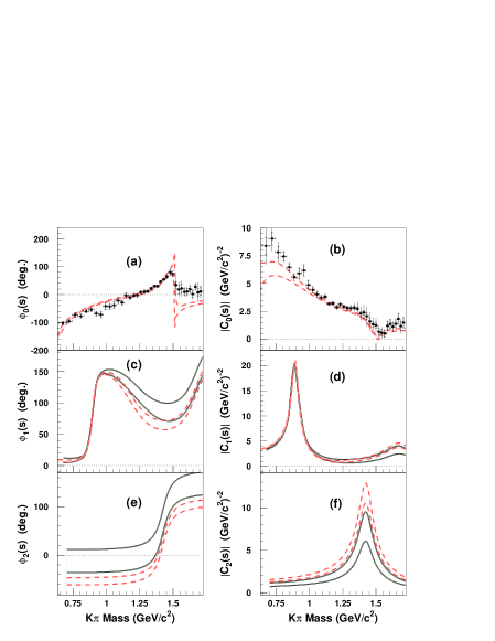
Figure 3: (a) Phases $\gamma_{k}=\phi_{0}(s_{k})$ and (b) magnitudes $c_{k}=|C_{0}(s_{k})|$ of $S\hbox{-wave}$ amplitudes for $K^{-}\pi^{+}$ systems from $D^{+}\rightarrow K^{-}\pi^{+}\pi^{+}$ decays with the amplitude and phase of the $K^{*}(892)$ as reference. Solid circles, with error bars show the values obtained from the MIPWA fit described in the text. The effect of adding systematic uncertainties in quadrature is indicated by extensions on the error bars. The $P\hbox{-wave}$ and $D\hbox{-wave}$ phases are plotted in (c) and (e) and their magnitudes in (d) and (f), respectively. These curves are derived from Eqs. (10) and (11), respectively, evaluated with the parameters and error matrix resulting from the MIPWA. Curves appear as shaded areas bounded by solid line curves representing one standard deviation limits for these quantities. In all plots, the dashed curves show one standard deviation limits for the predictions of the isobar model fit described in Sec. V. These curves are computed in the same way, using Eq. (20) in addition to (10) and (11) with parameters and error matrix from the isobar model fit.

The $S\hbox{-wave}$ magnitudes $c_{k}$ obtained depend on the form used for ${\cal F}_{\scriptscriptstyle D}^{\scriptscriptstyle 0}$ in Eq. (3). The products $c_{k}{\cal F}_{\scriptscriptstyle D}^{\scriptscriptstyle 0}$, and phases $\gamma_{k}$ are, however, independent of ${\cal F}_{\scriptscriptstyle D}^{\scriptscriptstyle 0}$. To simplify future comparisons, values for $c_{k}$, ${\cal F}_{\scriptscriptstyle D}^{\scriptscriptstyle 0}$ and $\gamma_{k}$ for each invariant mass $s_{k}$ are listed, with their uncertainties, in Table 3. In the present analysis, the Gaussian form Tornqvist (1995) in Eq. (8) for $L=0$ has been chosen. The values used for ${\cal F}_{\scriptscriptstyle D}^{\scriptscriptstyle 0}$ at each $s_{k}$ are also listed in Table 3.

Table 3: Magnitude $c$ and phase $\gamma$ of the $K^{-}\pi^{+}$ $S\hbox{-wave}$ amplitude determined, at equally spaced masses, by the MIPWA fit described in the text. The magnitudes assume a real form-factor $F_{\scriptscriptstyle 0}^{\scriptscriptstyle D}$ for the $D^{+}$ meson. Values for this form-factor are given for each mass value in the table. Two further mass values, used in the fit as a result of the finite resolution in 3-body invariant mass, are not included in the table. They lie, respectively, at and above the kinematic limit for $D^{+}$ decay to this final state. Statistical and systematic uncertainties are assigned to each magnitude and phase.

$\sqrt{s}$	$F_{D}^{0}(\sqrt{}s)$	$c$					$\gamma$
$(\hbox{GeV}/c^{2})$		$(\hbox{GeV}/c^{2})^{-2}$					(degrees)
$0.672$	$0.26$	$8.37$	$\pm$	$0.73$	$\pm$	$0.62$	$-102$	$\pm$	$5$	$\pm$	$3$
$0.719$	$0.27$	$9.04$	$\pm$	$0.59$	$\pm$	$0.89$	$-96$	$\pm$	$5$	$\pm$	$3$
$0.764$	$0.29$	$7.82$	$\pm$	$0.54$	$\pm$	$0.89$	$-73$	$\pm$	$9$	$\pm$	$4$
$0.807$	$0.31$	$7.42$	$\pm$	$0.43$	$\pm$	$0.57$	$-77$	$\pm$	$7$	$\pm$	$5$
$0.847$	$0.33$	$6.47$	$\pm$	$0.30$	$\pm$	$0.46$	$-60$	$\pm$	$5$	$\pm$	$6$
$0.885$	$0.34$	$5.57$	$\pm$	$0.31$	$\pm$	$0.07$	$-54$	$\pm$	$6$	$\pm$	$5$
$0.922$	$0.36$	$5.90$	$\pm$	$0.46$	$\pm$	$0.09$	$-68$	$\pm$	$8$	$\pm$	$7$
$0.958$	$0.38$	$6.17$	$\pm$	$0.52$	$\pm$	$0.01$	$-72$	$\pm$	$10$	$\pm$	$9$
$0.992$	$0.40$	$4.87$	$\pm$	$0.35$	$\pm$	$0.19$	$-41$	$\pm$	$12$	$\pm$	$10$
$1.025$	$0.42$	$4.42$	$\pm$	$0.28$	$\pm$	$0.09$	$-43$	$\pm$	$11$	$\pm$	$5$
$1.057$	$0.44$	$4.02$	$\pm$	$0.26$	$\pm$	$0.01$	$-38$	$\pm$	$12$	$\pm$	$5$
$1.088$	$0.46$	$3.74$	$\pm$	$0.19$	$\pm$	$0.11$	$-22$	$\pm$	$10$	$\pm$	$4$
$1.118$	$0.49$	$3.81$	$\pm$	$0.19$	$\pm$	$0.13$	$-29$	$\pm$	$9$	$\pm$	$4$
$1.147$	$0.51$	$3.16$	$\pm$	$0.14$	$\pm$	$0.13$	$-3$	$\pm$	$9$	$\pm$	$4$
$1.176$	$0.53$	$3.21$	$\pm$	$0.15$	$\pm$	$0.13$	$-11$	$\pm$	$7$	$\pm$	$3$
$1.204$	$0.55$	$2.86$	$\pm$	$0.14$	$\pm$	$0.32$	$-3$	$\pm$	$7$	$\pm$	$3$
$1.231$	$0.58$	$3.11$	$\pm$	$0.15$	$\pm$	$0.13$	$-3$	$\pm$	$6$	$\pm$	$2$
$1.258$	$0.60$	$2.92$	$\pm$	$0.15$	$\pm$	$0.24$	$8$	$\pm$	$6$	$\pm$	$3$
$1.284$	$0.62$	$2.80$	$\pm$	$0.16$	$\pm$	$0.18$	$11$	$\pm$	$6$	$\pm$	$2$
$1.310$	$0.65$	$2.77$	$\pm$	$0.17$	$\pm$	$0.12$	$11$	$\pm$	$5$	$\pm$	$2$
$1.335$	$0.67$	$2.83$	$\pm$	$0.17$	$\pm$	$0.20$	$22$	$\pm$	$5$	$\pm$	$2$
$1.360$	$0.69$	$2.73$	$\pm$	$0.19$	$\pm$	$0.31$	$31$	$\pm$	$4$	$\pm$	$2$
$1.384$	$0.71$	$2.29$	$\pm$	$0.20$	$\pm$	$0.25$	$30$	$\pm$	$5$	$\pm$	$2$
$1.408$	$0.74$	$2.38$	$\pm$	$0.23$	$\pm$	$0.01$	$46$	$\pm$	$4$	$\pm$	$2$
$1.431$	$0.76$	$2.05$	$\pm$	$0.28$	$\pm$	$0.08$	$55$	$\pm$	$4$	$\pm$	$2$
$1.454$	$0.78$	$1.59$	$\pm$	$0.25$	$\pm$	$0.07$	$64$	$\pm$	$6$	$\pm$	$4$
$1.477$	$0.80$	$1.33$	$\pm$	$0.24$	$\pm$	$0.01$	$80$	$\pm$	$10$	$\pm$	$4$
$1.499$	$0.82$	$1.23$	$\pm$	$0.24$	$\pm$	$0.01$	$74$	$\pm$	$10$	$\pm$	$4$
$1.522$	$0.84$	$0.66$	$\pm$	$0.30$	$\pm$	$0.27$	$34$	$\pm$	$13$	$\pm$	$21$
$1.543$	$0.86$	$0.57$	$\pm$	$0.29$	$\pm$	$0.11$	$18$	$\pm$	$16$	$\pm$	$22$
$1.565$	$0.88$	$0.50$	$\pm$	$0.30$	$\pm$	$0.01$	$22$	$\pm$	$17$	$\pm$	$23$
$1.586$	$0.90$	$1.18$	$\pm$	$0.35$	$\pm$	$0.01$	$10$	$\pm$	$10$	$\pm$	$14$
$1.607$	$0.92$	$1.35$	$\pm$	$0.37$	$\pm$	$0.18$	$11$	$\pm$	$10$	$\pm$	$14$
$1.627$	$0.93$	$1.11$	$\pm$	$0.37$	$\pm$	$0.14$	$19$	$\pm$	$10$	$\pm$	$14$
$1.648$	$0.95$	$1.37$	$\pm$	$0.35$	$\pm$	$0.01$	$2$	$\pm$	$10$	$\pm$	$14$
$1.668$	$0.96$	$1.82$	$\pm$	$0.43$	$\pm$	$0.01$	$28$	$\pm$	$8$	$\pm$	$12$
$1.687$	$0.98$	$1.16$	$\pm$	$0.40$	$\pm$	$0.84$	$8$	$\pm$	$14$	$\pm$	$34$
$1.707$	$0.99$	$1.47$	$\pm$	$0.46$	$\pm$	$0.01$	$11$	$\pm$	$14$	$\pm$	$21$

The magnitudes $|C_{L}(s)|$ and phases $\phi_{L}(s)$ for the $P\hbox{-}$ and $D\hbox{-wave}$ amplitudes $C_{L}(s)~{}~{}(L=1,2)$ are computed from Eqs. (10) and (11), using parameters for this fit from Tables 1 and 2. Uncertainties in these quantities are also computed, using the full error matrix from the fit. Values, at each $s$, plus or minus one standard deviation are then plotted as solid curves, with shading between them, in Fig. 3. The $P\hbox{-wave}$ phase and magnitude are shown, respectively, in Figs. 3(c) and (d), and those for the $D\hbox{-wave}$ in (e) and (f).

To compare the fit with the data, MC simulated samples of events are produced in the three-dimensional space in which the fits are made. Events are generated with the distribution predicted from the signal and background PDF’s defined in Eq. (15). Parameter values from Tables 2 and 3, and the measured event reconstruction efficiency $\epsilon(s_{\scriptscriptstyle A},s_{\scriptscriptstyle B})$, are used in the simulation. These events are projected onto the two-dimensional Dalitz plot, and its one-dimensional invariant mass plots. Data are then overlayed for comparison. These plots are shown in Fig. 4. As a further comparison, the distributions of the helicity angle $\theta$ in the $K^{-}\pi^{+}$ systems predicted by the fit are compared to the data. Fig. 5 shows moments for this angle, $(dN/dm)\langle P_{L}(\cos\theta)\rangle$, uncorrected for acceptance.

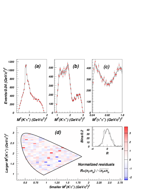
Figure 4: Comparison between MIPWA fit and data for $D^{+}\rightarrow K^{-}\pi^{+}\pi^{+}$ decays. For each event, the distributions of (a) the smaller $K^{-}\pi^{+}$, (b) the larger $K^{-}\pi^{+}$ and (c) the $\pi^{+}\pi^{+}$ squared invariant masses are plotted as points with error bars. Results of the fit (solid histogram) are superimposed. (d) The Dalitz plot folded about the axis of symmetry resulting from the identity of the two $\pi^{+}$ mesons. The quantity plotted is the normalized residual $(n_{f}-n_{0})/\sqrt{n_{f}+n_{o}}$ defined in the text. The histogram is the distribution of normalized residual values and the curve is a Gaussian fit to this having mean $-0.015\pm 0.039$ and standard deviation $0.93\pm 0.04$.

Figure 5: Moments of the $K^{-}\pi^{+}$ helicity angle $\theta$ for the MIPWA fit. In each figure, events are plotted in bins of $K^{-}\pi^{+}$ invariant mass with weights equal to $P_{L}(\cos\theta)$ as indicated. Two combinations are plotted for each $K^{-}\pi^{+}\pi^{+}$ candidate. Data are represented as points with error bars. Events are not weighted for their estimated efficiency. The MC events, treated the same way, are used to show the expectation for these moments from the fit, and are shown as solid histograms.

Qualitatively, agreement between the fit and the data is very good. Quantitative comparison is made using the observed distribution of events on the Dalitz plot. The plot is divided into rectangular bins. For each of these, the normalized residual, $(n_{f}-n_{o})/\sigma$, where $n_{o}$ is the number of events observed, $n_{f}$ is the number predicted by the fit and $\sigma=\sqrt{n_{f}+n_{o}}$ is the uncertainty in $n_{f}-n_{o}$, is computed. The expected population in each bin, $n_{f}$, is computed by numerical integration of the PDF in Eq. 15. Neighboring bins are combined, where necessary, to ensure that $n_{f}\geq 10$. The normalized residuals, plotted as an inset in Fig. 4(d), are combined to obtain $\chi^{2}/\hbox{\small NDF}$ where NDF is the number of bins less the number of free parameters in the fit. These values, and the probability for obtaining them, are tabulated with the optimum log-likelihood value from the fit, given in Table 4.

Table 4: Likelihood values for fits to the E791 $K^{-}\pi^{+}$ system from $D^{+}\rightarrow K^{-}\pi^{+}\pi^{+}$ decays. The fits are described in the text and are labelled the same way as in Table 2.

Model	$\ln({\cal L})$	Number of	$NDF$	$\chi^{2}/NDF$	Probability
		Variables
MIPWA fit	36121	86	277	1.00	47.8%
Isobar	36072	16	412	1.08	13.2%
Elastic	36092	44	300	0.99	54.9%
Unitary	36004	44	195	2.68	$\sim 0$

V Comparison with an isobar model fit

It is interesting to compare the results from the MIPWA with those reported in Ref. Aitala et al. (2002) which came from a Breit-Wigner isobar model fit. In this fit, the $S\hbox{-wave}$ was modelled as a sum of isobars with Breit-Wigner propagators for the $K_{0}^{*}(1430)$ resonance, and another $\kappa$ state. An “NR” term, defined as a constant everywhere on the Dalitz plot, was also included in the $S\hbox{-wave}$

$$C_{1}(s) = \left[NR+B_{\scriptscriptstyle\kappa}{\cal W}_{\scriptscriptstyle\kappa}(s)+B_{\scriptscriptstyle K_{0}^{*}(1430)}{\cal W}_{\scriptscriptstyle K_{0}^{*}(1430)}(s)\right]$$ (20)

$$\times{\cal F}_{\scriptscriptstyle R}^{\scriptscriptstyle L}(p,r_{\scriptscriptstyle R}).$$

The $P\hbox{-}$ and $D\hbox{-wave}$s were defined as in Eqs. (10) and (11).

For purposes of comparison, this fit is made again, exactly as before, except that the resonance parameters indicated in Table 1 are used to replace those from Ref. Aitala et al. (2002). Both the $\kappa$ and $K_{0}^{*}(1430)$ isobars included in the $S\hbox{-wave}$ in Eq. (20) have masses and widths that are allowed to vary. The phase convention is defined, as before, by Eq. (10). As found in Ref. Aitala et al. (2002), the amplitude and fraction for $K_{1}^{*}(1410)$ are negligibly small. This resonance is, therefore, also omitted from this fit which is labelled the “isobar fit”. The couplings and fractions obtained are summarized in Table 2. It is seen that the $NR$ term contributes modestly to the decays in this model. Its presence is, however, important as it interferes with the $\kappa$, destructively at $K^{-}\pi^{+}$ threshold, not at all at 780 $\hbox{MeV}/c^{2}$, and constructively at higher mass. Without the $NR$ term, the $S\hbox{-wave}$ form does not fit the data well. All these results, including Breit-Wigner masses and widths obtained for the $S\hbox{-wave}$ states, agree well, within uncertainties, with those in Ref. Aitala et al. (2002).

Amplitudes from this fit are plotted in Figs. 3(a)-(f) where they may be compared with the MIPWA results. As for the MIPWA, Eqs. (10) and (11) are used, this time with parameters for the isobar fit in Table 2 to compute the magnitudes $|C_{L}(s)|$ and phases $\phi_{L}(s)$ for the $P\hbox{-}$ and $D\hbox{-wave}$, respectively, for $L=0$ and $1$. Eq. (20) is used in the same way to compute the $S\hbox{-wave}$ amplitude. Uncertainties in magnitudes and in phases are computed using the full error matrix from the isobar fit and values at each $s$, plus or minus one standard deviation, are plotted as dashed curves, with shading between them, in the appropriate entries in Fig. 3.

The isobar fit constrains the $S\hbox{-wave}$ magnitude and phase to assume the functional forms specified in Eq. (20) while the MIPWA allows them complete freedom. Because of the additional degrees of freedom, the latter is therefore able to achieve a better description of the data by a combination of shifts in the $P\hbox{-}$ and $D\hbox{-wave}$ parameters, and in the $(c_{k},\gamma_{k})$ values for the $S\hbox{-wave}$. The results presented in Figs. 3(a)-(f), and in Table 2, illustrate this. Small differences between the fits in parameters for $K_{1}^{*}(1680)$ and $K_{2}^{*}(1430)$ result in relatively large shifts in the curves shown in Figs. 3(c)-(f). These changes propagate to the $S\hbox{-wave}$.

The shapes predicted by both fits for the $S\hbox{-wave}$ phase and magnitude, are shown in Figs. 3(a) and (b). Some differences are seen in magnitudes from $K^{-}\pi^{+}$ threshold up to about 900 $\hbox{MeV}/c^{2}$, and in both phase and magnitude above the $K_{0}^{*}(1430)$ resonance. These effects are correlated with one another and with the differences in the $P\hbox{-}$ and $D\hbox{-wave}$s noted above. Similar effects are observed in tests made on a large number of MC samples, with sizes similar to that of the data. Approximately 15% of these samples, generated with the distribution predicted by the isobar fit, give MIPWA results with similar shifts in $P\hbox{-}$ and $D\hbox{-wave}$ parameters, and in the associated differences in $S\hbox{-wave}$ observed in the data. The MC tests are discussed in Appendix A.

The significance of any differences between amplitudes obtained in the two fits is evaluated by comparing their abilities to describe distributions of kinematic quantities observed in the data. Plots similar to those in Figs. 4 and 5 are made showing similar, excellent agreement between fit and data. Using the method described in the previous Section, the distribution observed on the Dalitz plot is compared, quantitatively, with that described by the isobar fit results. A value for $\chi^{2}/\hbox{\small NDF}=1.08$ is obtained, and can be compared with $\chi^{2}/\hbox{\small NDF}=1.00$ for the MIPWA. These results are included in Table 4. Differences between the two fits in predicted populations of bins in the Dalitz plot are all less than their statistical uncertainties. It is evident that both MIPWA and isobar fits are good and that no statistically significant distinction between these two descriptions of the data can be drawn with a sample of this size.

VI Comparison of MIPWA with Elastic Scattering

It is interesting to compare the amplitudes $C_{L}(s)$ defined in Sec. III and measured in Sec. IV with those from $K^{-}\pi^{+}$ scattering, $T_{L}(s)$. The relationship between $C_{L}$ and $T_{L}$ is given by Eq. (9). If the $K^{-}\pi^{+}_{\scriptscriptstyle A}$ systems produced in $D^{+}\rightarrow K^{-}\pi^{+}_{\scriptscriptstyle A}\pi^{+}_{\scriptscriptstyle B}$ decays do not interact with the bachelor $\pi^{+}_{\scriptscriptstyle B}$, then the factor ${\cal P}_{L}(s)$ describes the production of $K^{-}\pi^{+}$ as a function of $s$ from these decays. Also, under the same assumptions, the Watson theorem Watson (1952) requires that, in the $s$ range where $K^{-}\pi^{+}$ scattering is purely elastic, ${\cal P}_{L}(s)$ for each partial wave labelled by $L$ and by iso-spin $I$, should carry no $s$-dependent phase. In other words, $\phi_{L}$, the phase of $C_{L}(s)$ for each partial wave, should differ, at most, by a constant relative to that of the corresponding elastic scattering amplitude $T_{L}(s)$. The magnitudes $|C_{L}(s)|$ and $|T_{L}(s)|$ could differ, however, due to any $s$-dependence of the production rate of $K^{-}\pi^{+}$ systems in $D^{+}$ decay.

The validity of the Watson theorem therefore relies on the assumption that no final state scattering between $(K^{-}\pi^{+}_{\scriptscriptstyle A})$ and $\pi^{+}_{\scriptscriptstyle B}$ occurs. This assumption, for decays such as those studied here in which the final state consists of strongly interacting particles, has often been assumed to hold. However, it has never been objectively tested. The MIPWA results from the present data provide, therefore, an interesting opportunity to make such a test, and also to examine the form for the production factor ${\cal P}_{L}(s)$.

VI.1 $K^{-}\pi^{+}$ Scattering

In the $S\hbox{-wave}$, below $K\eta^{\prime}$ threshold at 1.454 $\hbox{GeV}/c^{2}$, $K^{-}\pi^{+}$ scattering in both the isospin $I={1\over 2}$ and $I={3\over 2}$ $K\pi$ amplitudes is predominantly elastic. Scattering into $K\eta$ at a lower threshold is strongly suppressed by the $SU(3)_{\hbox{\tiny flavor}}$ coupling to this channel. This has been confirmed by the LASS collaboration in energy independent measurements of partial wave amplitudes for $K^{-}\pi^{+}$ scattering through, and beyond this range Aston et al. (1988). $I={1\over 2}$ components of $S\hbox{-}$, $P\hbox{-}$ and $D\hbox{-wave}$s were extracted from the total using measurements of the $I={3\over 2}$ scattering from $K^{+}\rightarrow K^{+}\pi^{+}n$ data Ref. Estabrooks et al. (1978). Scattering in higher angular momentum waves can become inelastic at the lower $K\pi\pi$ threshold. It was observed, however, that, in the LASS data, $P\hbox{-wave}$ scattering remained elastic up to approximately 1050 $\hbox{MeV}/c^{2}$. For the $D\hbox{-wave}$, no significant elastic scattering was observed.

In the elastic region, the $I={1\over 2}$ component of the $S\hbox{-wave}$ $K^{-}\pi^{+}$ amplitude was fit, by the LASS collaboration, to a unitary form

$$T_{0}(s) = \sin[\gamma(s)-\gamma_{0}]e^{i[\gamma(s)-\gamma_{0}]},$$ (21)

where the phase $\gamma=\gamma_{\scriptscriptstyle R}+\gamma_{B}+\gamma_{0}$ is made up from three contributions:

$$\begin{array}[]{lcl}\cot\gamma_{\scriptscriptstyle B}&=&{1\over pa}+{1\over 2}bp,\\ \cot\gamma_{\scriptscriptstyle R}&=&{m_{\scriptscriptstyle R}^{2}-s\over m_{\scriptscriptstyle R}\Gamma(r_{\scriptscriptstyle R},s)},\\ \gamma_{0}&=&0~{}~{}\hbox{(arbitrary offset)}.\end{array}$$ (25)

The first is a non-resonant contribution defined by a scattering length $a$ and an effective range $b$. The second contribution $\gamma_{\scriptscriptstyle R}$ has parameters $m_{\scriptscriptstyle R}$ and $\Gamma_{\scriptscriptstyle R}$, the mass and width of the $K_{0}^{*}(1430)$ resonance. In the LASS analysis, the arbitrary phase $\gamma_{0}$ was set to zero. The $I={1\over 2}$ $P\hbox{-wave}$ and $D\hbox{-wave}$ amplitudes measured by LASS were found to be significant in this invariant mass range.

VI.2 Test of the Watson Theorem

In Figs. 6(a)-(c), direct comparisons are made, respectively, between the $S\hbox{-}$, $P\hbox{-}$ and $D\hbox{-wave}$ phases determined by the MIPWA fit to data from this experiment and the $I={1\over 2}$ data from LASS. The $S\hbox{-wave}$ phase measurements, and the curves for the $P\hbox{-}$ and $D\hbox{-wave}$s resulting from the MIPWA, previously shown in Fig. 3, are plotted, respectively, in Figs. 6(a), (b) and (c). The LASS measurements are superimposed, as $\times$’s with error bars, in the appropriate places in the figure.

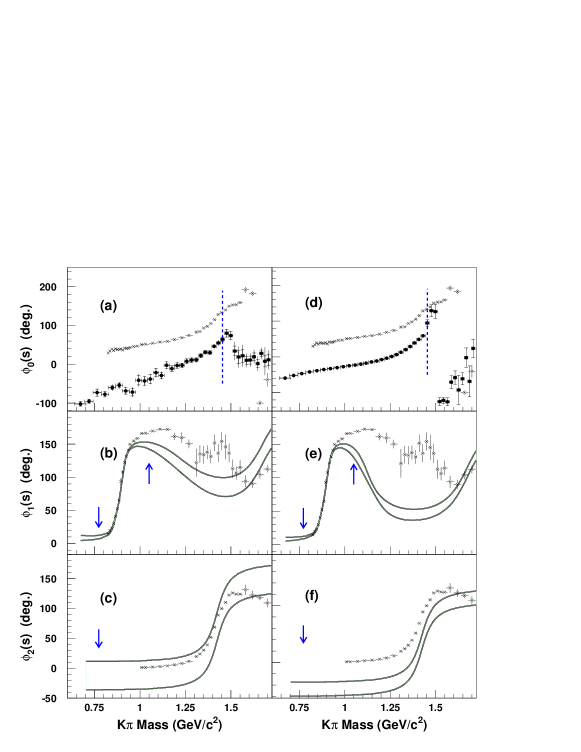
Figure 6: Plots show comparisons between results obtained from the MIPWA, described in Sec. IV, for phases of the (a) $S\hbox{-wave}$, (b) $P\hbox{-wave}$ and (c) $D\hbox{-wave}$ $K^{-}\pi^{+}$ scattering amplitudes with measurements made by the LASS collaboration Aston et al. (1988). Solid circles in (a) are the phases $\gamma_{k}$ obtained at each invariant mass $s_{k}$ from the MIPWA. The vertical dashed line at the $K\eta^{\prime}$ threshold (1454 $\hbox{MeV}/c^{2}$) indicates the upper limit of the range where $K^{-}\pi^{+}$ scattering is predominantly elastic in the $S\hbox{-wave}$. Solid curves in (b) and (c) enclose the zones within one standard deviation of the MIPWA $P\hbox{-}$ and $D\hbox{-wave}$s, computed as described in Sec. IV. Arrows indicate the position of the $K\pi\pi$ threshold, at which $K^{-}\pi^{+}$ scattering in the $P\hbox{-}$ and $D\hbox{-wave}$s can become inelastic. In (b) a further arrow at $1050$ $\hbox{MeV}/c^{2}$ indicates the approximate invariant mass at which the $P\hbox{-wave}$ data from Ref. Aston et al. (1988) were observed to become inelastic. In (d)-(f) the results from the “elastic fit” are shown in place of those from the MIPWA. In all plots $I={1\over 2}$ measurements from the LASS experiment of phases for $K^{-}\pi^{+}$ scattering in these waves are shown as $\times$’s with error bars indicating statistical uncertainties.

An obvious feature in the comparison is the overall shift in phase of the $S\hbox{-wave}$ in these data relative to that in the LASS measurements. This feature is also evident from the examination of the $K^{-}\pi^{+}$ asymmetry in the Dalitz plot reported in Sec. II. Another feature of the $S\hbox{-wave}$ comparison is that, for invariant masses near $K\pi$ threshold, the phases for the two sets of data show a somewhat different dependence on $s$.

The $P\hbox{-wave}$s also differ in the mass range from the $K^{*}(892)$ peak, through the region where LASS observed $K_{1}^{*}(1410)$ scattering to become inelastic, at approximately 1050 $\hbox{MeV}/c^{2}$. This difference may arise, in part, from the parametrization of this wave given in Eq. 10. With more than one resonance described by Breit-Wigner propagators, this may not be unitary. The phase measured in the $D\hbox{-wave}$ in this experiment agrees well with that measured by LASS. However, as verified by the LASS data, the scattering in this wave is no longer elastic beyond $K^{*}(892)\pi^{+}$ threshold.

The observed shift in $S\hbox{-wave}$ phase and difference in slope, and the difference in $P\hbox{-wave}$ phase behaviour evidenced in Figs. 6(a)-(c) do not conform to the precise expectations of the Watson theorem.

VI.3 Fit with LASS Model for $S\hbox{-wave}$ Phase

Some of the discrepancies noted above could arise from the modelling of the $P\hbox{-wave}$. A different model could result in a different dependence on $s$ of the $S\hbox{-wave}$ measured here. To judge the significance of the observed discrepancies, therefore, a fit is made to the data in which the $S\hbox{-wave}$ phase is constrained to precisely follow the LASS parametrization in Eqs. (21-25) for invariant masses below $K\eta^{\prime}$ threshold. The mass and width of the $K_{0}^{*}(1430)$ and the parameters $a$ and $b$ are required to assume the values obtained by LASS. However, the overall phase $\gamma_{0}$, all phases above $K\eta^{\prime}$ threshold, all magnitudes throughout the entire range of $s$, and the complex couplings for $P\hbox{-}$ and $D\hbox{-wave}$s are determined by the fit.

This is labelled as the “elastic fit”. A value $\gamma_{0}=(-74.4\pm 1.8\pm 1.0)^{\circ}$ is obtained. The isobar couplings and resonance fractions obtained are listed in Table 2. The $K_{1}^{*}(1680)$ resonance has a more significant contribution to this fit than in the MIPWA.

The phases obtained for the three partial waves from the elastic fit are compared, in Figs. 6(d)-(f), with those measured in the LASS experiment. The comparison is shown in the same way as in Figs. 6(a)-(c) for the MIPWA fit. The shape of the $S\hbox{-wave}$ phase is, as required in this fit, in perfect agreement with the LASS results. The large offset in overall phase, $\gamma_{0}$ does, however persist. Additionally, both the $P\hbox{-}$ and $D\hbox{-wave}$ phases now show larger differences than before. The $D\hbox{-wave}$ phase shifts by $\sim 50^{{}_{\circ}}$, and the $P\hbox{-wave}$ phase shows significant differences in the region between the $K^{*}(892)$ peak and the effective limit of elastic scattering at $\sim 1050$ $\hbox{MeV}/c^{2}$.

This fit provides another excellent description of the data, with $\chi^{2}/\hbox{\small NDF}=0.99$ and probability 55%, as recorded in Table 4. This is comparable with both the isobar and MIPWA fits. However, if these observations are predominantly of production of $I={1\over 2}$ $K^{-}\pi^{+}$ systems, the phase variation required by the Watson theorem, is not observed in these data.

VI.4 Production Rate for the $K^{-}\pi^{+}$ System

For purely elastic scattering, the $T_{L}$ amplitudes are required to be unitary, as given by Eq. (21). Introducing this into Eq. (9) leads to

$$C_{L}(s) = \left({\sqrt{s}\over p}\right)\left({{\cal P}_{L}(s)\over p^{L}{\cal F}_{\scriptscriptstyle D}^{\scriptscriptstyle L}}\right)\times$$ (26)

$$\sin[\gamma(s)-\gamma_{0}]e^{i[\gamma(s)-\gamma_{0}]}.$$

For $$L=0$$

$$|{\cal P}_{0}(s)| = \left({p\over\sqrt{s}}\right)\left({{\cal F}_{\scriptscriptstyle D}^{\scriptscriptstyle 0}|C_{0}(s)|\over\sin[\gamma(s)-\gamma_{0}]}\right)$$ (27)

Structure in the $s$-dependence of the $S\hbox{-wave}$ magnitude, $C_{0}(s)$ can thus come either from the phase $\gamma(s)$, from ${\cal P}_{0}(s)$, or from both. It is of interest to study these possibilities, and to see if the data can be described by a unitary amplitude, in which ${\cal P}_{0}(s)$ would be independent of $s$.

The data from the MIPWA are examined to see if the $S\hbox{-wave}$ can be described by a unitary amplitude, such as that given in Eq. (26). Setting $L=0$ and ${\cal P}_{0}(s)=P$ (a constant), a value for $\gamma_{0}$ is determined by minimizing the quantity

$$\chi^{2}=\sum_{k=1}^{N_{K\eta^{\prime}}}\left({|{\cal P}_{0}(s_{k})|-P\over\sigma({\cal P}_{0})}\right)^{2},$$ (28)

where $|{\cal P}_{0}(s_{k})|$ are computed from Eq. (27), for the values of $S\hbox{-wave}$ amplitude, $C_{0}(s_{k})=c_{k}e^{i\gamma_{k}}$, determined by the MIPWA fit, and $\sigma({\cal P}_{0})$ are the associated uncertainties. The summation in Eq. (28) is made only for the $N_{K\eta^{\prime}}$ values of $s_{k}$ up to the $K^{-}\eta^{\prime}$ threshold. The value $\gamma_{0}=(-123.3\pm 3.9)^{\circ}$ is obtained, with $P=0.74\pm 0.01~{}(\hbox{GeV}/c^{2})^{-2}$. Fig. 3(a) shows that this value for $\gamma_{0}$ is approximately equal to the measured $S\hbox{-wave}$ phase at $K^{-}\pi^{+}$ threshold, consistent with the physical meaning of this parameter in the formulation in Eq. (26).

Inserting this value for $\gamma_{0}$ into Eq. (27), the quantities $|{\cal P}_{0}{s_{k}}|$ are plotted in Fig. 7. The solid, horizontal line indicates the value for $P$ obtained from the fit. The points are seen to lie close to this line, showing very little dependence on $s$ in the invariant mass range from $K^{-}\pi^{+}$ threshold up to about 1.25 $\hbox{GeV}/c^{2}$. From 1.25 to 1.5 $\hbox{GeV}/c^{2}$, strong variation is observed. In this region, as seen in Fig. 3(a), the value of $\sin(\gamma-\gamma_{0})$, which appears in the denominator of Eq. (27), is approximately zero.

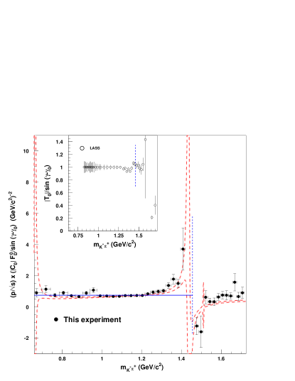
Figure 7: The quantities $p/\sqrt{(}s_{k})\times|C_{0}(s_{k})|\times{\cal F}_{\scriptscriptstyle D}^{\scriptscriptstyle 0}/\sin(\gamma_{k}-\gamma_{0})$ plotted as solid circles for each point obtained for the $S\hbox{-wave}$ amplitude in the MIPWA fit described in Sec. IV. Three points between 1400 and 1450 $\hbox{MeV}/c^{2}$ are omitted from the plot as their values for $\sin(\gamma_{k}-\gamma_{0})$ are very small. Their values are either off-scale or their errors extremely large. The region between the dashed lines shows the one standard deviation limits of this quantity for the $S\hbox{-wave}$ amplitude obtained from the isobar fit. The inset shows, as small open circles, the quantities $|T_{0}(s)|/\sin(\gamma_{\scriptscriptstyle B}+\gamma_{\scriptscriptstyle R})$ taken from the LASS experiment. The $K\eta^{\prime}$ threshold is indicated by dashed, vertical lines in both plots.

Also shown in Fig. 7 is $|{\cal P}_{0}(s)|$ for the isobar fit. The region between dashed lines corresponds to the one standard deviation limits for this quantity, computed from Eq. (27) with the same value of $\gamma_{0}$ as used above. Values for magnitude and phase of the $S\hbox{-wave}$ amplitude, and their statistical uncertainties, are computed from Eq. (20) with parameters and error matrix from this fit. The behaviour of $|{\cal P}_{0}(s)|$ derived from the isobar model fit matches that observed in the MIPWA points well.

The inset in Fig. 7 shows the corresponding quantities $|T_{0}(s)|/\sin(\gamma_{\scriptscriptstyle B}+\gamma_{\scriptscriptstyle R})$ for the points measured for $K^{-}\pi^{+}$ scattering in the LASS experiment. From Eqs. (21) and (25) it is seen that this is expected, in the range up to $K^{-}\eta^{\prime}$ threshold, to be unity. It is seen that this condition is met by the LASS data.

It is concluded that the factor $|{\cal P}_{0}(s)|$ in Eq. (27) that describes production (and possible re-scattering) for $K^{-}\pi^{+}$ systems in the $D^{+}$ decays examined here, shows little dependence on $s$ up to about 1.25 $\hbox{GeV}/c^{2}$. At this point, a significant dependence on $s$ is seen. This behaviour is qualitatively different from elastic scattering.

VII Systematic uncertainties

The major source of systematic uncertainty in the MIPWA results arises from the difficulty, with a sample of this size, of reliably characterizing the structures, other than the $K^{*}(892)$ resonance, in the reference waves. To estimate this effect, a large number of samples of MC events, each of which is of a size similar to the data ($\sim 15K$ events) reported here, are examined. These are generated with the parameters determined by the isobar model fit described in Sec. V, with the backgrounds best matched to the E791 data. Each sample is subjected to a MIPWA fit, and the differences between generated and fitted values for $S\hbox{-wave}$ magnitude and phase at each of the 40 invariant masses are examined. For most samples, fits obtained match the isobar model well. Variations in the significance of the $K_{1}^{*}(1680)$ and $K_{2}^{*}(1430)$ sometimes lead to variations in the reference waves that propagate to distortions in the $S\hbox{-wave}$ solutions found. These tests provide estimates of systematic uncertainties for the $S\hbox{-wave}$ magnitudes that range from $\sim~{}50$% of the statistical uncertainty, for invariant masses below 800 $\hbox{MeV}/c^{2}$, to an insignificant level for higher masses. For the $S\hbox{-wave}$ phases, the systematic uncertainties are found to average $\sim 72$% of the statistical uncertainty.

The second largest uncertainty arises from the smearing of events near the high mass boundary of the Dalitz plot which results from the resolution in three-body mass $M$. This directly affects part of the $K_{1}^{*}(1680)$ band. Events in the region of $M$ closest to the $D^{+}$ mass are fitted separately, and the results compared with that from the larger sample. Average systematic uncertainties arising from the effects of smearing are determined to be 7% of the statistical uncertainties for magnitudes and 14% of the statistical uncertainties for phases. Other effects are studied. These include the uncertainty in precise knowledge of the background level, variations in the values assumed for the radii $r_{\scriptscriptstyle R}$ and $r_{\scriptscriptstyle D}$, or for the mass and width for the $K_{1}^{*}(1680)$ resonance. All these other effects are found to be small.

A further source of systematic uncertainty arises from variations in the presumed resonant composition of the $K^{-}\pi^{+}$ $P\hbox{-}$ and $D\hbox{-wave}$s. The $K^{*}(892)$ resonance obviously contributes, and it is clear that a contribution from a higher resonance, must also exist. What is less clear is the identity of this resonance - $K_{2}^{*}(1430)$, $K_{1}^{*}(1680)$ or for $K_{1}^{*}(1410)$. Fits are made with various combinations of these resonances. It is found that systematic shifts are negligibly small in most cases. Fits where only $K^{*}(892)$ and $K_{2}^{*}(1430)$ are included do lead to shifts comparable to the statistical uncertainties in the lowest five magnitudes. At higher invariant masses, the effects become smaller. The phases are almost unchanged, however.

These uncertainties are combined in quadrature and listed for each invariant mass in Table 3, and for the reference wave parameters in the MIPWA fit in Table 2.

VIII Summary and conclusions

A Model-Independent Partial Wave Analysis (MIPWA) of the $S\hbox{-wave}$ $K^{-}\pi^{+}$ system is made using the three body decay $D^{+}\rightarrow K^{-}\pi^{+}\pi^{+}$. This is the first time such a technique has been used in studying heavy quark meson decays, and new information on the $K^{-}\pi^{+}$ system is obtained, including the invariant mass range below 825 $\hbox{MeV}/c^{2}$. The isospin $I$ of the $S\hbox{-wave}$ measured is unknown, and the $P\hbox{-}$ and $D\hbox{-wave}$s are assumed to be $I={1\over 2}$. It is possible to modify these assumptions, provided independent information on the $I={3\over 2}$ components is available. The method does not assume any form for the energy dependence of the $S\hbox{-wave}$. However, it does so for the $P\hbox{-}$ and $D\hbox{-}$ reference waves. The $P\hbox{-wave}$ is described as the sum of a Breit-Wigner propagator term for the $K^{*}(892)$ resonance, and a similar term, with a complex coefficient, for the $K_{1}^{*}(1680)$. The $K_{1}^{*}(1410)$ is found to have an insignificant contribution to the decays, and is omitted from this wave. The $D\hbox{-wave}$ is described by a single Breit-Wigner term for the $K_{2}^{*}(1430)$ resonance, with a further complex coefficient. The results obtained in Fig. 3 and Table 3 depend on the accuracy of this description of the reference waves.

Results of the MIPWA are compared with a description of the $S\hbox{-wave}$ amplitude that includes Breit-Wigner $\kappa$, $K_{0}^{*}(1430)$ isobars and a constant, non-resonant ($NR$) term similar to the description used in Ref. Aitala et al. (2002). At the statistical level of this experiment, differences between the MIPWA and the isobar-model result are not found to be significant, and both provide good descriptions of the data. A closer examination of the phase behavior in the low mass region below $825$ $\hbox{MeV}/c^{2}$, the limit of measurements of $K^{-}\pi^{+}$ elastic scattering from the LASS experiment Aston et al. (1988), is of considerable importance to the further understanding of scalar spectroscopy. The data here provide new information in this region, but the error bars are large compared to those typical for the LASS data. We note that, since these data became available, a fit that includes requirements of chiral perturbation theory has been made together with the LASS $I=1/2$ measurements and data from $J/\psi\rightarrow K^{*}(892)K^{-}\pi^{+}$. This fit finds a $\kappa$ pole at $(740^{+30}_{-55})-i(342\pm 60)$ $\hbox{MeV}/c^{2}$Bugg (2005). A full understanding of scalar K* spectroscopy may, nevertheless, need to wait until larger data samples become available. A better consensus on the proper theoretical description of such states and the need for, and the form of, any accompanying background amplitudes may also be required.

The phases observed in the $S\hbox{-}$ and $P\hbox{-wave}$s do not appear to match those seen in the $I={1\over 2}$ elastic scattering in reference Aston et al. (1988). The $D\hbox{-wave}$ phase does agree well. Constraining the energy dependence of the $S\hbox{-wave}$ phase to follow that observed in $(I={1\over 2})$ $K\pi$ elastic scattering, in the range where $s$ lies below $K\eta^{\prime}$ threshold, does lead to a good fit to the data. However, an overall shift in phase of $(-74.4\pm 1.8\pm 1.0)^{\circ}$ relative to the $P\hbox{-wave}$ is still required. This constraint also results in a shift of approximately $-50^{\circ}$ in the $D\hbox{-wave}$ phase. It also makes agreement in $P\hbox{-wave}$ phase worse. These results do not conform, exactly, to the expectations of the Watson theorem which would require phases in each wave to match, apart from an overall shift, those for $K^{-}\pi^{+}$ scattering for invariant masses below $K\eta^{\prime}$ threshold. The theorem is expected to apply in kinematic regions where secondary scattering of the $K\pi$ system from the bachelor pion can be neglected. It is possible that, in this case, such scattering cannot be neglected, or that the $K^{-}\pi^{+}$ systems in $D^{+}$ decay are not predominantly $(I={1\over 2})$ Edera and Pennington (2005).

It is also found that, with a choice of phase at $K^{-}\pi^{+}$ threshold relative to the $P\hbox{-wave}$ $\gamma_{0}=(-123.3\pm 3.9)^{\circ}$, quite consistent with that measured in the MIPWA, $K^{-}\pi^{+}$ systems produced from $D^{+}$ decays are described well by a unitary amplitude (with constant production) up to a mass of about 1.25 $\hbox{GeV}/c^{2}$. In this region, therefore, structure observed in the $S\hbox{-wave}$ magnitude is mainly associated with the variation in phase with respect to $s$. the invariant mass squared in the $K^{-}\pi^{+}$ system. Above 1.25 $\hbox{GeV}/c^{2}$, the production rate grows, depending significantly on $s$. The reason for this behavior is unknown. The growth observed at 1.25 $\hbox{GeV}/c^{2}$ could result from a significant $I={3\over 2}$ contribution or from re-scattering of the produced $K^{-}\pi^{+}$ system and the bachelor $\pi^{+}$.

The MIPWA analysis of the three-body decay of a heavy quark system described here has three main limitations. The first results from the way the reference $P\hbox{-wave}$ is described in Eq. (10). Using Breit-Wigner resonance forms for more than one resonance in the wave can lead to problems in the regions where the resonance tails dominate. The second limitation comes from the ability to resolve the structure in the $K_{1}^{*}(1680)$ region properly at the statistical level of the E791 data. This problem may be specific to the channel discussed here, and to the particular data sample used. The third limitation is the lack of knowledge on any $I={3\over 2}$ components in the system.

The first two limitations should be mitigated when much larger data samples are available. A better formulation for the $P\hbox{-wave}$ could be to use a $K$-matrix, requiring more parameters. Alternatively, the $P\hbox{-wave}$, too, could be parametrized like the $S\hbox{-wave}$, in a model-independent way. The third limitation can be improved when larger samples of $K^{+}\pi^{+}$ or $K^{-}\pi^{-}$ systems can be studied to better understand these waves.

Systematic studies of various heavy quark meson decays in future experiments (BaBar, Belle, CLEO-c, and hadron colliders), with much larger samples, may be able to use a similar MIPWA technique, with some of these improvements, to shed further light on important questions in light quark spectroscopy, the realm of applicability of the Watson theorem, etc. For studies that require an empirically good description of the complex amplitude in three body decays, for example in the extraction of the $\gamma$ CP violation parameter recently reported by BaBar and Belle Aubert et al. (2005a); Poluektov et al. (2004); Abe et al. (2005), this technique may also be particularly useful.

In the mean time, theoretical models of the S-wave amplitude can be compared to the data of Table III.

Appendix A Limitations and Technicalities of the method

A.1 Quality of $S\hbox{-wave}$ Measurements

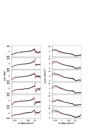
Figure 8: Comparison between fitted $S\hbox{-wave}$ amplitudes (solid circles with error bars representing statistical uncertainties) and generated amplitudes, represented as shaded regions between dashed curves computed as described in Sec. V. Generated curves follow the isobar fit model described in Sec. V. The figure shows results from the first six (of 100) samples used in the test.

The MIPWA analysis of the $S\hbox{-wave}$ component in the observed $D^{+}\rightarrow K^{-}\pi^{+}_{\scriptscriptstyle A}\pi^{+}_{\scriptscriptstyle B}$ decays relies upon a good description of the reference $P\hbox{-}$ and $D\hbox{-wave}$s.

The $P\hbox{-wave}$ defined in Eq. (10) is a combination of two Breit-Wigner’s (the $K_{1}^{*}(1410)$ is neglected), with a complex coupling coefficient (two parameters). The peak regions, $0.50<s<0.9$ ($\hbox{GeV}/c^{2}$)² and $s>2.2$  ($\hbox{GeV}/c^{2}$)², are well described by this parametrization, since data in these regions are likely to be dominated by these resonances. In the tail regions, the Breit-Wigner may be a less appropriate description of the data, since other $P\hbox{-wave}$ contributions, from non-resonant (or $I={3\over 2}$) sources, for example, could become more significant.

Two regions in the $P\hbox{-wave}$ where the tails of the BW’s dominate are $s<0.50$ ($\hbox{GeV}/c^{2}$)² and $0.9<s<2.2$ ($\hbox{GeV}/c^{2}$)². In each of these ranges the $P\hbox{-wave}$ is constructed from a linear combination of two small, complex numbers, one from each of the two BW tails. Both the phase and magnitude of the resultant are particularly sensitive to variations in the complex coupling parameters, and may not represent the $P\hbox{-wave}$ well.

The $D\hbox{-wave}$ is defined in Eq. (11), for this analysis, as a single, $L=2$ BW function. Non-resonant contributions are not expected to be significant, and interference from tails of a second resonance are absent. Eq. (11), therefore, provides a relatively good description of the $D\hbox{-wave}$.

Eqs. (2) and (3) show that the amplitude for the decays examined in this paper is a sum of six terms. Let these be labelled ${\cal S}_{\scriptscriptstyle A}$, ${\cal P}_{\scriptscriptstyle A}$ and ${\cal D}_{\scriptscriptstyle A}$ (the $S\hbox{-}$, $P\hbox{-}$ and $D\hbox{-wave}$, respectively, in the $s_{\scriptscriptstyle A}$ channel) and ${\cal S}_{\scriptscriptstyle B}$, ${\cal P}_{\scriptscriptstyle B}$ and ${\cal D}_{\scriptscriptstyle B}$ (these waves in the $s_{\scriptscriptstyle B}$ channel). The MIPWA process extracts magnitude and phase information about the $S\hbox{-wave}$ ${\cal S}_{\scriptscriptstyle A}$ from its observed interference with the complex sum of the other five amplitudes.

$${\cal T}_{\scriptscriptstyle A}={\cal P}_{\scriptscriptstyle A}+{\cal D}_{\scriptscriptstyle A}+{\cal S}_{\scriptscriptstyle B}+{\cal P}_{\scriptscriptstyle B}+{\cal D}_{\scriptscriptstyle B}.$$ (29)

The results expected from measurement of ${\cal S}_{\scriptscriptstyle A}$ can, therefore, be characterized by the dominant terms in ${\cal T}_{\scriptscriptstyle A}$ with which it interferes, and these depend on location on the Dalitz plot in Fig. 1.

As an illustration, consider measurement of ${\cal S}_{\scriptscriptstyle A}$ in the range $1.1<s<2.9$ ($\hbox{GeV}/c^{2}$)². Here, ${\cal T}_{\scriptscriptstyle A}$ is dominated by the $K^{*}(892)$ resonance band in ${\cal P}_{\scriptscriptstyle B}$ (the cross-channel). Good measurements are, therefore, expected in this range.

Next, consider the $K^{*}(892)$ peak region $1.5<s<0.9$ ($\hbox{GeV}/c^{2}$)². This region has ${\cal T}_{\scriptscriptstyle A}$ dominated by the $K^{*}(892)$ peak in ${\cal P}_{\scriptscriptstyle A}$ (the direct-channel). So good measurements are expected here too. A similar conclusion can be drawn for the $K_{1}^{*}(1680)$ peak region $s>2.9$ ($\hbox{GeV}/c^{2}$)².

Relatively poor measurements are expected for the other regions since, in these, ${\cal T}_{\scriptscriptstyle A}$ is not dominated by any one source, and is defined by a linear combination of several Breit-Wigner tails. So ${\cal T}_{\scriptscriptstyle A}$ in these regions has phase and magnitude that are sensitive to the complex couplings of $K_{1}^{*}(1680)$ and $K_{2}^{*}(1430)$ resonances.

These observations are supported by the results of the MIPWA fit shown in Fig. 3(a) and (b). It is seen that uncertainties are small for $1.1<s<2.9$ ($\hbox{GeV}/c^{2}$)² and large for $s<0.9$ ($\hbox{GeV}/c^{2}$)², improving towards the high end. In the intermediate region, $0.9<s<1.1$ ($\hbox{GeV}/c^{2}$)², the $S\hbox{-wave}$ magnitudes and phases determined in the fit exhibit significant deviations from the general trends of the neighboring points.

A.2 MC Studies with Isobar Fit

The $K_{1}^{*}(1680)$ and $K_{2}^{*}(1430)$ resonances represent small contributions to the Dalitz plot, and statistical uncertainties in their complex couplings are large enough to affect the $P\hbox{-wave}$ phase, especially in the region between $K^{*}(892)$ and $K_{1}^{*}(1680)$, as discussed in Sec. A.1. This can lead to systematic uncertainties in the $S\hbox{-wave}$ amplitudes measured. MC studies are required to estimate such effects.

MC samples of the approximate size of the data presented in this paper are generated as described by the PDF given in Eq. (17). Parameters from Table 2 for the isobar fit described in Sec. V are used for this purpose. Background events whose distributions are given in Eq. (16) are also generated to match those thought to be present in the data. Events are selected according to the efficiency $\epsilon(s_{\scriptscriptstyle A},s_{\scriptscriptstyle B})$ across the Dalitz plot.

Each sample is subjected to the MIPWA fit described in Sec. IV. In Fig. 8, $S\hbox{-wave}$ amplitudes determined in the MIPWA for the first six of the 100 samples studied are compared with those used to generate the events. The amplitudes generated come from the isobar fit, and are shown, as usual, as shaded regions between dashed curves. Phases are shown on the right and magnitudes on the left. Plots similar to Fig. 3 appear often.

The $S\hbox{-wave}$ amplitudes ($c_{k}e^{i\gamma_{k}}$) obtained are compared with those generated and, for each $k$ the normalized residuals are used to determine systematic uncertainties discussed in Sec. VII.

A.3 Other Solutions

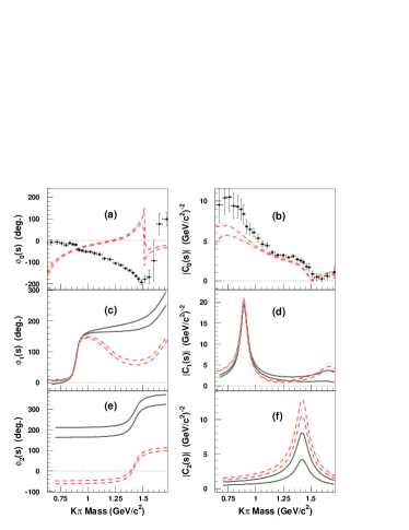
Figure 9: A second solution for the $S\hbox{-wave}$ amplitude from MIPWA fits to $D^{+}\rightarrow K^{-}\pi^{+}\pi^{+}$ decays with $P\hbox{-}$ and $D\hbox{-wave}$ parametrized by the $\kappa$ model described in the text. Plots show the (a) phase and (b) magnitude for solution B for the $S\hbox{-wave}$ obtained by using different starting values for the amplitudes. The dashed curves delineate the regions that lie within one standard deviation of the isobar model fit described in Sec. V. The $P\hbox{-wave}$ is shown in (c) and (d) and the $D\hbox{-wave}$ in (e) and (f).

The fitting procedure allows a great deal of freedom to the $S\hbox{-wave}$ amplitude. Consequently, ambiguities in solutions are anticipated. To study possible ambiguities in the MIPWA solution, fits with random starting values for the $c_{i},\gamma_{i}$ parameters, and also with different $K^{-}\pi^{+}$ mass slices are made. One other local maximum in the likelihood is found, and this is labelled solution B. The solution described in Sec. IV, and shown in Figs. 3(a) through (f), is labelled, for contrast, solution A. Solution A is the only one with an acceptable $\chi^{2}/\hbox{\small NDF}$ and has the greatest likelihood value. So it is emphasized that solutions A is, in fact, unique.

Solution B is shown in Fig. 9. It provides a qualitatively reasonable description of the distribution of the data on the Dalitz plot. However, this solution clearly exhibits retrograde motion around the unitarity circle as $K^{-}\pi^{+}$ invariant mass increases. This violates the Wigner causality principle Wigner (1955), thus eliminating it from further consideration.

The possible existence of other maxima in the likelihood, when all $S\hbox{-wave}$ magnitudes and phases are free parameters, cannot be completely ruled out. However, the solution in Sec. IV is unique in that it is the only one giving an acceptable fit probability.

References

- (1) Charge conjugate states are always implied unless explicitly stated otherwise.
- Frabetti et al. (1994) P. L. Frabetti et al. (E687), Phys. Lett. B331, 217 (1994).
- Anjos et al. (1993) J. C. Anjos et al. (E691), Phys. Rev. D48, 56 (1993).
- Frabetti et al. (1997) P. L. Frabetti et al. (E687), Phys. Lett. B407, 79 (1997).
- Aitala et al. (2001) E. M. Aitala et al. (E791), Phys. Rev. Lett. 86, 770 (2001), eprint hep-ex/0007028.
- Aitala et al. (2002) E. M. Aitala et al. (E791), Phys. Rev. Lett. 89, 121801 (2002), eprint hep-ex/0204018.
- Link et al. (2004) J. M. Link et al. (FOCUS), Phys. Lett. B585, 200 (2004), eprint hep-ex/0312040.
- Aubert et al. (2005a) B. Aubert et al. (BABAR) (2005a), Submitted to Phys. Rev. Lett.., eprint hep-ex/0504039.
- Poluektov et al. (2004) A. Poluektov et al. (Belle), Phys. Rev. D70, 072003 (2004), eprint hep-ex/0406067.
- Abe et al. (2005) K. Abe et al. (Belle) (2005), Contributed to 40th Rencontres de Moriond on Electroweak Interactions and Unified Theories, La Thuile, Aosta Valley, Italy, 5-12 Mar 2005., eprint hep-ex/0504013.
- Ablikim et al. (2004) M. Ablikim et al. (BES), Phys. Lett. B598, 149 (2004), eprint hep-ex/0406038.
- Komada (2004) T. Komada, AIP Conf. Proc. 717, 337 (2004).
- Gardner and Meissner (2002) S. Gardner and U.-G. Meissner, Phys. Rev. D65, 094004 (2002), eprint hep-ph/0112281.
- Oller (2005) J. A. Oller, Phys. Rev. D71, 054030 (2005), eprint hep-ph/0411105.
- Oller and Oset (1997) J. A. Oller and E. Oset, Nucl. Phys. A620, 438 (1997), eprint hep-ph/9702314.
- Jamin et al. (2000) M. Jamin, J. A. Oller, and A. Pich, Nucl. Phys. B587, 331 (2000), eprint hep-ph/0006045.
- Bediaga and de Miranda (2004) I. Bediaga and J. M. de Miranda (2004), Submitted to Phys. Lett. B., eprint hep-ex/0405019.
- Bediaga and de Miranda (2002) I. Bediaga and J. M. de Miranda, Phys. Lett. B550, 135 (2002), eprint hep-ph/0211078.
- Aston et al. (1988) D. Aston et al. (LASS), Nucl. Phys. B296, 493 (1988).
- Bingham et al. (1972) H. H. Bingham et al., Nucl. Phys. B41, 1 (1972).
- Estabrooks et al. (1978) P. Estabrooks et al., Nucl. Phys. B133, 490 (1978).
- Aubert et al. (2005b) B. Aubert et al. (BABAR), Phys. Rev. D71, 032005 (2005b), eprint hep-ex/0411016.
- Link et al. (2002) J. M. Link et al. (FOCUS), Phys. Lett. B535, 43 (2002), eprint hep-ex/0203031.
- Watson (1952) K. M. Watson, Phys. Rev. 88, 1163 (1952).
- Aitala et al. (1999) E. M. Aitala et al. (E791), Eur. Phys. J. direct C1, 4 (1999), eprint [http://arXiv.org/abs]hep-ex/9809029.
- (26) This definition of helicity angle differs from that used in scattering where the angle is defined as that btween and the momentum of the system.
- Hoogland et al. (1977) W. Hoogland et al., Nucl. Phys. B126, 109 (1977).
- Blatt and Weisskopf (1952) J. M. Blatt and V. F. Weisskopf, Wiley, New York p. 361 (1952).
- Tornqvist (1995) N. A. Tornqvist, Z. Phys. C68, 647 (1995), eprint hep-ph/9504372.
- (30) It has often been suggested that the denominator should include a factor where is the location of the Adler zero required in scattering.
- (31) To avoid difficulties arising from the periodic nature of the phase , the interpolation is made in the values of the real and imaginary parts of the amplitude . For each of these, quadratic functions are defined to the left and right of each such that their first derivatives are equal at each point.
- S. Eidelman et al. (2004) S. Eidelman et al. (PDG), Physics Letters B 592, 1 (2004), URL http://pdg.lbl.gov.
- (33) Other local minima are also found. These are discussed in Appendix A. The fit solutions described here give the greatest likelihood value and, based on , the best description of the data.
- Bugg (2005) D. V. Bugg (2005), eprint hep-ex/0510019.
- Edera and Pennington (2005) L. Edera and M. R. Pennington (2005), have recently elaborated on this point., eprint hep-ph/0506117.
- Wigner (1955) E. P. Wigner, Phys. Rev. 98, 145 (1955).