SNO Collaboration

A Search for Periodicities in the ⁸B Solar Neutrino Flux
Measured by the Sudbury Neutrino Observatory

B. Aharmim Department of Physics and Astronomy, Laurentian University, Sudbury, Ontario P3E 2C6, Canada S.N. Ahmed Department of Physics, Queen’s University, Kingston, Ontario K7L 3N6, Canada A.E. Anthony Department of Physics, University of Texas at Austin, Austin, TX 78712-0264 E.W. Beier Department of Physics and Astronomy, University of Pennsylvania, Philadelphia, PA 19104-6396 A. Bellerive Ottawa-Carleton Institute for Physics, Department of Physics, Carleton University, Ottawa, Ontario K1S 5B6, Canada M. Bergevin Physics Department, University of Guelph, Guelph, Ontario N1G 2W1, Canada S.D. Biller Department of Physics, University of Oxford, Denys Wilkinson Building, Keble Road, Oxford OX1 3RH, UK M.G. Boulay Los Alamos National Laboratory, Los Alamos, NM 87545 M.G. Bowler Department of Physics, University of Oxford, Denys Wilkinson Building, Keble Road, Oxford OX1 3RH, UK Y.D. Chan Institute for Nuclear and Particle Astrophysics and Nuclear Science Division, Lawrence Berkeley National Laboratory, Berkeley, CA 94720 M. Chen Department of Physics, Queen’s University, Kingston, Ontario K7L 3N6, Canada X. Chen Present address: Stanford Linear Accelerator Center, Menlo Park, CA Institute for Nuclear and Particle Astrophysics and Nuclear Science Division, Lawrence Berkeley National Laboratory, Berkeley, CA 94720 B.T. Cleveland Department of Physics, University of Oxford, Denys Wilkinson Building, Keble Road, Oxford OX1 3RH, UK T. Costin Department of Physics and Astronomy, University of British Columbia, Vancouver, BC V6T 1Z1, Canada G.A. Cox Center for Experimental Nuclear Physics and Astrophysics, and Department of Physics, University of Washington, Seattle, WA 98195 C.A. Currat Institute for Nuclear and Particle Astrophysics and Nuclear Science Division, Lawrence Berkeley National Laboratory, Berkeley, CA 94720 X. Dai Ottawa-Carleton Institute for Physics, Department of Physics, Carleton University, Ottawa, Ontario K1S 5B6, Canada H. Deng Department of Physics and Astronomy, University of Pennsylvania, Philadelphia, PA 19104-6396 J. Detwiler Center for Experimental Nuclear Physics and Astrophysics, and Department of Physics, University of Washington, Seattle, WA 98195 P.J. Doe Center for Experimental Nuclear Physics and Astrophysics, and Department of Physics, University of Washington, Seattle, WA 98195 R.S. Dosanjh Ottawa-Carleton Institute for Physics, Department of Physics, Carleton University, Ottawa, Ontario K1S 5B6, Canada G. Doucas Department of Physics, University of Oxford, Denys Wilkinson Building, Keble Road, Oxford OX1 3RH, UK C.A. Duba Center for Experimental Nuclear Physics and Astrophysics, and Department of Physics, University of Washington, Seattle, WA 98195 F.A. Duncan Department of Physics, Queen’s University, Kingston, Ontario K7L 3N6, Canada M. Dunford Department of Physics and Astronomy, University of Pennsylvania, Philadelphia, PA 19104-6396 J.A. Dunmore Present address: Department of Physics, University of California, Irvine, CA Department of Physics, University of Oxford, Denys Wilkinson Building, Keble Road, Oxford OX1 3RH, UK E.D. Earle Department of Physics, Queen’s University, Kingston, Ontario K7L 3N6, Canada S.R. Elliott Los Alamos National Laboratory, Los Alamos, NM 87545 H.C. Evans Department of Physics, Queen’s University, Kingston, Ontario K7L 3N6, Canada G.T. Ewan Department of Physics, Queen’s University, Kingston, Ontario K7L 3N6, Canada J. Farine Department of Physics and Astronomy, Laurentian University, Sudbury, Ontario P3E 2C6, Canada H. Fergani Department of Physics, University of Oxford, Denys Wilkinson Building, Keble Road, Oxford OX1 3RH, UK F. Fleurot Department of Physics and Astronomy, Laurentian University, Sudbury, Ontario P3E 2C6, Canada J.A. Formaggio Center for Experimental Nuclear Physics and Astrophysics, and Department of Physics, University of Washington, Seattle, WA 98195 W. Frati Department of Physics and Astronomy, University of Pennsylvania, Philadelphia, PA 19104-6396 B.G. Fulsom Department of Physics, Queen’s University, Kingston, Ontario K7L 3N6, Canada N. Gagnon Center for Experimental Nuclear Physics and Astrophysics, and Department of Physics, University of Washington, Seattle, WA 98195 J.TM. Goon Department of Physics and Astronomy, Louisiana State University, Baton Rouge, LA 70803 K. Graham Department of Physics, Queen’s University, Kingston, Ontario K7L 3N6, Canada R.L. Hahn Chemistry Department, Brookhaven National Laboratory, Upton, NY 11973-5000 A.L. Hallin Department of Physics, Queen’s University, Kingston, Ontario K7L 3N6, Canada E.D. Hallman Department of Physics and Astronomy, Laurentian University, Sudbury, Ontario P3E 2C6, Canada W.B. Handler Department of Physics, Queen’s University, Kingston, Ontario K7L 3N6, Canada C.K. Hargrove Ottawa-Carleton Institute for Physics, Department of Physics, Carleton University, Ottawa, Ontario K1S 5B6, Canada P.J. Harvey Department of Physics, Queen’s University, Kingston, Ontario K7L 3N6, Canada R. Hazama Present address: Department of Physics, Osaka University, Osaka, Japan Center for Experimental Nuclear Physics and Astrophysics, and Department of Physics, University of Washington, Seattle, WA 98195 K.M. Heeger Institute for Nuclear and Particle Astrophysics and Nuclear Science Division, Lawrence Berkeley National Laboratory, Berkeley, CA 94720 L. Heelan Ottawa-Carleton Institute for Physics, Department of Physics, Carleton University, Ottawa, Ontario K1S 5B6, Canada W.J. Heintzelman Department of Physics and Astronomy, University of Pennsylvania, Philadelphia, PA 19104-6396 J. Heise Los Alamos National Laboratory, Los Alamos, NM 87545 R.L. Helmer TRIUMF, 4004 Wesbrook Mall, Vancouver, BC V6T 2A3, Canada R.J. Hemingway Ottawa-Carleton Institute for Physics, Department of Physics, Carleton University, Ottawa, Ontario K1S 5B6, Canada A. Hime Los Alamos National Laboratory, Los Alamos, NM 87545 M.A. Howe Center for Experimental Nuclear Physics and Astrophysics, and Department of Physics, University of Washington, Seattle, WA 98195 M. Huang Department of Physics, University of Texas at Austin, Austin, TX 78712-0264 E. Inrig Ottawa-Carleton Institute for Physics, Department of Physics, Carleton University, Ottawa, Ontario K1S 5B6, Canada P. Jagam Physics Department, University of Guelph, Guelph, Ontario N1G 2W1, Canada N.A. Jelley Department of Physics, University of Oxford, Denys Wilkinson Building, Keble Road, Oxford OX1 3RH, UK J.R. Klein Department of Physics, University of Texas at Austin, Austin, TX 78712-0264 L.L. Kormos Department of Physics, Queen’s University, Kingston, Ontario K7L 3N6, Canada M.S. Kos Los Alamos National Laboratory, Los Alamos, NM 87545 A. Krüger Department of Physics and Astronomy, Laurentian University, Sudbury, Ontario P3E 2C6, Canada C. Kraus Department of Physics, Queen’s University, Kingston, Ontario K7L 3N6, Canada C.B. Krauss Department of Physics, Queen’s University, Kingston, Ontario K7L 3N6, Canada A.V. Krumins Department of Physics, Queen’s University, Kingston, Ontario K7L 3N6, Canada T. Kutter Department of Physics and Astronomy, Louisiana State University, Baton Rouge, LA 70803 C.C.M. Kyba Department of Physics and Astronomy, University of Pennsylvania, Philadelphia, PA 19104-6396 H. Labranche Physics Department, University of Guelph, Guelph, Ontario N1G 2W1, Canada R. Lange Chemistry Department, Brookhaven National Laboratory, Upton, NY 11973-5000 J. Law Physics Department, University of Guelph, Guelph, Ontario N1G 2W1, Canada I.T. Lawson Present address: SNOLAB, INCO Creighton #9 Mine, P.O. Box 159, Lively, Ontario P3Y 1M3, Canada Physics Department, University of Guelph, Guelph, Ontario N1G 2W1, Canada K.T. Lesko Institute for Nuclear and Particle Astrophysics and Nuclear Science Division, Lawrence Berkeley National Laboratory, Berkeley, CA 94720 J.R. Leslie Department of Physics, Queen’s University, Kingston, Ontario K7L 3N6, Canada I. Levine Present Address: Department of Physics and Astronomy, Indiana University, South Bend, IN Ottawa-Carleton Institute for Physics, Department of Physics, Carleton University, Ottawa, Ontario K1S 5B6, Canada J.C. Loach Department of Physics, University of Oxford, Denys Wilkinson Building, Keble Road, Oxford OX1 3RH, UK S. Luoma Department of Physics and Astronomy, Laurentian University, Sudbury, Ontario P3E 2C6, Canada R. MacLellan Department of Physics, Queen’s University, Kingston, Ontario K7L 3N6, Canada S. Majerus Department of Physics, University of Oxford, Denys Wilkinson Building, Keble Road, Oxford OX1 3RH, UK J. Maneira Laboratório de Instrumentação e Física Experimental de Partículas, Av. Elias Garcia 14, 1^∘, 1000-149 Lisboa, Portugal A.D. Marino Present address: Fermilab, Batavia, IL Institute for Nuclear and Particle Astrophysics and Nuclear Science Division, Lawrence Berkeley National Laboratory, Berkeley, CA 94720 N. McCauley Department of Physics and Astronomy, University of Pennsylvania, Philadelphia, PA 19104-6396 A.B. McDonald Department of Physics, Queen’s University, Kingston, Ontario K7L 3N6, Canada S. McGee Center for Experimental Nuclear Physics and Astrophysics, and Department of Physics, University of Washington, Seattle, WA 98195 C. Mifflin Ottawa-Carleton Institute for Physics, Department of Physics, Carleton University, Ottawa, Ontario K1S 5B6, Canada K.K.S. Miknaitis Center for Experimental Nuclear Physics and Astrophysics, and Department of Physics, University of Washington, Seattle, WA 98195 B.G. Nickel Physics Department, University of Guelph, Guelph, Ontario N1G 2W1, Canada A.J. Noble Department of Physics, Queen’s University, Kingston, Ontario K7L 3N6, Canada E.B. Norman Present address: Lawrence Livermore National Laboratory, Livermore, CA Institute for Nuclear and Particle Astrophysics and Nuclear Science Division, Lawrence Berkeley National Laboratory, Berkeley, CA 94720 N.S. Oblath Center for Experimental Nuclear Physics and Astrophysics, and Department of Physics, University of Washington, Seattle, WA 98195 C.E. Okada Institute for Nuclear and Particle Astrophysics and Nuclear Science Division, Lawrence Berkeley National Laboratory, Berkeley, CA 94720 H.M. O’Keeffe Department of Physics, University of Oxford, Denys Wilkinson Building, Keble Road, Oxford OX1 3RH, UK R.W. Ollerhead Physics Department, University of Guelph, Guelph, Ontario N1G 2W1, Canada G.D. Orebi Gann Department of Physics, University of Oxford, Denys Wilkinson Building, Keble Road, Oxford OX1 3RH, UK J.L. Orrell Present address: Pacific Northwest National Laboratory, Richland, WA Center for Experimental Nuclear Physics and Astrophysics, and Department of Physics, University of Washington, Seattle, WA 98195 S.M. Oser Department of Physics and Astronomy, University of British Columbia, Vancouver, BC V6T 1Z1, Canada T. Ouvarova Ottawa-Carleton Institute for Physics, Department of Physics, Carleton University, Ottawa, Ontario K1S 5B6, Canada S.J.M. Peeters Department of Physics, University of Oxford, Denys Wilkinson Building, Keble Road, Oxford OX1 3RH, UK A.W.P. Poon Institute for Nuclear and Particle Astrophysics and Nuclear Science Division, Lawrence Berkeley National Laboratory, Berkeley, CA 94720 C.S.J. Pun Present address: Department of Physics, The University of Hong Kong, Hong Kong. Institute for Nuclear and Particle Astrophysics and Nuclear Science Division, Lawrence Berkeley National Laboratory, Berkeley, CA 94720 K. Rielage Center for Experimental Nuclear Physics and Astrophysics, and Department of Physics, University of Washington, Seattle, WA 98195 B.C. Robertson Department of Physics, Queen’s University, Kingston, Ontario K7L 3N6, Canada R.G.H. Robertson Center for Experimental Nuclear Physics and Astrophysics, and Department of Physics, University of Washington, Seattle, WA 98195 E. Rollin Ottawa-Carleton Institute for Physics, Department of Physics, Carleton University, Ottawa, Ontario K1S 5B6, Canada S.S.E. Rosendahl Present address: Lund University, Sweden Institute for Nuclear and Particle Astrophysics and Nuclear Science Division, Lawrence Berkeley National Laboratory, Berkeley, CA 94720 M.H. Schwendener Department of Physics and Astronomy, Laurentian University, Sudbury, Ontario P3E 2C6, Canada S.R. Seibert Department of Physics, University of Texas at Austin, Austin, TX 78712-0264 O. Simard Ottawa-Carleton Institute for Physics, Department of Physics, Carleton University, Ottawa, Ontario K1S 5B6, Canada J.J. Simpson Physics Department, University of Guelph, Guelph, Ontario N1G 2W1, Canada C.J. Sims Department of Physics, University of Oxford, Denys Wilkinson Building, Keble Road, Oxford OX1 3RH, UK D. Sinclair Ottawa-Carleton Institute for Physics, Department of Physics, Carleton University, Ottawa, Ontario K1S 5B6, Canada L. Sinclair Ottawa-Carleton Institute for Physics, Department of Physics, Carleton University, Ottawa, Ontario K1S 5B6, Canada P. Skensved Department of Physics, Queen’s University, Kingston, Ontario K7L 3N6, Canada M.W.E. Smith Center for Experimental Nuclear Physics and Astrophysics, and Department of Physics, University of Washington, Seattle, WA 98195 R.G. Stokstad Institute for Nuclear and Particle Astrophysics and Nuclear Science Division, Lawrence Berkeley National Laboratory, Berkeley, CA 94720 L.C. Stonehill Center for Experimental Nuclear Physics and Astrophysics, and Department of Physics, University of Washington, Seattle, WA 98195 R. Tafirout Present Address: TRIUMF, 4004 Wesbrook Mall, Vancouver, BC V6T 2A3, Canada Department of Physics and Astronomy, Laurentian University, Sudbury, Ontario P3E 2C6, Canada Y. Takeuchi Department of Physics, Queen’s University, Kingston, Ontario K7L 3N6, Canada G. Tešić Ottawa-Carleton Institute for Physics, Department of Physics, Carleton University, Ottawa, Ontario K1S 5B6, Canada M. Thomson Department of Physics, Queen’s University, Kingston, Ontario K7L 3N6, Canada K.V. Tsang Present address: Department of Physics, The University of Hong Kong, Hong Kong. Institute for Nuclear and Particle Astrophysics and Nuclear Science Division, Lawrence Berkeley National Laboratory, Berkeley, CA 94720 T. Tsui Department of Physics and Astronomy, University of British Columbia, Vancouver, BC V6T 1Z1, Canada R. Van Berg Department of Physics and Astronomy, University of Pennsylvania, Philadelphia, PA 19104-6396 C.J. Virtue Department of Physics and Astronomy, Laurentian University, Sudbury, Ontario P3E 2C6, Canada B.L. Wall Center for Experimental Nuclear Physics and Astrophysics, and Department of Physics, University of Washington, Seattle, WA 98195 D. Waller Ottawa-Carleton Institute for Physics, Department of Physics, Carleton University, Ottawa, Ontario K1S 5B6, Canada C.E. Waltham Department of Physics and Astronomy, University of British Columbia, Vancouver, BC V6T 1Z1, Canada H. Wan Chan Tseung Department of Physics, University of Oxford, Denys Wilkinson Building, Keble Road, Oxford OX1 3RH, UK D.L. Wark Additional Address: Imperial College, London SW7 2AZ, UK Rutherford Appleton Laboratory, Chilton, Didcot OX11 0QX, UK J. Wendland Department of Physics and Astronomy, University of British Columbia, Vancouver, BC V6T 1Z1, Canada N. West Department of Physics, University of Oxford, Denys Wilkinson Building, Keble Road, Oxford OX1 3RH, UK J.F. Wilkerson Center for Experimental Nuclear Physics and Astrophysics, and Department of Physics, University of Washington, Seattle, WA 98195 J.R. Wilson Present address: Department of Physics and Astronomy, University of Sussex, Brighton BN1 9QH, UK Department of Physics, University of Oxford, Denys Wilkinson Building, Keble Road, Oxford OX1 3RH, UK J.M. Wouters Los Alamos National Laboratory, Los Alamos, NM 87545 M. Yeh Chemistry Department, Brookhaven National Laboratory, Upton, NY 11973-5000 K. Zuber Present address: Department of Physics and Astronomy, University of Sussex, Brighton BN1 9QH, UK Department of Physics, University of Oxford, Denys Wilkinson Building, Keble Road, Oxford OX1 3RH, UK

(July 18, 2005; Revised August 4, 2005; to appear as Phys Rev D 72, 052010)

Abstract

A search has been made for sinusoidal periodic variations in the ⁸B solar neutrino flux using data collected by the Sudbury Neutrino Observatory over a 4-year time interval. The variation at a period of one year is consistent with modulation of the ⁸B neutrino flux by the Earth’s orbital eccentricity. No significant sinusoidal periodicities are found with periods between 1 day and 10 years with either an unbinned maximum likelihood analysis or a Lomb-Scargle periodogram analysis. The data are inconsistent with the hypothesis that the results of the recent analysis by Sturrock et al., based on elastic scattering events in Super-Kamiokande, can be attributed to a 7% sinusoidal modulation of the total ⁸B neutrino flux.

pacs:

26.65+t, 95.75.Wx, 14.60.St, 96.60.Vg

I Introduction

There have been recent reports of periodic variations in the measured solar neutrino fluxes sturrock_sk1 ; sturrock_sk2 ; sturrock_sk3 ; sturrock_gallex1 ; sturrock_gallex2 ; sturrock_gallex3 ; milsztajn ; ranucci . Other analyses of these same data, including analyses by the experimental collaborations themselves, have failed to find such evidence sk ; pandola . The reported periods have been claimed to be related to the solar rotational period. Particularly relevant for this paper is a claimed 7% amplitude modulation in Super-Kamiokande’s ⁸B neutrino flux at a frequency of 9.43 y^-1 sturrock_sk2 ; sturrock_sk3 . Because solar rotation should not produce variations in the solar nuclear fusion rate, non-standard neutrino properties have been proposed as an explanation. For example, the coupling of a neutrino magnetic moment to rotating magnetic fields inside the Sun might cause solar neutrinos to transform into other flavors through a resonant spin flavor precession mechanism rsfp1 ; rsfp2 ; rsfp3 . Periodicities in the solar neutrino flux, if confirmed, could provide evidence for new neutrino physics beyond the commonly accepted picture of matter-enhanced oscillation of massive neutrinos.

This paper presents a search for periodicities in the data from the Sudbury Neutrino Observatory (SNO). SNO is a real-time, water Cherenkov detector located in the Inco, Ltd. Creighton nickel mine near Sudbury, Ontario, Canada sno_nim . SNO observes charged-current (CC) and neutral-current (NC) interactions of ⁸B neutrinos on deuterons in 1 ktonne of D₂O, as well as neutrino-electron elastic scattering (ES) interactions. By comparing the observed rates of CC, NC, and ES interactions, SNO has demonstrated that a substantial fraction of ⁸B electron neutrinos produced inside the Sun transform into other active neutrino flavors cc_prl ; d2o_prl ; dn_prl ; salt_prl ; nsp .

SNO’s combination of real-time detection, low backgrounds, and sensitivity to different neutrino flavors give it unique capabilities in a search for neutrino flux periodicities. Chief among these is the ability to do an unbinned analysis, in which the event times of individual neutrino events are used as inputs to a maximum likelihood fit.

This paper presents results from an unbinned maximum likelihood analysis and a more traditional Lomb-Scargle periodogram analysis for SNO’s pure D₂O and salt phase data sets. Previous analyses of data from other experiments have used the Lomb-Scargle periodogram scargle and binned maximum likelihood techniques to search for periodicities in the solar neutrino data. These data generally consist of flux values measured in a number of time bins of unequal size. Because analyses of binned data can be sensitive to the choice of binning, which can also produce aliasing effects, it is desirable to avoid binning the data if possible. Section II describes the data sets. Section III contains the results of a general search for any periodicities with periods between 1 day and 10 years. Section IV presents limits on the amplitudes at two specific frequencies: the 9.43 y^-1 modulation of the ⁸B neutrino flux claimed by Sturrock et al. sturrock_sk2 ; sturrock_sk3 , and a yearly modulation due to the Earth’s orbital eccentricity.

II Description of the SNO data sets

The data included in these analyses consist of the selected neutrino events for the initial phase of SNO, in which the detector contained pure D₂O d2o_prl , and for SNO’s salt phase, in which 2 tonnes of NaCl were added to the D₂O to increase the neutron detection efficiency for the NC reaction nsp . Each data set is divided into runs of varying length during which the detector was live for solar neutrino events. The D₂O data set consists of 559 runs starting on November 2, 1999, and spans a calendar period of 572.2 days during which the total neutrino livetime was 312.9 days. The salt phase of SNO started on July 26, 2001, 59.7 calendar days after the end of the pure D₂O phase of the experiment. The salt data set contains 1212 runs and spans a calendar period of 762.7 days during which the total neutrino livetime was 398.6 days. The intervals between runs during which SNO was not recording solar neutrino events correspond to run transitions, detector maintenance, calibration activities, periods when the detector was off, etc. Deadtime incurred within a run, mostly due to spallation cuts that remove events occurring within 20 seconds after a muon, can be neglected, since such deadtime is incurred randomly at average intervals much shorter than the periods of interest for this analysis. This deadtime is 2.1% for the D₂O data set and 1.8% for the salt data set.

The event selection for the data sets is similar to that in d2o_prl and nsp . Events were selected inside a reconstructed fiducial volume of $R<550$ cm and above an effective kinetic energy of $T_{\text{eff}}>5$ MeV (D₂O) or $T_{\text{eff}}>5.5$ MeV (salt). The salt data set contains 4722 events, as in nsp . During the salt analysis described in nsp a background of “event bursts”, consisting of two or three neutron-like events occurring in a short time interval, was identified and removed with a cut that eliminated any event occurring within 50 ms of an otherwise acceptable candidate neutrino event. The source of these 11 bursts is not certain, but they may have been produced by atmospheric neutrino interactions. For this analysis a similar cut removing any event occurring within 150 ms of another event was applied to the D₂O data, reducing the number of selected events from 2928, as in d2o_prl , to 2924. The timing window for the cut in the D₂O data is longer than for the salt data to account for the longer neutron capture time in pure D₂O.

An important element of a periodicity analysis is exact knowledge of when each data-taking run began and ended. These run boundaries define the time exposure of the data set, which itself may induce frequency components that could impact a periodicity analysis. The unbinned maximum likelihood analysis described below makes explicit use of these run boundary times, and all Monte Carlo simulations are generated using the exact run boundaries, even if the simulated data are binned in a following analysis. These precautions avoid ad hoc assumptions about the distribution of the time exposure within any time bin. The measured time for each event was measured with a global positioning system (GPS) clock to a precision of $\sim 100$ ns, but rounded to 10 ms accuracy for the analysis. The run boundary times were determined from the times of the first and last events in each run with a precision of $\sim 50$ ms.

Refer to caption — Figure 1: The livetime-corrected 1-day total rate of events as a function of time for the D₂O and salt phases. The weighted mean rates are $9.35\pm 0.17$ and $11.85\pm 0.17$ events/day, respectively.

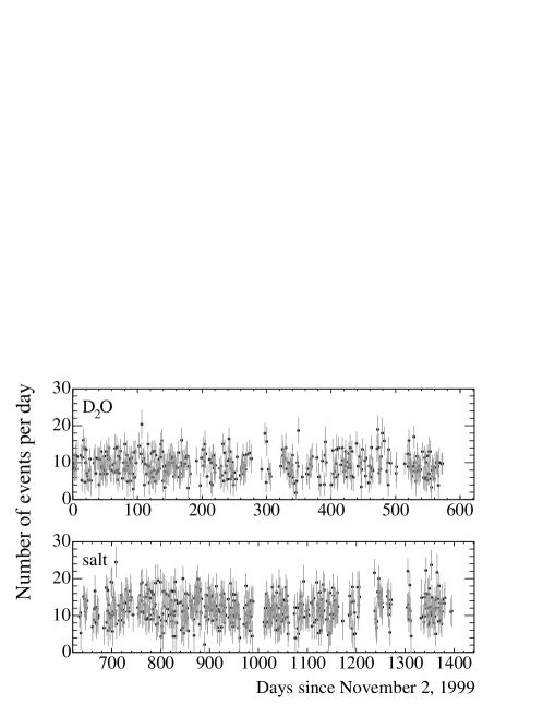
Figure 1 displays the solar neutrino event rate in livetime corrected 1-day bins over the total exposure time of both phases of SNO sno_data . The D₂O and salt data sets may be individually examined for periodicities, or the combined data from both phases can be jointly searched. It should be noted that the relative amounts of CC, NC, and ES events are different for the D₂O and salt data, with the salt data set containing a much higher fraction of NC events.

Although SNO’s data sets are dominated by solar neutrino events, they also contain a small number of non-neutrino backgrounds, primarily neutrons produced through photodisintegration of deuterons by internal or external radioactivity. The total estimated number of background events is 123 ${}^{+22}_{-17}$ for the D₂O data set (4.2 ${}^{+0.8}_{-0.6}$ % of the total rate), and 260 $\pm 59$ events for the salt data set (5.5 $\pm 1.2$ % of the total rate). Although the background rate is not entirely constant, the backgrounds are small and stable enough that they can be neglected in this analysis.

III General Periodicity Search

Both an unbinned maximum likelihood analysis and a Lomb-Scargle periodogram with 1-day binning were used to search SNO’s data for periodicities. Results are presented below for the D₂O, salt, and combined data from each method, along with evaluations of the sensitivity of each method to sinusoidal variations of various periods and amplitudes. The periodicity searches were carried out over the sum of CC, NC, and ES events.

Extensive use was made of Monte Carlo data sets to evaluate the statistical significance of the results and the sensitivity of each method. To determine the statistical significance of any peak in the frequency spectrum, 10,000 Monte Carlo data sets with events generated randomly within the run boundaries for each phase were used, with mean event rates in each phase matching those observed in SNO’s data sets. The number of events in each Monte Carlo data set was drawn from a Poisson distribution with the same average rate as the data, and the events were distributed uniformly within the run boundaries footnote1 . These “null-hypothesis” Monte Carlo data sets were used to determine the probability that a data set drawn from a constant rate distribution would produce a false positive detection of a periodicity. To determine the sensitivity of an analysis to a real periodicity, 1,000 Monte Carlo data sets were generated for each of several combinations of frequencies and amplitudes, with the events drawn from a time distribution of the form $1+A\cos(2\pi ft)$ . The sensitivity for any frequency $f$ and amplitude $A$ is then defined as the probability that the analysis will reject the null hypothesis of a constant rate at the 99% confidence level.

III.1 Unbinned Maximum Likelihood Method

The unbinned maximum likelihood method tests the hypothesis that the observed events are drawn from a rate distribution given by

\phi(t)=N(1+A\cos(2\pi ft+\delta))

(1)

relative to the hypothesis that they are drawn from a constant rate distribution ( $A=0$ ). $A$ is the fractional amplitude of the periodic variation about the mean, $\delta$ is a phase offset, and $N$ is a normalization constant for the rate. Equation 1 serves as the probability density function (PDF) for the observed event times, which are additionally constrained to occur only within run boundaries (i.e., $\phi(t)=0$ if $t$ is not between the start and end times of any run).

With $f$ fixed, the maximum of the extended likelihood $L(t_{k}|N,A,\delta,f)$ as a function of the individual event times $t_{k}$ is calculated for a data set as

\ln L(t_{k}|N,A,\delta,f)=-\sum_{j=1}^{\text{runs}}\int_{t_{i}^{j}}^{t_{f}^{j}}\!\phi(t)dt+\sum_{k=1}^{\text{events}}\ln(\phi(t_{k}))

(2)

where the first term is a sum over all runs of an integral evaluated between each run’s start and stop times $t_{i}^{j}$ and $t_{f}^{j}$ , and accounts for Poisson fluctuations in the signal amplitude. The second term is a sum over the events in the data set, and $t_{k}$ is the time of the $k$ th event. The log likelihood is maximized as a function of $A$ , $\delta$ , and $N$ to yield $\ln L_{\text{max}}$ , while $f$ is kept fixed. Then the constraint $A=0$ is imposed, removing the dependence of $\phi(t)$ on both $A$ and $\delta$ , and the log likelihood is maximized over the remaining free parameter $N$ to yield $\ln L_{\text{max}}(A=0)$ . By the likelihood ratio theorem likelihood the difference $2S\equiv 2(\ln L_{\text{max}}-\ln L_{\text{max}}(A=0))$ will approximately have a $\chi^{2}$ distribution with two degrees of freedom (since the choice $A=0$ also removes the dependence on the phase $\delta$ ). Thus $S$ will follow a simple exponential if the true value of $A$ is zero. Therefore, at any single frequency $f$ , the probability of observing $S>Z$ under the null hypothesis that $\phi(t)=N$ is approximately $e^{-Z}$ . This null hypothesis test is carried out for a large set of frequencies scanning the region of interest.

Equation 2 includes both a floating offset $N$ and an amplitude $A$ as free parameters. Allowing both of these parameters to vary is necessary to deal with very low frequencies, for which $N$ and $A$ become degenerate parameters. Simply fixing $N$ to the mean rate, as was done in sturrock_sk3 , will be prone to bias at the very lowest frequencies, but gives virtually identical results to the floating offset procedure when the length of the data set is longer than the period $T=1/f$ , since in this case enough cycles are sampled to break the degeneracy between $N$ and $A$ .

Equations 1 and 2 are adequate to test for periodicity in a single data set, but for a combined analysis of SNO’s D₂O and salt data sets, account must be taken of the differing mean rates owing to different detection efficiencies and energy thresholds in the two phases. This can be done by generalizing $\phi(t)$ to:

	$\displaystyle\phi(t)$	$\displaystyle=$	$\displaystyle N_{\text{d2o}}(1+A\cos(2\pi ft+\delta)),{\rm~{}if~{}}t\in{\rm~{}D}_{2}{\rm O~{}run}$
	$\displaystyle\phi(t)$	$\displaystyle=$	$\displaystyle N_{\text{salt}}(1+A\cos(2\pi ft+\delta)),{\rm~{}if~{}}t\in{\rm~{}salt~{}run}$

This PDF allows different normalization constants for the two data sets, while retaining the assumption that the flux variation has the same fractional amplitude in both the D₂O and salt data.

III.1.1 Results for the SNO data sets

Figure 2 shows $S$ as a function of frequency for the D₂O, salt, and combined data sets at 3650 frequencies with periods ranging from 10 years down to 1 day, with a sampling interval of $\Delta f=1/(3650~{}{\rm days})$ . This corresponds to an oversampling of the number of independent Fourier frequencies for continuous data by a factor of approximately 5-6 for the separate D₂O and salt data sets, and a factor of 2.6 for the combined data set. The maximum value of $S$ for the D₂O data set is $S=7.1$ at a period of 3.50 days ( $f=0.296$ days^-1). The largest peak found in the salt data has a height of $S=9.4$ at a period of 1.03 days ( $f=0.971$ days^-1), while the combined data set has its largest peak of $S=8.8$ at a period of 2.40 days ( $f=0.417$ days^-1).

Figure 3 shows the distribution of maximum peak heights for 10,000 Monte Carlo data sets generated with no periodicity and analyzed identically to SNO’s combined data set. Distributions for the D₂O and salt Monte Carlo data sets analyzed individually look similar. Of the 10,000 simulated data sets, 35% yielded at least one peak with $S>8.8$ , exceeding the largest peak seen in SNO’s combined data set. For the D₂O Monte Carlo data sets, 72% had a peak larger than the observed largest peak of $S=7.1$ , while 14% of the salt Monte Carlo data sets yielded a peak larger than the $S=9.4$ peak seen in the data. Therefore, none of the observed peaks are statistically significant.

Under the null hypothesis of no time variability, the probability of any individual frequency having $S$ smaller than some threshold $Z$ is approximately $1-e^{-Z}$ . If all 3650 scanned frequencies were statistically independent, the probability that all peaks would be smaller than $Z$ would be $(1-e^{-Z})^{3650}$ . However, the 3650 scanned frequencies are not strictly independent, since a finite data set has limited frequency resolution, and neighboring frequencies are correlated. If $F$ is the effective number of independent frequencies, then the probability distribution for the height $Z$ of the largest peak approximately follows

P(Z)~{}dZ\propto e^{-Z}(1-e^{-Z})^{F-1}~{}dZ

(3)

The effective number of independent frequencies increases with the length of the data set and number of detected events. Fitting the Monte Carlo distributions for $Z$ to this equation yields $F=1422\pm 17$ for the D₂O, $F=1696\pm 26$ for the salt, and $F=2739\pm 30$ for the combined data set. Figure 3 shows this fit for the combined analysis. These values are consistent with expectations based on the oversampling factors described in Section III.1.1 orford . Although Equation 3 appears to model $P(Z)$ well, quoted significance levels are always determined directly from the Monte Carlo distributions and not from the analytic formula. To ensure that no significant peaks were missed, the combined analysis of the actual data (but not the Monte Carlo data sets) was repeated with the sampling increased by a factor of five. No new peaks were found.

III.1.2 Sensitivity to sinusoidal periodicities

Distributions of the maximum peak height for Monte Carlo data sets, such as in Figure 3, readily yield the threshold $\zeta$ for which 99% of Monte Carlo data sets generated without periodicity would yield a maximum peak height of $\zeta$ or less. This threshold defines the peak height at which the null hypothesis of no time variation is rejected at the 99% confidence level, and equals 12.10, 12.20, and 12.65 for the D₂O, salt, and combined data sets respectively.

Monte Carlo data sets drawn from rate distributions with sinusoidal periodicities of various periods and amplitudes were analyzed to determine the probability of rejecting the null hypothesis at the 99% C.L.

Figure 4 shows the amplitudes as a function of period at which the method has a 50% (90%) probability of rejecting the null hypothesis, for simulations of SNO’s combined data set. While the sensitivity varies as a function of period, a signal must have an amplitude of approximately 8% to be discovered 50% of the time.

III.2 The Lomb-Scargle periodogram

The Lomb-Scargle periodogram is a method for searching unevenly sampled data for sinusoidal periodicities scargle and provides an alternative to the unbinned maximum likelihood technique described above.

The Lomb-Scargle power $P(f)$ at frequency $f$ is calculated from the measured flux values $y(t_{i})$ in $N$ independent time bins as:

P(f)=\frac{1}{2\sigma^{2}}\left(\frac{\left[\sum_{i=1}^{N}w_{i}(y(t_{i})-\bar{y})\cos(2\pi f(t_{i}-\tau))\right]^{2}}{\sum_{i=1}^{N}w_{i}\cos^{2}(2\pi f(t_{i}-\tau))}\\ +\frac{\left[\sum_{i=1}^{N}w_{i}(y(t_{i})-\bar{y})\sin(2\pi f(t_{i}-\tau))\right]^{2}}{\sum_{i=1}^{N}w_{i}\sin^{2}(2\pi f(t_{i}-\tau))}\right)\\

(4)

where the phase factor $\tau$ satisfies:

{\rm tan}(4\pi f\tau)=\frac{\sum_{i=1}^{N}w_{i}\sin(4\pi ft_{i})}{\sum_{i=1}^{N}w_{i}\cos(4\pi ft_{i})}

Each bin is weighted in proportion to the inverse of its squared uncertainty divided by the average value of the inverse of the squared uncertainty $\langle 1/\sigma_{i}^{2}\rangle$ (so $w_{i}=1/\sigma_{i}^{2}/\langle 1/\sigma_{i}^{2}\rangle$ ), as in sturrock_sk3 . In Equation 4 $t_{i}$ is the livetime-weighted mean time for the $i$ th bin, and $\bar{y}$ and $\sigma^{2}$ are the weighted mean and weighted variance of the data for all the bins calculated with the weighting factors $w_{i}$ .

Like the maximum likelihood method, the power $P$ in the Lomb-Scargle periodogram at any single frequency $f$ is expected to approximately follow an exponential distribution $e^{-P}$ if the data set is drawn from a constant rate distribution. The same methods of evaluating the significance of the largest peak and the sensitivity of the method to periodic signals can be employed, making use of large numbers of Monte Carlo data sets.

In sk the Super-Kamiokande collaboration used an unweighted Lomb-Scargle periodogram ( $w_{i}\equiv 1)$ to search its data set for periodicities, a choice that was criticized in sturrock_sk3 . The analysis presented here used the weighted Lomb-Scargle periodogram.

For the Lomb-Scargle method SNO’s recorded events were binned in 1-day intervals (see Figure 1), and the livetime, the livetime-weighted mean time $t_{i}$ , and the event rate $y(t_{i})$ were calculated for each bin. To prevent biases stemming from the assumption of Gaussian statistics, any bin in which fewer than five events would be expected based upon that bin’s livetime and the mean event rate was combined with the following bin(s) so that the expected number of events in all bins was greater than five. The uncertainty $\sigma_{i}$ on the rate in each bin was taken to be the square root of the expected number of events in that bin for a constant rate. This calculation of the uncertainty is appropriate if one views the Lomb-Scargle method as a null hypothesis test of the no-periodicity hypothesis; however, using the observed number of events instead to calculate $\sigma_{i}$ does not change the conclusions of this study.

When doing a combined D₂O + salt analysis one must account for the different mean event rates in the two phases. In the Lomb-Scargle analysis this was accomplished by scaling the rates and uncertainties on the salt data bins by the ratio of the weighted mean D₂O rate to the weighted mean salt rate.

III.2.1 Results for the SNO data sets

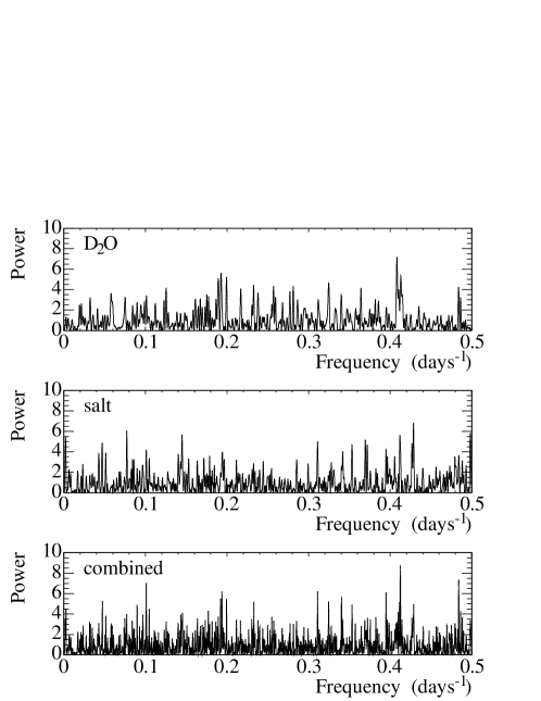
Figure 5 shows the Lomb-Scargle periodograms for the D₂O, salt, and combined data sets. A total of 7300 frequencies were tested with periods ranging from 10 years to 2 days, with a sampling step of $\Delta f=1/(14600~{}{\rm days})$ footnote2 . Because the data were binned in one-day intervals, the analysis was restricted to frequencies less than 0.5 days^-1 to avoid potential binning effects. The maximum peak height for the D₂O data set is $P=7.1$ at a period of 2.45 days ( $f=0.408$ days^-1). The largest salt peak has a height of $P=6.8$ at a period of 2.33 days ( $f=0.429$ days^-1), while the combined data set has its largest peak of $P=8.7$ at a period of 2.42 days ( $f=0.413$ days^-1).

The probability of observing a larger peak than that actually seen in the Lomb-Scargle periodogram, if the rate were constant, was estimated using the previously described 10,000 Monte Carlo data sets having no periodicity. Under the null hypothesis of no time variability, the probability of getting a peak larger than the biggest peak seen in the Lomb-Scargle periodogram is 46% for the D₂O data set, 65% for the salt data set, and 27% for the combined data sets. As with the unbinned maximum likelihood method, no evidence for time variability is seen.

III.2.2 Sensitivity to sinusoidal periodicities

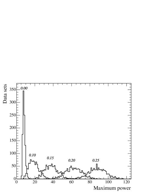
Monte Carlo data sets generated with sinusoidal periodicities were used to estimate the sensitivity of the Lomb-Scargle method to signals of various periods and amplitudes. Figure 4 shows the amplitudes as a function of frequency at which the analysis would detect the signal 50% or 90% of the time. In each case the signal is considered to be detected if the Lomb-Scargle method rejects the null hypothesis of a constant rate at the 99% confidence level. The threshold for rejecting the null hypothesis at the 99% C.L. is $P=11.15$ for the D₂O data, $P=11.43$ for the salt data, and $P=12.24$ for the combined analysis. Figure 6 shows example maximum power distributions for a 20-day period with amplitudes of 0, 10, 15, 20, and 25% for the combined analysis.

III.2.3 Systematic checks

Many checks of the Lomb-Scargle periodogram were made to verify that the results are robust. In particular, all data and Monte Carlo results were recomputed for (a) a range of bin sizes, from 1-day to 5-days in fractional day steps, (b) a range of starting times of the first bin in fractional day steps, and (c) different values of the frequency sampling step. There was no evidence for time variability under any of these scenarios.

IV Limits at Specific Frequencies of Interest

The sensitivity calculations in Sections III.1.2 and III.2.2 are appropriate when the frequency of the signal is not known a priori, and could occur anywhere in the frequency search band. The threshold for claiming a detection at the 99% C.L. must accordingly be set relatively high to reduce the false alarm probability, which was found from Monte Carlo simulations but is approximately given by integrating Equation 3 above the detection threshold, to $<1\%$ . However, if the frequency of interest is specified a priori, then a more restrictive and sensitive test can be done using the fitted amplitude at that frequency. Two particular frequencies of interest are the 7% variation in the Super-Kamiokande data at a frequency of $9.43$ y^-1 claimed by Sturrock et al. sturrock_sk3 , and the annual modulation of the neutrino flux by the Earth’s orbital eccentricity.

IV.1 Test at ${\bm{f=9.43}}$ y^-1

Sturrock et al. have claimed evidence for a periodicity in Super-Kamiokande’s neutrino data at a frequency of $9.43\pm 0.05$ y^-1 (0.0258 days^-1) with an amplitude of 7% sturrock_sk3 . Examination of SNO’s unbinned maximum likelihood results in the interval from 9.33-9.53 y^-1 yielded no value larger than $S=1.1$ in either the D₂O, the salt, or the combined data sets sk_comparison . The best-fit amplitude for the combined data set inside this frequency interval is $(1.3\pm 1.6)\%$ . This disagrees with a 7% amplitude periodicity in the ⁸B neutrino flux by 3.6 sigma. It must be remarked that SNO’s limit applies to a modulation of the summed rates of CC, ES, and NC events above their respective energy thresholds, whereas the reported 7% periodicity in the Super-Kamiokande data is a modulation of the elastic scattering rate from ⁸B neutrinos above a total electron energy threshold of 5 MeV. The best-fit amplitudes for the D₂O and salt data sets are $(3.8\pm 2.6)\%$ and $(0.3\pm 2.3)\%$ respectively.

IV.2 Eccentricity Result

The Earth’s orbital eccentricity is expected to produce a rate variation proportional, in excellent approximation, to $(1+\epsilon\cos(2\pi f(t-t_{0})))^{2}$ , where $\epsilon=0.0167$ is the eccentricity of the orbit, $f=1/(365.25~{}{\rm days})$ is the Earth’s orbital frequency, and $t_{0}$ is the time of perihelion. Maximum sensitivity to this effect is obtained if $t_{0}$ and $f$ are fixed to their known values and the combined data sets are fit for $\epsilon$ only. This has been implemented using the unbinned maximum likelihood technique. The best-fit eccentricity is $\epsilon=0.0143\pm 0.0086$ , in good agreement with the expected value. The difference in the log likelihoods for the best fit compared to $\epsilon\equiv 0$ is 1.394. The probability of obtaining a larger value of the log likelihood difference if $\epsilon=0$ is 9.5%. Figure 7 displays the relative event rate for the combined data as a function of the time since perihelion.

V Conclusions

Data from SNO’s D₂O and salt phases have been examined for time periodicities using an unbinned maximum likelihood method and the Lomb-Scargle periodogram. No evidence for any sinusoidal variation is seen in either data set or in a combined analysis of the two data sets. This general search for sinusoidal variations with periods between 1 day and 10 years has significant sensitivity to periodicities with amplitudes larger than $\sim 8\%$ . The best-fit amplitude for a sinusoidal variation in the total ⁸B neutrino flux at a frequency of 9.43 y^-1 is $(1.3\pm 1.6)$ %, which is inconsistent with the hypothesis that the results of the recent analysis by Sturrock et al. sturrock_sk3 , based on elastic scattering events in Super-Kamiokande, can be attributed to a 7% modulation of the ⁸B neutrino flux. A fit for the eccentricity of the Earth’s orbit from the modulation at a period of one year yields $\epsilon=0.0143\pm 0.0086$ , in good agreement with the known value of 0.0167.

ACKNOWLEDGMENTS

This research was supported by: Canada: Natural Sciences and Engineering Research Council, Industry Canada, National Research Council, Northern Ontario Heritage Fund, Atomic Energy of Canada, Ltd., Ontario Power Generation, High Performance Computing Virtual Laboratory, Canada Foundation for Innovation; US: Dept. of Energy, National Energy Research Scientific Computing Center; UK: Particle Physics and Astronomy Research Council. This research has been enabled by the use of WestGrid computing resources, which are funded in part by the Canada Foundation for Innovation, Alberta Innovation and Science, BC Advanced Education, and the participating research institutions. WestGrid equipment is provided by IBM, Hewlett Packard and SGI. We thank the SNO technical staff for their strong contributions. We thank Inco, Ltd. for hosting this project.

References

(1) P.A. Sturrock, Astrophys. J. 594, 1102 (2003).
(2) P.A. Sturrock, Astrophys. J. 605, 568 (2004).
(3) P.A. Sturrock et al., hep-ph/0501205.
(4) P.A. Sturrock and J.D. Scargle, Astrophys. J. 550, L101 (2001).
(5) P.A. Sturrock and D.O. Caldwell, hep-ph/0409064, submitted to Astroparticle Physics.
(6) M.A. Weber and P.A. Sturrock, Astrophys. J. 565, 1366 (2002).
(7) A. Milsztajn, hep-ph/0301252.
(8) G. Ranucci, hep-ph/0505062.
(9) J. Yoo et al., Phys. Rev. D 68, 092002 (2003).
(10) L. Pandola, Astropart. Phys. 22, 219 (2004).
(11) O.G. Miranda et al., Nucl. Phys. B 595, 360 (2001); B.C. Chauhan and J. Pulido, Phys. Rev. D 66, 053006 (2002).
(12) E.Kh. Akhmedov and J. Pulido, Phys. Lett. B 553, 7 (2003).
(13) B.C. Chauhan et al., hep-ph/0504069.
(14) The SNO Collaboration, Nucl. Instr. and Meth. A 449, 172 (2000).
(15) Q.R. Ahmad et al., Phys. Rev. Lett. 87, 071301 (2001).
(16) Q.R. Ahmad et al., Phys. Rev. Lett. 89, 011301 (2002a).
(17) Q.R. Ahmad et al., Phys. Rev. Lett. 89, 011302 (2002a).
(18) S.N. Ahmed et al., Phys. Rev. Lett. 92, 181301 (2004b).
(19) B. Aharmim et al., nucl-ex/0502021, submitted to Phys. Rev. C.
(20) N.R. Lomb, Astrophys. Space Sci. 39, 447 (1976); J.D. Scargle, Astrophys. J. 263, 835 (1982); J.D. Scargle, Astrophys. J. 343, 874 (1989).
(21) Tables of event times and run boundary times for the SNO data can be downloaded from http://sno.phy.queensu.ca/sno/periodicity/
(22) Ideally, this sample would be drawn from a Poisson distribution based on the “true” source rate, which is unknown. However, in practice, this approximation has negligible effect on the results presented here.
(23) S.S. Wilks, Ann. Math. Stat. 9, 60 (1938).
(24) K.J. Orford, Experimental Astronomy, issue 1, pp. 305-310 (1991).
(25) The calculational ease of the Lomb-Scargle analysis permitted a smaller sampling step than was used for the unbinned maximum likelihood analysis, which was CPU-intensive. We have verified that the sampling steps used for both analyses were adequate.
(26) Super-Kamiokande’s published data spans a period from May 31, 1996 to July 15, 2001, overlapping substantially with SNO’s D₂O data set. The Super-Kamiokande and SNO data sets are all entirely contained within the same solar cycle.

A Search for Periodicities in the 8B Solar Neutrino Flux Measured by the Sudbury Neutrino Observatory