2005 International Linear Collider Workshop - Stanford, U.S.A.
Trilinear Gauge Couplings from $\gamma\gamma\rightarrow W^{+}W^{-}$

Abstract

If there is no the Standard Model Higgs boson, the interaction among the gauge bosons becomes strong at high energies ($\sim 1\,{\rm TeV}$). The effects of strong electroweak symmetry breaking could manifest themselves indirectly through the vertices as anomalous gauge boson couplings before they give rise to new physical states like resonances. Here a study of the measurement of trilinear gauge couplings $\kappa_{\gamma}$ and $\lambda_{\gamma}$ is presented looking at the hadronic decay channel of the WW boson pair at an $\gamma\gamma$ - collider. A sensitivity of ${\cal O}(10^{-3}-10^{-4})$ can be reached depending on the coupling under consideration and on the initial polarisation state.

I INTRODUCTION

Deviations of the triple gauge boson couplings (TGCs) from their values predicted by the Standard Model (SM) are a possible indication for new physics (NP) beyond the SM. If no light Higgs boson exists the mechanism responsible for the restoring the unitarity could well be the strong electroweak symmetry breaking (SEWSB) mechanism strong . As a consequence, at energies below NP cut-off scale $\Lambda_{NP}$ the effects of NP are reflected in the TGC’s values leading to their deviations $\Delta\kappa_{\gamma}$ and $\Delta\lambda_{\gamma}$ from the SM predictions. Since these deviations decrease as $\Lambda_{NP}$ increases, their observation requires a very precise measurements, more precise than those at LEP and Tevatron. With a high event statistics at a $\gamma\gamma$ collider option at the International Linear Collider (ILC) it is possible to reach a high precision of the TGC measurements.

Anomalous TGCs affect both the total production cross-section and the shape of the differential cross-section as a function of the W production angle. As a consequence, distributions of W decay products are changed also. Thus, the information about TGCs can be extracted from the angular distributions of the reconstructed W boson. In $\gamma\gamma$ collisions the TGCs contribute through t-channel W-exchange.

In this study the expected sensitivity for a measurement of the couplings $\kappa_{\gamma}$ and $\lambda_{\gamma}$ in $\gamma\gamma\rightarrow W^{+}W^{-}\rightarrow 4$jets at ${\sqrt{s_{ee}}=500}\,{\rm GeV}$ ($\sqrt{s_{\gamma\gamma}}\leq 400\,{\rm GeV}$) is investigated. There are two possible initial $\gamma\gamma$ helicity states depending on the photon handedness, denoted as $J_{Z}=0$ (if two photons have the same helicities) and $|J_{Z}|=2$ (if two photons have the opposite helicities). Total and differential cross-sections distributions as a function of the anomalous TGCs ($\Delta\kappa_{\gamma},\Delta\lambda_{\gamma}\neq 0$), simulated with the tree-level Monte Carlo (MC) generator WHIZARD whizard , for all possible initial and final state helicity combinations are shown in Figures 1 and 2.

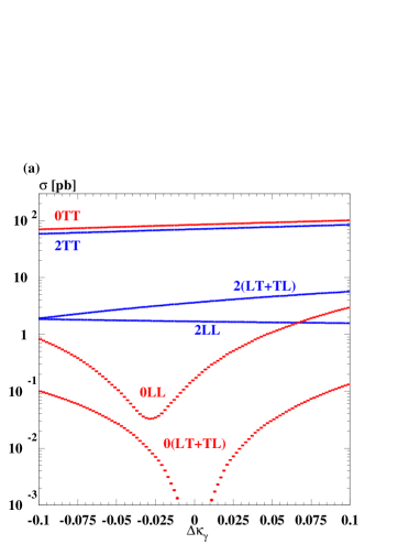
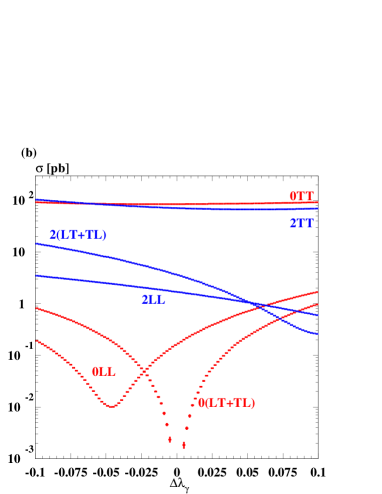
Figure 1: Contribution of different $WW$ helicity states for $J_{Z}=0$ and $|J_{Z}|=2$ states in the presence of anomalous couplings (a): ${\kappa}_{\gamma}$ and (b): ${\lambda}_{\gamma}$ at $\sqrt{s_{\gamma\gamma}}=400$ GeV, assuming fully polarised photon beams. The deviations are denoted as $\Delta\kappa_{\gamma}$ and $\Delta\lambda_{\gamma}$. The initial photon state $J_{Z}=0$ is denoted with “0” in front of helicity labelling ($LL,TT,(LT+TL)$) while the state $|J_{Z}|=2$ is denoted with “2”. TT=($\pm\pm$) for $J_{Z}=0$ and TT=($\pm\pm$)+($\pm\mp$) for $|J_{Z}|=2$. LT+TL=($\pm 0$)+($0\pm$) and LL=($00$).

II SIGNAL AND BACKGROUND SIMULATION

As a beam simulation CIRCE2 circe2 is used to describe realistic beam spectra for $\gamma\gamma$-colliders. The response of a detector has been simulated with SIMDET V4 simdet4 , a parametric Monte Carlo for the TESLA $e^{+}e^{-}$-detector. It includes a tracking and calorimeter simulation and a reconstruction of energy-flow-objects (EFO). Only the EFOs with a polar angle above $7^{\circ}$ are taken for the W boson reconstruction, simulating the acceptance of the photon collider detector as the only difference to the $e^{+}e^{-}$-detector ggparis . The signal and background events are studied on a sample of events generated with WHIZARD and overlayed with low energy ${\gamma\gamma}{\rightarrow}{\rm hadrons}$ events (pileup) thesis . The corresponding number of added pileup events per bunch crossing is 1.8 schulte . The informations about the neutral particles (neutrals) from calorimeter and charged tracks (tracks) from tracking detector are used to reconstruct the signal and background events. The potential background for both initial $J_{Z}$ states are $\gamma\gamma\rightarrow{q}{\bar{q}}$ events that can mimic the signal with four jets when gluons are radiated in the final state. The QCD corrections to the $q\bar{q}$-pair Born level production cross-section are different for the two $J_{Z}$ states: in the $|J_{Z}|=2$ state the corrected cross-section is $\sigma_{2}^{QCD}\sim\sigma_{2}^{Born}(1+k\alpha_{s}/\pi)$ with $k$ being of ${\cal O}$(1), resulting in a Born cross-section correction of 4-5$\%$. In this study this correction is not taken into account. In the $J_{Z}=0$ state, the suppression factor $(m_{f}^{2}/s)$ fadin leads to a Born level cross-section close to zero but the QCD corrections lead to an enhancement by double-logarithmic terms $\sim(\alpha_{s}\log^{2}(s/m_{q}^{2}))^{n}$ dble_log . To estimate the corrected cross-section for the $J_{Z}=0$ state the ${\cal O}(\alpha_{s}^{2})$ diagrams are taken into account i.e. the diagrams contributing to $\gamma\gamma\rightarrow q\bar{q}gg$ and $\gamma\gamma\rightarrow q\bar{q}(g\rightarrow)q\bar{q}$. The $y_{cut}$ cut parameter ($(p_{a}+p_{b})^{2}>sy_{cut}$; $a,b=q,\bar{q},g/q,g/\bar{q}$) for a variable centre-of-mass energy $s$ is defined by generating only events with the invariant masses of each parton pair above 30 GeV resulting in an emission of hard gluons. The signal events for both $J_{Z}$ states and background events for the $|J_{Z}|=2$ state are generated with O’Mega matrix element generator omega taking into account only the lowest order Feynman diagrams. The QCD correction for the $q\bar{q}$ pair production in the $J_{Z}=0$ state is estimated generating the background events with MadGraph madgraph .

II.1 Energy Flow and Event Selection

In order to minimise the pileup contribution to the high energy signal tracks, the information on the track impact parameters is used in the same way as in the case of $\gamma e$-collisions paper allowing the rejection of $\sim 60\%$ of pileup tracks and $\sim 10-15\%$ of signal tracks. The remaining tracks are combined into four jets and the events with a number of EFO greater than 40 and number of charged tracks greater than 20 are accepted only. The two reconstructed W bosons are denoted as forward ($\cos\theta>0$, $W_{F}$) and backward ($\cos\theta<0$, $W_{B}$) where $\theta$ is a W boson production angle in the centre-of-mass system (CMS). The angle between the two jets belonging to the same W boson, boosted to the CMS, is used as a next selection criteria - if the angle is within a given range of $40^{\circ}<\theta<140^{\circ}$, the event is accepted. Further, events with a total mass above 125 GeV and the individual W boson mass of $60\textrm{GeV}<M_{W}<100\textrm{GeV}$ are accepted. That results in efficiencies of approximately 53% for signal and less than 2% for background events i.e. in a purity of 81% in both $J_{Z}$ states. The top pair production is estimated to be negligible. The final angular distributions for the $|J_{Z}|=2$ state used for the TGCs error estimation are shown in Figure 3.

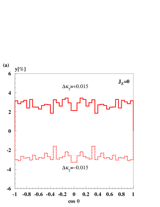
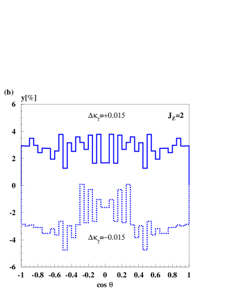
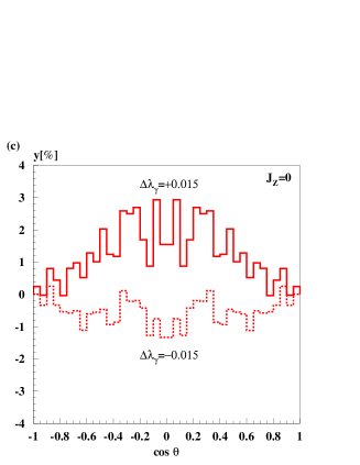
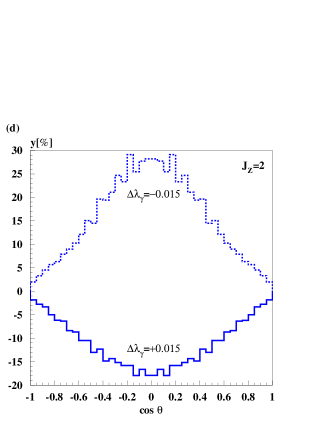
Figure 2: Relative deviations of differential cross-section from the SM predictions in presence of anomalous coupling (a): $\kappa_{\gamma}=\pm 1.015$ in the $J_{Z}=0$ state (${\Delta}{\lambda}_{\gamma}=0$), (b): $\kappa_{\gamma}=\pm 1.015$ in the $|J_{Z}|=2$ state (${\Delta}{\lambda}_{\gamma}=0$), (c): $\lambda_{\gamma}=\pm 0.015$ in the $J_{Z}=0$ state (${\Delta}{\kappa}_{\gamma}=0$) and (d): $\lambda_{\gamma}=\pm 0.015$ in the $|J_{Z}|=2$ state (${\Delta}{\kappa}_{\gamma}=0$), at $\sqrt{s_{\gamma\gamma}}=400$ GeV, assuming fully polarised photon beams. Solid lines correspond to ${\Delta}{\kappa}_{\gamma},{\Delta}{\lambda}_{\gamma}=+0.015$ and dotted lines correspond to ${\Delta}{\kappa}_{\gamma},{\Delta}{\lambda}_{\gamma}=-0.015$. All WW helicity combinations are included. $y[\%]=\frac{\left[d\sigma_{TOT}^{AC}-d\sigma_{TOT}^{SM}\right]}{d\sigma_{TOT}^{SM}}$.

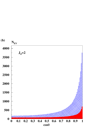
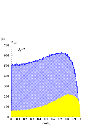
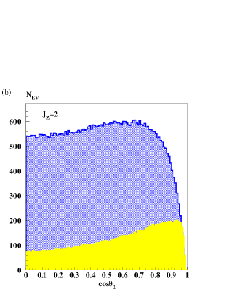
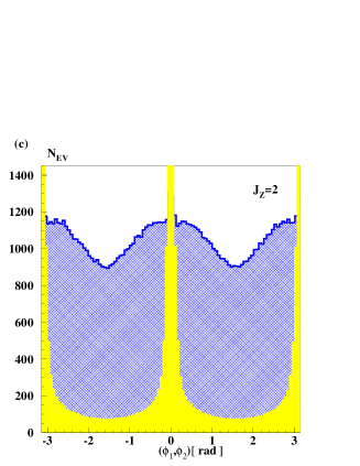
Figure 3: Angular distributions of signal (blue) and background (red, yellow) events after the detector simulation used in the fit in the $|J_{Z}|=2$ state over (a): the decay angle $\cos\theta_{1}$ of $W_{F}$ (b): the decay angle $\cos\theta_{2}$ of $W_{B}$ (c): the azimuthal angle ($\phi_{1},\phi_{2}$).

III FIT METHOD AND ERROR ESTIMATIONS

For the extraction of the TGSs from the reconstructed kinematical variables (Fig. 3) a binned Likelihood fit is used. A sample of ${2\cdot 10^{6}}$ SM signal events is generated with WHIZARD and passed trough the detector simulation. Each event is described reconstructing five kinematical variables - the W production angle with respect to the ${e^{-}}$ beam direction $\theta$, the W’s polar decay angles $\theta_{1,2}$ (angle of the fermion with respect to the W flight direction measured in the W rest frame) and the azimuthal decay angles $\phi_{1,2}$ of the fermion with respect to a plane defined by W and the beam axis. In hadronic W-decays the up- and down-type quarks cannot be separated so that only $|cos\theta_{1,2}|$ is measured. The matrix element calculations from WHIZARD are used to obtain weights paper to reweight the angular distributions as functions of the anomalous TGCs where ${\Delta}{\kappa}_{\gamma}$ and ${\lambda}_{\gamma}$ are the free parameters. Six-dimensional (6D) event distributions over $\cos{\theta}$, $\cos{\theta_{1,2}}$, $\phi_{1,2}$ and centre-of-mass energy are fitted with MINUIT min , minimising the Likelihood function depending on $\kappa_{\gamma}$ and $\lambda_{\gamma}$:

$${\cal L} = -\sum_{i,j,k,l,m,p}[z\cdot N^{SM}(i,j,k,l,m,p)\cdot\log\left(z\cdot n\cdot N^{{\Delta\kappa}_{\gamma},{\Delta\lambda}_{\gamma}}(i,j,k,l,m,p)\right)$$

$$-z\cdot n\cdot N^{{\Delta\kappa}_{\gamma},{\Delta\lambda}_{\gamma}}(i,j,k,l,m,p)]+\frac{(n-1)^{2}}{2(\Delta L^{2})},$$

where i,j,k,l and m run over the reconstructed angular distributions $\cos{\theta},\cos{\theta_{1,2}}$ and $\phi_{1,2}$, p runs over the reconstructed centre-of-mass energy, $N^{SM}(i,j,k,l,m,p)$ is the “data” which corresponds to the SM MC sample, $N^{{\Delta\kappa}_{\gamma}{\Delta\lambda}_{\gamma}}$$(i$, $j$, $k$, $l$, $m$, $p)$ (MC sample) is the event distribution weighted by the function $R({\Delta}{\kappa}_{\gamma}$,${\Delta\lambda}_{\gamma})$ and $\sigma$$(i$, $j$, $k$, $l$, $m$, $p)=\sqrt{N^{SM}(i,j,k,l,m,p)}$. The factor ${z}$ sets the number of signal events to the expected one after one year of running of an $\gamma\gamma$-collider. In case where the background is included in the fit ${z}$ defines the sum of signal and background events and ${n}\cdot N^{{\Delta\kappa}_{\gamma},{\Delta\lambda}_{\gamma}}\rightarrow[{n}\cdot N_{signal}^{{\Delta\kappa}_{\gamma},{\Delta\lambda}_{\gamma}}+N_{bck}]$. The number of background events is normalised to the effective W boson production cross-section in order to obtain the corresponding number of background events after one year of running of an $\gamma\gamma$-collider for corresponding $J_{Z}$ state. It is assumed that the total normalisation (efficiency, luminosity, electron polarisation) is only known with a relative uncertainty $\Delta L$. Thus, $n$ is taken as a free parameter in the fit and constrained to unity with the assumed normalisation uncertainty. Per construction the fit is bias-free and thus returns always exactly the SM as central values. In the $|J_{Z}|=2$ state $\Delta L=0.1\%$ is a realistic precision that can be achieved while for the $J_{Z}=0$ due to the small number of events, the luminosity is expected to be measured with an error of $\Delta L=1\%$.

Table 1 shows the estimated statistical errors we expect for the different couplings at ${\sqrt{s_{ee}}=500}\,{\rm GeV}$ for a two-parameter 6D fit at detector level including the pileup and background events in both $J_{Z}$ states.

1000 fb-1	without pileup			with pileup			pileup+background
6D fit	$J_{Z}=0/|J_{Z}|=2$			$J_{Z}=0/|J_{Z}|=2$			$J_{Z}=0/|J_{Z}|=2$
${{\Delta}L}$	1$\%$	0.1$\%$	0	1$\%$	0.1$\%$	0	1$\%$	0.1$\%$	0
${\Delta}{\kappa}_{\gamma}{\cdot}10^{-4}$	19.9/29.9	5.5/6.2	2.6/3.7	26.9/37.4	5.8/6.8	3.0/4.6	27.8/37.8	5.9/7.0	3.1/4.8
${\Delta}{\lambda}_{\gamma}{\cdot}10^{-4}$	3.7/3.1	3.7/3.1	3.7/3.1	5.4/4.6	5.2/4.6	5.2/4.6	5.7/4.8	5.6/4.8	5.6/4.8

Table 1: Estimated statistical errors for ${\kappa}_{\gamma}$ and ${\lambda}_{\gamma}$ from the 6D fit at detector level for both $J_{Z}$ states in $\gamma\gamma$ collisions at $\sqrt{s_{ee}}=500$ GeV, without pileup, with pileup and with background events.

In Table 2 the results for $\sqrt{s_{\gamma\gamma}}=400\,{\rm GeV}$ and $\sqrt{s_{\gamma\gamma}}=400\,{\rm GeV}$ are compared using a fixed photon energy.

110 fb-1	$\sqrt{s_{\gamma\gamma}}=400$ GeV						$\sqrt{s_{\gamma\gamma}}=800$ GeV
5D fit	$J_{Z}=0$			$|J_{Z}|=2$			$J_{Z}=0$			$|J_{Z}|=2$
${{\Delta}L}$	1$\%$	0.1$\%$	0	1$\%$	0.1$\%$	0	1$\%$	0.1$\%$	0	1$\%$	0.1$\%$	0
${\Delta}{\kappa}_{\gamma}{\cdot}10^{-4}$	14.4	5.4	2.6	20.1	6.2	3.8	7.2	4.5	2.4	8.1	4.6	2.6
${\Delta}{\lambda}_{\gamma}{\cdot}10^{-4}$	3.0	3.0	3.0	1.6	1.6	1.6	1.3	1.3	1.3	0.63	0.58	0.56

Table 2: Estimated statistical errors for ${\kappa}_{\gamma}$ and ${\lambda}_{\gamma}$ from the five-dimensional (5D) two-parameter fit at generator level for the $J_{Z}=0$ and $|J_{Z}|=2$ at $\gamma\gamma$ collisions at $\sqrt{s_{\gamma\gamma}}=400$ and 800 GeV. The number of events for both $J_{Z}=0$ states is normalised to the expected one with integrated luminosity of 110 fb^-1 in the high energy peak.

The comparison of $\kappa_{\gamma}$ and $\lambda_{\gamma}$ obtained from $e^{+}e^{-},\gamma e$ and $\gamma\gamma$ at $\sqrt{s_{ee}}=500$ GeV is shown in Table 3 (left side). The right side of Table 3 shows the comparison at $\sqrt{s_{e^{+}e^{-},\gamma\gamma}}=800$ GeV for the two types of collider. The sensitivities to $\kappa_{\gamma}$ and $\lambda_{\gamma}$ in $\gamma\gamma\rightarrow W^{+}W^{-}$ at $\sqrt{s_{\gamma\gamma}}=800$ GeV, including the variable energy spectrum, background and pileup events are approximated scaling the estimated sensitivities at generator level (Table 2) by a factor obtained for $\sqrt{s_{ee}}=500$ GeV. The sensitivities at an $e^{+}e^{-}$-collider are estimated at generator level.

	$\sqrt{s_{ee}}=500$ GeV					$\sqrt{s_{\gamma\gamma,e^{+}e^{-}}}=800$ GeV
LEFT	$\gamma e$	$\gamma\gamma$		$e^{+}e^{-}$	RIGHT	$\gamma\gamma$		$e^{+}e^{-}$
Mode	Real/Parasitic $|J_{Z}|=3/2$	$|J_{Z}|=2$	$J_{Z}=0$	$|J_{Z}|=1$	Mode	$|J_{Z}|=2$	$J_{Z}=0$	$|J_{Z}|=1$
$\int{\cal L}\Delta t$	160 fb-1/230 fb-1	1000 fb-1		500 fb-1	$\int{\cal L}\Delta t$	1000 fb-1
${{\Delta}L}$	0.1$\%$	0.1$\%$	1$\%$	-	${{\Delta}L}$	0.1$\%$	1$\%$	-
${\Delta}{\kappa}_{\gamma}{\cdot}10^{-4}$	10.0/11.0	7.0	27.8	3.6∗	${\Delta}{\kappa}_{\gamma}{\cdot}10^{-4}$	5.2	13.9	2.1∗
${\Delta}{\lambda}_{\gamma}{\cdot}10^{-4}$	4.9/6.7	4.8	5.7	11.0∗	${\Delta}{\lambda}_{\gamma}{\cdot}10^{-4}$	1.7	2.5	3.3∗

Table 3: Left: Comparison of the $\kappa_{\gamma}$ and $\lambda_{\gamma}$ sensitivities at $\gamma e$-, $\gamma\gamma$- and $e^{+}e^{-}$-colliders estimated at $\sqrt{s_{ee}}=500$ GeV using the polarised beams. In case of photon colliders, the background and the pileup are included. (^∗) denotes the estimation at the generator level. Right: Comparison of the $\kappa_{\gamma}$ and $\lambda_{\gamma}$ sensitivities at $\gamma\gamma$- and $e^{+}e^{-}$-colliders estimated at $\sqrt{s_{e^{+}e^{-},\gamma\gamma}}=800$ GeV using the polarised beams. (^∗) denotes the estimation at the generator level. The sensitivities at $\gamma\gamma$-collider are scaled for the background, pileup and the energy spectrum.

Concerning the systematic errors the influence of the background and the degree of photon polarisation have been investigated, assuming ${{\Delta}L}=0.1\%$ in the $|J_{Z}|=2$ state and ${{\Delta}L}=1\%$ in the $J_{Z}=0$ state. In the $J_{Z}=0$ state, the polarisation uncertainty of $0.0021$ for $\kappa_{\gamma}$ is to less than the statistical error while in the $|J_{Z}|=2$ state, the polarisation uncertainty of $0.0018$ for $\kappa_{\gamma}$ is less than three times the statistical error. The uncertainty on $\lambda_{\gamma}$ in both $J_{Z}$ states is found to be negligible. In the $|J_{Z}|=2$ state the background cross-section should be known to better than 0.8% for $\kappa_{\gamma}$ and to better than 4% for $\lambda_{\gamma}$ if the corresponding systematic uncertainty should no be larger than the statistical error. For $J_{Z}=0$ the requirement is 0.6% for $\lambda_{\gamma}$ while there are basically no restrictions for $\kappa_{\gamma}$.

IV CONCLUSIONS

The estimated sensitivity of the TGCs measurement in both $\gamma\gamma$ initial states at $\sqrt{s_{ee}}=500$ GeV with integrated luminosities of ${\cal L}_{\gamma\gamma}\approx 1000$ fb^-1 is of order $\approx 7\cdot 10^{-4}$ for $\Delta\kappa_{\gamma}$ and higher than $5\cdot 10^{-4}$ for $\Delta\lambda_{\gamma}$ in the $|J_{Z}|=2$ state assuming $\Delta L/L\approx 10^{-3}$. The state $J_{Z}=0$ takes into account a larger error on the luminosity measurement of $\Delta L/L\approx 10^{-2}$ resulting in a sensitivity to $\kappa_{\gamma}$ higher than $3\cdot 10^{-3}$ and to $\lambda_{\gamma}$ higher than $6\cdot 10^{-4}$. While $\kappa_{\gamma}$ can be measured somewhat better in $e^{+}e^{-}$, the $\gamma\gamma$-collider provides a higher accuracy for a $\lambda_{\gamma}$ measurement compared to the $e^{+}e^{-}$- and $\gamma e$-colliders.

References

• (1) M. Chanowitz, M. Golden and H. Georgi, Phys. Rev. D36 (1987) 1490; M.J.G. Veltman and F.J. Ynddurain, Nucl. Phys. B325 (1989) 1.
• (2) W. Kilian, β€œWHIZARD 1.24 A generic Monte Carlo integration and event generation package for multi-particle processes”, LC-TOOL 2001-039 (revised) (2001).
• (3) T. Ohl, β€œCirce Version 2.0: Beam Spectra for Simulating Linear Collider and Photon Collider Physics”, http://heplix.ikp.physik.tu-darmstadt.de/pub/ohl/circe2.
• (4) M.Pohl, H.J.Schreiber, β€œSIMDET-Version 4 A parametric Monte Carlo for a TESLA Detector”, DESY 02-061, May 2002.
• (5) K. MΓΆnig, β€œA Photon Collider at TESLA”, LC-DET-2004-014 (2004).
• (6) D. Schulte, β€œStudy of Electromagnetic and Hadronic Background in the Interaction Region of the TESLA Collider”, Thesis, April 1997.
• (7) D. Schulte, private communication.
• (8) V.S. Fadin, V.A. Khoze and A.D. Martin, Phys. Rev. D56 (1997) 484-503.
• (9) M. Melles and W.J. Stirling, Phys. Rev. D59 (1999) 094009.
• (10) M. Moretti, T. Ohl and J. Reuter, LC-TOOL-2001-040 (2001).
• (11) T. Stelzer and W.F. Long, Comput. Phys. Commun.81 (1994) 357.
• (12) K. MΓΆnig and J. Sekaric, Eur. Phys. J.C. 38 (2005) 427-436.
• (13) F.James, MINUIT Function Minimization and Error Analysis, Version 94.1, CERN Program Library Long Writeup D506.