EUROPEAN ORGANISATION FOR NUCLEAR RESEARCH

CERN-PH-EP/2005-024

13 June, 2005

Determination of $\alpha_{\rm{s}}$ Using Jet Rates at LEP with the OPAL Detector

The OPAL Collaboration

Abstract:

Hadronic events produced in $\mathrm{e}^{+}\mathrm{e}^{-}$ collisions by the LEP collider and recorded by the OPAL detector were used to form distributions based on the number of reconstructed jets. The data were collected between 1995 and 2000 and correspond to energies of 91 GeV, 130-136 GeV and 161-209 GeV. The jet rates were determined using four different jet-finding algorithms (Cone, JADE, Durham and Cambridge). The differential two-jet rate and the average jet rate with the Durham and Cambridge algorithms were used to measure $\alpha_{\rm{s}}$ in the LEP energy range by fitting an expression in which $\mathcal{O}(\mbox{$\alpha_{\rm{s}}^{2}$})$ calculations were matched to a NLLA prediction and fitted to the data. Combining the measurements at different centre-of-mass energies, the value of $\alpha_{\rm{s}}$($M_{\mathrm{Z}}$) was determined to be

$\alpha_{\rm{s}}$($M_{\mathrm{Z}}$)=$0.1177\pm 0.0006$(stat.)$\pm 0.0012$(expt.)$\pm 0.0010$(had.)$\pm 0.0032$(theo.).

(Submitted to European Physical Journal C)

The OPAL Collaboration

G. Abbiendi², C. Ainsley⁵, P.F. Åkesson^3,y, G. Alexander²², G. Anagnostou¹, K.J. Anderson⁹, S. Asai²³, D. Axen²⁷, I. Bailey²⁶, E. Barberio^8,p, T. Barillari³², R.J. Barlow¹⁶, R.J. Batley⁵, P. Bechtle²⁵, T. Behnke²⁵, K.W. Bell²⁰, P.J. Bell¹, G. Bella²², A. Bellerive⁶, G. Benelli⁴, S. Bethke³², O. Biebel³¹, O. Boeriu¹⁰, P. Bock¹¹, M. Boutemeur³¹, S. Braibant², R.M. Brown²⁰, H.J. Burckhart⁸, S. Campana⁴, P. Capiluppi², R.K. Carnegie⁶, A.A. Carter¹³, J.R. Carter⁵, C.Y. Chang¹⁷, D.G. Charlton¹, C. Ciocca², A. Csilling²⁹, M. Cuffiani², S. Dado²¹, A. De Roeck⁸, E.A. De Wolf^8,s, K. Desch²⁵, B. Dienes³⁰, M. Donkers⁶, J. Dubbert³¹, E. Duchovni²⁴, G. Duckeck³¹, I.P. Duerdoth¹⁶, E. Etzion²², F. Fabbri², P. Ferrari⁸, F. Fiedler³¹, I. Fleck¹⁰, M. Ford¹⁶, A. Frey⁸, P. Gagnon¹², J.W. Gary⁴, C. Geich-Gimbel³, G. Giacomelli², P. Giacomelli², M. Giunta⁴, J. Goldberg²¹, E. Gross²⁴, J. Grunhaus²², M. Gruwé⁸, P.O. Günther³, A. Gupta⁹, C. Hajdu²⁹, M. Hamann²⁵, G.G. Hanson⁴, A. Harel²¹, M. Hauschild⁸, C.M. Hawkes¹, R. Hawkings⁸, R.J. Hemingway⁶, G. Herten¹⁰, R.D. Heuer²⁵, J.C. Hill⁵, D. Horváth^29,c, P. Igo-Kemenes¹¹, K. Ishii²³, H. Jeremie¹⁸, P. Jovanovic¹, T.R. Junk^6,i, J. Kanzaki^23,u, D. Karlen²⁶, K. Kawagoe²³, T. Kawamoto²³, R.K. Keeler²⁶, R.G. Kellogg¹⁷, B.W. Kennedy²⁰, S. Kluth³², T. Kobayashi²³, M. Kobel³, S. Komamiya²³, T. Krämer²⁵, A. Krasznahorkay^30,e, P. Krieger^6,l, J. von Krogh¹¹, T. Kuhl²⁵, M. Kupper²⁴, G.D. Lafferty¹⁶, H. Landsman²¹, D. Lanske¹⁴, D. Lellouch²⁴, J. Letts^o, L. Levinson²⁴, J. Lillich¹⁰, S.L. Lloyd¹³, F.K. Loebinger¹⁶, J. Lu^27,w, A. Ludwig³, J. Ludwig¹⁰, W. Mader^3,b, S. Marcellini², A.J. Martin¹³, T. Mashimo²³, P. Mättig^m, J. McKenna²⁷, R.A. McPherson²⁶, F. Meijers⁸, W. Menges²⁵, F.S. Merritt⁹, H. Mes^6,a, N. Meyer²⁵, A. Michelini², S. Mihara²³, G. Mikenberg²⁴, D.J. Miller¹⁵, W. Mohr¹⁰, T. Mori²³, A. Mutter¹⁰, K. Nagai¹³, I. Nakamura^23,v, H. Nanjo²³, H.A. Neal³³, R. Nisius³², S.W. O’Neale^1,∗, A. Oh⁸, M.J. Oreglia⁹, S. Orito^23,∗, C. Pahl³², G. Pásztor^4,g, J.R. Pater¹⁶, J.E. Pilcher⁹, J. Pinfold²⁸, D.E. Plane⁸, O. Pooth¹⁴, M. Przybycień^8,n, A. Quadt³, K. Rabbertz^8,r, C. Rembser⁸, P. Renkel²⁴, J.M. Roney²⁶, A.M. Rossi², Y. Rozen²¹, K. Runge¹⁰, K. Sachs⁶, T. Saeki²³, E.K.G. Sarkisyan^8,j, A.D. Schaile³¹, O. Schaile³¹, P. Scharff-Hansen⁸, J. Schieck³², T. Schörner-Sadenius^8,z, M. Schröder⁸, M. Schumacher³, R. Seuster^14,f, T.G. Shears^8,h, B.C. Shen⁴, P. Sherwood¹⁵, A. Skuja¹⁷, A.M. Smith⁸, R. Sobie²⁶, S. Söldner-Rembold¹⁶, F. Spano⁹, A. Stahl^3,x, D. Strom¹⁹, R. Ströhmer³¹, S. Tarem²¹, M. Tasevsky^8,s, R. Teuscher⁹, M.A. Thomson⁵, E. Torrence¹⁹, D. Toya²³, P. Tran⁴, I. Trigger⁸, Z. Trócsányi^30,e, E. Tsur²², M.F. Turner-Watson¹, I. Ueda²³, B. Ujvári^30,e, C.F. Vollmer³¹, P. Vannerem¹⁰, R. Vértesi^30,e, M. Verzocchi¹⁷, H. Voss^8,q, J. Vossebeld^8,h, C.P. Ward⁵, D.R. Ward⁵, P.M. Watkins¹, A.T. Watson¹, N.K. Watson¹, P.S. Wells⁸, T. Wengler⁸, N. Wermes³, G.W. Wilson^16,k, J.A. Wilson¹, G. Wolf²⁴, T.R. Wyatt¹⁶, S. Yamashita²³, D. Zer-Zion⁴, L. Zivkovic²⁴

¹School of Physics and Astronomy, University of Birmingham, Birmingham B15 2TT, UK
²Dipartimento di Fisica dell’ Università di Bologna and INFN, I-40126 Bologna, Italy
³Physikalisches Institut, Universität Bonn, D-53115 Bonn, Germany
⁴Department of Physics, University of California, Riverside CA 92521, USA
⁵Cavendish Laboratory, Cambridge CB3 0HE, UK
⁶Ottawa-Carleton Institute for Physics, Department of Physics, Carleton University, Ottawa, Ontario K1S 5B6, Canada
⁸CERN, European Organisation for Nuclear Research, CH-1211 Geneva 23, Switzerland
⁹Enrico Fermi Institute and Department of Physics, University of Chicago, Chicago IL 60637, USA
¹⁰Fakultät für Physik, Albert-Ludwigs-Universität Freiburg, D-79104 Freiburg, Germany
¹¹Physikalisches Institut, Universität Heidelberg, D-69120 Heidelberg, Germany
¹²Indiana University, Department of Physics, Bloomington IN 47405, USA
¹³Queen Mary and Westfield College, University of London, London E1 4NS, UK
¹⁴Technische Hochschule Aachen, III Physikalisches Institut, Sommerfeldstrasse 26-28, D-52056 Aachen, Germany
¹⁵University College London, London WC1E 6BT, UK
¹⁶Department of Physics, Schuster Laboratory, The University, Manchester M13 9PL, UK
¹⁷Department of Physics, University of Maryland, College Park, MD 20742, USA
¹⁸Laboratoire de Physique Nucléaire, Université de Montréal, Montréal, Québec H3C 3J7, Canada
¹⁹University of Oregon, Department of Physics, Eugene OR 97403, USA
²⁰CCLRC Rutherford Appleton Laboratory, Chilton, Didcot, Oxfordshire OX11 0QX, UK
²¹Department of Physics, Technion-Israel Institute of Technology, Haifa 32000, Israel
²²Department of Physics and Astronomy, Tel Aviv University, Tel Aviv 69978, Israel
²³International Centre for Elementary Particle Physics and Department of Physics, University of Tokyo, Tokyo 113-0033, and Kobe University, Kobe 657-8501, Japan
²⁴Particle Physics Department, Weizmann Institute of Science, Rehovot 76100, Israel
²⁵Universität Hamburg/DESY, Institut für Experimentalphysik, Notkestrasse 85, D-22607 Hamburg, Germany
²⁶University of Victoria, Department of Physics, P O Box 3055, Victoria BC V8W 3P6, Canada
²⁷University of British Columbia, Department of Physics, Vancouver BC V6T 1Z1, Canada
²⁸University of Alberta, Department of Physics, Edmonton AB T6G 2J1, Canada
²⁹Research Institute for Particle and Nuclear Physics, H-1525 Budapest, P O Box 49, Hungary
³⁰Institute of Nuclear Research, H-4001 Debrecen, P O Box 51, Hungary
³¹Ludwig-Maximilians-Universität München, Sektion Physik, Am Coulombwall 1, D-85748 Garching, Germany
³²Max-Planck-Institute für Physik, Föhringer Ring 6, D-80805 München, Germany
³³Yale University, Department of Physics, New Haven, CT 06520, USA

^a and at TRIUMF, Vancouver, Canada V6T 2A3
^b now at University of Iowa, Dept of Physics and Astronomy, Iowa, U.S.A.
^c and Institute of Nuclear Research, Debrecen, Hungary
^e and Department of Experimental Physics, University of Debrecen, Hungary
^f and MPI München
^g and Research Institute for Particle and Nuclear Physics, Budapest, Hungary
^h now at University of Liverpool, Dept of Physics, Liverpool L69 3BX, U.K.
ⁱ now at Dept. Physics, University of Illinois at Urbana-Champaign, U.S.A.
^j and Manchester University Manchester, M13 9PL, United Kingdom
^k now at University of Kansas, Dept of Physics and Astronomy, Lawrence, KS 66045, U.S.A.
^l now at University of Toronto, Dept of Physics, Toronto, Canada
^m current address Bergische Universität, Wuppertal, Germany
ⁿ now at University of Mining and Metallurgy, Cracow, Poland
^o now at University of California, San Diego, U.S.A.
^p now at The University of Melbourne, Victoria, Australia
^q now at IPHE Université de Lausanne, CH-1015 Lausanne, Switzerland
^r now at IEKP Universität Karlsruhe, Germany
^s now at University of Antwerpen, Physics Department,B-2610 Antwerpen, Belgium; supported by Interuniversity Attraction Poles Programme – Belgian Science Policy
^u and High Energy Accelerator Research Organisation (KEK), Tsukuba, Ibaraki, Japan
^v now at University of Pennsylvania, Philadelphia, Pennsylvania, USA
^w now at TRIUMF, Vancouver, Canada
^x now at DESY Zeuthen
^y now at CERN
^z now at DESY
^∗ Deceased

1 Introduction

In the Standard Model of elementary particle interactions, the strong interaction is described by the theory of Quantum Chromodynamics (QCD), and depends on just one fundamental parameter, the strong coupling $\alpha_{\rm{s}}$. The value of $\alpha_{\rm{s}}$ is expected to depend on the energy scale of the interaction. It is therefore an important test of the theory to determine the value of $\alpha_{\rm{s}}$ experimentally at as many different energies as possible. It is also important to use as many different techniques as possible, as different measurements of $\alpha_{\rm{s}}$ are sensitive to different theoretical and hadronization variations.

Indeed, many methods have already been employed to evaluate $\alpha_{\rm{s}}$ [1]. At very low energies the value of $\alpha_{\rm{s}}$ can be measured using the hadronic decays of the $\tau$ lepton and heavy quarkonia. Low energy determinations are also available using scaling violations and sum rules from deep inelastic scattering experiments. Higher energy determinations of $\alpha_{\rm{s}}$ come from collider experiments ($\mathrm{e}^{+}\mathrm{e}^{-}$ ​​​, pp, p$\bar{\rm{p}}$ or ep) using properties of the created hadron system which are explicitly dependent on the value of $\alpha_{\rm{s}}$($Q$), where $Q$ corresponds to the energy scale at which the interaction takes place.

During the LEP1.5 ($\sqrt{s}$ $\sim$133 GeV) and LEP2 (above $\mathrm{W}^{+}\mathrm{W}^{-}$ threshold) operational phases of the Large Electron-Positron collider at CERN, events were recorded with centre-of-mass collision energies ranging from 91 GeV to 209 GeV. Events of the form $\mathrm{e}^{+}\mathrm{e}^{-}$ $\rightarrow$hadrons can be used to determine distributions based on the ensemble of final state hadrons (event shapes) or on the ensemble of jets (jet rates). Previous results by OPAL for an $\alpha_{\rm{s}}$ determination based on event shapes and jet rates using the $\mathrm{Z}$ dataset collected during the LEP1 phase can be found in [2]. Determinations of $\alpha_{\rm{s}}$ from LEP1.5 and LEP2 datasets up to 189 GeV have already been reported by OPAL based on event shape distributions [3, 4, 5] and on jet rates [6]. Another OPAL paper [7] uses the same data that have been presented here to measure event shapes.

For the analysis presented in this paper we used data collected during the LEP1.5 and LEP2 phases to construct jet rate distributions using several jet clustering algorithms. The differential two-jet rate, $D_{2}$, and the average jet rate, $\langle N\rangle$, were used to determine values of $\alpha_{\rm{s}}$($\sqrt{s}$) at the four combined centre-of-mass energies composed of data within the LEP1.5 and LEP2 datasets. Theoretical predictions were fitted to these distributions to extract the value of $\alpha_{\rm{s}}$($\sqrt{s}$).

The paper is organized as follows. Section 2 contains a brief description of the OPAL detector. A summary of the data and the Monte Carlo samples used in the analysis is given in Section 3. In Section 4, we define the jet rate distributions. The methods used to select signal events and reject backgrounds are presented in Section 5. The variations used for systematic studies are detailed in Section 6. Finally, the results of this analysis are given in Section 7, followed by a conclusion and summary in Section 8.

2 The OPAL Experiment

A full description of the OPAL detector can be found in [8]. The critical components of the detector in the identification of jets were the central tracking chambers, which were used to reconstruct charged particles, and the electromagnetic calorimeters, which measured the total energy deposited by electrons and photons.

The tracking chambers were located inside a solenoidal magnet which provided a 0.435 T axial magnetic field along the beam axis. The main component of the tracking system was a large-volume jet chamber, which was approximately 4.0 m long with an outer radius of 1.85 m. The jet chamber was separated into 24 sectors, each with a radial plane of 159 sense wires separated by 1 cm. The momenta of tracks in the $x-y$ plane were measured with a precision parametrized by $\sigma_{p}/p=\sqrt{0.02^{2}+(0.0015\cdot p[\rm{GeV}/\mathit{c}])^{2}}$.

The calorimetry systems were outside the solenoidal magnet. The electromagnetic calorimeter was composed of 11704 lead glass blocks in the barrel and endcap regions, representing about 25 radiation lengths in the barrel and more than 22 in the endcap. The iron sampling hadron calorimeter was located just outside the electromagnetic calorimeter, and provided the stopping power to contain most hadronic showers. Luminosity was determined using small-angle Bhabha events detected in the forward detectors and silicon-tungsten calorimeter [9].

After an event was triggered [10], data were collected from the subdetectorsand processed by the OPAL data acquisition system [11]. The raw event data were transferred to a farm of computer processors where the events were fully reconstructed and written to tape for offline analysis.

3 Data and Monte Carlo Samples

The data used in this analysis were collected by OPAL between 1995 and 2000 and correspond to integrated luminosities of 14.7 pb^-1 of data taken with centre-of-mass energy 91 GeV, 11.3 pb^-1 of LEP1.5 data with centre-of-mass energies between 130 GeV and 136 GeV and 707.4 pb^-1 of LEP2 data with centre-of-mass energies ranging from 161 to 209 GeV. The 91 GeV data, known as $\mathrm{Z}$-calibration data, were primarily collected for calibrating parameters used in the OPAL reconstruction algorithms. This $M_{\mathrm{Z}}$ sample had the same detector configuration as the other centre-of-mass energy points. The exact breakdown of the centre-of-mass energies together with the respective luminosities and numbers of selected events are given in Table 1. The thirteen points in Table 1 represent the main samples of the spread of energies in the LEP1.5 and LEP2 data.

The data were combined into four datasets. The LEP1.5 data provided a single energy point at an event-weighted centre-of-mass energy of 133 GeV, while the LEP2 data were split into two energy points, one with an event-weighted centre-of-mass energy of 177 GeV using data in the range 161–185 GeV (with a total integrated luminosity of 78.1 pb^-1) and another at 197 GeV (with a total integrated luminosity of 628.3 pb^-1) using data in the range 188–209 GeV. Together with the $\mathrm{Z}$-calibration data this provided for a determination of $\alpha_{\rm{s}}$ at four centre-of-mass energies.

A number of Monte Carlo samples were created to correct for detector acceptance and resolution effects, to correct for hadronization effects and to estimate the contribution of background processes. These Monte Carlo samples were produced using a full simulation of the detector [12], followed by the same reconstruction and selection algorithms applied to the real data, and are referred to as “detector-level” samples. Other samples without the full detector simulation are discussed in Section 5.2.

PYTHIA 6.150 [13] was used to provide the default Monte Carlo samples (for the process $\mathrm{e}^{+}\mathrm{e}^{-}$ $\rightarrow\rm{Z}/\gamma^{\ast}\rightarrow\$$\mathrm{q}\overline{\mathrm{q}}$ $\rightarrow$ hadrons) which were used to correct the high energy datasets. The $\mathrm{Z}$-calibration dataset was corrected using JETSET 7.408 [14]. The use of JETSET for the lower energy data is a matter of convenience only, and not due to any inconsistencies in PYTHIA at this energy. Any differences between the two generators is expected to be negligible. Hadronization corrections were evaluated by comparing results with an alternative Monte Carlo sample, HERWIG 6.2 [15] which uses the cluster model of hadronization. This was compared with the string model of hadronization in PYTHIA. The parameters which were involved in the Monte Carlo simulation, both for JETSET/PYTHIA and HERWIG, were tuned to OPAL data collected at the $\mathrm{Z}$ peak, including global event shapes, particle multiplicities and fragmentation functions [16, 17]. The generation of the initial quark-antiquark pair for each Monte Carlo sample was implemented at LEP2 using the $\mathcal{KK}$2f 4.13 event generator [18], which has an improved description of photon production in the initial and final states with respect to the one currently implemented in the PYTHIA generator. The available detector-level Monte Carlo samples are listed in Table 1.

Above the $\mathrm{W}^{+}\mathrm{W}^{-}$ production threshold (161 GeV), the main background was expected to come from four-fermion events ($\mathrm{e}^{+}\mathrm{e}^{-}$ $\rightarrow$$\rm{W}^{+}\rm{W}^{-}$$\rightarrow$4f), in particular those events in which two or all four of the fermions were quarks. The contribution of these backgrounds in data was estimated using Monte Carlo samples generated using KORALW 1.42 [19] (for q$\bar{\rm{q}}$q${}^{\prime}\bar{\rm{q}}^{\prime}$ and q$\bar{\rm{q}}\ell\bar{\ell}^{(\prime)}$ where $\ell=\mathrm{e},\mu,\tau,\nu$ but $\ell\bar{\ell}\neq\mathrm{e}^{+}\mathrm{e}^{-}$) and grc4f 2.1 [20] (for eeq$\bar{\rm{q}}$). Grc4f 2.1 was used to generate all the expected four-fermion background samples for the 161 and 172 GeV data. The background distributions were normalized to the luminosity of the dataset and subsequently subtracted from the measured distributions. The LEP1.5 energies were well below the $\mathrm{W}^{+}\mathrm{W}^{-}$ and $\rm{Z}\rm{Z}$ production thresholds [21] and were therefore expected to have no significant four-fermion backgrounds. The total expected background contribution from “four-fermion” $\mathrm{e^{+}e^{-}}\rightarrow\mathrm{q\overline{q}q\overline{q}}$ events is 1.2% of the combined LEP1.5 data sample and it was neglected in the analysis.

4 Jet Rate Distributions

Jets were formed from the final state objects by applying jet clustering algorithms. These algorithms use the kinematic and spatial (geometric) properties of the individual objects in order to classify them as belonging to a specific jet. We used here the Durham [22], Cambridge [23], JADE [24] and the $R$ and $\varepsilon$ variants of the Cone [25] jet clustering algorithms.

The Durham and Cambridge algorithms construct a test variable built from the energy and angular separation between two particles,

$$y_{ij}=\frac{2\min\{E_{i}^{2},E_{j}^{2}\}(1-\cos\theta_{ij})}{E_{\rm{vis}}^{2}}$$

where $E_{i}$ is the energy of particle $i$, $\theta_{ij}$ the angle between the particle $i$ and $j$ and $E_{\rm{vis}}$ is the total visible energy in the event. The pair that produces the smallest value of $y_{ij}$ is chosen first. The value of this test variable is compared to a predefined parameter, $y_{\rm{cut}}$, called the jet resolution parameter. If the test variable is smaller than $y_{\rm{cut}}$ particles $i$ and $j$ are merged into a pseudo-particle. Merging means that the momenta of particles $i$ and $j$ are removed from the set of momenta and the the sum of their four-momenta is added to the set of momenta. After the merging, the clustering starts again using the momentum set and it continues until all test variables become larger than $y_{\rm{cut}}$. After the clustering stops, all remaining (pseudo-) particles are classified as jets.

The Cambridge algorithm differs slightly from Durham in its implementation. In the Cambridge algorithm particles are first paired together by minimizing the variable $v_{ij}=2(1-\cos\theta_{ij})$. The standard test variable is then constructed and compared to the jet resolution parameter, $y_{\rm{cut}}$. The procedure followed is then identical to that of the Durham algorithm, except that Cambridge freezes out soft jets by accepting only the lowest energy (pseudo-)particle as the jet when $y_{ij}>\mbox{$y_{\rm{cut}}$}$. The number of jets reconstructed in the event, using Durham or Cambridge, is therefore a function of the jet resolution parameter. The JADE algorithm follows the same procedure as the Durham algorithm; however, it uses the scaled invariant mass, $y_{ij}=2E_{i}E_{j}(1-\cos\theta_{ij})/E_{\rm{vis}}^{2}$, of particles $i$ and $j$ as the test variable.

In the Cone jet finding algorithm, a jet is defined as a set of particles whose three-momentum vectors lie inside a cone of half angle $R$, where the direction of the sum of their three-momentum vectors defines the cone axis. In addition, the total energy of the particles assigned to a jet is required to exceed some minimum value $\varepsilon$. Typical values are $R=0.7$ rad and $\varepsilon=7$ GeV for jets in $\mathrm{e}^{+}\mathrm{e}^{-}$ annihilation at LEP 1 energies. When analysing events at the detector level, we replaced $\varepsilon$ by $\varepsilon^{\prime}=\varepsilon\cdot E_{\rm{vis}}/$$\sqrt{s}$ to compensate for the incomplete detection of the energy of the event. In our studies, the jet rate was computed at fixed $\varepsilon=7$ GeV as $R$ was varied, and at fixed $R=0.7$ as $\varepsilon$ was varied. The former is sensitive to the angular structure of jets, and the latter to their energy distribution.

The fraction of multihadronic events in a given sample that are classified as containing $n$ jets for a given value of the jet resolution parameter ($y_{\rm{cut}}$, $R$ or $\varepsilon$) is referred to as the $n$-jet rate. This $n$-jet rate is explicitly defined as

$$R_{n}(\mbox{$y_{\rm{cut}}$})=\frac{\sigma_{n}(\mbox{$y_{\rm{cut}}$})}{\sigma_{\rm{tot}}}\equiv\frac{N_{n}(\mbox{$y_{\rm{cut}}$})}{N_{\rm{tot}}},$$ (1)

where $\sigma_{n}$ is the cross-section for the production of a hadronic event with $n$ jets at fixed $y_{\rm{cut}}$, $\sigma_{tot}$ is the total hadronic cross-section, $N_{n}(\mbox{$y_{\rm{cut}}$})$ is the number of events in a sample with $n$ jets for a given value of $y_{\rm{cut}}$ and $N_{tot}$ is the total number of events in that sample.

The differential $n$-jet rate was also determined. It is the derivative of the $n$-jet rate with respect to $y_{\rm{cut}}$,

$$D_{n}(\mbox{$y_{\rm{cut}}$}) = \frac{\mathrm{d}R_{n}(\mbox{$y_{\rm{cut}}$})}{\rm{d}\mbox{$y_{\rm{cut}}$}}.$$ (2)

For the case when $n=2$, the differential 2-jet rate reduces to $D_{2}=y_{23}$, where $y_{23}$ is the value of the jet resolution parameter where the event flips from a 2- to a 3-jet event. When the Durham algorithm is used to define jets the value of $D_{2}$ (denoted $y_{23}^{D}$) is also an event shape variable.

The average number of jets per event in a given sample, as a function of the jet resolution parameter, is defined to be

$$\langle N\rangle(\mbox{$y_{\rm{cut}}$}) = \frac{1}{\sigma_{\rm{tot}}}\sum_{n}n\sigma_{n}(\mbox{$y_{\rm{cut}}$})$$ (3)

$$= \frac{1}{N_{\rm{tot}}}\sum_{n}nN_{n}(\mbox{$y_{\rm{cut}}$}).$$

A QCD prediction which matches an $\mathcal{O}(\mbox{$\alpha_{\rm{s}}^{2}$})$ (next-leading order) prediction, based on the QCD matrix elements [26], with a resummed, next-leading logarithmic approximation (NLLA) [27] prediction, such that terms that appear in both predictions are not double counted, was fitted to data. In this analysis we used the $\ln R$ matched $D_{2}$ [28, 29, 22] and $\langle N\rangle$ [6, 30] predictions to fit to the distributions of the observables. The differential and average jet rates were determined using the Durham and Cambridge clustering algorithms, since resummed predictions only exist for these algorithms. This provided four separate observables ($D_{2}^{D}$, $D_{2}^{C}$, $\langle N\rangle^{D}$ and $\langle N\rangle^{C}$) which were used to determine a value of $\alpha_{\rm{s}}$ at the four different centre-of-mass energy values.

5 Analysis Procedure

5.1 Selection Method

5.1.1 Preselection

All events within a dataset were required to contain information from both the central jet chamber and the electromagnetic calorimeter, meaning both these subdetectors must have been flagged as being on and in good operational condition. In addition events were required to be tagged as multihadronic in order to be preselected for analysis. Multihadronic events were identified using the criteria described in [31] for events with $\sqrt{s}$ $>$$M_{\mathrm{Z}}$ and in [32] for $\mathrm{Z}$-calibration events. To pass the preselection, an event was required to contain at least seven good tracks to reduce potential backgrounds arising from the production of $\tau$ leptons ($\mathrm{e}^{+}\mathrm{e}^{-}$ $\rightarrow\tau^{+}\tau^{-}$) decaying into hadrons and from two-photon interactions producing quarks. Good tracks were defined as those which had

• at least 40 hits in the jet chamber

• at least 150 MeV/$c$ transverse momentum relative to the beam axis.

• the distance of closest approach to the interaction point in the $r-\phi$ plane satisfying $d_{0}\leq 2$ cm

• the point of closest approach $\leq 25$ cm from the interaction point in the $z$-direction

Clusters of energy in the calorimeters were also used in the analysis; good clusters were defined as those which produced a signal in at least one block in the barrel electromagnetic calorimeter corresponding to an uncorrected energy of at least 100 MeV or of 2 blocks in the endcap electromagnetic calorimeter corresponding to an uncorrected energy of 250 MeV. The hadron calorimeter was not used in this analysis.

All of the good quality tracks and clusters in the event were used to define “objects” representing particles using an algorithm (MT) to correct for double counting of energy. This MT algorithm produced a uniquely defined array of track and cluster objects. The trajectories of the tracks measured in the central tracking chambers were extrapolated to the clusters in the electromagnetic calorimeters. If the energy of the cluster was less than expected from the track, then the cluster was omitted to avoid double counting of energy, since the momentum resolution for tracks was typically better than the calorimeter energy resolution. If the energy of the cluster was larger than expected the energy of the cluster was reduced by the expected amount with the remaining energy interpreted as due to photons or neutral hadrons. These remaining clusters and those which were not matched defined the four-vectors of “neutral” particles. In all cases tracks were treated as charged pions and neutral particles were treated as being massless.

5.1.2 Containment

We ensured that most particles in the event were well contained in the detector and not lost down the beam line by imposing a cut on the direction of the thrust axis [33],

• $|\cos\theta_{\rm{T}}|<0.9$,

where $\theta_{\rm{T}}$ is the angle between the beam axis and the direction of the thrust axis. The thrust axis direction was determined from all tracks and clusters in the event, without correcting for double counting with the MT algorithm.

5.1.3 Initial State Radiation (ISR) Cuts

The events of interest for this analysis were $\mathrm{e^{+}e^{-}}\rightarrow\mathrm{q\overline{q}}$ events where the final-state $\mathrm{q}\overline{\mathrm{q}}$ pair had the full centre-of-mass energy. The effective centre-of-mass energy of the $\mathrm{e}^{+}\mathrm{e}^{-}$ collision can be reduced by the emission of one or more ISR photons. At LEP2, approximately three quarters of the multihadronic events were such “radiative return events”, where the invariant mass of the $\mathrm{q}\overline{\mathrm{q}}$ pair was close to the $\mathrm{Z}$ mass. The effective centre-of-mass energy of the collision after ISR, $\sqrt{s^{\prime}}$ [34], was evaluated, and the requirement

• $\sqrt{s}-\sqrt{s^{\prime}}<$10 GeV

was imposed to select full-energy events.

To calculate $\sqrt{s^{\prime}}$, all isolated photon candidates with energies greater than 10 GeV were identified. The Durham jet reconstruction algorithm [31] was then used to group the remaining tracks and clusters into jets. ISR photons are often emitted close to the beam direction. Three kinematic fits were performed, under the assumptions that

• there were two undetected photons (in opposite directions along the beam pipe)

• there was one undetected photon

• all photons were observed in the detector,

respectively. The fit with the most acceptable $\chi^{2}$ was selected, and $\sqrt{s^{\prime}}$ was calculated from the invariant mass of the jets, excluding any photons.

The power of this cut can be seen in Figure 1. The efficiency for selecting non-radiative $\mathrm{q}\overline{\mathrm{q}}$ events is given in Table 2. The purity of non-radiative events was found to be approximately 73% in all of the LEP1.5 and LEP2 data samples. Non-radiative $\mathrm{q}\overline{\mathrm{q}}$ events are defined as those in which $\sqrt{s}-\sqrt{s^{\prime}_{\rm{true}}}<1$ GeV, where $s^{\prime}_{\rm{true}}$ was determined from generator-level information in the PYTHIA samples. This ISR cut was applied to all analyzed datasets with the exception of the $\mathrm{Z}$ calibration data.

5.1.4 Final Cuts

The dominant background to the process $\mathrm{e}^{+}\mathrm{e}^{-}$ $\rightarrow\rm{Z}/\gamma^{\ast}\rightarrow$ $\mathrm{q}\overline{\mathrm{q}}$ $\rightarrow$ hadrons at LEP2 came from the four-fermion process $\mathrm{e}^{+}\mathrm{e}^{-}$ $\rightarrow$$\rm{W}^{+}\rm{W}^{-}$ in which one or both of the bosons decayed hadronically, producing two or four quarks in the final state. This background was expected to make up approximately 30% of all observed events which pass the first stage of cuts in each of the LEP2 datasets. These backgrounds were addressed by placing a cut [35] on two likelihood values which indicate how likely an event is to be a non-QCD four-quark or a semi-leptonic event:

• $\mathcal{L}$${}_{\mathrm{q}\overline{\mathrm{q}}\mathrm{q}\overline{\mathrm{q}}}$ $<0.25$

• $\mathcal{L}$${}_{\mathrm{q}\overline{\mathrm{q}}\ell\nu}$ $<0.50$

The effect of these cuts in each of the LEP2 datasets and the expected backgrounds can be seen on Figure 2.

The four-quark likelihood value [36], $\mathcal{L}$${}_{\mathrm{q}\overline{\mathrm{q}}\mathrm{q}\overline{\mathrm{q}}}$, was estimated from four kinematic variables describing characteristics of hadronic $\rm{W}^{+}\rm{W}^{-}$ decays like their four-jet nature and angular structure. These variables were used to construct event probabilities based on two hypotheses: first, that the event was due to a hadronically decaying $\rm{W}^{+}\rm{W}^{-}$ pair ($\rm{W}^{+}\rm{W}^{-}$$\rightarrow$$\mathrm{q}\overline{\mathrm{q}}$ $\mathrm{q}\overline{\mathrm{q}}$) and, second, that the event was due to a hadronically decaying $\rm{Z}/\gamma^{\ast}$ ($\mathrm{e}^{+}\mathrm{e}^{-}$ $\rightarrow\rm{Z}/\gamma^{\ast}\rightarrow$$\mathrm{q}\overline{\mathrm{q}}$). The probabilities were combined to produce the discriminating likelihood, $\mathcal{L}$${}_{\mathrm{q}\overline{\mathrm{q}}\mathrm{q}\overline{\mathrm{q}}}$. This cut reduced the expected background by approximately 80% so that it constituted only 9% of the observed number of events.

The semi-leptonic likelihood [36], $\mathcal{L}$${}_{\mathrm{q}\overline{\mathrm{q}}\ell\nu}$, was based upon three separate likelihoods, one for each lepton species ($\ell=$e, $\mu$, $\tau$). Each of these likelihoods was based on ten variables describing the properties of the lepton, the jets produced by the $\mathrm{q}\overline{\mathrm{q}}$ pair and the missing energy carried away by the neutrino. This cut in conjunction with the cut on the four-quark likelihood removed almost 90% of the background expected in the observed LEP2 dataset. The effect of these cuts can be seen in Figure 2.

These likelihood cuts also reduced the backgrounds arising from $\mathrm{e}^{+}\mathrm{e}^{-}$ $\!\rightarrow$$\rm{Z}\rm{Z}$ in which one or both of the $\mathrm{Z}$ bosons decay hadronically. $\rm{Z}\rm{Z}$ production contributed only a small fraction of the background due to its lower cross-section compared to $\rm{W}^{+}\rm{W}^{-}$ production in the energy ranges used in this experiment. The likelihood cuts were applied only to those datasets with $\sqrt{s}$ $\geq$161 GeV.

The expected size of the total background contribution to each dataset was determined by Monte Carlo predictions after scaling to the luminosity of the dataset. The effect of the final cuts and the expected four-fermion backgrounds for each centre-of-mass energy dataset can be seen in Table 2. As seen in the table the likelihood cuts greatly increased the purity of selected non-radiative $\mathrm{q}\overline{\mathrm{q}}$ events. The LEP2 datasets data with $\sqrt{s}$ $\geq$ 183 GeV were typically $\sim$70% pure following the ISR cuts; however, after the final cuts this increased to a purity of 94–95%.

5.2 Monte Carlo Corrections

The values of the variables $R_{n}$, $D_{n}$ and $\langle N\rangle$ were determined for each accepted event using the MT-corrected tracks and clusters. These values were then compiled into histograms as a function of $y_{\rm{cut}}$ with bins of varying size. The background rejection cut did not completely remove all of the expected background events from $\rm{W}^{+}\rm{W}^{-}$ and $\rm{Z}\rm{Z}$ production (referred to as four-fermion background in this paper). The remaining backgrounds, taken from the Monte Carlo, were subtracted from the corresponding measured distributions on a bin-by-bin basis. Systematic uncertainties in this procedure will be discussed in Section 6.

Corrections to the distributions were also made for effects arising from finite detector resolution and a limited detector acceptance (recall that the cut on $|\cos\theta_{\rm{T}}|$ reduced the fiducial volume) and for residual ISR events which were not removed by the $\sqrt{s^{\prime}}$ cut. These corrections were done separately for each variable and were accomplished by comparing distributions from two separate Monte Carlo samples, one of which had gone through a full detector simulation, including effects of detector resolution and acceptance and initial state radiation, called the “detector” level. The other sample used only the generator-level hadrons and had not gone through the detailed detector simulation. In this sample all short-lived particles ($\tau\leq 3\times 10^{-10}$s) had decayed and a requirement that $\sqrt{s}-\sqrt{s^{\prime}_{\rm{true}}}<1$ GeV was imposed. This “hadron level” sample was thus expected to produce distributions arising solely from the properties of the underlying hadrons, free of any detector biases determined over the full acceptance without any limitations arising from limited resolution.

Correction factors for each bin of the distributions were determined from the ratio of the two Monte Carlo distributions. Thus, any bin, $i$, of the measured distributions was corrected via

$$\mathcal{H}_{i}^{\rm{data}}=\left(\frac{\mathcal{H}_{i}^{\rm{MC}}}{\mathcal{D}_{i}^{\rm{MC}}}\right)(\mathcal{D}_{i}^{\rm{data}}-\mathcal{D}_{i}^{\rm{bkgd}})$$ (4)

where $\mathcal{H}$ and $\mathcal{D}$ represent distributions at the hadron level and the detector level respectively, and $\mathcal{D}_{i}^{\rm{bkgd}}\!\!$ corresponds to the expected size of the total background in bin $i$. The hadron level was used in this analysis when determining jet rate distributions; theoretical predictions which were fitted to these distributions were obtained from computations valid at the “parton level”. The parton level corresponds to distributions that would be produced if only the partons created immediately following the $\mathrm{e}^{+}\mathrm{e}^{-}$ annihilation and before the hadronization phase were used in the analysis. The parton level Monte Carlo sample was built from quarks and gluons that were produced during the parton shower simulated by the generator before the hadronization phase began. As in the case of the hadron level, the parton level sample gave rise to distributions that were free of initial state radiation without any detector simulation applied. The correction factor determined from the ratio of the hadron level to the parton level was applied to the theoretical predictions before the fitting procedure. This factor corrected the prediction to the hadron level so that it could be compared to the corrected hadron level distribution determined from the data,

$$\mathcal{H}_{i}^{\rm{pred}}=\left(\frac{\mathcal{H}_{i}^{\rm{MC}}}{\mathcal{P}_{i}^{\rm{MC}}}\right)\mathcal{P}_{i}^{\rm{pred}}$$ (5)

where $\mathcal{H}$ and $\mathcal{P}$ represent distributions at the hadron level and the parton level respectively. Statistical errors on the data distributions included the effects of Monte Carlo statistics.

6 Systematic Uncertainties

6.1 Experimental Systematic Variations

Several selection algorithms and selection cuts were varied to determine their impact on the results of the analysis. In all cases the result from the variation was compared to the result from the standard selection, and the difference was taken as a contribution to the total systematic error. The systematic variations that were used (given in descending order of their contributions to the overall experimental uncertainty) are:

Track-Cluster Matching

Systematic errors relevant to the definition of objects defined within the tracking chambers and calorimeters, and hence used for jet clustering, were estimated by comparing the results using the MT package to a method using all selected tracks and clusters without taking into account the possibility of double counting.

Detector Correction

The uncertainty in modelling the detector was investigated by using HERWIG Monte Carlo datasets in place of PYTHIA to correct from the detector level to the hadron level. The hadronization correction was still performed using the PYTHIA Monte Carlo samples.

Containment

The constraint on the direction of the thrust axis was tightened to $|\cos\theta_{T}|<0.7$, restricting events to the barrel region.

ISR

A possible systematic effect introduced through the selection of events with little or no initial state radiation was estimated by repeating the selection using a second method of ISR determination [37]. This alternative method assumed while performing the kinematic fit that there was always a single photon which either escaped undetected down the beam line or was detected in the electromagnetic calorimeter.

$\mathcal{L}$${}_{\mathrm{q}\overline{\mathrm{q}}\mathrm{q}\overline{\mathrm{q}}}$ and $\mathcal{L}$${}_{\mathrm{q}\overline{\mathrm{q}}\ell\nu}$

To account for the systematic uncertainty that arises from the value of the cut placed on the $\rm{W}^{+}\rm{W}^{-}$ hadronic and semi-leptonic likelihoods, the values of the likelihood cuts were changed to 0.1 and 0.4 for $\mathcal{L}$${}_{\mathrm{q}\overline{\mathrm{q}}\mathrm{q}\overline{\mathrm{q}}}$ and to 0.25 and 0.75 for $\mathcal{L}$${}_{\mathrm{q}\overline{\mathrm{q}}\ell\nu}$. In each case the largest deviation was taken as the systematic uncertainty.

Backgrounds

To account for uncertainties introduced during background subtraction, arising from imprecise knowledge of the four-fermion cross-sections, these cross-sections were conservatively varied by $\pm$5% and the largest deviation from the standard value was used to determine an overall systematic error.

It should be noted that there was no single dominant contribution to the overall experimental systematic error. In general, the largest contributions occurred for the track-cluster matching and detector correction variations, while the least significant contributions came from the variations of the background cross-section and the semi-leptonic likelihood.

6.2 Hadronization Systematic Variations

Systematic uncertainties arise from the modelling of the hadronization. These were estimated by using HERWIG Monte Carlo samples, which employ a different hadronization model, in the determination of the theoretical prediction correction factor (Eqn 5). The PYTHIA-HERWIG differences were taken to be the systematic uncertainties from hadronization. The statistical component due to limited Monte Carlo statistics was included in the total determination of the hadronization uncertianty.

6.3 Theoretical Systematic Variations

Three further systematic variations were considered when fitting the predictions to the data to determine $\alpha_{\rm{s}}$.

Fit Range

We investigated the choice of the range of bins used in performing the fit of the theoretical prediction to the data. The fit range was first increased by two bins, by adding one bin to each endpoint of the fit range. In the case where one of the endpoints was already at the maximum allowed bin value, only the other point was extended by one bin. A second variation decreased the fit range by two bins, by removing a bin from each endpoint of the fit range. The largest deviation from the standard fit value was taken as the contribution to the systematic error.

Renormalization Scale

The second fit-related systematic variation accounted for the uncertainty due to the dependence of the fixed order and resummed predictions on the renormalization scale, $x_{\mu}$, where $x_{\mu}=\mu/\sqrt{s}$. The value of $x_{\mu}$, which was set to 1.0 in the standard fits, was varied to 0.5 and 2.0 respectively. The largest deviation from the standard fit value was taken as the contribution to the systematic error representing renormalization scale uncertainty.

Logarithm rescaling, $x_{L}$

In the resummation process for event shape variables, like $D_{2}$, there is an arbitrariness due to the definition of the logarithms which were resummed. In this analysis we used $\mbox{$\alpha_{\rm{s}}$}\ln(1/\mbox{$y_{\rm{cut}}$})$; however, this could be generalized to powers of $\mbox{$\alpha_{\rm{s}}$}\ln[1/(x_{L}\,\mbox{$y_{\rm{cut}}$})]$ [38]. The standard value for this rescaling ($x_{L}$=1) was varied to $\frac{4}{9}$ and $\frac{9}{4}$, to investigate the systematic effect of this arbitrariness. No analoguous rescaling prescription has yet been developed for the case of the average jet rates, so the $x_{L}$ variations are only shown for the $D_{2}$ distributions for comparison to the $x_{\mu}$ variation. Hence this variation was not used in the determination of the total theoretical systematic error and was included only as a cross-check and for comparison with other analyses. A comprehensive study of the combination of various theoretical variations to produce a global theoretical uncertainty for event shape distributions is given in [39].

The differences between the standard result and those due to the above variations were separated into three categories: experimental, hadronization and theory (see Table 3). The variations in each of these categories were added in quadrature and the result taken as the systematic uncertainty for that category. In the case of asymmetric errors, the error was symmetrized by taking the largest systematic variation and applying it as the full systematic contribution. A summary of the systematic variations is provided in Table 3.

7 Results

Data from thirteen datasets were used in this analysis: one $\mathrm{Z}$-calibration dataset, two LEP1.5 datasets and ten datasets from LEP2. These thirteen datasets were combined to produce four higher statistics datasets ($\sqrt{s}$ =$M_{\mathrm{Z}}$, 133, 177 and 197 GeV) which were analysed separately. The raw distributions ($n$-jet fractions, $D_{2}$ and $\langle N\rangle$) for each of the datasets were determined as functions of the jet resolution parameters defined using four different jet clustering algorithms. The distributions underwent a bin-by-bin correction which included subtraction of expected backgrounds and correction for detector and residual ISR effects. Systematic effects were examined by varying the parameters used in selecting events (see Table 3). The difference between the corrected distributions using these variations and those from the standard selection then determined the size of the systematic error on each bin of the distribution.

Matched predictions of NLO and resummed calculations were fitted to the corrected Durham and Cambridge $D_{2}$ and $\langle N\rangle$ distributions over a predetermined fit range (see Section 7.2.1), taking into account bin-to-bin correlations in $\langle N\rangle$ (see Section 7.2.2). These fits provided four values of $\alpha_{\rm{s}}$ with statistical and systematic errors at each of the four centre-of-mass energies. Taking into account the statistical and systematic correlations between the four measurements, they were combined into a single $\alpha_{\rm{s}}$ result at each energy.

7.1 $n$-Jet Fractions

The $n$-jet fractions for the $\mathrm{Z}$-calibration sample and those for the LEP1.5 and the two LEP2 samples are shown in Figures 3 to 7. Each plot shows the fraction of events in a given sample that were determined to be $n$-jets for a given value of the jet resolution parameter at the hadron level. The jet fractions were calculated using four different clustering algorithms. For the Cone algorithm, results from using both the $R$ and $\varepsilon$ resolution parameters are plotted, showing the individual $n$-jet fractions for $n\leq 2$, $n=3$ and $n\geq 4$ in Figures 3 to 4. Similarly the $n$-jet fractions for the JADE algorithm are shown in Figure 5 for $n=2,3,4,5$. Figures 6 to 7 show the individual $n$-jet fractions for $n=2,3,4,5$ for the Durham and Cambridge algorithms respectively. The error bars on the points represent the total statistical and systematic errors added in quadrature. The Monte Carlo expectations corresponding to PYTHIA and HERWIG are also displayed on each plot, for each algorithm and energy. The Monte Carlo expectations match the measured $n$-jet fractions reasonably well.

The differential two-, three- and four-jet rates, $D_{n}$, are plotted as a function of $y_{\rm{cut}}$ for the Durham and Cambridge algorithms for the $\mathrm{Z}$-calibration, the LEP1.5 and the two LEP2 data samples in Figures 8 and 9 respectively. Similarly, the average jet rates are plotted as a function of $y_{\rm{cut}}$ for the Durham and Cambridge algorithms for the $\mathrm{Z}$-calibration, the LEP1.5 and the two LEP2 data samples in Figures 10 and 11 respectively. The curves on all the plots represent the expected Monte Carlo distributions. There is good agreement between the data and the expectations from both PYTHIA and HERWIG.

7.2 Fits to Determine the Value of $\alpha_{\rm{s}}$

7.2.1 Differential Two-jet Rates

The range over which the $D_{2}$ and $\langle N\rangle$ distributions were fitted was determined by splitting the 91 GeV (and 189 GeV) PYTHIA Monte Carlo samples into 100 statistically independent subsamples. The QCD predictions for each distribution were fitted to each of these subsamples, with $\alpha_{\mathrm{s}}$ as a free parameter, for a number of possible end-points of the fit range (requiring that the fit range be at least six bins). A $\chi^{2}$ per degree of freedom was determined for each fit range. The $\chi^{2}$ values were averaged over the 100 subsamples. The fit range that produced the smallest average $\chi^{2}$ per degree of freedom was chosen to be the default fit range for the $\mathrm{Z}$-calibration (and high energy) datasets. Where no clear $\chi^{2}$ minimum was found, the largest reasonable range was chosen. The size of the fit range was then adjusted to ensure the range did not extend into a region where the hadronization corrections exceeded 10%, in particular at smaller $y_{\rm{cut}}$ values. A further adjustment was made to exclude fit ranges where one of the endpoints produced a contribution of more than 30% to the overall $\chi^{2}$ value. Potential correlations introduced in the correction of the distributions were accounted by including a covariance matrix in the $\chi^{2}$ fit. The covariance matrices were determined in the manner detailed in Section 7.2.2.

The fits of the $\ln R$ matching prediction to the $D_{2}$ distribution are shown in Figure 12 for the Cambridge algorithm and in Figure 13 for the Durham algorithm. The values of $\alpha_{\rm{s}}$ determined from the $\ln R$ fits for the four datasets, together with a complete breakdown of statistical and systematic uncertainties, are given in Tables 5 and 5 for the Cambridge and Durham algorithms respectively.

7.2.2 Average Jet Rates

For the average jet rates, $\langle N\rangle$, the statistical errors were strongly correlated between points, since the same events were used to determine $\langle N\rangle$ at each value of $y_{\rm{cut}}$. The fit was performed using a correlated $\chi^{2}$ fit in which the covariance matrix was determined from the PYTHIA Monte Carlo sample divided into many detector level subsamples. Each subsample was then corrected to the hadron level using a second, statistically independent, PYTHIA sample. There were 1500 subsamples created for the $\mathrm{Z}$-calibration dataset and 1000 subsamples created for the high energy datasets. The number of subsamples was chosen so that the elements of the covariance matrix would be stable and would have negligible fluctuations. These subsamples were used to build a standard covariance matrix, which was then converted into a correlation matrix. The statistical errors on the bins of the data distributions were then applied to this correlation matrix to produce the covariance matrix used in the fits.

An example of the fit of the $\ln R$ matching prediction to the $\langle N\rangle$ distribution is seen in Figure 14 for the Cambridge algorithm and in Figure 15 for the Durham algorithm. The values of $\alpha_{\rm{s}}$ determined from the $\ln R$ fits for the four datasets, together with a complete breakdown of statistical and systematic uncertainties, are given in Tables 7 and 7 for the Cambridge and Durham algorithms respectively.

7.2.3 Running of $\alpha_{\rm{s}}$

The four values of $\alpha_{\rm{s}}$ determined from the $D_{2}$ and $\langle N\rangle$ distributions were combined into a single value at each centre-of-mass energy. The large statistical correlations between the four values were handled in a manner similar to that for the bin-to-bin correlations of the average jet rates. For each of the four distributions, 1000 Monte Carlo samples were used to determine the statistical correlations between the $\alpha_{\rm{s}}$ values. The correlation matrices determined for the four separate energy points are given in Table 8. Using the statistical error for the $\alpha_{\rm{s}}$ value from each observable, the statistical covariance matrix was then determined. The full covariance matrix also included contributions from experimental, hadronization and theoretical uncertainties

$$V=V_{\rm{stat}}+V_{\rm{expt}}+V_{\rm{hadr}}+V_{\rm{theo}}.$$ (6)

A weight was determined for each of the $\alpha_{\rm{s}}$ values from the inverse of the covariance matrix, $w_{i}=\sum_{j}(V^{-1})_{ij}/\sum_{ij}(V^{-1})_{ij}$. The combined $\alpha_{\rm{s}}$ value was then determined from the weighted sum of the $\alpha_{\rm{s}}$ values. Only statistical and experimental systematic uncertainties were allowed to contribute to the off diagonal elements of the covariance matrix $V$, to ensure undesirable features such as negative weights were avoided. Hadronization and theoretical systematics were added only to the diagonal elements of the covariance matrix.

The statistical and experimental uncertainties on the combined $\alpha_{\rm{s}}$ value were determined from the product of the weights with the individual covariance matrices [40],

$$\sigma_{\rm{err}}^{2}=w^{T}V_{\rm{err}}w\qquad\rm{where\ err=stat,expt}.$$ (7)

The hadronization and theoretical systematic uncertainties were determined by repeating the combination for each systematic variation separately using the same weights. The difference between these systematic combinations and the central value is taken as the systematic contribution to the error on the central value. For the experimental systematic covariance matrix, off diagonal elements were determined using a “minimum overlap” method,

$${(V_{\mathrm{expt}})}_{ij}=\max[{(V_{\mathrm{expt}})}_{ii},{(V_{\mathrm{expt}})}_{jj}].$$ (8)

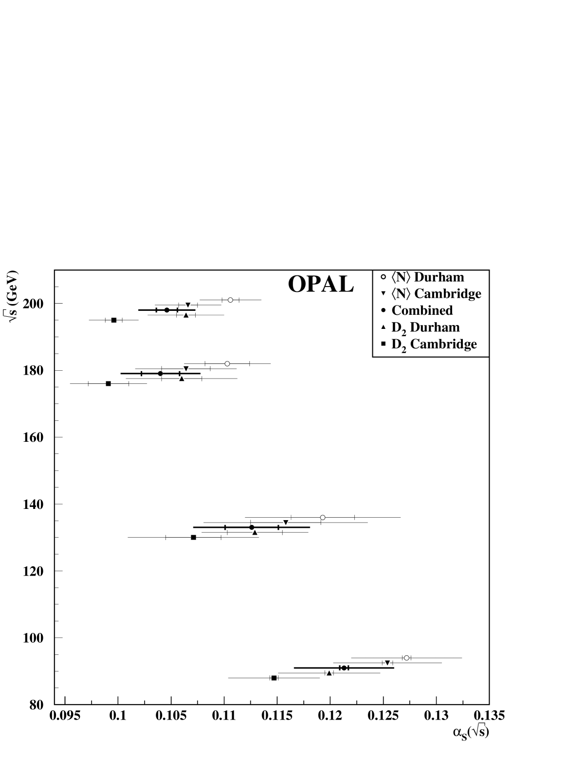
Figure 16: Comparison of combined $\alpha_{\rm{s}}$ values with those determined separately from the $D_{2}^{D}$, $D_{2}^{C}$, $\langle N\rangle^{C}$ and $\langle N\rangle^{D}$ distributions for each centre-of-mass energy dataset. Outer error bars indicate the size of the total errors while inner bars indicate the size of the statistical errors.

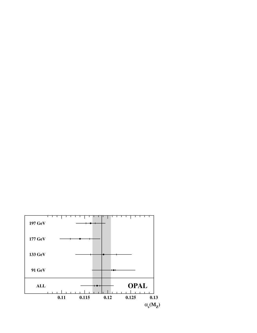
Figure 17: Comparison of the $\alpha_{\rm{s}}$ values after having been run back to the $\mathrm{Z}$ pole for each of the datasets. The point labelled by ’ALL’ represents the value determined from the weighted mean of the four combined $\alpha_{\rm{s}}$($M_{\mathrm{Z}}$) determinations. The shaded band corresponds to the one standard deviation range of the world average value of $\alpha_{\rm{s}}$($M_{\mathrm{Z}}$) [41]. The inner error bars represent the statistical errors while the outer error bars represent the total error.

The values of $\alpha_{\rm{s}}$ determined for each centre-of-mass energy are given in Table 9 along with the breakdown of the uncertainties, both statistical and systematic. A comparison of the combined $\alpha_{\rm{s}}$ values in Table 9 with those determined from the individual $D_{2}$ and $\langle N\rangle$ distributions is seen in Figure 16. Taking the combined $\alpha_{\rm{s}}$ values at each centre-of-mass energy as an input, the value of $\alpha_{\rm{s}}$ can be run back to the $\mathrm{Z}$ pole using an $\mathcal{O}(\mbox{$\alpha_{\rm{s}}^{3}$})$ prediction. These $\alpha_{\rm{s}}$($M_{\mathrm{Z}}$) values are also shown in Table 9 and plotted against the world average value of $\alpha_{\rm{s}}$($M_{\mathrm{Z}}$)=0.1187$\pm$0.0020 [41] in Fig 17. Using these values and taking into account proper statistical and systematic correlations, a weighted mean of $\alpha_{\rm{s}}$($M_{\mathrm{Z}}$)=$0.1177\pm 0.0006$(stat.)$\pm 0.0012$(expt.)$\pm 0.0010$(had.)$\pm 0.0032$(theo.) is determined. The four combined $\alpha_{\rm{s}}$ values are plotted in Figure 18 as a function of the centre-of-mass energy, compared to the $\mathcal{O}(\mbox{$\alpha_{\rm{s}}^{2}$})$ energy evolution of $\alpha_{\rm{s}}$ based on the determined value of $\alpha_{\rm{s}}$($M_{\mathrm{Z}}$).

8 Summary and Conclusion

Data from twelve LEP 1.5 and LEP 2 datasets, with centre-of-mass energies ranging from 130 GeV to 209 GeV, were combined into three higher statistics datasets. These datasets and one combining several $\mathrm{Z}$-calibration runs at 91 GeV were used to determine the $n$-jet fractions, the differential $n$-jet rates and the average jet rates for each of the energies. The different jet multiplicity distributions were compared to both PYTHIA and HERWIG Monte Carlo expectations.

Hadron-level $n$-jet fractions were determined using four jet-clustering algorithms, Cone, JADE, Durham and Cambridge. For the Cone algorithm, measurements of the fraction of events with $n\leq 2$, 3, $\geq$4 jets were presented as functions of $R$ and $\varepsilon$. In the case of JADE, Durham and Cambridge, measurements of the 2-, 3-, 4-, and 5-jet fractions were presented as functions of the jet resolution parameter, $y_{\rm{cut}}$. In all cases there was generally good agreement between the measured jet fractions and the Monte Carlo expectations.

Hadron-level determinations of the differential $n$-jet and average jet rates were performed for the Durham and Cambridge algorithms. The differential two-jet rate, $D_{2}$, and the average jet rate, $\langle N\rangle$ were used to determine the value of $\alpha_{\rm{s}}$($\sqrt{s}$) for each of the four combined energy points. The determinations were carried out by fitting the ln$R$ matching predictions, appropriately corrected to the hadron level, to the hadron level data distributions over an appropriate range of $y_{\rm{cut}}$, with $\alpha_{\rm{s}}$($\sqrt{s}$) as the variable parameter. The running of $\alpha_{\rm{s}}$($\sqrt{s}$) was demonstrated by comparing the four values of $\alpha_{\rm{s}}$ as determined from the combined datasets as a function of their centre-of-mass energies.

Using the measured values of $\alpha_{\rm{s}}$($\sqrt{s}$) a value of $\alpha_{\rm{s}}$($M_{\mathrm{Z}}$) was determined for each of the four datasets. A weighted mean taking account of correlations determined a final value of the strong coupling at $\sqrt{s}$ =$M_{\mathrm{Z}}$ of

$$\mbox{$\alpha_{\rm{s}}$}(M_{\mathrm{Z}})=0.1177\pm 0.0006(\mathrm{stat.})\pm 0.0012(\mathrm{expt.})\pm 0.0010(\mathrm{had.})\pm 0.0032(\mathrm{theo.})$$

where the error contains contributions from statistical, experimental, hadronization and theoretical uncertainties. The error on the determined value is slightly larger than that for the previous OPAL publication [6] which also used resummed predictions for $D_{2}$ and average jet rate distributions, but explored slightly different energy ranges, including 35 and 45 GeV, and all LEP energies up to only 189 GeV. There is good agreement between these four values of $\alpha_{\rm{s}}$($M_{\mathrm{Z}}$) measured in this analysis and previous determinations of $\alpha_{\rm{s}}$ summarized in [1] and with the world average value of 0.1187$\pm$0.0020 [41].

	Energy (GeV)			Integrated	Number of Events
Year	Nominal	Range	Mean	Luminosity	Data	JETSET/	HERWIG
				(pb-1)		PYTHIA
1996–2000	91	91.0–91.5	91.3	14.7	426194	459k	443k
1995, 1997	130	130.0–130.3	130.1	5.3	1628	50k	50k
1995, 1997	136	135.7–136.2	136.1	6.0	1504	50k	50k
1996	161	161.2–161.6	161.3	10.1	1369	100k	80k
1996	172	170.2–172.5	172.1	10.4	1285	100k	80k
1997	183	180.8–184.2	182.7	57.7	6027	100k	100k
1998	189	188.3–189.1	188.6	185.2	18559	500k	100k
1999	192	191.4–192.1	191.6	29.5	2866	200k	100k
1999	196	195.4–196.1	195.5	76.7	7076	200k	100k
1999, 2000	200	199.1–200.2	199.5	79.3	6676	200k	100k
1999, 2000	202	201.3–202.1	201.6	37.8	3225	200k	100k
2000	205	202.5–205.5	204.9	82.0	6721	200k	100k
2000	207	205.5–208.9	206.6	138.8	10987	375k	100k

Table 1: Integrated luminosity and the total number of preselected events for all samples. Included in this table are the Monte Carlo samples used to correct and make comparisons withthe data. The 91 GeV dataset corresponds to the data collected during the $\mathrm{Z}$-calibration runs.

Dataset		ISR Fit	Final
91 GeV	Data	395695	395695
130 GeV	Data	318	318
	MC Expected	368 $\pm$ 3	368 $\pm$ 3
	non-rad eff(%)	85.4 $\pm$ 1.4	85.4 $\pm$ 1.4
136 GeV	Data	312	312
	MC Expected	329 $\pm$ 3	329 $\pm$ 3
	non-rad eff(%)	85.5 $\pm$ 1.4	85.5 $\pm$ 1.4
161 GeV	Data	304	281
	MC Expected	299 $\pm$ 4	274 $\pm$ 3
	non-rad eff(%)	83.4 $\pm$ 1.0	80.0 $\pm$ 1.0
	4f bkg frac (%)	6.2 $\pm$ 1.7	2.1 $\pm$ 1.4
172 GeV	Data	280	218
	MC Expected	288 $\pm$ 7	232 $\pm$ 3
	non-rad eff(%)	83.3 $\pm$ 1.0	79.6 $\pm$ 1.0
	4f bkg frac (%)	19.7 $\pm$ 2.2	4.4 $\pm$ 1.7
183 GeV	Data	1456	1077
	MC Expected	1478 $\pm$ 22	1083 $\pm$ 11
	non-rad eff(%)	83.0 $\pm$ 1.0	79.0 $\pm$ 1.0
	4f bkg frac (%)	27.3 $\pm$ 1.2	5.5 $\pm$ 1.2
189 GeV	Data	4448	3086
	MC Expected	4497 $\pm$ 37	3130 $\pm$16
	non-rad eff(%)	83.0 $\pm$ 0.4	78.1 $\pm$ 0.4
	4f bkg frac (%)	30.0 $\pm$ 0.6	5.5 $\pm$ 0.6

Dataset		ISR Fit	Final
192 GeV	Data	717	514
	MC Expected	696$\pm$14	471$\pm$4
	non-rad eff(%)	82.8$\pm$0.7	77.4$\pm$0.7
	4f bkg frac (%)	31.3$\pm$1.5	5.3$\pm$1.2
196 GeV	Data	1732	1137
	MC Expected	1746$\pm$24	1162$\pm$9
	non-rad eff(%)	82.7$\pm$0.7	77.1$\pm$0.6
	4f bkg frac (%)	32.6$\pm$1.0	5.8$\pm$1.0
200 GeV	Data	1636	1090
	MC Expected	1717 $\pm$25	1130$\pm$10
	non-rad eff(%)	82.6$\pm$0.7	76.9$\pm$0.7
	4f bkg frac (%)	33.6$\pm$1.0	6.0$\pm$1.0
202 GeV	Data	806	519
	MC Expected	804$\pm$16	527$\pm$5
	non-rad eff(%)	85.4$\pm$0.7	76.9$\pm$0.7
	4f bkg frac (%)	34.1$\pm$1.4	6.2$\pm$1.2
205 GeV	Data	1687	1130
	MC Expected	1693$\pm$25	1089$\pm$9
	non-rad eff(%)	82.4$\pm$0.7	76.3$\pm$0.7
	4f bkg frac (%)	34.8$\pm$1.0	6.2$\pm$1.0
207 GeV	Data	2713	1717
	MC Expected	2807$\pm$32	1804$\pm$12
	non-rad eff(%)	82.7$\pm$0.5	76.5$\pm$0.5
	4f bkg frac (%)	34.7$\pm$0.8	6.2$\pm$0.6

Table 2: Effect of selection cuts (see text) on the number of observed events and the expectation from Monte Carlo simulations for the $\mathrm{q}\overline{\mathrm{q}}$ signal plus the four-fermion background. The quoted errors are purely statistical and do not reflect any experimental or hadronization systematics. The efficiency to select non-radiative $\mathrm{q}\overline{\mathrm{q}}$ events with $\sqrt{s}-\sqrt{s^{\prime}}<1$ GeV and the expected fraction of four-fermion background are also shown. The four-fermion background is negligible below 161 GeV.

Category	Error Source	Standard	Variation 1	Variation 2
	Track-Cluster Matching∗	MT objects	Tracks + Clusters
	Detector Correction∗	PYTHIA	HERWIG
	Containment ($|\cos\theta_{\rm{T}}|$)∗	$<0.9$	$<0.7$
(exp.)	qqqq ($\mathcal{L}$${}_{\mathrm{q}\overline{\mathrm{q}}\mathrm{q}\overline{\mathrm{q}}}$)	$<0.25$	$<0.1$	$<0.4$
	qql$\nu$($\mathcal{L}$${}_{\mathrm{q}\overline{\mathrm{q}}\ell\nu}$)	$<0.5$	$<0.75$	$<0.25$
	ISR Algorithm	Ref. [31]	Ref. [37]
	Backgrounds ($\sigma_{\rm{bkgd}}$)	1.0	+5%	$-$5%
(had.)	Hadronization∗	PYTHIA	HERWIG
(theo.)	Fit Range∗	min 6 bins	+2(1) bins	$-$2 bins
	Renorm. Scale Dep. ($x_{\mu}$)∗	1	0.5	2.0

Table 3: Summary of systematic variations applied to the datasets. The $\ast$ indicates which of the systematic variations were used for the 91 GeV dataset.

	91 GeV	133 GeV	177 GeV	197 GeV
$\alpha_{\rm{s}}$ ($\sqrt{s}$)	0.1147	0.1071	0.0991	0.0996
Fit Range ($-\log_{10}\mbox{$y_{\rm{cut}}$}$)	2.06–0.81	2.75–0.75	2.75–0.75	2.75–0.75
$\chi^{2}$ /dof	7.98/10	7.74/8	10.33/8	8.63/8
Experimental	$\pm$0.0017	$\pm$0.0032	$\pm$0.0019	$\pm$0.0009
Hadronization	$\pm$0.0026	$\pm$0.0007	$\pm$0.0005	$\pm$0.0005
Fit Range Variation	$\pm$0.0005	$\pm$0.0035	$\pm$0.0008	$\pm$0.0004
$x_{\mu}\ ^{x_{\mu}=2.0}{}_{x_{\mu}=0.5}$	${}^{+0.0030}_{-0.0010}$	${}^{+0.0030}_{-0.0014}$	${}^{+0.0023}_{-0.0011}$	${}^{+0.0020}_{-0.0010}$
$x_{L}\ ^{x_{L}=9/4}{}_{x_{L}=4/9}$	( ${}^{+0.0040}_{-0.0026}$)	( ${}^{+0.0033}_{-0.0022}$)	( ${}^{+0.0026}_{-0.0018}$)	( ${}^{+0.0025}_{-0.0019}$)
Theoretical	$\pm$0.0030	$\pm$0.0046	$\pm$0.0024	$\pm$0.0020
Total Stat.	$\pm$0.0004	$\pm$0.0026	$\pm$0.0019	$\pm$0.0008
Total Syst.	$\pm$0.0043	$\pm$0.0056	$\pm$0.0031	$\pm$0.0022
Total Error	$\pm$0.0043	$\pm$0.0062	$\pm$0.0037	$\pm$0.0024

Table 4: Determination of $\alpha_{\rm{s}}$ and the breakdown of statistical and systematic errors from the fit to the Cambridge differential two-jet rate distribution ($D_{2}^{\rm{C}}$) for all centre-of-mass energy values. The quality of the fit is characterized by the chi-square ($\chi^{2}$) and the number of degrees of freedom (dof). The theoretical error includes contributions from the fit range and $x_{\mu}$ variations and excludes the $x_{L}$ variation, which is used only for comparison.

	91 GeV	133 GeV	177 GeV	197 GeV
$\alpha_{\rm{s}}$ ($\sqrt{s}$)	0.1199	0.1129	0.1060	0.1064
Fit Range ($-\log_{10}\mbox{$y_{\rm{cut}}$}$)	1.81–0.68	2.75–0.75	2.75–0.75	2.50–0.75
$\chi^{2}$/dof	4.02/9	7.02/8	1.59/8	9.10/7
Experimental	$\pm$0.0025	$\pm$0.0026	$\pm$0.0013	$\pm$0.0007
Hadronization	$\pm$0.0017	$\pm$0.0005	$\pm$0.0005	$\pm$0.0007
Fit Range Variation	$\pm$0.0005	$\pm$0.0020	$\pm$0.0035	$\pm$0.0015
$x_{\mu}\ ^{x_{\mu}=2.0}{}_{x_{\mu}=0.5}$	${}^{+0.0037}_{-0.0013}$	${}^{+0.0028}_{-0.0020}$	${}^{+0.0031}_{-0.0017}$	${}^{+0.0030}_{-0.0014}$
$x_{L}\ ^{x_{L}=9/4}{}_{x_{L}=4/9}$	( ${}^{+0.0044}_{-0.0027}$)	( ${}^{+0.0028}_{-0.0026}$)	( ${}^{+0.0031}_{-0.0022}$)	( ${}^{+0.0032}_{-0.0020}$)
Theoretical	$\pm$0.0037	$\pm$0.0034	$\pm$0.0047	$\pm$0.0034
Total Stat.	$\pm$0.0004	$\pm$0.0026	$\pm$0.0019	$\pm$0.0009
Total Syst.	$\pm$0.0048	$\pm$0.0043	$\pm$0.0049	$\pm$0.0035
Total Error	$\pm$0.0048	$\pm$0.0050	$\pm$0.0052	$\pm$0.0037

Table 5: Determination of $\alpha_{\rm{s}}$ and the breakdown of statistical and systematic errors from the fit to the Durham differential two-jet rate distribution ($D_{2}^{\rm{D}}$) for all centre-of-mass energy values. The quality of the fit is characterized by the chi-square ($\chi^{2}$) and the number of degrees of freedom (dof). The theoretical error includes contributions from the fit range and $x_{\mu}$ variations and excludes the $x_{L}$ variation, which is used only for comparison.

	91 GeV	133 GeV	177 GeV	197 GeV
$\alpha_{\rm{s}}$ ($\sqrt{s}$)	0.1254	0.1158	0.1064	0.1066
Fit Range ($-\log_{10}\mbox{$y_{\rm{cut}}$}$)	2.56–0.56	2.75–0.50	2.75–0.50	2.75–0.50
$\chi^{2}$/dof	20.70/16	7.38/9	2.57/9	5.16/9
Experimental	$\pm$0.0013	$\pm$0.0040	$\pm$0.0030	$\pm$0.0015
Hadronization	$\pm$0.0033	$\pm$0.0034	$\pm$0.0018	$\pm$0.0017
Fit Range Variation	$\pm$0.0008	$\pm$0.0042	$\pm$0.0020	$\pm$0.0010
$x_{\mu}\ ^{x_{\mu}=2.0}{}_{x_{\mu}=0.5}$	${}^{+0.0036}_{-0.0001}$	${}^{+0.0021}_{-0.0001}$	${}^{+0.0016}_{-0.0001}$	${}^{+0.0016}_{-0.0001}$
Theoretical	$\pm$0.0037	$\pm$0.0047	$\pm$0.0026	$\pm$0.0019
Total Stat.	$\pm$0.0005	$\pm$0.0033	$\pm$0.0023	$\pm$0.0009
Total Syst.	$\pm$0.0051	$\pm$0.0070	$\pm$0.0042	$\pm$0.0030
Total Error	$\pm$0.0051	$\pm$0.0077	$\pm$0.0048	$\pm$0.0031

Table 6: Determination of $\alpha_{\rm{s}}$ and the breakdown of statistical and systematic errors from the fit to the Cambridge average jet rate distribution ($\langle N\rangle^{\rm{C}}$) for all centre-of-mass energy values. The quality of the fit is characterized by the chi-square ($\chi^{2}$) and the number of degrees of freedom (dof).

	91 GeV	133 GeV	177 GeV	197 GeV
$\alpha_{\rm{s}}$ ($\sqrt{s}$)	0.1272	0.1193	0.1103	0.1106
Fit Range ($-\log_{10}\mbox{$y_{\rm{cut}}$}$)	2.56–0.56	2.75–0.50	2.75–0.50	2.75–0.50
$\chi^{2}$/dof	7.90/16	4.73/9	0.81/9	4.14/9
Experimental	$\pm$0.0006	$\pm$0.0039	$\pm$0.0026	$\pm$0.0013
Hadronization	$\pm$0.0039	$\pm$0.0037	$\pm$0.0009	$\pm$0.0007
Fit Range Variation	$\pm$0.0003	$\pm$0.0029	$\pm$0.0003	$\pm$0.0008
$x_{\mu}\ ^{x_{\mu}=2.0}{}_{x_{\mu}=0.5}$	${}^{+0.0034}_{-0.0013}$	${}^{+0.0028}_{-0.0010}$	${}^{+0.0023}_{-0.0008}$	${}^{+0.0023}_{-0.0008}$
Theoretical	$\pm$0.0034	$\pm$0.0040	$\pm$0.0023	$\pm$0.0024
Total Stat.	$\pm$0.0004	$\pm$0.0030	$\pm$0.0021	$\pm$0.0008
Total Syst.	$\pm$0.0052	$\pm$0.0067	$\pm$0.0035	$\pm$0.0028
Total Error	$\pm$0.0052	$\pm$0.0073	$\pm$0.0041	$\pm$0.0029

Table 7: Determination of $\alpha_{\rm{s}}$ and the breakdown of statistical and systematic errors from the fit to the Durham average jet rate distribution ($\langle N\rangle^{\rm{D}}$) for all centre-of-mass energy values. The quality of the fit is characterized by the chi-square ($\chi^{2}$) and the number of degrees of freedom (dof).

91 GeV	$D_{2}^{C}$	$D_{2}^{D}$	$\langle N\rangle^{C}$	$\langle N\rangle^{D}$
$D_{2}^{C}$	100	85	53	46
$D_{2}^{D}$	85	100	56	47
$\langle N\rangle^{C}$	53	56	100	75
$\langle N\rangle^{D}$	46	47	75	100

133 GeV	$D_{2}^{C}$	$D_{2}^{D}$	$\langle N\rangle^{C}$	$\langle N\rangle^{D}$
$D_{2}^{C}$	100	83	70	64
$D_{2}^{D}$	83	100	64	63
$\langle N\rangle^{C}$	70	64	100	81
$\langle N\rangle^{D}$	64	63	81	100

177 GeV	$D_{2}^{C}$	$D_{2}^{D}$	$\langle N\rangle^{C}$	$\langle N\rangle^{D}$
$D_{2}^{C}$	100	84	73	66
$D_{2}^{D}$	84	100	71	72
$\langle N\rangle^{C}$	73	71	100	82
$\langle N\rangle^{D}$	66	72	82	100

197 GeV	$D_{2}^{C}$	$D_{2}^{D}$	$\langle N\rangle^{C}$	$\langle N\rangle^{D}$
$D_{2}^{C}$	100	90	77	68
$D_{2}^{D}$	90	100	72	73
$\langle N\rangle^{C}$	77	72	100	82
$\langle N\rangle^{D}$	68	73	82	100

Table 8: Statistical correlation matrix determined for the combination of $\alpha_{\rm{s}}$ measurements from the four different observables for each of the four different datasets. Each matrix element is presented as a percentage (%).

	Value for $\sqrt{s}$					Value at $M_{\mathrm{Z}}$
$\sqrt{s}$ (GeV)	$\alpha_{\rm{s}}$	$\sigma_{\rm{stat.}}$	$\sigma_{\rm{exp.}}$	$\sigma_{\rm{hadr.}}$	$\sigma_{\rm{theory}}$	$\alpha_{\rm{s}}$	$\sigma_{\rm{stat.}}$	$\sigma_{\rm{exp.}}$	$\sigma_{\rm{hadr.}}$	$\sigma_{\rm{theory}}$
$M_{\mathrm{Z}}$	0.1213	0.0004	0.0013	0.0029	0.0034	0.1213	0.0004	0.0013	0.0029	0.0034
133	0.1126	0.0025	0.0028	0.0007	0.0039	0.1191	0.0028	0.0031	0.0008	0.0044
177	0.1039	0.0018	0.0018	0.0001	0.0028	0.1140	0.0021	0.0021	0.0001	0.0033
197	0.1046	0.0008	0.0009	0.0002	0.0023	0.1163	0.0010	0.0012	0.0003	0.0029

Table 9: Values of $\alpha_{\rm{s}}$ determined from the weighted average of the individual $\alpha_{\rm{s}}$ results at each centre-of-mass energy, along with statistical and systematic errors. The value $\alpha_{\rm{s}}$ for the dataset when run back to the $\mathrm{Z}$ pole are given on the right half of the table with full statistical and systematic errors.

Figure 1: The $\sqrt{s}-\sqrt{s^{\prime}}$ distribution for the 189 GeV dataset. The vertical line indicates where the cut was applied. The expected non-radiative $\mathrm{q}\overline{\mathrm{q}}$ signal ($\sqrt{s}-\sqrt{s^{\prime}_{\rm{true}}}<1$ GeV) was determined from Monte Carlo and normalized to the luminosity of the measured sample. Vertical error bars indicate the size of statistical errors, while horizontal error bars correspond to the bin width.

Figure 2: Distributions of the four-quark likelihood $\mathcal{L}$${}_{\mathrm{q}\overline{\mathrm{q}}\mathrm{q}\overline{\mathrm{q}}}$ (top) and semi-leptonic likelihood $\mathcal{L}$${}_{\mathrm{q}\overline{\mathrm{q}}\ell\nu}$ (bottom) for the 189 GeV dataset. The expected contribution of the four-quark non-QCD background to the total sample is shown by the dotted line, and the expected semi-leptonic four-fermion background is represented by the dashed line. The vertical lines indicate the values of the parameters where the cuts were applied. The expected $\mathrm{q}\overline{\mathrm{q}}$ signal was determined from Monte Carlo and normalized to the luminosity of the measured sample. Vertical error bars indicate the size of statistical errors, while the horizontal bars correspond to the bin width.

Figure 3: The hadron level $n$-jet rates for the $R$ and $\varepsilon$ variants of the Cone algorithm for the data with $\sqrt{s}=91$ GeV (top) and $\sqrt{s}=133$ GeV (bottom). In all plots the JETSET/PYTHIA and HERWIG Monte Carlo expectations are represented by the curves. Outer error bars indicate total errors while the inner bars indicate statistical errors.

Figure 4: The hadron level $n$-jet rates for the $R$ and $\varepsilon$ variants of the Cone algorithm for the data with $\sqrt{s}=179$ GeV (top) and $\sqrt{s}=198$ GeV (bottom). In all plots the PYTHIA and HERWIG Monte Carlo expectations are represented by the curves. Outer error bars indicate total errors while the inner bars indicate statistical errors.

Figure 5: The hadron level $n$-jet rates for the JADE algorithm for the data with $\sqrt{s}=91$ GeV (top left), $\sqrt{s}=133$ GeV (top right), $\sqrt{s}=179$ GeV (bottom left) and $\sqrt{s}=198$ GeV (bottom right). In all plots the JETSET/PYTHIA and HERWIG Monte Carlo expectations are represented by the curves. Outer error bars indicate total errors while the inner bars indicate statistical errors.

Figure 6: The hadron level $n$-jet rates for the Durham and Cambridge algorithms for the data with $\sqrt{s}=91$ GeV (top) and $\sqrt{s}=133$ GeV (bottom). In all plots the JETSET/PYTHIA and HERWIG Monte Carlo expectations are represented by the curves. Outer error bars indicate total errors while the inner bars indicate statistical errors.

Figure 7: The hadron level $n$-jet rates for the Durham and Cambridge algorithms for the data with $\sqrt{s}=179$ GeV (top) and $\sqrt{s}=198$ GeV (bottom). In all plots the PYTHIA and HERWIG Monte Carlo expectations are represented by the curves. Outer error bars indicate total errors while the inner bars indicate statistical errors.

test

Figure 8: The differential 2-, 3- and 4-jet rates at the hadron level as a function of $y_{cut}$ for the Cambridge and Durham algorithms for data with $\sqrt{s}=91$ GeV (top) and for the LEP1.5 combined dataset at $\sqrt{s}=133$ GeV (bottom). PYTHIA and HERWIG Monte Carlo expectations are represented by the curves. The differential 3- and 4-jet rates have a negative slope in the region of large $y_{\rm{cut}}$ and therefore the negative values of $D_{3}$ and $D_{4}$ are plotted (the positive values are not seen on the curves). Note that $D_{3}$ and $D_{4}$ are scaled down by one and two orders of magnitude, respectively, for clarity. Error bars indicate total (statistical + systematic) errors.

test

Figure 9: The differential 2-, 3- and 4-jet rates at the hadron level as a function of $y_{cut}$ for the Cambridge and Durham algorithms for two combined LEP2 datasets with $\sqrt{s}=177$ GeV (top) and $\sqrt{s}=197$ GeV (bottom). PYTHIA and HERWIG Monte Carlo expectations are represented by the curves. The differential 3- and 4-jet rates have a negative slope in the region of large $y_{\rm{cut}}$ and therefore the negative values of $D_{3}$ and $D_{4}$ are plotted (the positive values are not seen on the curves). Note that $D_{3}$ and $D_{4}$ are scaled down by one and two orders of magnitude, respectively, for clarity. Error bars indicate total (statistical + systematic) errors.

Figure 10: The average jet rates at the hadron level as a function of $y_{cut}$ for the Cambridge algorithm for the all centre-of-mass energies. PYTHIA and HERWIG Monte Carlo expectations are represented by the curves. Error bars indicate total (statistical + systematic) errors.

Figure 11: The average jet rates at the hadron level as a function of $y_{cut}$ for the Durham algorithm for the all centre-of-mass energies. PYTHIA and HERWIG Monte Carlo expectations are represented by the curves. Error bars indicate total (statistical + systematic) errors.

Figure 12: Fits of the parton level $D_{2}$ distribution using the Cambridge algorithm as a function of $y_{\rm{cut}}$ to the ln $R$ prediction for the 91 GeV (top left), 133 GeV (top right), 179 GeV (bottom left) and 198 GeV (bottom right) datasets. The inset plots show the pull of each point from the line of best fit vs $\log_{10}\mbox{$y_{\rm{cut}}$}$. The two vertical lines delineate the fit range. Vertical error bars represent statistical errors only.

Figure 13: Fits of the parton level $D_{2}$ distribution using the Durham algorithm as a function of $y_{\rm{cut}}$ to the ln $R$ prediction for the 91 GeV (top left), 133 GeV (top right), 179 GeV (bottom left) and 198 GeV (bottom right) datasets. The inset plots show the pull of each point from the line of best fit vs $\log_{10}\mbox{$y_{\rm{cut}}$}$. The two vertical lines delineate the fit range. Vertical Error bars represent statistical errors only.

Figure 14: Fits of the parton level $\langle N\rangle$ distribution using the Cambridge algorithm as a function of $y_{\rm{cut}}$ to the ln $R$ prediction for the 91 GeV (top left), 133 GeV (top right), 179 GeV (bottom left) and 198 GeV (bottom right) datasets. Vertical error bars represent statistical errors only. Note: pulls are not shown as there are very large bin-to-bin correlations.

Figure 15: Fits of the parton level $\langle N\rangle$ distribution using the Durham algorithm as a function of $y_{\rm{cut}}$ to the ln $R$ prediction for the 91 GeV (top left), 130 GeV (top right), 189 GeV (bottom left) and 207 GeV (bottom right) datasets. Vertical error bars represent statistical errors only. Note: pulls are not shown as there are very large bin-to-bin correlations.

Figure 18: The running of $\alpha_{\rm{s}}$ as a function of centre-of-mass energy. The points correspond to the $\mathrm{Z}$-calibration dataset, the combined LEP1.5 data and the two LEP2 regions 161–183 and 189–209, respectively. The solid line corresponds to the expectation based on the weighted mean of the four combined $\alpha_{\rm{s}}$($M_{\mathrm{Z}}$) determinations, and the outer dashed line to the total (statistical + systematic) uncertainty.

References

- [1] S. Bethke, Nucl. Phys. Proc. Suppl. 121 (2003) 74.
- [2] OPAL Collaboration, P. D. Acton et al., Z. Phys. C59 (1993) 1.
- [3] OPAL Collaboration, G. Alexander et al., Z. Phys. C72 (1996) 191.
- [4] OPAL Collaboration, K. Ackerstaff et al., Z. Phys. C75 (1997) 193.
- [5] OPAL Collaboration, G. Abbiendi et al., Eur. Phys. J. C16 (2000) 185.
- [6] JADE and OPAL Collaborations, P. Pfeifenschneider et al., Eur. Phys. J. C17 (2000) 19.
- [7] OPAL Collaboration, G. Abbiendi et al., Eur. Phys. J. C40 (2005) 287.
- [8] OPAL Collaboration, K. Ahmet et al., Nucl. Instrum. Meth. A305 (1991) 275.
- [9] OPAL Collaboration, G. Abbiendi et al., Eur. Phys. J. C14 (2000) 373.
- [10] OPAL Collaboration, M. Arignon et al., Nucl. Instrum. Meth. A313 (1992) 103.
- [11] OPAL Collaboration, J. T. M. Baines et al., Nucl. Instrum. Meth. A325 (1993) 271.
- [12] OPAL Collaboration, J. Allison et al., Nucl. Instrum. Meth. A317 (1992) 47.
- [13] T. Sjöstrand et al., Comput. Phys. Commun. 135 (2001) 238.
- [14] T. Sjöstrand, Comput. Phys. Commun. 82 (1994) 74.
- [15] G. Corcella et al., JHEP 01 (2001) 010.
- [16] OPAL Collaboration, G. Alexander et al., Z. Phys. C69 (1996) 534.
- [17] OPAL Collaboration, G. Abbiendi et al., Eur. Phys. J. C35 (2004) 293.
- [18] S. Jadach, B. Ward, and Z. Wa̧s, Comput. Phys. Commun. 130 (2000) 260.
- [19] M. Skrzypek, S. Jadach, W. Placzek, and Z. Wa̧s, Comput. Phys. Commun. 94 (1996) 216.
- [20] J. Fujimoto et al., Comput. Phys. Commun. 100 (1997) 128.
- [21] ALEPH, DELPHI, L3, OPAL and SLD Collaborations, A combination of preliminary electroweak measurements and constraints on the Standard Model, 2003, hep-ex/0312023.
- [22] S. Catani, Y. Dokshitzer, M. Olsson, G. Turnock, and B. Webber, Phys. Lett. B269 (1991) 432.
- [23] Y. L. Dokshitzer, G. D. Leder, S. Moretti, and B. R. Webber, JHEP 08 (1997) 001.
- [24] JADE Collaboration, W. Bartel et al., Z. Phys. C33 (1986) 23.
- [25] F. Abe et al., Phys. Lett. D45 (1992) 1448.
- [26] R. K. Ellis, D. A. Ross, and A. E. Terrano, Nucl. Phys. B178 (1981) 421.
- [27] S. Catani, L. Trentadue, G. Turnock, and B. Webber, Nucl. Phys. B407 (1992) 3.
- [28] A. Banfi, G. P. Salam, and G. Zanderighi, JHEP 01 (2002) 018.
- [29] G. Dissertori and M. Schmelling, Phys. Lett. B361 (1995) 167.
- [30] OPAL Collaboration, P. D. Acton et al., Z. Phys. C59 (1993) 1.
- [31] OPAL Collaboration, K. Ackerstaff et al., Eur. Phys. J. C2 (1998) 441.
- [32] OPAL Collaboration, G. Alexander et al., Z. Phys. C52 (1991) 175.
- [33] S. Brandt, C. Peyrou, R. Sosnowski, and A. Wroblewski, Phys. Lett. 12 (1964) 57.
- [34] OPAL Collaboration Collaboration, K. Ackerstaff et al., Phys. Lett. B391 (1997) 221.
- [35] OPAL Collaboration, G. Abbiendi et al., Eur. Phys. J. C16 (2000) 185.
- [36] OPAL Collaboration, G. Abbiendi et al., Phys. Lett. B493 (2000) 249.
- [37] OPAL Collaboration, K. Ackerstaff et al., Z. Phys. C75 (1997) 193.
- [38] M. Dasgupta and G. P. Salam, JHEP 08 (2002) 032.
- [39] R. W. L. Jones, M. Ford, G. P. Salam, H. Stenzel, and D. Wicke, JHEP 12 (2003) 007.
- [40] L. Lyons, D. Gibaut, and P. Clifford, Nucl. Instrum. Meth. A270 (1988) 110.
- [41] S. Eidelman et al., Phys. Lett. B592 (2004) 1.