Time-Dependent $CP$ Asymmetries in $b\to s\overline{q}q$ Transitions and ${\sin 2\phi_{1}}$ in ${B^{0}}\to{J/\psi}{K^{0}}$ Decays with 386 Million $B\overline{B}$ Pairs

Abstract

We present measurements of time-dependent $CP$ asymmetries in ${B^{0}}\to$ $\phi(1020){K^{0}}$, $\eta^{\prime}{K^{0}}$, ${K_{S}^{0}}{K_{S}^{0}}{K_{S}^{0}}$, ${K_{S}^{0}}{\pi^{0}}$, ${f_{0}}(980){K_{S}^{0}}$, $\omega(782){K_{S}^{0}}$ and ${K^{+}}{K^{-}}{K_{S}^{0}}$ decays based on a sample of $386\times 10^{6}$ $B{\overline{B}}$ pairs collected at the ${\Upsilon(4S)}$ resonance with the Belle detector at the KEKB energy-asymmetric $e^{+}e^{-}$ collider. These decays are dominated by the $b\to s$ gluonic penguin transition and are sensitive to new $CP$-violating phases from physics beyond the standard model. One neutral $B$ meson is fully reconstructed in one of the specified decay channels, and the flavor of the accompanying $B$ meson is identified from its decay products. $CP$-violation parameters ${\sin 2\phi_{1}^{\rm eff}}$ and ${\cal A}_{f}$ for each of the decay modes are obtained from the asymmetries in the distributions of the proper-time intervals between the two $B$ decays. We also perform an improved measurement of $CP$ asymmetries in ${B^{0}}\to{J/\psi}{K^{0}}$ decays using the same data sample. The same analysis procedure mentioned above yields ${\sin 2\phi_{1}}=+0.652\pm 0.039\mbox{(stat)}\pm 0.020\mbox{(syst)}$, which serves as a reference point for the standard model, and ${\cal A}_{f}=+0.010\pm 0.026\mbox{(stat)}\pm 0.036\mbox{(syst)}$.

I Introduction

The flavor-changing $b\to s$ transition proceeds through loop penguin diagrams. Such loop diagrams play an important role in testing the standard model (SM) and new physics because particles beyond the SM can contribute via additional loop diagrams. $CP$ violation in the $b\to s$ transition is especially sensitive to physics at a very high-energy scale Akeroyd:2004mj . Theoretical studies indicate that large deviations from the SM expectations are allowed for time-dependent $CP$ asymmetries in ${B^{0}}$ meson decays bib:lucy . Experimental investigations have recently been launched at the two $B$ factories, each of which has produced more than $10^{8}$ $B{\overline{B}}$ pairs. The first measurement of the $CP$-violating asymmetry in ${B^{0}}\to\phi{K_{S}^{0}}$ decays footnote:CC , which are dominated by the $b\to s\overline{s}s$ transition, by the Belle collaboration indicated deviation from the SM expectation Abe:2003yt . Measurements with a larger data sample are required to confirm this difference. It is also essential to examine additional modes that are sensitive to the same $b\to s$ penguin amplitude. In this spirit, experimental results based on a sample of $275\times 10^{6}$ $B{\overline{B}}$ pairs using decay modes ${B^{0}}\to$ $\phi{K^{0}}$, $\eta^{\prime}{K_{S}^{0}}$, ${K_{S}^{0}}{K_{S}^{0}}{K_{S}^{0}}$, ${K_{S}^{0}}{\pi^{0}}$, ${f_{0}}{K_{S}^{0}}$, $\omega{K_{S}^{0}}$, and ${K^{+}}{K^{-}}{K_{S}^{0}}$ footnote:mesons have already been reported Chen:2005dr ; Sumisawa:2005fz . The combined result differs from the SM expectation by 2.4 standard deviations. Since measurements by the BaBar collaboration also yield a similar deviation bib:HFAG ; bib:BaBar_sss , the present world average differs from the SM expectation by 3.7 standard deviations.

In the SM, $CP$ violation arises from a single irreducible phase, the Kobayashi-Maskawa (KM) phase Kobayashi:1973fv , in the weak-interaction quark-mixing matrix. In particular, the SM predicts $CP$ asymmetries in the time-dependent rates for ${B^{0}}$ and ${\overline{B}{}^{0}}$ decays to a common $CP$ eigenstate $f_{CP}$ bib:sanda . In the decay chain $\Upsilon(4S)\to{B^{0}}{\overline{B}{}^{0}}\to f_{CP}f_{\rm tag}$, where one of the $B$ mesons decays at time $t_{CP}$ to a final state $f_{CP}$ and the other decays at time $t_{\rm tag}$ to a final state $f_{\rm tag}$ that distinguishes between $B^{0}$ and ${\overline{B}{}^{0}}$, the decay rate has a time dependence given by

$${\cal P}(\Delta{t})=\frac{e^{-|\Delta{t}|/{{\tau_{B^{0}}}}}}{4{{\tau_{B^{0}}}}}\biggl{\{}1+q\cdot\Bigl{[}{\cal S}_{f}\sin(\Delta m_{d}\Delta{t})+{\cal A}_{f}\cos(\Delta m_{d}\Delta{t})\Bigr{]}\biggr{\}}.$$ (1)

Here ${\cal S}_{f}$ and ${\cal A}_{f}$ are $CP$-violation parameters, ${\tau_{B^{0}}}$ is the $B^{0}$ lifetime, $\Delta m_{d}$ is the mass difference between the two $B^{0}$ mass eigenstates, $\Delta{t}$ = $t_{CP}$ $-$ $t_{\rm tag}$, and the $b$-flavor charge $q$ = +1 ($-1$) when the tagging $B$ meson is a $B^{0}$ (${\overline{B}{}^{0}}$). To a good approximation, the SM predicts ${\cal S}_{f}=-\xi_{f}{\sin 2\phi_{1}}$, where $\xi_{f}=+1(-1)$ corresponds to $CP$-even (-odd) final states, and ${\cal A}_{f}=0$ for both $b\to c\overline{c}s$ and $b\to s\overline{q}q$ transitions. Therefore, a comparison of $CP$-violation parameters between $b\to s\overline{q}q$ and $b\to c\overline{c}s$ decays is an important test of the SM.

Recent theoretical studies bib:b2s_SM_uncertainties find that ${B^{0}}\to\phi{K^{0}}$, ${\eta^{\prime}}{K^{0}}$ and ${K_{S}^{0}}{K_{S}^{0}}{K_{S}^{0}}$ have the smallest hadronic uncertainties among the modes listed above. The effective ${\sin 2\phi_{1}}$ values, ${\sin 2\phi_{1}^{\rm eff}}$, obtained from these decays are expected to agree with ${\sin 2\phi_{1}}$ from the ${B^{0}}\to{J/\psi}{K^{0}}$ decay within 0.04. Larger deviations would indicate a new $CP$-violating phase beyond the SM. The other modes may be affected by a larger amount by the $b\to u$ transition that has a weak phase $\phi_{3}$. Correspondingly, the SM predictions for the ${\sin 2\phi_{1}^{\rm eff}}$ values of these modes suffer larger uncertainties.

Belle’s previous measurements of $CP$ violation in ${B^{0}}\to$ $\phi{K_{S}^{0}}$, $\phi{K_{L}^{0}}$, $\eta^{\prime}{K_{S}^{0}}$, ${K_{S}^{0}}{K_{S}^{0}}{K_{S}^{0}}$, ${K_{S}^{0}}{\pi^{0}}$, ${f_{0}}{K_{S}^{0}}$, $\omega{K_{S}^{0}}$ and ${K^{+}}{K^{-}}{K_{S}^{0}}$ decays were based on a $253$ fb^-1 data sample containing $275\times 10^{6}$ $B{\overline{B}}$ pairs. In this report, we describe improved measurements for these decays incorporating an additional $104$ fb^-1 data sample that contains $111\times 10^{6}$ $B{\overline{B}}$ pairs for a total of $386\times 10^{6}$ $B{\overline{B}}$ pairs. We also measure $CP$ asymmetries for ${B^{0}}\to\eta^{\prime}{K_{L}^{0}}$ and $\eta^{\prime}{K_{S}^{0}}$ followed by ${K_{S}^{0}}\to{\pi^{0}}{\pi^{0}}$, which were not included in the previous analysis.

Recent measurements of time-dependent $CP$ asymmetries in decay modes governed by the $b\to c\overline{c}s$ transition by Belle bib:CP1_Belle ; bib:BELLE-CONF-0436 and BaBar bib:CP1_BaBar have determined ${\sin 2\phi_{1}}=+0.726\pm 0.037$ bib:HFAG , where ${B^{0}}\to{J/\psi}{K_{S}^{0}}$, ${J/\psi}{K_{L}^{0}}$, $\psi(2S){K_{S}^{0}}$, $\chi_{c1}{K_{S}^{0}}$ and $\eta_{c}{K_{S}^{0}}$ decays are used. In this report, we describe improved measurements of $CP$-violation parameters ${\cal S}_{f}$ and ${\cal A}_{f}$ in ${B^{0}}\to{J/\psi}{K_{S}^{0}}$ and ${J/\psi}{K_{L}^{0}}$ decays, which are the modes with the largest statistics and with the smallest theoretical uncertainties Boos:2004xp ; Atwood:2003tg , as a firm reference point for the SM.

Among the $b\to s$ modes listed above, all of the two-body final states are $CP$ eigenstates with a $CP$ eigenvalue $\xi_{f}=-1$ ($\phi{K_{S}^{0}}$, $\eta^{\prime}{K_{S}^{0}}$, ${K_{S}^{0}}{\pi^{0}}$ and $\omega{K_{S}^{0}}$) or $\xi_{f}=+1$ ($\phi{K_{L}^{0}}$, $\eta^{\prime}{K_{L}^{0}}$ and ${f_{0}}{K_{S}^{0}}$). While the three body state ${K_{S}^{0}}{K_{S}^{0}}{K_{S}^{0}}$ is a $CP$ eigenstate with $\xi_{f}=+1$ Gershon:2004tk , the ${K^{+}}{K^{-}}{K_{S}^{0}}$ state is in general a mixture of both $CP$-even and -odd final states. Excluding ${K^{+}}{K^{-}}$ pairs that are consistent with a $\phi\to{K^{+}}{K^{-}}$ decay from the ${B^{0}}\to K^{+}K^{-}{K_{S}^{0}}$ sample, we find that the ${K^{+}}{K^{-}}{K_{S}^{0}}$ state is primarily $CP$-even; a measurement of the $CP$-even fraction $f_{+}$ using the isospin relation Garmash:2003er with a $357$ fb^-1 data sample gives $f_{+}=0.93\pm 0.09\mbox{(stat)}\pm 0.05\mbox{(syst)}$. The SM expectation for this mode is ${\cal S}_{f}=-(2f_{+}-1)\sin 2\phi_{1}$. In this report, we define $\xi_{f}\equiv 2f_{+}-1=+0.86\pm 0.18\mbox{(stat)}\pm 0.09\mbox{(syst)}$ for the ${B^{0}}\to{K^{+}}{K^{-}}{K_{S}^{0}}$ decay, and measure ${\sin 2\phi_{1}^{\rm eff}}\equiv-\xi_{f}^{-1}{\cal S}_{f}$.

The decays ${B^{0}}\to\phi{K_{S}^{0}}$ and $\phi{K_{L}^{0}}$ are combined in this analysis by redefining ${\cal S}_{f}$ as $-\xi_{f}{\cal S}_{f}$ to take the opposite $CP$ eigenvalues into account, and are collectively called “${B^{0}}\to\phi{K^{0}}$”. Likewise, $CP$ asymmetries for “${B^{0}}\to\eta^{\prime}{K^{0}}$” or “${B^{0}}\to{J/\psi}{K^{0}}$” are obtained by combining the decays ${B^{0}}\to\eta^{\prime}{K_{S}^{0}}$ and $\eta^{\prime}{K_{L}^{0}}$, or ${B^{0}}\to{J/\psi}{K_{S}^{0}}$ and ${J/\psi}{K_{L}^{0}}$.

At the KEKB energy-asymmetric $e^{+}e^{-}$ (3.5 on 8.0 GeV) collider bib:KEKB , the $\Upsilon(4S)$ is produced with a Lorentz boost of $\beta\gamma=0.425$ nearly along the electron beamline ($z$). Since the $B^{0}$ and ${\overline{B}{}^{0}}$ mesons are approximately at rest in the $\Upsilon(4S)$ center-of-mass system (cms), $\Delta t$ can be determined from the displacement in $z$ between the $f_{CP}$ and $f_{\rm tag}$ decay vertices: $\Delta t\simeq(z_{CP}-z_{\rm tag})/(\beta\gamma c)\equiv\Delta z/(\beta\gamma c)$.

The Belle detector is a large-solid-angle magnetic spectrometer that consists of a silicon vertex detector (SVD), a 50-layer central drift chamber (CDC), an array of aerogel threshold Cherenkov counters (ACC), a barrel-like arrangement of time-of-flight scintillation counters (TOF), and an electromagnetic calorimeter comprised of CsI(Tl) crystals (ECL) located inside a superconducting solenoid coil that provides a 1.5 T magnetic field. An iron flux-return located outside of the coil is instrumented to detect $K_{L}^{0}$ mesons and to identify muons (KLM). The detector is described in detail elsewhere Belle . Two inner detector configurations were used. A 2.0 cm radius beampipe and a 3-layer silicon vertex detector (SVD-I) were used for the first $140$ fb^-1 data sample (DS-I) that contains $152\times 10^{6}$ $B{\overline{B}}$ pairs, while a 1.5 cm radius beampipe, a 4-layer silicon detector (SVD-II) Ushiroda and a small-cell inner drift chamber were used for the rest, a $217$ fb^-1 data sample (DS-II) that contains $234\times 10^{6}$ $B{\overline{B}}$ pairs.

II Event Selection, Flavor Tagging and Vertex Reconstruction

II.1 Overview

We reconstruct the following ${B^{0}}$ decay modes to measure $CP$ asymmetries: ${B^{0}}\to$ $\phi{K_{S}^{0}}$, $\phi{K_{L}^{0}}$, $\eta^{\prime}{K_{S}^{0}}$, $\eta^{\prime}{K_{L}^{0}}$, ${K_{S}^{0}}{K_{S}^{0}}{K_{S}^{0}}$, ${K_{S}^{0}}{\pi^{0}}$, ${f_{0}}{K_{S}^{0}}$, $\omega{K_{S}^{0}}$ and ${K^{+}}{K^{-}}{K_{S}^{0}}$. We exclude $K^{+}K^{-}$ pairs that are consistent with a $\phi\to K^{+}K^{-}$ decay from the ${B^{0}}\to K^{+}K^{-}{K_{S}^{0}}$ sample. The intermediate meson states are reconstructed from the following decays: ${\pi^{0}}\to\gamma\gamma$, ${K_{S}^{0}}\to{\pi^{+}}{\pi^{-}}$, $\eta\to\gamma\gamma$, ${\rho^{0}}\to{\pi^{+}}{\pi^{-}}$, $\omega\to{\pi^{+}}{\pi^{-}}{\pi^{0}}$, $\eta^{\prime}\to{\rho^{0}}\gamma$ or $\eta{\pi^{+}}{\pi^{-}}$, ${f_{0}}\to{\pi^{+}}{\pi^{-}}$, and $\phi\to K^{+}K^{-}$. In addition, ${K_{S}^{0}}\to{\pi^{0}}{\pi^{0}}$ decays are used for ${B^{0}}\to\phi{K_{S}^{0}}$ and $\eta^{\prime}{K_{S}^{0}}$ decays, and $\eta\to{\pi^{+}}{\pi^{-}}{\pi^{0}}$ for the case ${B^{0}}\to\eta^{\prime}{K_{S}^{0}}$ (${K_{S}^{0}}\to{\pi^{+}}{\pi^{-}}$).

II.2 ${B^{0}}\to\phi{K_{S}^{0}}$ and ${K^{+}}{K^{-}}{K_{S}^{0}}$

Charged tracks reconstructed with the CDC for kaon and pion candidates, except for tracks from ${K_{S}^{0}}\to{\pi^{+}}{\pi^{-}}$ decays, are required to originate from the interaction point (IP). We distinguish charged kaons from pions based on a kaon (pion) likelihood $\mathcal{L}_{K(\pi)}$ derived from the TOF, ACC and $dE/dx$ measurements in the CDC.

Pairs of oppositely charged tracks that have an invariant mass within 0.015 GeV/$c^{2}$ of the nominal ${K_{S}^{0}}$ mass are used to reconstruct ${K_{S}^{0}}\to{\pi^{+}}{\pi^{-}}$ decays. The distance of closest approach of the candidate charged tracks to the IP in the plane perpendicular to the $z$ axis is required to be larger than 0.02 cm for high momentum ($>1.5$ GeV/$c$) ${K_{S}^{0}}$ candidates and larger than 0.03 cm for those with momentum less than 1.5 GeV/$c$. The ${\pi^{+}}{\pi^{-}}$ vertex is required to be displaced from the IP by a minimum transverse distance of 0.22 cm for high-momentum candidates and 0.08 cm for the remaining candidates. The mismatch in the $z$ direction at the ${K_{S}^{0}}$ vertex point for the ${\pi^{+}}{\pi^{-}}$ tracks must be less than 2.4 cm for high-momentum candidates and less than 1.8 cm for the remaining candidates. The direction of the pion pair momentum must also agree with the direction of the vertex point from the IP to within 0.03 rad for high-momentum candidates, and to within 0.1 rad for the remaining candidates. The resolution of the reconstructed ${K_{S}^{0}}$ mass is 0.003 GeV$/c^{2}$.

Photons are identified as isolated ECL clusters that are not matched to any charged track. To select ${K_{S}^{0}}\to{\pi^{0}}{\pi^{0}}$ decays, we reconstruct ${\pi^{0}}$ candidates from pairs of photons with $E_{\gamma}>0.05$ GeV, where $E_{\gamma}$ is the photon energy measured with the ECL. Photon pairs with an invariant mass between 0.08 and 0.15 GeV$/c^{2}$ and a momentum above 0.1 GeV/$c$ are used as ${\pi^{0}}$ candidates. Initially, the ${\pi^{0}}$ decay vertex is assumed to be the IP. An asymmetric mass window is used to take into account the lower tail of the mass distribution due to the distance between the IP and the true ${\pi^{0}}$ vertex. Candidate ${K_{S}^{0}}\to{\pi^{0}}{\pi^{0}}$ decays are required to have an invariant mass between 0.47 GeV/$c^{2}$ and 0.52 GeV/$c^{2}$, where we perform a fit with constraints on the ${K_{S}^{0}}$ vertex and the ${\pi^{0}}$ masses to improve the ${\pi^{0}}{\pi^{0}}$ invariant mass resolution. We also require that the distance between the IP and the reconstructed ${K_{S}^{0}}$ decay vertex be larger than $-10$ cm, where the positive direction is defined by the ${K_{S}^{0}}$ momentum.

Candidate $\phi\to{K^{+}}{K^{-}}$ decays are required to have an invariant mass that is within 0.01 GeV/$c^{2}$ of the nominal $\phi$ meson mass. Since the $\phi$ meson selection is effective in reducing background events, we impose only minimal kaon-identification requirements; ${\cal R}_{K/\pi}\equiv\mathcal{L}_{K}/(\mathcal{L}_{K}+\mathcal{L}_{\pi})>0.1$ is required, where the kaon likelihood ratio $\mathcal{R}_{K/\pi}$ has values between 0 (likely to be a pion) and 1 (likely to be a kaon). We use a more stringent kaon-identification requirement, ${\cal R}_{K/\pi}>0.6$, to select non-resonant ${K^{+}}{K^{-}}$ candidates for the decay ${B^{0}}\to{K^{+}}{K^{-}}{K_{S}^{0}}$. We exclude ${K^{+}}{K^{-}}$ pairs with an invariant mass within 0.015 GeV/$c^{2}$ of the nominal $\phi$ meson mass to reduce the $\phi$ contribution to a negligible level. To remove $\chi_{c0}\to K^{+}K^{-}$, $J/\psi\to K^{+}K^{-}$ and $D^{0}\to K^{+}K^{-}$ decays, $K^{+}K^{-}$ pairs with an invariant mass within 0.015 GeV$/c^{2}$ of the nominal masses of $\chi_{c0}$ and $J/\psi$ or within 0.01 GeV$/c^{2}$ of the nominal $D^{0}$ mass are rejected. $D^{+}\to{K_{S}^{0}}K^{+}$ decays are also removed by rejecting ${K_{S}^{0}}K^{+}$ pairs with an invariant mass within 0.01 GeV$/c^{2}$ of the nominal $D^{+}$ mass.

For reconstructed $B\to f_{CP}$ candidates, we identify $B$ meson decays using the energy difference ${\Delta E}\equiv E_{B}^{\rm cms}-E_{\rm beam}^{\rm cms}$ and the beam-energy constrained mass ${M_{\rm bc}}\equiv\sqrt{(E_{\rm beam}^{\rm cms})^{2}-(p_{B}^{\rm cms})^{2}}$, where $E_{\rm beam}^{\rm cms}$ is the beam energy in the cms, and $E_{B}^{\rm cms}$ and $p_{B}^{\rm cms}$ are the cms energy and momentum of the reconstructed $B$ candidate, respectively. The resolution of ${M_{\rm bc}}$ is about 0.003 GeV$/c^{2}$. Because of the smallness of $p_{B}^{\rm cms}$, the ${M_{\rm bc}}$ resolution is dominated by the beam-energy spread, which is common to all decay modes. The resolution in ${\Delta E}$ depends on the reconstructed decay mode. The ${\Delta E}$ resolution is 0.013 GeV for $\phi{K_{S}^{0}}~{}({K_{S}^{0}}\to{\pi^{+}}{\pi^{-}})$ and ${K^{+}}{K^{-}}{K_{S}^{0}}$. The ${\Delta E}$ distribution for $\phi{K_{S}^{0}}~{}({K_{S}^{0}}\to{\pi^{0}}{\pi^{0}})$ has a tail toward lower ${\Delta E}$ due to $\gamma$ energy leakage in the ECL. The typical ${\Delta E}$ resolution for $\phi{K_{S}^{0}}~{}({K_{S}^{0}}\to{\pi^{0}}{\pi^{0}})$ is 0.058 GeV for the main component and the typical width of the tail component is about 0.14 GeV. The $B$ meson signal region is defined as $|{\Delta E}|<0.06$ GeV for ${B^{0}}\to\phi{K_{S}^{0}}~{}({K_{S}^{0}}\to{\pi^{+}}{\pi^{-}})$, $-0.15~{}{\rm GeV}<{\Delta E}<0.1$ GeV for ${B^{0}}\to\phi{K_{S}^{0}}~{}({K_{S}^{0}}\to{\pi^{0}}{\pi^{0}})$, $|{\Delta E}|<0.04$ GeV for ${B^{0}}\to K^{+}K^{-}{K_{S}^{0}}$, and $5.27~{}{\rm GeV}/c^{2}<{M_{\rm bc}}<5.29~{}{\rm GeV}/c^{2}$ for all decays.

The dominant background to the ${B^{0}}\to\phi{K_{S}^{0}}$ and ${K^{+}}{K^{-}}{K_{S}^{0}}$ decays comes from $e^{+}e^{-}\rightarrow u\overline{u},~{}d\overline{d},~{}s\overline{s}$, or $c\overline{c}$ continuum events. Since these tend to be jet-like, while the signal events tend to be spherical, we use a set of variables that characterize the event topology to distinguish between the two. We combine ${S_{\perp}}$, $\theta_{T}$ and modified Fox-Wolfram moments Abe:2001nq into a Fisher discriminant ${\cal F}$, where ${S_{\perp}}$ is the scalar sum of the transverse momenta of particles other than the reconstructed $B$ candidate outside a $45^{\circ}$ cone around the candidate $\phi$ meson direction (the thrust axis of the $B$ candidate for ${K^{+}}{K^{-}}{K_{S}^{0}}$ decays) divided by the scalar sum of their total momenta, and $\theta_{T}$ is the angle between the thrust axis of the $B$ candidate and that of the other particles in the cms. We also use the angle of the reconstructed $B$ candidate with respect to the beam direction in the cms ($\theta_{B}$). We combine ${\cal F}$ and $\cos\theta_{B}$ into a signal [background] likelihood variable, which is defined as ${\cal L}_{\rm sig[bkg]}\equiv{\cal L}_{\rm sig[bkg]}({\cal F})\times{\cal L}_{\rm sig[bkg]}(\cos\theta_{B})$. We impose requirements on the likelihood ratio ${\cal R}_{\rm s/b}\equiv{\cal L}_{\rm sig}/({\cal L}_{\rm sig}+{\cal L}_{\rm bkg})$ to maximize the figure-of-merit (FoM) defined as ${N_{\rm sig}^{\rm MC}}/\sqrt{{N_{\rm sig}^{\rm MC}}+{N_{\rm bkg}}}$, where ${N_{\rm sig}^{\rm MC}}$ (${N_{\rm bkg}}$) represents the expected number of signal (background) events in the signal region. We estimate ${N_{\rm sig}^{\rm MC}}$ using Monte Carlo (MC) events, while ${N_{\rm bkg}}$ is determined from events outside the signal region.

We define two ${\cal R}_{\rm s/b}$ regions for the decay ${B^{0}}\to\phi{K_{S}^{0}}~{}({K_{S}^{0}}\to{\pi^{+}}{\pi^{-}})$. We require ${\cal R}_{\rm s/b}\geq 0.65$ for the high-${\cal R}_{\rm s/b}$ region. The requirement for the low-${\cal R}_{\rm s/b}$ region depends on the flavor-tagging quality, $r$, which is described in Sec. II.11. The threshold values range from 0.1 (used for $r>0.875$) to 0.35 (used for $r<0.25$). For the ${B^{0}}\to\phi{K_{S}^{0}}~{}({K_{S}^{0}}\to{\pi^{0}}{\pi^{0}})$ candidates, the ${\cal R}_{\rm s/b}$ threshold values depend on $r$ and range from 0.4 to 0.75, which are more stringent than those for the ${K_{S}^{0}}\to{\pi^{+}}{\pi^{-}}$ case. For the ${B^{0}}\to{K^{+}}{K^{-}}{K_{S}^{0}}$ candidates, we require $|\cos\theta_{T}|<0.9$ prior to the ${\cal R}_{\rm s/b}$ requirement. The ${\cal R}_{\rm s/b}$ threshold values range from 0.25 to 0.65. The ${\cal R}_{\rm s/b}$ requirement reduces the continuum background by 65% for ${B^{0}}\to\phi{K_{S}^{0}}~{}({K_{S}^{0}}\to{\pi^{+}}{\pi^{-}})$, 92% for ${B^{0}}\to{K^{+}}{K^{-}}{K_{S}^{0}}$ and 93% for ${B^{0}}\to\phi{K_{S}^{0}}~{}({K_{S}^{0}}\to{\pi^{0}}{\pi^{0}})$, retaining 91% of the signal for ${B^{0}}\to\phi{K_{S}^{0}}~{}({K_{S}^{0}}\to{\pi^{+}}{\pi^{-}})$, 72% for ${B^{0}}\to{K^{+}}{K^{-}}{K_{S}^{0}}$ and 78% for ${B^{0}}\to\phi{K_{S}^{0}}~{}({K_{S}^{0}}\to{\pi^{0}}{\pi^{0}})$.

We use events outside the signal region as well as a large MC sample to study the background components. The dominant background is from continuum. The contributions from $B\overline{B}$ events are small. We estimate the contamination of ${B^{0}}\to{K^{+}}{K^{-}}{K_{S}^{0}}$ and ${B^{0}}\to{f_{0}}{K_{S}^{0}}~{}({f_{0}}\to{K^{+}}{K^{-}})$ decays in the ${B^{0}}\to\phi{K_{S}^{0}}$ sample from the Dalitz plot for $B\to{K^{+}}{K^{-}}K$ candidates with a method that is described elsewhere Garmash:2003er . The contamination of ${B^{0}}\to{K^{+}}{K^{-}}{K_{S}^{0}}$ events in the ${B^{0}}\to\phi{K_{S}^{0}}$ sample is $2.75\pm 0.14$%, which is taken into account in our signal yield extraction. The background fraction from the decay ${B^{0}}\to{f_{0}}{K_{S}^{0}}~{}({f_{0}}\to{K^{+}}{K^{-}})$, which has a $CP$ eigenvalue opposite to $\phi{K_{S}^{0}}$, is found to be consistent with zero. The influence of the ${f_{0}}{K_{S}^{0}}$ background is treated as a source of systematic uncertainty.

Figures 1(a), (b) and (c) show the distributions of ${M_{\rm bc}}$ in the ${\Delta E}$ signal region, ${\Delta E}$ in the ${M_{\rm bc}}$ signal region and $\cos\theta_{H}$ in the ${\Delta E}$-${M_{\rm bc}}$ signal region for the reconstructed ${B^{0}}\to\phi{K_{S}^{0}}$ candidates. Here the helicity angle $\theta_{H}$ is defined as the angle between the $B$ meson momentum and the daughter ${K^{+}}$ momentum in the $\phi$ meson rest frame.

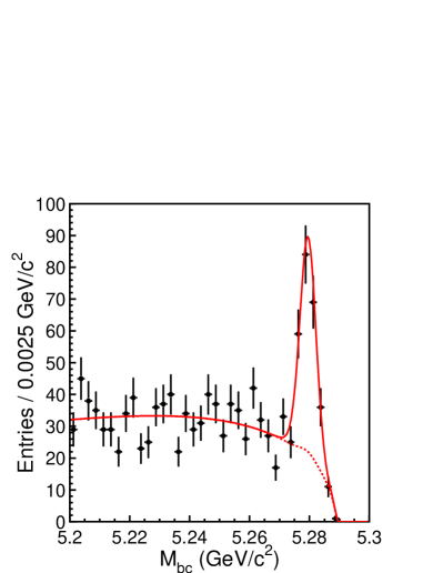
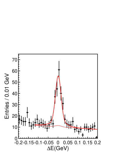
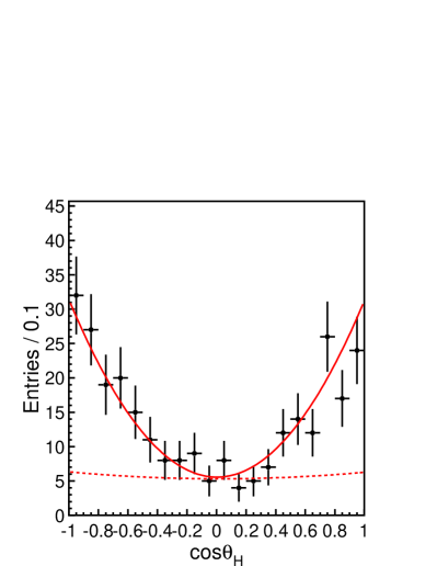
Figure 1: Distributions of (a) ${M_{\rm bc}}$ in the ${\Delta E}$ signal region, (b) ${\Delta E}$ in the ${M_{\rm bc}}$ signal region and (c) $\cos\theta_{H}$ in the ${\Delta E}$-${M_{\rm bc}}$ signal region for ${B^{0}}\to\phi{K_{S}^{0}}$ candidates. Solid curves show the fits to signal plus background distributions, and dashed curves show the background contributions.

The signal yield for the ${B^{0}}\to\phi{K_{S}^{0}}$ decay is determined from an unbinned three-dimensional maximum-likelihood fit to the ${\Delta E}$-${M_{\rm bc}}$-$\cos\theta_{H}$ distribution footnote:costhetaH . The fit region is defined as $-0.12~{}{\rm GeV}<{\Delta E}<0.25~{}{\rm GeV}$ for the ${K_{S}^{0}}\to{\pi^{+}}{\pi^{-}}$ channel, $-0.25~{}{\rm GeV}<{\Delta E}<0.25~{}{\rm GeV}$ for the ${K_{S}^{0}}\to{\pi^{0}}{\pi^{0}}$ channel and ${M_{\rm bc}}>5.2~{}{\rm GeV/}c^{2}$ for both cases. The signal distribution for $\phi{K_{S}^{0}}~{}({K_{S}^{0}}\to{\pi^{+}}{\pi^{-}})$ is modeled with a Gaussian function (a sum of two Gaussian functions) for ${M_{\rm bc}}$ (${\Delta E}$). The $\phi{K_{S}^{0}}~{}({K_{S}^{0}}\to{\pi^{0}}{\pi^{0}})$ signal distribution is modeled with a smoothed histogram obtained from MC events. For the continuum background, we use the ARGUS parameterization bib:ARGUS for ${M_{\rm bc}}$ and a linear function for ${\Delta E}$. Finally, the $\cos\theta_{H}$ distribution for the ${B^{0}}\to\phi{K_{S}^{0}}$ signal (continuum) is modeled with a second-order polynomial and is determined from MC (events in the ${\Delta E}$-${M_{\rm bc}}$ sideband). The $\cos\theta_{H}$ distribution for the non-resonant ${B^{0}}\to{K^{+}}{K^{-}}{K_{S}^{0}}$ background is also determined from MC and is included in the fit, with a ratio between the non-resonant component and the $\phi{K_{S}^{0}}$ signal fixed at the measured value. The fits yield a total of $180\pm 16$(stat) ${B^{0}}\to\phi{K_{S}^{0}}$ events in the signal region.

Figures 2(a) and (b) show distributions of ${M_{\rm bc}}$ in the ${\Delta E}$ signal region and ${\Delta E}$ in the ${M_{\rm bc}}$ signal region for the reconstructed ${B^{0}}\to{K^{+}}{K^{-}}{K_{S}^{0}}$ candidates after flavor tagging and vertex reconstruction.

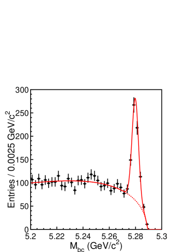
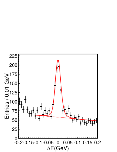
Figure 2: Distributions of (a) ${M_{\rm bc}}$ within the ${\Delta E}$ signal region, (b) ${\Delta E}$ within the ${M_{\rm bc}}$ signal region for ${B^{0}}\to{K^{+}}{K^{-}}{K_{S}^{0}}$ candidates. Solid curves show the fits to signal plus background distributions, and dashed curves show the background contributions.

The signal yield for the ${B^{0}}\to{K^{+}}{K^{-}}{K_{S}^{0}}$ decay is determined from an unbinned two-dimensional maximum-likelihood fit to the ${\Delta E}$-${M_{\rm bc}}$ distribution in the fit region defined as $-0.12~{}{\rm GeV}<{\Delta E}<0.25~{}{\rm GeV}$ and ${M_{\rm bc}}>5.2~{}{\rm GeV/}c^{2}$. The signal and background distributions are modeled in the same way as the ${B^{0}}\to\phi{K_{S}^{0}}~{}({K_{S}^{0}}\to{\pi^{+}}{\pi^{-}})$ case. The fit yields $536\pm 29$(stat) ${B^{0}}\to{K^{+}}{K^{-}}{K_{S}^{0}}$ events in the signal region.

II.3 ${B^{0}}\to\phi{K_{L}^{0}}$

Candidate $\phi\to{K^{+}}{K^{-}}$ decays are selected with the criteria described above. We select ${K_{L}^{0}}$ candidates based on KLM and ECL information. There are three classes of ${K_{L}^{0}}$ candidates, which we refer to as KLM, ECL and KLM+ECL candidates. The KLM candidates are selected from hit clusters in the KLM that are not associated with either an ECL cluster nor with a charged track. The requirements for the KLM candidates are the same as those used in the ${B^{0}}\to{J/\psi}{K_{L}^{0}}$ selection for our previous ${\sin 2\phi_{1}}$ measurement bib:CP1_Belle . ECL candidates are selected from ECL clusters if there is no KLM candidate. We use a ${K_{L}^{0}}$ likelihood ratio bib:CP1_Belle , which is calculated from the following information: the distance between the ECL cluster and the closest extrapolated charged track position; the ECL cluster energy; $E_{9}/E_{25}$, the ratio of energies summed in $3\times 3$ and $5\times 5$ arrays of CsI(Tl) crystals surrounding the crystal at the center of the shower; the ECL shower width and the invariant mass of the shower. The likelihood ratio is required to be greater than 0.69. A KLM+ECL candidate is an ECL cluster with cluster energy greater than 0.16 GeV that has an associated KLM cluster. Here we impose less stringent requirements than those for KLM candidates to select the cluster in the KLM detector. The ${K_{L}^{0}}$ likelihood ratio for the ECL cluster is required to be greater than 0.56. For all KLM, KLM+ECL and ECL candidates, we also require that the cosine of the angle between the ${K_{L}^{0}}$ direction and the direction of the missing momentum of the event in the laboratory frame be greater than 0.6.

Since the energy of the ${K_{L}^{0}}$ is not measured, ${M_{\rm bc}}$ and ${\Delta E}$ cannot be calculated in the same way as for the other final states. Using the four-momentum of a reconstructed $\phi$ candidate and the ${K_{L}^{0}}$ flight direction, we calculate the momentum of the ${K_{L}^{0}}$ candidate requiring ${\Delta E}=0$. We then calculate $p_{B}^{\rm cms}$, the momentum of the $B$ candidate in the cms, and define the $B$ meson signal region as $0.2~{}{\rm GeV/}c<p_{B}^{\rm cms}<0.5~{}{\rm GeV/}c$. We impose the requirement ${\cal R}_{\rm s/b}>0.80$, which rejects 95.7% of the continuum background and 67.0% of backgrounds from $B$ decays, while retaining 65.2% of signal events. Here ${\cal R}_{\rm s/b}$ is based on the discriminating variables used for the ${B^{0}}\to\phi{K_{S}^{0}}$ decay and the number of tracks originating from the IP with a momentum above 0.1 GeV/$c$. We exclusively reconstruct and reject ${B^{0}}\to{K^{+}}{K^{-}}{K_{S}^{0}}$ (including $\phi\to{K^{+}}{K^{-}}$ and ${f_{0}}\to{K^{+}}{K^{-}})$, $\phi{K^{*0}}$ $({K^{*0}}\to{K^{+}}{\pi^{-}}$ or ${K_{S}^{0}}{\pi^{0}})$, $\phi{\pi^{0}}$, $\phi\eta$, ${B^{+}}\to\phi{K^{+}}$, and $\phi{K^{*+}}$ $({K^{*+}}\to{K_{S}^{0}}{\pi^{+}}$ or ${K^{+}}{\pi^{0}})$ decays. If there is more than one candidate ${B^{0}}\to\phi{K_{L}^{0}}$ decay in the signal region, priority is given to KLM candidates. If there still exist multiple candidates, we take the one with the ${K_{L}^{0}}$ candidate closest to the expected ${K_{L}^{0}}$ direction.

We study the background components using a large MC sample as well as data taken with cms energy 60 MeV below the nominal $\Upsilon(4S)$ mass (off-resonance data). The dominant background is from continuum. A MC study shows that background events from $B$ decays are dominated by inclusive $B\to\phi{K_{L}^{0}}X$ decays that include $B\to\phi K^{*}$ decays.

The signal yield is determined from an extended three-dimensional binned maximum-likelihood fit to the ${\cal R}_{\rm s/b}$-$p_{B}^{\rm cms}$-$r$ distribution in the fit region $0.8<{\cal R}_{\rm s/b}\leq 1.0$, $0~{}{\rm GeV/}c<p_{B}^{\rm cms}\leq 0.6~{}{\rm GeV/}c$ and $r>0.25$, where the total likelihood is a product of the likelihood for each of three variables. The ${B^{0}}\to\phi{K_{L}^{0}}$ signal shape is obtained from MC events. Background from $B{\overline{B}}$ pairs is also modeled with MC. We fix the ratio between the signal and the $B{\overline{B}}$ background based on known branching fractions and MC-determined reconstruction efficiencies with the ${K_{L}^{0}}$ detection efficiency corrected from ${B^{0}}\to{J/\psi}{K_{L}^{0}}$ data. The uncertainty in the ratio is treated as a source of systematic error. The continuum background distribution is represented by a histogram obtained from MC events; we confirm that the function well describes both the off-resonance data and the events in a $p_{B}^{\rm cms}$ sideband region defined as $1.0~{}{\rm GeV/}c<p_{B}^{\rm cms}\leq 1.6~{}{\rm GeV/}c$. The fit yields $78\pm 13$ ${B^{0}}\to\phi{K_{L}^{0}}$ events, where the error is statistical only. The result is in agreement with the expected ${B^{0}}\to\phi{K_{L}^{0}}$ signal yield (59 events) obtained from MC after applying the efficiency correction from the ${B^{0}}\to{J/\psi}{K_{L}^{0}}$ data. Figure 3(a) shows the ${\cal R}_{\rm s/b}$ distribution in the $p_{B}^{\rm cms}$-$r$ signal region. Figure 3(b) shows signal yields obtained for six $p_{B}^{\rm cms}$ intervals separately. The yields agree with the distribution obtained by the three-dimensional fit.

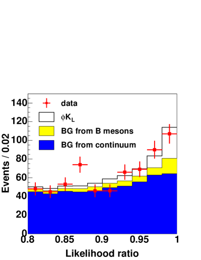
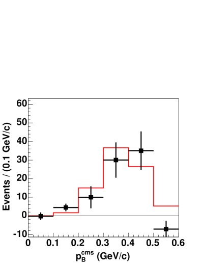
Figure 3: (a) Distribution of ${\cal R}_{\rm s/b}$ in the $p_{B}^{\rm cms}$ signal region. The solid histogram shows the fit to the signal plus background distribution, and the shaded histograms show the background contributions. (b) Background-subtracted $p_{B}^{\rm cms}$ distribution for ${B^{0}}\to\phi{K_{L}^{0}}$ candidates. The solid histogram shows the result of the three-dimensional fit to the ${\cal R}_{\rm s/b}$-$p_{B}^{\rm cms}$-$r$ distribution.

II.4 ${B^{0}}\to\eta^{\prime}{K_{S}^{0}}$

Candidate ${K_{S}^{0}}\to{\pi^{+}}{\pi^{-}}$ and ${\pi^{0}}{\pi^{0}}$ decays are selected with the same criteria as those used for the ${B^{0}}\to\phi{K_{S}^{0}}$ decay. Charged pions from the $\eta$, ${\rho^{0}}$ or $\eta^{\prime}$ decay are selected from tracks originating from the IP. We reject kaon candidates by requiring ${\cal R}_{K/\pi}<0.9$. Candidate photons from ${\pi^{0}}\to\gamma\gamma$ decays are required to have $E_{\gamma}>0.05$ GeV. The reconstructed ${\pi^{0}}$ candidate is required to satisfy $0.118~{}{\rm GeV}/c^{2}<M_{\gamma\gamma}<0.15~{}{\rm GeV}/c^{2}$ and $p_{\pi^{0}}^{\rm cms}>0.1~{}{\rm GeV}/c$, where $M_{\gamma\gamma}$ and $p_{\pi^{0}}^{\rm cms}$ are the invariant mass and the momentum in the cms, respectively. Candidate photons from $\eta\to\gamma\gamma~{}(\eta^{\prime}\to{\rho^{0}}\gamma)$ decays are required to have $E_{\gamma}>0.05~{}(0.1)$ GeV. The invariant mass of the photon pair is required to be between 0.5 and 0.57 GeV/$c^{2}$ for the $\eta\to\gamma\gamma$ decay. The ${\pi^{+}}{\pi^{-}}{\pi^{0}}$ invariant mass is required to be between 0.535 and 0.558 GeV/$c^{2}$ for the $\eta\to{\pi^{+}}{\pi^{-}}{\pi^{0}}$ decay, which is used only for the reconstruction of the ${B^{0}}\to{\eta^{\prime}}{K_{S}^{0}}~{}({K_{S}^{0}}\to{\pi^{+}}{\pi^{-}})$ decay. A kinematic fit with an $\eta$ mass constraint is performed using the fitted vertex of the $\pi^{+}\pi^{-}$ tracks from the $\eta^{\prime}$ as the decay point. For $\eta^{\prime}\to{\rho^{0}}\gamma$ decays, candidate ${\rho^{0}}$ mesons are reconstructed from pairs of vertex-constrained $\pi^{+}\pi^{-}$ tracks with invariant mass between 0.55 and 0.92 GeV/$c^{2}$. The $\eta^{\prime}\to\eta{\pi^{+}}{\pi^{-}}$ candidates are required to have a reconstructed mass between 0.94 and 0.97 GeV/$c^{2}$ (0.95 and 0.966 GeV/$c^{2}$) for the $\eta\to\gamma\gamma$ ($\eta\to{\pi^{+}}{\pi^{-}}{\pi^{0}}$) decay. Candidate $\eta^{\prime}\to{\rho^{0}}\gamma$ decays are required to have a reconstructed mass from 0.935 to 0.975 GeV/$c^{2}$.

The $B$ meson signal region is defined as $|{\Delta E}|<0.06$ GeV for ${B^{0}}\to\eta^{\prime}{K_{S}^{0}}~{}(\eta^{\prime}\to{\rho^{0}}\gamma,~{}{K_{S}^{0}}\to{\pi^{+}}{\pi^{-}})$, $-0.1$ GeV $<{\Delta E}<0.08$ GeV for ${B^{0}}\to\eta^{\prime}{K_{S}^{0}}~{}(\eta^{\prime}\to\eta{\pi^{+}}{\pi^{-}},~{}\eta\to\gamma\gamma,~{}{K_{S}^{0}}\to{\pi^{+}}{\pi^{-}})$, $-0.08$ GeV $<{\Delta E}<0.06$ GeV for ${B^{0}}\to\eta^{\prime}{K_{S}^{0}}~{}(\eta^{\prime}\to\eta{\pi^{+}}{\pi^{-}},~{}\eta\to{\pi^{+}}{\pi^{-}}{\pi^{0}},~{}{K_{S}^{0}}\to{\pi^{+}}{\pi^{-}})$, $-0.15$ GeV $<{\Delta E}<0.1$ GeV for ${B^{0}}\to\eta^{\prime}{K_{S}^{0}}~{}({K_{S}^{0}}\to{\pi^{0}}{\pi^{0}})$, and $5.27~{}{\rm GeV}/c^{2}<{M_{\rm bc}}<5.29~{}{\rm GeV}/c^{2}$ for all decays. The continuum suppression is based on the likelihood ratio ${\cal R}_{\rm s/b}$ obtained from the same discriminating variables used for the ${B^{0}}\to\phi{K_{S}^{0}}$ decay, except for the decay mode $\eta^{\prime}\to\rho\gamma~{}(\rho\to{\pi^{+}}{\pi^{-}})$ where $\cos\theta_{H}$ is included. Here $\theta_{H}$ is defined as the angle between the $\eta^{\prime}$ meson momentum and the daughter ${\pi^{+}}$ momentum in the $\rho$ meson rest frame. The minimum ${\cal R}_{\rm s/b}$ requirement depends both on the decay mode and on the flavor-tagging quality, and ranges from 0 (i.e., no requirement) to $0.4$ for the decay ${B^{0}}\to{\eta^{\prime}}{K_{S}^{0}}~{}({K_{S}^{0}}\to{\pi^{+}}{\pi^{-}})$ and from 0.2 to 0.9 for the decay ${B^{0}}\to{\eta^{\prime}}{K_{S}^{0}}~{}({K_{S}^{0}}\to{\pi^{0}}{\pi^{0}})$. For the $\eta^{\prime}\to{\rho^{0}}\gamma$ mode, we also require $|\cos\theta_{T}|<0.9$ prior to the ${\cal R}_{\rm s/b}$ requirement. With these requirements, the continuum background in the ${B^{0}}\to{\eta^{\prime}}{K_{S}^{0}}~{}({K_{S}^{0}}\to{\pi^{+}}{\pi^{-}})$ mode is reduced by 87% for $\eta^{\prime}\to{\rho^{0}}\gamma$, 58% for $\eta^{\prime}\to\eta{\pi^{+}}{\pi^{-}}~{}(\eta\to\gamma\gamma)$ and 31% for $\eta^{\prime}\to\eta{\pi^{+}}{\pi^{-}}~{}(\eta\to{\pi^{+}}{\pi^{-}}{\pi^{0}})$, while retaining 78% of the signal for $\eta^{\prime}\to{\rho^{0}}\gamma$, 94% for $\eta^{\prime}\to\eta{\pi^{+}}{\pi^{-}}~{}(\eta\to\gamma\gamma)$ and 97% for $\eta^{\prime}\to\eta{\pi^{+}}{\pi^{-}}~{}(\eta\to{\pi^{+}}{\pi^{-}}{\pi^{0}})$. The continuum background for the ${B^{0}}\to{\eta^{\prime}}{K_{S}^{0}}~{}({K_{S}^{0}}\to{\pi^{0}}{\pi^{0}})$ candidates is reduced by 90% (97%) while retaining 81% (54%) of signal events for ${\eta^{\prime}}\to\eta{\pi^{+}}{\pi^{-}}~{}(\rho\gamma)$.

We use events outside the signal region as well as a large MC sample to study the background components in ${B^{0}}\to{\eta^{\prime}}{K_{S}^{0}}$. The dominant background is from continuum. In addition, according to MC simulation, there is a small ($\sim 3\%$) combinatorial background from $B\overline{B}$ events in ${B^{0}}\to\eta^{\prime}{K_{S}^{0}}~{}(\eta^{\prime}\to{\rho^{0}}\gamma)$. The contributions from $B\overline{B}$ events are smaller for other modes. The influence of these backgrounds is treated as a source of systematic uncertainty.

Figure 4(a) shows the ${M_{\rm bc}}$ distribution for the reconstructed ${B^{0}}\to\eta^{\prime}{K_{S}^{0}}$ candidates within the ${\Delta E}$ signal region after flavor tagging and vertex reconstruction, where all subdecay modes are combined. The ${\Delta E}$ distribution for the ${B^{0}}\to\eta^{\prime}{K_{S}^{0}}$ candidates within the ${M_{\rm bc}}$ signal region is shown in Fig. 4(b).

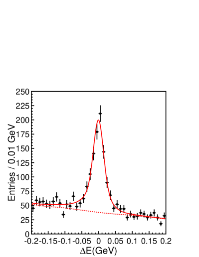
Figure 4: Distributions of (a) ${M_{\rm bc}}$ within the ${\Delta E}$ signal region, (b) ${\Delta E}$ within the ${M_{\rm bc}}$ signal region for ${B^{0}}\to{\eta^{\prime}}{K_{S}^{0}}$ candidates. Solid curves show the fits to signal plus background distributions, and dashed curves show the background contributions.

The signal yields are determined from unbinned two-dimensional maximum-likelihood fits to the ${\Delta E}$-${M_{\rm bc}}$ distributions. The fit region is defined as $-0.25~{}{\rm GeV}<{\Delta E}<0.25~{}{\rm GeV}$ and ${M_{\rm bc}}>5.2~{}{\rm GeV/}c^{2}$. We perform the fit for each final state separately. The $\eta^{\prime}{K_{S}^{0}}~{}({K_{S}^{0}}\to{\pi^{+}}{\pi^{-}})$ signal distribution is modeled with a sum of two (three) Gaussian functions for ${M_{\rm bc}}$ (${\Delta E}$). The $\eta^{\prime}{K_{S}^{0}}~{}({K_{S}^{0}}\to{\pi^{0}}{\pi^{0}})$ signal distribution is modeled with a smoothed histogram. For the continuum background, we use the ARGUS parameterization for ${M_{\rm bc}}$ and a linear function for ${\Delta E}$. For the $\eta^{\prime}\to\rho\gamma$ mode, we include in the fits the $B{\overline{B}}$ background shape obtained from MC. The fits yield a total of $830\pm 35$ ${B^{0}}\to\eta^{\prime}{K_{S}^{0}}$ events in the signal region, where the error is statistical only.

II.5 ${B^{0}}\to\eta^{\prime}{K_{L}^{0}}$

Candidate ${\eta^{\prime}}\to\eta{\pi^{+}}{\pi^{-}}$ $(\eta\to\gamma\gamma)$ decays are selected with the same criteria as those used for the ${B^{0}}\to{\eta^{\prime}}{K_{S}^{0}}$ analysis. The ${K_{L}^{0}}$ selection is adopted from the $\phi{K_{L}^{0}}$ analysis, with a likelihood ratio optimized for the ${B^{0}}\to{\eta^{\prime}}{K_{L}^{0}}$ decay that is required to be greater than 0.50 (0.40) for KLM+ECL (ECL) candidates. The best candidate is formed from the ${\eta^{\prime}}$ candidate with the smallest $\chi^{2}$ value in its mass-constrained fit and the ${K_{L}^{0}}$ candidate whose measured direction is closest to the expected direction. The following exclusive modes are reconstructed and are rejected: $B\to{\eta^{\prime}}{\pi^{0}}$, ${\eta^{\prime}}\pi^{\pm}$, ${\eta^{\prime}}\eta$, ${\eta^{\prime}}{K_{S}^{0}}$, ${\eta^{\prime}}K^{\pm}$, ${\eta^{\prime}}K^{*0}$ $(\to{K_{S}^{0}}{\pi^{0}}$ or $K^{\pm}\pi^{\mp})$, ${\eta^{\prime}}K^{*\pm}$, ${\eta^{\prime}}\rho^{0}$ and ${\eta^{\prime}}\rho^{\pm}$. The $B$ meson signal region is defined as ${\cal R}_{\rm s/b}>0.8$, $0.2~{}{\rm GeV/}c<p_{B}^{\rm cms}<0.5~{}{\rm GeV/}c$ and $r>0.25$ (0.5 for ECL candidates).

The signal yield is determined from an extended three-dimensional maximum-likelihood fit to the ${\cal R}_{\rm s/b}$-$p_{B}^{\rm cms}$-$r$ distribution. The procedure to determine the signal and background distributions is the same as that for the ${B^{0}}\to\phi{K_{L}^{0}}$ decay. The fit yields $187\pm 18$ ${B^{0}}\to{\eta^{\prime}}{K_{L}^{0}}$ events, where the error is statistical only. The result is in good agreement with the expected ${B^{0}}\to{\eta^{\prime}}{K_{L}^{0}}$ signal yield (180 events) obtained from MC after applying the efficiency correction from the ${B^{0}}\to{J/\psi}{K_{L}^{0}}$ data. Figure 5(a) shows the ${\cal R}_{\rm s/b}$ distribution in the $p_{B}^{\rm cms}$-$r$ signal region. Figure 5(b) shows signal yields obtained for twelve $p_{B}^{\rm cms}$ intervals separately. The yields agree with the distribution obtained by the three-dimensional fit.

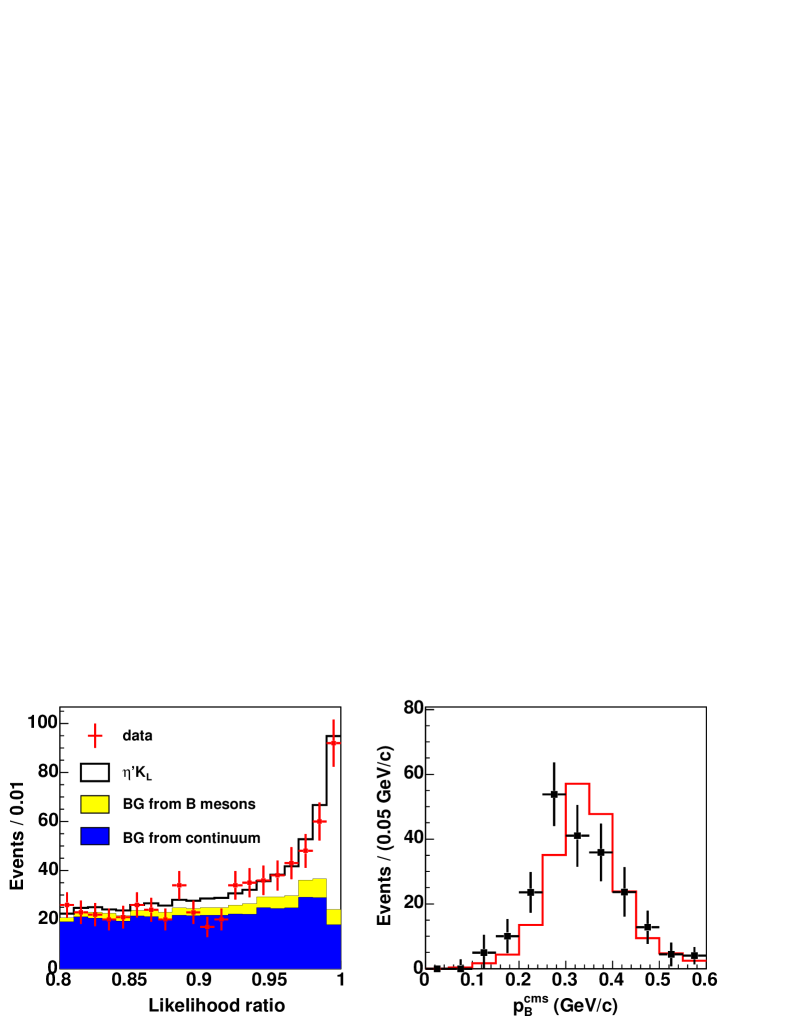
Figure 5: Distributions of (a) ${\cal R}_{\rm s/b}$ in the $p_{B}^{\rm cms}$ signal region and (b) background-subtracted $p_{B}^{\rm cms}$ for ${B^{0}}\to{\eta^{\prime}}{K_{L}^{0}}$ candidates. Solid histograms show the fits to signal plus background distributions, and the shaded histogram shows the background contributions.

II.6 ${B^{0}}\to{K_{S}^{0}}{K_{S}^{0}}{K_{S}^{0}}$

We reconstruct the ${B^{0}}\to{K_{S}^{0}}{K_{S}^{0}}{K_{S}^{0}}$ decay in the ${K_{S}^{+-}}{K_{S}^{+-}}{K_{S}^{+-}}$ or ${K_{S}^{+-}}{K_{S}^{+-}}{K_{S}^{00}}$ final state, where the ${\pi^{+}}{\pi^{-}}$ (${\pi^{0}}{\pi^{0}}$) state from a ${K_{S}^{0}}$ decay is denoted as ${K_{S}^{+-}}$ (${K_{S}^{00}}$). Pairs of oppositely charged tracks with ${\pi^{+}}{\pi^{-}}$ invariant mass within 0.012 GeV/$c^{2}$ ($\simeq 3\sigma$) of the nominal ${K_{S}^{0}}$ mass are used to reconstruct ${K_{S}^{+-}}$ candidates. The ${\pi^{+}}{\pi^{-}}$ vertex is required to be displaced from the interaction point (IP) by a minimum transverse distance of 0.22 cm for ${K_{S}^{0}}$ candidates with momentum greater than 1.5 GeV/$c$ and 0.08 cm for those with momentum less than 1.5 GeV/$c$. The angle in the transverse plane between the ${K_{S}^{0}}$ momentum vector and the direction defined by the ${K_{S}^{0}}$ vertex and the IP should be less than 0.03 rad (0.1 rad) for the high (low) momentum candidates. The mismatch in the $z$ direction at the ${K_{S}^{0}}$ vertex point for the two charged pion tracks should be less than 2.4 cm (1.8 cm) for the high (low) momentum candidates. After two good ${K_{S}^{+-}}$ candidates have been found that satisfy the criteria given above, looser requirements are applied for the third ${K_{S}^{+-}}$ candidate. The requirement on the transverse direction matching is relaxed to 0.2 rad (0.4 rad for low momentum candidates), and the mismatch of the two charged pions in the $z$ direction is required to be less than 5 cm (1 cm if both pions have hits in the SVD). We also require that the ${K_{S}^{0}}$ flight length in the plane perpendicular to the beam axis be less than 0.5 mm and the ${K_{S}^{0}}$ momentum be greater than 0.5 GeV/$c$.

To select ${K_{S}^{00}}$ candidates, we reconstruct ${\pi^{0}}$ candidates from pairs of photons with $E_{\gamma}>0.05$ GeV. The reconstructed ${\pi^{0}}$ candidate is required to have an invariant mass between 0.08 and 0.15 GeV/$c^{2}$ and momentum above 0.1 GeV/$c$. ${K_{S}^{00}}$ candidates are required to have an invariant mass between 0.47 and 0.52 GeV/$c^{2}$, and a fit is performed with constraints on the ${K_{S}^{0}}$ vertex and ${\pi^{0}}$ masses to improve the ${\pi^{0}}{\pi^{0}}$ invariant mass resolution. The ${K_{S}^{00}}$ candidate is combined with two good ${K_{S}^{+-}}$ candidates to reconstruct a ${B^{0}}$ meson.

The ${B^{0}}$ meson signal region is defined as $|{\Delta E}|<0.10$ GeV for ${B^{0}}\to{K_{S}^{+-}}{K_{S}^{+-}}{K_{S}^{+-}}$, $-0.15~{}{\rm GeV}<{\Delta E}<0.10$ GeV for ${B^{0}}\to{K_{S}^{+-}}{K_{S}^{+-}}{K_{S}^{00}}$, and $5.27~{}{\rm GeV}/c^{2}<{M_{\rm bc}}<5.29~{}{\rm GeV}/c^{2}$ for both decays. To suppress the $e^{+}e^{-}\rightarrow q\overline{q}$ continuum background ($q=u,~{}d,~{}s,~{}c$), we form the likelihood ratio ${\cal R}_{\rm s/b}$ by combining likelihoods for two quantities; a Fisher discriminant of modified Fox-Wolfram moments, and the cosine of the cms ${B^{0}}$ flight direction.The requirement for ${\cal R}_{\rm s/b}$ depends both on the decay mode and on the flavor-tagging quality; after applying all other cuts, this requirement rejects 94% of the $q\bar{q}$ background while retaining 75% of the signal.

If both ${B^{0}}\to{K_{S}^{+-}}{K_{S}^{+-}}{K_{S}^{+-}}$ and ${K_{S}^{+-}}{K_{S}^{+-}}{K_{S}^{00}}$ candidates are found in the same event, we choose the ${B^{0}}\to{K_{S}^{+-}}{K_{S}^{+-}}{K_{S}^{+-}}$ candidate. If more than one ${B^{0}}\to{K_{S}^{+-}}{K_{S}^{+-}}{K_{S}^{+-}}$ candidate is found, we check for each of them the quality of the third ${K_{S}^{+-}}$ candidate, which is selected with looser requirements as described above. We choose the ${B^{0}}\to{K_{S}^{+-}}{K_{S}^{+-}}{K_{S}^{+-}}$ candidate in which the third ${K_{S}^{+-}}$ candidate satisfies the tight ${K_{S}^{+-}}$ selection requirements. If no ${B^{0}}$ candidate is found with the tight requirements or more than one ${B^{0}}$ candidate still remain, we select the one with the smallest value for $\sum(\Delta M_{{K_{S}^{+-}}})^{2}$, where $\Delta M_{{K_{S}^{+-}}}$ is the difference between the reconstructed and nominal mass of ${K_{S}^{+-}}$. For multiple ${B^{0}}\to{K_{S}^{+-}}{K_{S}^{+-}}{K_{S}^{00}}$ candidates, we select the ${K_{S}^{+-}}{K_{S}^{+-}}$ pair that has the smallest $\sum(\Delta M_{{K_{S}^{+-}}})^{2}$ value and the ${K_{S}^{00}}$ candidate with the minimum $\chi^{2}$ of the constrained fit.

We reject ${K_{S}^{0}}{K_{S}^{0}}{K_{S}^{0}}$ candidates if they are consistent with ${B^{0}}\to\chi_{c0}{K_{S}^{0}}\to({K_{S}^{0}}{K_{S}^{0}}){K_{S}^{0}}$ or ${B^{0}}\to D^{0}{K_{S}^{0}}\to({K_{S}^{0}}{K_{S}^{0}}){K_{S}^{0}}$ decays, i.e. if one of the ${K_{S}^{0}}$ pairs has an invariant mass within $\pm 2\sigma$ of the $\chi_{c0}$ mass or $D^{0}$ mass, where $\sigma$ is the ${K_{S}^{0}}{K_{S}^{0}}$ mass resolution.

We use events outside the signal region as well as a large MC sample to study the background components. The dominant background is from continuum. The contamination of ${B^{0}}\to\chi_{c0}{K_{S}^{0}}$ events in the ${B^{0}}\to{K_{S}^{0}}{K_{S}^{0}}{K_{S}^{0}}$ sample is small. The contributions from other $B\overline{B}$ events are negligibly small. The influence of these backgrounds is treated as a source of systematic uncertainty in the $CP$ asymmetry measurement. Backgrounds from the decay ${B^{0}}\to D^{0}{K_{S}^{0}}$ are found to be negligible.

Figure 6 shows the ${M_{\rm bc}}$ and ${\Delta E}$ distributions for the reconstructed ${B^{0}}\to{K_{S}^{0}}{K_{S}^{0}}{K_{S}^{0}}$ candidates after flavor tagging and vertex reconstruction. The signal yield is determined from an unbinned two-dimensional maximum-likelihood fit to the ${\Delta E}$-${M_{\rm bc}}$ distribution. The ${K_{S}^{+-}}{K_{S}^{+-}}{K_{S}^{+-}}$ signal distribution is modeled with a Gaussian function (a sum of two Gaussian functions) for ${M_{\rm bc}}$ (${\Delta E}$). For ${B^{0}}\to{K_{S}^{+-}}{K_{S}^{+-}}{K_{S}^{00}}$ decay, the signal is modeled with a two-dimensional smoothed histogram obtained from MC events. For the continuum background, we use the ARGUS parameterization for ${M_{\rm bc}}$ and a linear function for ${\Delta E}$. The fits after flavor tagging and vertex reconstruction yield $88\pm 10$ ${B^{0}}\to{K_{S}^{+-}}{K_{S}^{+-}}{K_{S}^{+-}}$ events and $16\pm 6$ ${B^{0}}\to{K_{S}^{+-}}{K_{S}^{+-}}{K_{S}^{00}}$ events for a total of $105\pm 12$ ${B^{0}}\to{K_{S}^{0}}{K_{S}^{0}}{K_{S}^{0}}$ events in the signal region, where the errors are statistical only. The obtained purity is $0.70$ for the ${K_{S}^{+-}}{K_{S}^{+-}}{K_{S}^{+-}}$ and $0.43$ for the ${K_{S}^{+-}}{K_{S}^{+-}}{K_{S}^{00}}$ channels. Here the purity is defined as ${N_{\rm sig}}/{N_{\rm ev}}$, where ${N_{\rm sig}}$ is the number of signal events in the signal region obtained by the fit, and ${N_{\rm ev}}$ is the total number of events in the signal region.

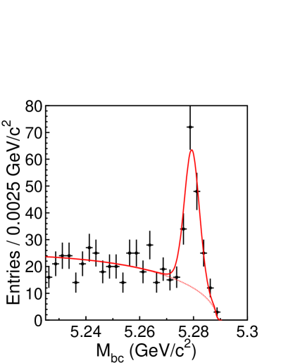
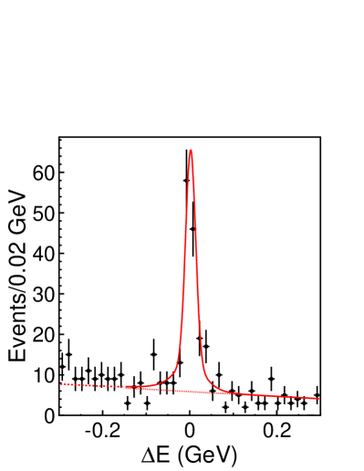
Figure 6: Distributions of (a) ${M_{\rm bc}}$ within the ${\Delta E}$ signal region, (b) ${\Delta E}$ within the ${M_{\rm bc}}$ signal region for ${B^{0}}\to{K_{S}^{0}}{K_{S}^{0}}{K_{S}^{0}}$ candidates. Solid curves show the fits to signal plus background distributions, and dashed curves show the background contributions.

II.7 ${B^{0}}\to{K_{S}^{0}}{\pi^{0}}$

Candidate ${K_{S}^{0}}\to{\pi^{+}}{\pi^{-}}$ decays are selected with the same criteria as those used for the ${B^{0}}\to\phi{K_{S}^{0}}$ decay, except that we use pairs of oppositely charged pions that have an invariant mass within 0.018 GeV/$c^{2}$ of the nominal ${K_{S}^{0}}$ mass. The ${\pi^{0}}$ selection criteria are the same as those used for the ${B^{0}}\to\eta^{\prime}{K_{S}^{0}}$ decay.

The $B$ meson signal region is defined as $-0.15$ GeV $<{\Delta E}<0.1$ GeV and $5.27~{}{\rm GeV}/c^{2}<{M_{\rm bc}}<5.29~{}{\rm GeV}/c^{2}$. The ${\Delta E}$ distribution for ${K_{S}^{0}}{\pi^{0}}$ has a tail toward lower ${\Delta E}$. The ${\Delta E}$ resolution is 0.047 GeV for the main component. The width of the tail is about 0.1 GeV. The dominant background is from continuum. In addition, according to MC simulation, there is a small ($\sim 2\%$) contamination from other charmless rare $B$ decays. We use extended modified Fox-Wolfram moments, which were applied for the selection of the ${B^{0}}\to{\pi^{0}}{\pi^{0}}$ decay Chen:2005dr , to form a Fisher discriminant ${\cal F}$. We then combine likelihoods for ${\cal F}$ and $\cos\theta_{B}$ to obtain the event likelihood ratio ${\cal R}_{\rm s/b}$ for continuum suppression.

As described below, we include events that do not have $B$ decay vertex information in our fit to obtain a better sensitivity for the $CP$-violation parameter ${\cal A}_{f}$. For events with and without vertex information, the high-${\cal R}_{\rm s/b}$ region is defined as ${\cal R}_{\rm s/b}>0.8$ and the low-${\cal R}_{\rm s/b}$ region as $0.45<{\cal R}_{\rm s/b}\leq 0.8$ for both DS-I and DS-II. After applying the high-${\cal R}_{\rm s/b}$ requirement, 95% of the continuum background is rejected and 62% of signal events remain. In the low-${\cal R}_{\rm s/b}$ region, 84% of the continuum background is rejected and 24% of the signal remains.

Figure 7(a) shows the ${M_{\rm bc}}$ distribution for the ${B^{0}}\to{K_{S}^{0}}{\pi^{0}}$ candidates within the ${\Delta E}$ signal region after flavor tagging and before vertex reconstruction. Also shown in Fig. 7(b) is the ${\Delta E}$ distribution within the ${M_{\rm bc}}$ signal region.

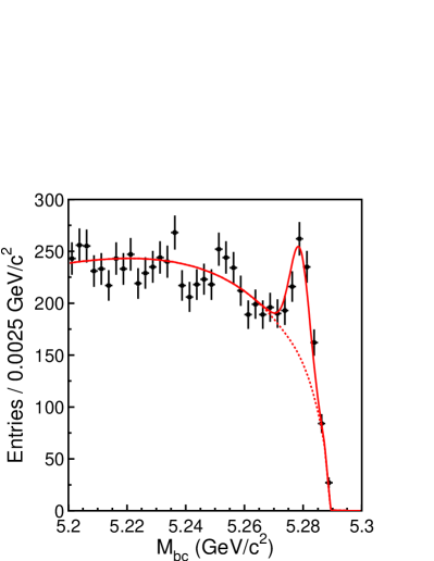
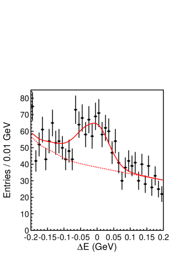
Figure 7: Distributions of (a) ${M_{\rm bc}}$ within the ${\Delta E}$ signal region, (b) ${\Delta E}$ within the ${M_{\rm bc}}$ signal region for ${B^{0}}\to{K_{S}^{0}}{\pi^{0}}$ candidates. Solid curves show the fits to signal plus background distributions, and dashed curves show the background contributions.

The signal yield is determined from an unbinned two-dimensional maximum-likelihood fit to the ${\Delta E}$-${M_{\rm bc}}$ distribution in the fit region defined as $5.2~{}{\rm GeV/}c^{2}<{M_{\rm bc}}<5.29~{}{\rm GeV/}c^{2}$ and $-0.3~{}{\rm GeV}<{\Delta E}<0.3~{}{\rm GeV}$. The ${B^{0}}\to{K_{S}^{0}}{\pi^{0}}$ signal distribution is modeled with a smoothed histogram obtained from MC and calibrated with data using ${B^{-}}\to D^{0}{\pi^{-}}$ $(D^{0}\to{K^{-}}{\pi^{+}}{\pi^{0}})$. For the continuum background, we use the ARGUS parameterization for ${M_{\rm bc}}$ and a linear function for ${\Delta E}$. The $B$ decay background distribution is represented by a smoothed histogram obtained from MC simulation. The fits yield $248\pm 20$ and $96\pm 23$ ${B^{0}}\to{K_{S}^{0}}{\pi^{0}}$ events in the high-${\cal R}_{\rm s/b}$ and low-${\cal R}_{\rm s/b}$ signal regions, respectively, where the errors are statistical only. The same procedure after the vertex reconstruction yields a total of $106\pm 14$ ${K_{S}^{0}}{\pi^{0}}$ events.

II.8 ${B^{0}}\to{f_{0}}{K_{S}^{0}}$

Candidate ${K_{S}^{0}}\to{\pi^{+}}{\pi^{-}}$ decays are selected with criteria that are slightly different from those used for the ${B^{0}}\to\phi{K_{S}^{0}}$ decay so as to obtain the best sensitivity to $CP$ violation in the ${B^{0}}\to{f_{0}}{K_{S}^{0}}$ decay. Pairs of oppositely charged tracks that have an invariant mass between 0.484 GeV/$c^{2}$ and 0.513 GeV/$c^{2}$ are used to reconstruct $K_{S}\rightarrow\pi^{+}\pi^{-}$ decays. The distance of closest approach of the candidate charged tracks to the IP in the plane perpendicular to $z$ axis is required to be larger than 0.008 cm. The $\pi^{+}\pi^{-}$ vertex is required to be displaced from the IP by a minimum transverse distance distance of 0.1 cm. The direction of the pion pair momentum must also agree with the direction of the vertex point from the IP to within 0.03 rad.

Pairs of oppositely charged pions that have invariant masses between 0.890 and 1.088 GeV/$c^{2}$ are used to reconstruct ${f_{0}}\to{\pi^{+}}{\pi^{-}}$ decays. Tracks that are identified as kaons (${\cal R}_{K/\pi}>0.7$) or electrons are not used. We reject both ${K_{S}^{0}}{\pi^{+}}$ and ${K_{S}^{0}}{\pi^{-}}$ combinations with an invariant mass within 0.02 GeV/$c^{2}$ of the nominal charged $D$ meson mass to remove background from $D^{\pm}\to{K_{S}^{0}}\pi^{\pm}$.

The $B$ meson signal region is defined as $-0.03~{}{\rm GeV}<{\Delta E}<0.06$ GeV and $5.27~{}{\rm GeV}/c^{2}<{M_{\rm bc}}<5.29~{}{\rm GeV}/c^{2}$. The ${\Delta E}$ resolution is about 20 MeV. The dominant background is from continuum. The likelihood ratio ${\cal R}_{\rm s/b}$ is obtained from $\cos\theta_{B}$, ${\cal F}$ and $\cos\theta_{H}$, where the helicity angle $\theta_{H}$ is defined as the angle between the ${B^{0}}$ meson momentum and the ${\pi^{+}}$ momentum in the ${f_{0}}$ meson rest frame. The requirement for ${\cal R}_{\rm s/b}$ depends on the flavor tagging $r$, and the threshold values range from 0.3 (used for $r>0.875$) to 0.8 (used for $r<0.25$). The continuum background is reduced by 93%, while retaining 72% of signal events with the requirement on ${\cal R}_{\rm s/b}$.

Figure 8(a) shows the ${M_{\rm bc}}$ distribution for the reconstructed ${B^{0}}\to{f_{0}}{K_{S}^{0}}$ candidates within the ${\Delta E}$ signal region after flavor tagging and vertex reconstruction. The ${\Delta E}$ distribution for the ${B^{0}}\to{f_{0}}{K_{S}^{0}}$ candidates within the ${M_{\rm bc}}$ signal region is shown in Fig. 8(b).

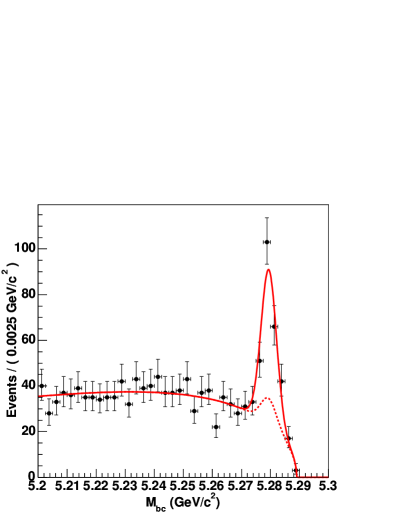
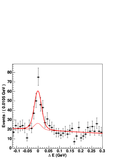
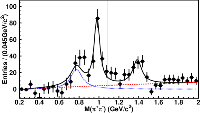
Figure 8: Distributions of (a) ${M_{\rm bc}}$ in the ${\Delta E}$ signal region, (b) ${\Delta E}$ in the ${M_{\rm bc}}$ signal region and (c) $m_{{\pi^{+}}{\pi^{-}}}$ in the ${\Delta E}$-${M_{\rm bc}}$ signal region for ${B^{0}}\to{f_{0}}{K_{S}^{0}}$ candidates. Solid curves show the fits to signal plus background distributions. Dashed curves in (a) and (b) show the background contributions. In (c), each point shows a yield for ${B^{0}}\to{\pi^{+}}{\pi^{-}}{K_{S}^{0}}$ including ${f_{0}}{K_{S}^{0}}$ obtained from a fit to the ${\Delta E}$-${M_{\rm bc}}$ distribution, the dotted line shows the ${B^{0}}\to\rho{K_{S}^{0}}$, and the dashed line shows other quasi two-body decays as well as three-body ${B^{0}}\to{\pi^{+}}{\pi^{-}}{K_{S}^{0}}$ decays.

For the signal yield extraction, we first perform an unbinned two-dimensional maximum-likelihood fit to the ${\Delta E}$-${M_{\rm bc}}$ distribution in the fit region defined as ${M_{\rm bc}}>5.2~{}{\rm GeV/}c^{2}$ and $-0.12~{}{\rm GeV}<{\Delta E}<0.3~{}{\rm GeV}$. The signal is modeled with a Gaussian function (a sum of two Gaussian functions) for ${M_{\rm bc}}$ (${\Delta E}$). For the continuum background, we use the ARGUS parameterization for ${M_{\rm bc}}$ and a linear function for ${\Delta E}$. The fit yields the number of ${B^{0}}\to{\pi^{+}}{\pi^{-}}{K_{S}^{0}}$ events that have ${\pi^{+}}{\pi^{-}}$ invariant masses within the ${f_{0}}$ resonance region, which may include contributions from ${B^{0}}\to{\rho^{0}}{K_{S}^{0}}$ as well as non-resonant three-body ${B^{0}}\to{\pi^{+}}{\pi^{-}}{K_{S}^{0}}$ decays. To separate these peaking backgrounds from the ${B^{0}}\to{f_{0}}{K_{S}^{0}}$ decay, we perform another fit to the ${\pi^{+}}{\pi^{-}}$ invariant mass distribution for the events inside the ${\Delta E}$-${M_{\rm bc}}$ signal region. We use Breit-Wigner functions for the ${B^{0}}\to{f_{0}}{K_{S}^{0}}$ signal, for the ${B^{0}}\to\rho{K_{S}^{0}}$ background and for a possible resonance above the ${f_{0}}$ mass region, which is referred to as ${f_{X}(1300)}$. The contributions from other resonant or non-resonant ${B^{0}}\to{\pi^{+}}{\pi^{-}}{K_{S}^{0}}$ decays are modeled with a threshold function. The combinatorial background is represented by the ${M_{\rm bc}}$-${\Delta E}$ sideband and subtracted from the signal region distribution. The ${\pi^{+}}{\pi^{-}}$ invariant mass distribution with the fit result is shown in Fig. 8(c). The fit yields $145\pm 16$ ${B^{0}}\to{f_{0}}{K_{S}^{0}}$ events.

II.9 ${B^{0}}\to\omega{K_{S}^{0}}$

Candidate ${K_{S}^{0}}\to{\pi^{+}}{\pi^{-}}$ decays are selected with criteria that are identical to those used for the ${B^{0}}\to\phi{K_{S}^{0}}$ decay. Pions for the $\omega\to{\pi^{+}}{\pi^{-}}{\pi^{0}}$ decay are selected with the same criteria used for the $\eta\to{\pi^{+}}{\pi^{-}}{\pi^{0}}$ decay, except that we require $p_{\pi^{0}}^{\rm cms}>0.35~{}{\rm GeV}/c$. The ${\pi^{+}}{\pi^{-}}{\pi^{0}}$ invariant mass $M_{3\pi}$ is required to be between 0.73 GeV/$c^{2}$ and 0.84 GeV/$c^{2}$. The $B$ meson signal region is defined as $-0.10~{}{\rm GeV}<{\Delta E}<0.08~{}{\rm GeV}$ and $5.27~{}{\rm GeV}/c^{2}<{M_{\rm bc}}<5.29~{}{\rm GeV}/c^{2}$. The ${\Delta E}$ resolution is 0.028 GeV. The dominant background is from continuum. The continuum suppression is based on the likelihood ratio ${\cal R}_{\rm s/b}$ obtained from the same discriminating variables used for the ${B^{0}}\to\phi{K_{S}^{0}}$ decay plus the helicity angle $\theta_{H}$ defined as the angle between the ${B^{0}}$ meson momentum and the cross product of the ${\pi^{+}}$ and ${\pi^{-}}$ momenta in the $\omega$ meson rest frame. We also require $|\cos\theta_{T}|<0.9$ prior to the ${\cal R}_{\rm s/b}$ requirement. We define two ${\cal R}_{\rm s/b}$ regions. The ${\cal R}_{\rm s/b}$ requirements depend on the flavor-tagging quality. The boundary between the high-${\cal R}_{\rm s/b}$ regions and the low-${\cal R}_{\rm s/b}$ regions is 0.85 for all $r$ values. The minimum ${\cal R}_{\rm s/b}$ requirements range from 0.1 to 0.6 for the low-${\cal R}_{\rm s/b}$ regions. The ${\cal R}_{\rm s/b}$ and $|\cos\theta_{T}|$ requirements reject 85% of the continuum background while retaining 84% of the signal. The contribution from $B\overline{B}$ events is negligibly small.

Figures 9(a-c) show the ${M_{\rm bc}}$ distribution for the reconstructed ${B^{0}}\to\omega{K_{S}^{0}}$ candidates within the ${\Delta E}$ signal region, the ${\Delta E}$ distribution within the ${M_{\rm bc}}$ signal region and the $M_{3\pi}$ distribution within the ${\Delta E}$-${M_{\rm bc}}$ signal region, respectively, after flavor tagging and vertex reconstruction.

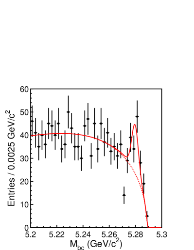
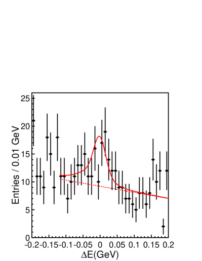
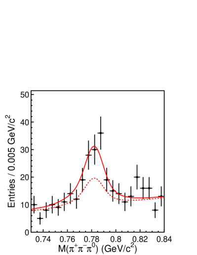
Figure 9: Distributions of (a) ${M_{\rm bc}}$ within the ${\Delta E}$ signal region, (b) ${\Delta E}$ within the ${M_{\rm bc}}$ signal region and (c) $m_{{\pi^{+}}{\pi^{-}}{\pi^{0}}}$ within the ${\Delta E}$-${M_{\rm bc}}$ signal region for ${B^{0}}\to\omega{K_{S}^{0}}$ candidates. Solid curves show the fits to signal plus background distributions, and dashed curves show the background contributions.

The signal yield is determined from an unbinned three-dimensional maximum-likelihood fit to the ${\Delta E}$-${M_{\rm bc}}$-$M_{3\pi}$ distribution in the fit region defined as ${M_{\rm bc}}>5.2~{}{\rm GeV/}c^{2}$, $-0.12~{}{\rm GeV}<{\Delta E}<0.25~{}{\rm GeV}$ and $0.73~{}{\rm GeV}/c^{2}<M_{3\pi}<0.84~{}{\rm GeV}/c^{2}$. The ${B^{0}}\to\omega{K_{S}^{0}}$ signal distribution is modeled with a sum of two (three) Gaussian functions for ${M_{\rm bc}}$ (${\Delta E}$ and $M_{3\pi}$). For the continuum background, we use the ARGUS parameterization for ${M_{\rm bc}}$, a linear function for ${\Delta E}$ and a second-order polynomial function plus three Gaussian functions for $M_{3\pi}$. The fit yields $68\pm 13$ ${B^{0}}\to\omega{K_{S}^{0}}$ events in the signal region.

II.10 ${B^{0}}\to{J/\psi}{K_{S}^{0}}$ and ${J/\psi}{K_{L}^{0}}$

The reconstruction and selection criteria for ${B^{0}}\to{J/\psi}{K_{S}^{0}}$ decays used in this measurement are the same as those in the previous publication, which are described in detail elsewhere bib:CP1_Belle . We reconstruct ${J/\psi}$ candidates via their decays to $\ell^{+}\ell^{-}$ ($\ell=\mu,e$), and ${K_{S}^{0}}$ candidates via ${K_{S}^{0}}\to{\pi^{+}}{\pi^{-}}$ decays. The $B$ meson signal region is defined as $|{\Delta E}|<0.04$ GeV and $5.27~{}{\rm GeV}/c^{2}<{M_{\rm bc}}<5.29~{}{\rm GeV}/c^{2}$.

Candidate ${J/\psi}\to\mu^{+}\mu^{-}$ or $e^{+}e^{-}$ decays for the ${B^{0}}\to{J/\psi}{K_{L}^{0}}$ mode are selected by requiring 3.05 GeV/$c^{2}<M_{\mu\mu}<3.13$ GeV/$c^{2}$ or 2.95 GeV/$c^{2}<M_{ee}<3.13$ GeV/$c^{2}$, where $M_{\mu\mu}~{}(M_{ee})$ is the invariant mass of the $\mu^{+}\mu^{-}$ $(e^{+}e^{-})$ pair. The momentum of the reconstructed ${J/\psi}$ candidate is required to be between 1.38 GeV/$c$ and 2.00 GeV/$c$. The selection criteria for ${K_{L}^{0}}$ candidates are identical to those in the ${B^{0}}\to\phi{K_{L}^{0}}$ analysis, except that the ${K_{L}^{0}}$ likelihood ratio for the ECL cluster is required to be greater than 0.25 for both KLM+ECL and ECL candidates. The $B$ signal region is defined as $0.2~{}{\rm GeV}/c<p_{B}^{\rm cms}<0.45~{}{\rm GeV}/c$.

Figure 10(a) shows the ${M_{\rm bc}}$ distribution for the reconstructed ${B^{0}}\to{J/\psi}{K_{S}^{0}}$ candidates within the ${\Delta E}$ signal region after flavor tagging and vertex reconstruction. The ${\Delta E}$ distribution for the ${B^{0}}\to{J/\psi}{K_{S}^{0}}$ candidates within the ${M_{\rm bc}}$ signal region is shown in Fig. 10(b). The signal yield for the ${B^{0}}\to{J/\psi}{K_{S}^{0}}$ decay is determined from an unbinned two-dimensional maximum-likelihood fit to the ${\Delta E}$-${M_{\rm bc}}$ distribution. The fit region is defined as $|{\Delta E}|<0.05~{}{\rm GeV}$ and ${M_{\rm bc}}>5.2~{}{\rm GeV/}c^{2}$. The signal distribution is modeled with a Gaussian function (a sum of two Gaussian functions) for ${M_{\rm bc}}$ (${\Delta E}$). For the background, we use the ARGUS parameterization for ${M_{\rm bc}}$ and a linear function for ${\Delta E}$. Figure 10(c) shows the $p_{B}^{\rm cms}$ distribution for the reconstructed ${B^{0}}\to{J/\psi}{K_{L}^{0}}$ candidates. The signal yield for the ${B^{0}}\to{J/\psi}{K_{L}^{0}}$ decay is determined from a binned maximum-likelihood fit to the $p_{B}^{\rm cms}$ distribution for each of KLM, KLM+ECL and ECL candidates separately. The fit region is defined as $0~{}{\rm GeV}/c<p_{B}^{\rm cms}<2~{}{\rm GeV}/c$. The shapes of the signal and background with $J/\psi$ are determined from the $J/\psi$ inclusive MC sample. Here background distributions with ${K_{L}^{0}}$ and without ${K_{L}^{0}}$ are treated separately to minimize the effect of an uncertainty in the ${K_{L}^{0}}$ detection efficiency in the MC simulation. The background shape for the case with a fake $J/\psi$ meson is obtained from events in the sideband of the $\ell^{+}\ell^{-}$ mass distribution.

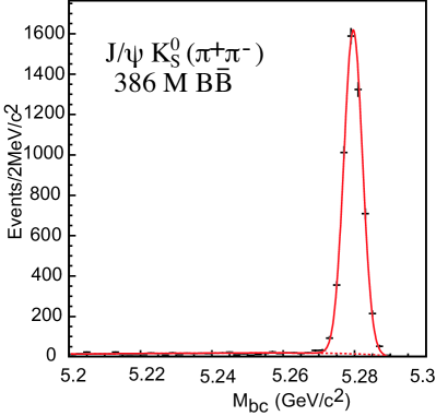
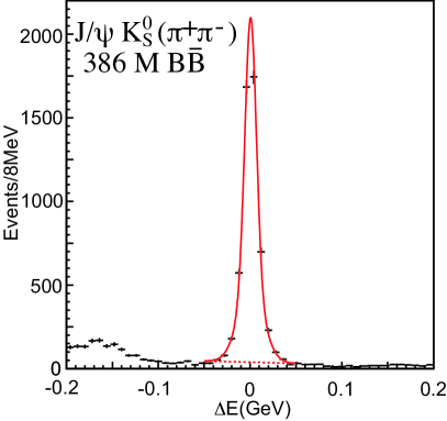
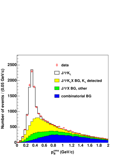
Figure 10: Distributions of (a) ${M_{\rm bc}}$ within the ${\Delta E}$ signal region and (b) ${\Delta E}$ within the ${M_{\rm bc}}$ signal region for ${B^{0}}\to{J/\psi}{K_{S}^{0}}$ candidates, and (c) $p_{B}^{\rm cms}$ for ${B^{0}}\to{J/\psi}{K_{L}^{0}}$ candidates.

II.11 Flavor Tagging

The $b$-flavor of the accompanying $B$ meson is identified from inclusive properties of particles that are not associated with the reconstructed ${B^{0}}\to f_{CP}$ decay. We use the same procedure as for our previous ${\sin 2\phi_{1}}$ measurement bib:BELLE-CONF-0436 . The algorithm for flavor tagging is described in detail elsewhere bib:fbtg_nim . We use two parameters, $q$ and $r$, to represent the tagging information. The first, $q$, is defined in Eq. (1). The parameter $r$ is an event-by-event, MC-determined flavor-tagging dilution factor that ranges from $r=0$ for no flavor discrimination to $r=1$ for unambiguous flavor assignment. It is used only to sort data into six $r$ intervals listed in Table 1. The wrong tag fractions for the six $r$ intervals, $w_{l}~{}(l=1,6)$, and differences between ${B^{0}}$ and ${\overline{B}{}^{0}}$ decays, ${\Delta w_{l}}$, are determined from the data; we use the same values that were used for the $\sin 2\phi_{1}$ measurement bib:BELLE-CONF-0436 for DS-I. Wrong tag fractions for DS-II are separately obtained with the same procedure and are listed in Table 1.

Table 1: Event fractions $\epsilon_{l}$, wrong-tag fractions $w_{l}$, wrong-tag fraction differences ${\Delta w_{l}}$, and average effective tagging efficiencies $\epsilon_{\textrm{eff}}^{l}=\epsilon_{l}(1-2w_{l})^{2}$ for each $r$ interval for DS-II. Errors for $w_{l}$ and ${\Delta w_{l}}$ include both statistical and systematic uncertainties. The event fractions are obtained from ${J/\psi}{K_{S}^{0}}$ data.

$l$	$r$ interval	$\epsilon_{l}$	$w_{l}$	${\Delta w_{l}}$	$\epsilon_{\textrm{eff}}^{l}$
1	0.000 – 0.250	$0.384\pm 0.011$	$0.467\pm 0.006$	$+0.005\pm 0.007$	$0.002\pm 0.001$
2	0.250 – 0.500	$0.165\pm 0.007$	$0.324\pm 0.007$	$-0.029\pm 0.009$	$0.021\pm 0.002$
3	0.500 – 0.625	$0.105\pm 0.006$	$0.223\pm 0.010$	$+0.019\pm 0.011$	$0.032\pm 0.003$
4	0.625 – 0.750	$0.112\pm 0.006$	$0.160\pm 0.011$	$+0.008\pm 0.011$	$0.052\pm 0.004$
5	0.750 – 0.875	$0.089\pm 0.005$	$0.101\pm 0.009$	$-0.022\pm 0.010$	$0.057\pm 0.004$
6	0.875 – 1.000	$0.144\pm 0.007$	$0.020\pm 0.006$	$+0.003\pm 0.006$	$0.133\pm 0.007$

The total effective tagging efficiency for DS-II is determined to be $\epsilon_{\textrm{eff}}\equiv\sum_{l=1}^{6}\epsilon_{l}(1-2w_{l})^{2}={0.30\pm 0.01}$, where $\epsilon_{l}$ is the event fraction for each $r$ interval determined from the ${J/\psi}{K_{S}^{0}}$ data and is listed in Table 1. The error includes both statistical and systematic uncertainties. We find that the wrong tag fractions for DS-II are slightly smaller than those for DS-I. As a result, the $\epsilon_{\textrm{eff}}$ value for DS-II is slightly larger than that for DS-I ($\epsilon_{\textrm{eff}}={0.287\pm 0.005}$).

II.12 Vertex Reconstruction

The vertex position for the $f_{CP}$ decay is reconstructed using charged tracks that have enough SVD hits: at least one layer with hits on both sides and at least one additional $z$ hit in other layers for SVD-I, and at least two layers with hits on both sides for SVD-II. A constraint on the IP is also used with the selected tracks; the IP profile is convolved with the finite $B$ flight length in the plane perpendicular to the $z$ axis. The pions from ${K_{S}^{0}}$ decays are not used except in the analysis of ${B^{0}}\to{K_{S}^{0}}{\pi^{0}}$ and ${K_{S}^{0}}{K_{S}^{0}}{K_{S}^{0}}$ decays. The typical vertex reconstruction efficiency and $z$ resolution for ${B^{0}}\to\phi{K_{S}^{0}}$ decays are 95% and 78 $\mu$m, respectively. Similar values are obtained for other $f_{CP}$ decays except for ${B^{0}}\to{K_{S}^{0}}{\pi^{0}}$ and ${K_{S}^{0}}{K_{S}^{0}}{K_{S}^{0}}$ decays.

The vertex for ${B^{0}}\to{K_{S}^{0}}{\pi^{0}}$ decays is reconstructed using the ${K_{S}^{0}}$ trajectory and the IP constraint, where both pions from the ${K_{S}^{0}}$ decay are required to have enough SVD hits in the same way as for other $f_{CP}$ decays. The reconstruction efficiency depends both on the ${K_{S}^{0}}$ momentum and on the SVD geometry; the efficiency with SVD-II (32%) is significantly higher than that with SVD-I (23%) because of the larger outer radius and the additional layer. The typical $z$ resolution of the vertex reconstructed with the ${K_{S}^{0}}$ is 93 $\mu$m for SVD-I and 110 $\mu$m for SVD-II.

The vertex position for ${B^{0}}\to{K_{S}^{0}}{K_{S}^{0}}{K_{S}^{0}}$ decays is also obtained using ${K_{S}^{+-}}$ trajectories and a constraint on the IP. The reconstruction efficiency depends both on the ${K_{S}^{+-}}$ momentum and on the SVD geometry. The vertex efficiencies with SVD-I (SVD-II) are 79% (86%) for ${K_{S}^{+-}}{K_{S}^{+-}}{K_{S}^{+-}}$ and 62% (74%) for ${K_{S}^{+-}}{K_{S}^{+-}}{K_{S}^{00}}$. The typical vertex resolution is about 97 $\mu$m (113 $\mu$m) for SVD-I (SVD-II) when two or three ${K_{S}^{+-}}$ candidates can be used. The resolution is worse when only one ${K_{S}^{+-}}$ can be used; the typical value is 152 $\mu$m (168 $\mu$m) for SVD-I (SVD-II), which is comparable to the $f_{\rm tag}$ vertex resolution.

The $f_{\rm tag}$ vertex determination with SVD-I remains unchanged from the previous publication Chen:2005dr , and is described in detail elsewhere bib:resol_nim ; to minimize the effect of long-lived particles, secondary vertices from charmed hadrons and a small fraction of poorly reconstructed tracks, we adopt an iterative procedure in which the track that gives the largest contribution to the vertex $\chi^{2}$ is removed at each step until a good $\chi^{2}$ is obtained. The reconstruction efficiency was measured to be 93%. The typical $z$ resolution is $140~{}\mu$m bib:CP1_Belle .

For SVD-II, we find that the same vertex reconstruction algorithm results in a larger outlier fraction when only one track remains after the iteration procedure. Therefore, in this case, we repeat the iteration procedure with a more stringent requirement on the SVD-II hit pattern; at least two of the three outer layers have hits on both sides. The resulting outlier fraction, which is described in Sec. III, is comparable to that for SVD-I, while the inefficiency caused by this change is small (2.5%).

II.13 Summary of Signal Yields

The signal yields that contribute to the determination of $CP$-violation parameters, ${N_{\rm sig}}$, for ${B^{0}}\to f_{CP}$ decays are summarized in Table 2. These yields are obtained after flavor tagging and vertex reconstruction for all modes except ${B^{0}}\to{K_{S}^{0}}{\pi^{0}}$. As events with no vertex information reduce the statistical error on ${\cal A}_{{K_{S}^{0}}{\pi^{0}}}$ significantly, we include them in the fit for the ${B^{0}}\to{K_{S}^{0}}{\pi^{0}}$ decay. The signal purities are also listed in the table. The signal yields are all consistent with expected values that are obtained from previously measured branching fractions bib:HFAG and reconstruction efficiencies estimated from MC simulation studies.

Table 2: Estimated signal purities and signal yields ${N_{\rm sig}}$ in the signal region for each $f_{CP}$ mode that is used to measure $CP$ asymmetries. The purity is defined as ${N_{\rm sig}}/{N_{\rm ev}}$, where ${N_{\rm ev}}$ is the total number of events in the signal region. Results for ${B^{0}}\to{K_{S}^{0}}{\pi^{0}}$ decays are obtained with samples after flavor tagging but before vertex reconstruction. Results for other decays are obtained after flavor tagging and vertex reconstruction.

Mode		$\xi_{f}$	purity	${N_{\rm sig}}$
$\phi{K_{S}^{0}}$		$-1$	$0.57$	$180\pm 16$
$\phi{K_{L}^{0}}$		$+1$	$0.12$	$78\pm 13$
$\eta^{\prime}{K_{S}^{0}}$		$-1$	$0.61$	$830\pm 35$
$\eta^{\prime}{K_{L}^{0}}$		$+1$	$0.26$	$187\pm 18$
${K_{S}^{0}}{K_{S}^{0}}{K_{S}^{0}}$		$+1$	$0.64$	$105\pm 12$
${K_{S}^{0}}{\pi^{0}}$		$-1$	$0.25$	$344\pm 30$
${f_{0}}{K_{S}^{0}}$		$+1$	$0.47$	$145\pm 16$
$\omega{K_{S}^{0}}$		$-1$	$0.17$	$68\pm 13$
${K^{+}}{K^{-}}{K_{S}^{0}}$		$+0.86\pm 0.18\pm 0.09$	$0.55$	$536\pm 29$
${J/\psi}{K_{S}^{0}}$		$-1$	$0.98$	$5264\pm 73$
${J/\psi}{K_{L}^{0}}$		$+1$	$0.60$	$4792\pm 105$

III Results of $CP$ Asymmetry Measurements

We determine ${\cal S}_{f}$ and ${\cal A}_{f}$ for each mode by performing an unbinned maximum-likelihood fit to the observed $\Delta t$ distribution. The probability density function (PDF) expected for the signal distribution, ${\cal P}_{\rm sig}(\Delta t;{\cal S}_{f},{\cal A}_{f},q,w_{l},{\Delta w_{l}})$, is given by Eq. (1) incorporating the effect of incorrect flavor assignment. The distribution is convolved with the proper-time interval resolution function ${R_{\rm sig}(\Delta t)}$, which takes into account the finite vertex resolution.

For the decays ${B^{0}}\to$ $\phi{K_{S}^{0}}$, $\phi{K_{L}^{0}}$, $\eta^{\prime}{K_{S}^{0}}$, ${\eta^{\prime}}{K_{L}^{0}}$, ${f_{0}}{K_{S}^{0}}$, $\omega{K_{S}^{0}}$, ${K^{+}}{K^{-}}{K_{S}^{0}}$, ${J/\psi}{K_{S}^{0}}$ and ${J/\psi}{K_{L}^{0}}$, we use flavor-specific $B$ decays governed by semileptonic or hadronic $b\to c$ transitions to determine the resolution function. We perform a simultaneous multiparameter fit to these high-statistics control samples to obtain the resolution function parameters, wrong-tag fractions (Section II.11), $\Delta m_{d}$, ${\tau_{B^{+}}}$ and ${\tau_{B^{0}}}$. We use the same resolution function used for the ${\sin 2\phi_{1}}$ measurement for DS-I bib:BELLE-CONF-0436 . For DS-II, the following modifications are introduced: a sum of two Gaussian functions is used to model the resolution of the $f_{CP}$ vertex while a single Gaussian function is used for DS-I; a sum of two Gaussian functions is used to model the resolution of the tag-side vertex obtained with one track and the IP constraint, while a single Gaussian function is used for DS-I. These modifications are needed to account for differences between SVD-I and SVD-II, as well as different background conditions in DS-I and DS-II. We test the resolution parameterization using MC events on which we overlay beam-related background taken from data. A fit to the MC sample yields correct values for all parameters.

For the ${B^{0}}\to{K_{S}^{0}}{\pi^{0}}$ decay, we use the resolution function described above with additional parameters that rescale vertex errors. The rescaling function depends on the detector configuration (SVD-I or SVD-II), SVD hit patterns of charged pions from the ${K_{S}^{0}}$ decay, and ${K_{S}^{0}}$ decay vertex position in the plane perpendicular to the beam axis. The parameters in the rescaling function are determined from a fit to the $\Delta t$ distribution of ${B^{0}}\to{J/\psi}{K_{S}^{0}}$ data. Here only the ${K_{S}^{0}}$ and the IP constraint are used for the vertex reconstruction, the ${B^{0}}$ lifetime is fixed at the world average value, and $b$-flavor tagging information is not used so that the expected PDF is an exponential function convolved with the resolution function.

We check the resulting resolution function by also reconstructing the vertex with leptons from ${J/\psi}$ decays and the IP constraint. We find that the distribution of the distance between the vertex positions obtained with the two methods is well represented by the resolution function convolved with the well-known resolution for the ${J/\psi}$ vertex. Finally, we also perform a fit to the ${B^{0}}\to{J/\psi}{K_{S}^{0}}$ sample with $b$-flavor information and obtain ${\cal S}_{{J/\psi}{K_{S}^{0}}}=+0.73\pm 0.08$(stat) and ${\cal A}_{{J/\psi}{K_{S}^{0}}}=+0.01\pm 0.04$(stat), which are in good agreement with our measurement using leptons from ${J/\psi}$ decays, which will be described later. A separate fit to the same sample with ${\tau_{B^{0}}}$ as a free parameter yields ${\tau_{B^{0}}}=1.55\pm 0.05$(stat) ps, which is consistent with the world average value. Thus, we conclude that the vertex resolution for the ${B^{0}}\to{K_{S}^{0}}{\pi^{0}}$ decay is well understood.

For ${B^{0}}\to{K_{S}^{0}}{K_{S}^{0}}{K_{S}^{0}}$ candidates, we use the same resolution function that is used for the ${B^{0}}\to{K_{S}^{0}}{\pi^{0}}$ decay if only one ${K_{S}^{+-}}$ is available for the vertex reconstruction. For events with $n$ (= 2 or 3) ${K_{S}^{+-}}$ trajectories used in the vertexing, we adopt a function defined as $[{\cal V}(\sigma_{z})]^{1/n}$ to rescale the vertex error $\sigma_{z}$. Here ${\cal V}(\sigma_{z})$ is the aforementioned rescaling function for the case that only one ${K_{S}^{+-}}$ is available. We find from MC simulation that the resolution is well described by this form for the rescaling function.

We determine the following likelihood for each event:

$$P_{i} = (1-f_{\rm ol})\int\biggl{[}f_{\rm sig}{\cal P}_{\rm sig}(\Delta t^{\prime})R_{\rm sig}(\Delta t_{i}-\Delta t^{\prime})$$ (2)

$$+ (1-f_{\rm sig}){\cal P}_{\rm bkg}(\Delta t^{\prime})R_{\rm bkg}(\Delta t_{i}-\Delta t^{\prime})\biggr{]}d(\Delta t^{\prime})$$

$$+ f_{\rm ol}P_{\rm ol}(\Delta t_{i}),$$

where $P_{\rm ol}(\Delta t)$ is a broad Gaussian function that represents an outlier component with a small fraction $f_{\rm ol}$ bib:BELLE-CONF-0436 . The width of the outlier component for DS-I is determined to be $(39^{+2}_{-13})$ ps; the fractions of the outlier components are $(2.1^{+1.2}_{-0.8})\times 10^{-4}$ for events with the $f_{\rm tag}$ vertex reconstructed with more than one track, and $(3.1^{+0.3}_{-0.6})\times 10^{-2}$ for the case only one track is used. Here the errors include both statistical and systematic errors. Corresponding values for DS-II are $(35^{+8}_{-11})$ ps, $(3.6^{+2.0}_{-1.1})\times 10^{-4}$ and $(1.8^{+0.2}_{-0.3})\times 10^{-2}$. The signal probability $f_{\rm sig}$ depends on the $r$ region and is calculated on an event-by-event basis as a function of $p_{B}^{\rm cms}$ for the ${B^{0}}\to{J/\psi}{K_{L}^{0}}$ decay, $p_{B}^{\rm cms}$ and ${\cal R}_{\rm s/b}$ for the ${B^{0}}\to\phi{K_{L}^{0}}$ and ${\eta^{\prime}}{K_{L}^{0}}$ decays, ${\Delta E}$, ${M_{\rm bc}}$ and $\cos\theta_{H}$ for the ${B^{0}}\to\phi{K_{S}^{0}}$ decay, ${\Delta E}$, ${M_{\rm bc}}$ and $M_{3\pi}$ for the $\omega{K_{S}^{0}}$ decays, and ${\Delta E}$ and ${M_{\rm bc}}$ for the other modes. A PDF for background events, ${\cal P}_{\rm bkg}(\Delta t)$, is modeled as a sum of exponential and prompt components, and is convolved with a sum of two Gaussians $R_{\rm bkg}$. Parameters in ${\cal P}_{\rm bkg}(\Delta t)$ and $R_{\rm bkg}$ for continuum background are determined by a fit to the $\Delta t$ distribution for events outside the ${\Delta E}$-${M_{\rm bc}}$ signal region except for the ${B^{0}}\to\phi{K_{L}^{0}}$ and ${\eta^{\prime}}{K_{L}^{0}}$ decays. For the ${B^{0}}\to\phi{K_{L}^{0}}$ and ${\eta^{\prime}}{K_{L}^{0}}$ decays, we use $p_{B}^{\rm cms}$ sideband events to obtain the parameters. Parameters in ${\cal P}_{\rm bkg}(\Delta t)$ and $R_{\rm bkg}$ for $B\overline{B}$ background events in ${B^{0}}\to\eta^{\prime}{K_{S}^{0}}$, ${K_{S}^{0}}{\pi^{0}}$, $\phi{K_{L}^{0}}$ and ${\eta^{\prime}}{K_{L}^{0}}$ decays are determined from MC simulation.

We fix $\tau_{B^{0}}$ and $\Delta m_{d}$ at their world average values bib:PDG2005 . We assume no $CP$ asymmetry in the background $\Delta t$ distributions and possible $CP$ asymmetries in the $B$ decay backgrounds are treated as sources of systematic error. In order to reduce the statistical error on ${\cal A}_{f}$, we include events without vertex information in the analysis of ${B^{0}}\to{K_{S}^{0}}{\pi^{0}}$. The likelihood in this case is obtained by integrating Eq. (2) over $\Delta t_{i}$.

The only free parameters in the final fits are ${\cal S}_{f}$ and ${\cal A}_{f}$, which are determined by maximizing the likelihood function $L=\prod_{i}P_{i}(\Delta t_{i};{\cal S}_{f},{\cal A}_{f})$ where the product is over all events. Table 3 summarizes the fit results of ${\cal S}_{f}$ and ${\cal A}_{f}$. We define the raw asymmetry in each $\Delta t$ bin by $(N_{q=+1}-N_{q=-1})/(N_{q=+1}+N_{q=-1})$, where $N_{q=+1(-1)}$ is the number of observed candidates with $q=+1(-1)$. Figures 11-14 show the raw asymmetries for each decay mode in two regions of the flavor-tagging parameter $r$ footnote:rawasym .

Table 3: Results of the fits to the $\Delta t$ distributions. The first error is statistical and the second error is systematic.

Mode	SM expectation for ${\cal S}_{f}$	${\cal S}_{f}$	${\cal A}_{f}$
$\phi{K^{0}}$	$+{\sin 2\phi_{1}}$	$+0.44\pm 0.27\pm 0.05$	$+0.14\pm 0.17\pm 0.07$
$\phi{K_{S}^{0}}$	$+{\sin 2\phi_{1}}$	$+0.19\pm 0.32$	$+0.12\pm 0.20$
$\phi{K_{L}^{0}}$	$-{\sin 2\phi_{1}}$	$-1.54\pm 0.59$	$+0.38\pm 0.36$
$\eta^{\prime}{K^{0}}$	$+{\sin 2\phi_{1}}$	$+0.62\pm 0.12\pm 0.04$	$-0.04\pm 0.08\pm 0.06$
${\eta^{\prime}}{K_{S}^{0}}$	$+{\sin 2\phi_{1}}$	$+0.60\pm 0.14$	$-0.04\pm 0.09$
${\eta^{\prime}}{K_{L}^{0}}$	$-{\sin 2\phi_{1}}$	$-0.73\pm 0.29$	$-0.02\pm 0.18$
${K_{S}^{0}}{K_{S}^{0}}{K_{S}^{0}}$	$-{\sin 2\phi_{1}}$	$-0.58\pm 0.36\pm 0.08$	$+0.50\pm 0.23\pm 0.06$
${K_{S}^{0}}{\pi^{0}}$	$+{\sin 2\phi_{1}}$	$+0.22\pm 0.47\pm 0.08$	$+0.11\pm 0.18\pm 0.08$
${f_{0}}{K_{S}^{0}}$	$-{\sin 2\phi_{1}}$	$-0.47\pm 0.36\pm 0.08$	$-0.23\pm 0.23\pm 0.13$
$\omega{K_{S}^{0}}$	$+{\sin 2\phi_{1}}$	$+0.95\pm 0.53^{+0.12}_{-0.15}$	$+0.19\pm 0.39\pm 0.13$
${K^{+}}{K^{-}}{K_{S}^{0}}$	$-(2f_{+}-1){\sin 2\phi_{1}}$	$-0.52\pm 0.16\pm 0.03$	$-0.06\pm 0.11\pm 0.07$
${J/\psi}{K^{0}}$	$+{\sin 2\phi_{1}}$	$+0.652\pm 0.039\pm 0.020$	$+0.010\pm 0.026\pm 0.036$
${J/\psi}{K_{S}^{0}}$	$+{\sin 2\phi_{1}}$	$+0.668\pm 0.047$	$-0.021\pm 0.034$
${J/\psi}{K_{L}^{0}}$	$-{\sin 2\phi_{1}}$	$-0.619\pm 0.069$	$+0.049\pm 0.039$

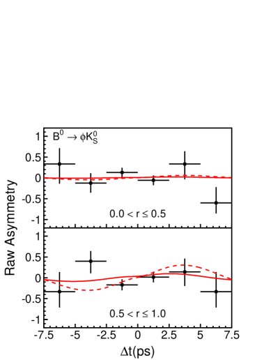
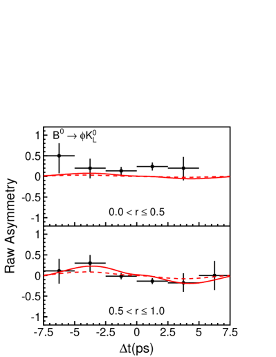
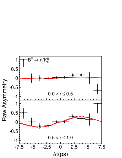
Figure 11: Raw asymmetry in each $\Delta t$ bin with $0<r\leq 0.5$ (top) and with $0.5<r\leq 1.0$ (bottom) for (a) ${B^{0}}\to\phi{K_{S}^{0}}$, (b) ${B^{0}}\to\phi{K_{L}^{0}}$, (c) ${B^{0}}\to\eta^{\prime}{K_{S}^{0}}$ and (d) ${B^{0}}\to\eta^{\prime}{K_{L}^{0}}$ decays. The solid curves show the results of the unbinned maximum-likelihood fits. The dashed curves show the SM expectation with our measurement of $CP$-violation parameters for the ${B^{0}}\to{J/\psi}{K^{0}}$ mode (${\sin 2\phi_{1}}=+0.652$ and ${\cal A}_{f}=+0.010$).

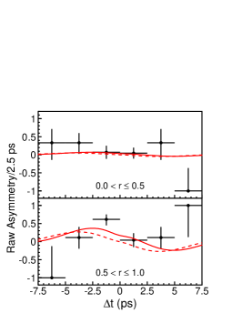
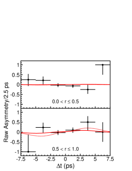
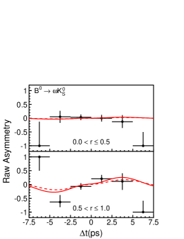
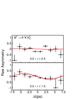
Figure 12: Raw asymmetry in each $\Delta t$ bin with $0<r\leq 0.5$ (top) and with $0.5<r\leq 1.0$ (bottom) for (a) ${B^{0}}\to{K_{S}^{0}}{K_{S}^{0}}{K_{S}^{0}}$ (b) ${B^{0}}\to{K_{S}^{0}}{\pi^{0}}$, (c) ${B^{0}}\to{f_{0}}{K_{S}^{0}}$, (d) ${B^{0}}\to\omega{K_{S}^{0}}$ and (e) ${B^{0}}\to{K^{+}}{K^{-}}{K_{S}^{0}}$ decays. The solid curves show the results of the unbinned maximum-likelihood fits. The dashed curves show the SM expectation with our measurement of $CP$-violation parameters for the ${B^{0}}\to{J/\psi}{K^{0}}$ mode (${\sin 2\phi_{1}}=+0.652$ and ${\cal A}_{f}=+0.010$).

Figure 13: $\Delta t$ distributions in (a) ${B^{0}}\to{J/\psi}{K_{S}^{0}}$, (b) ${B^{0}}\to{J/\psi}{K_{L}^{0}}$, and raw asymmetries in (c) ${B^{0}}\to{J/\psi}{K_{S}^{0}}$ and (d) ${B^{0}}\to{J/\psi}{K_{L}^{0}}$ with $0<r\leq 0.5$. The curves show the results of the unbinned maximum-likelihood fits.

Figure 14: $\Delta t$ distributions in (a) ${B^{0}}\to{J/\psi}{K_{S}^{0}}$, (b) ${B^{0}}\to{J/\psi}{K_{L}^{0}}$, and raw asymmetries in (c) ${B^{0}}\to{J/\psi}{K_{S}^{0}}$ and (d) ${B^{0}}\to{J/\psi}{K_{L}^{0}}$ with $0.5<r\leq 1$. The curves show the results of the unbinned maximum-likelihood fits.

Figures 15-17 also show $\Delta t$ distributions and asymmetries for ${B^{0}}\to\phi{K^{0}}$, ${\eta^{\prime}}{K^{0}}$ and ${J/\psi}{K^{0}}$ decays after subtracting background contributions, where the sign of each $\Delta t$ measurement for the final states with ${K_{L}^{0}}$ is inverted to combine final states with ${K_{S}^{0}}$ and ${K_{L}^{0}}$.

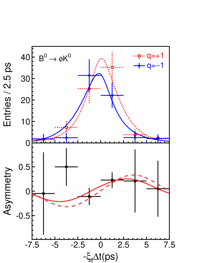
Figure 15: Background-subtracted $\Delta t$ distribution (top) and asymmetry in each $\Delta t$ bin (bottom) with $0.5<r\leq 1.0$ for ${B^{0}}\to\phi{K^{0}}$. The result of the unbinned maximum-likelihood fit is also shown. The dashed curve in the bottom figure shows the SM expectation with our measurement of $CP$-violation parameters for the ${B^{0}}\to{J/\psi}{K^{0}}$ mode (${\sin 2\phi_{1}}=+0.652$ and ${\cal A}_{f}=+0.010$).

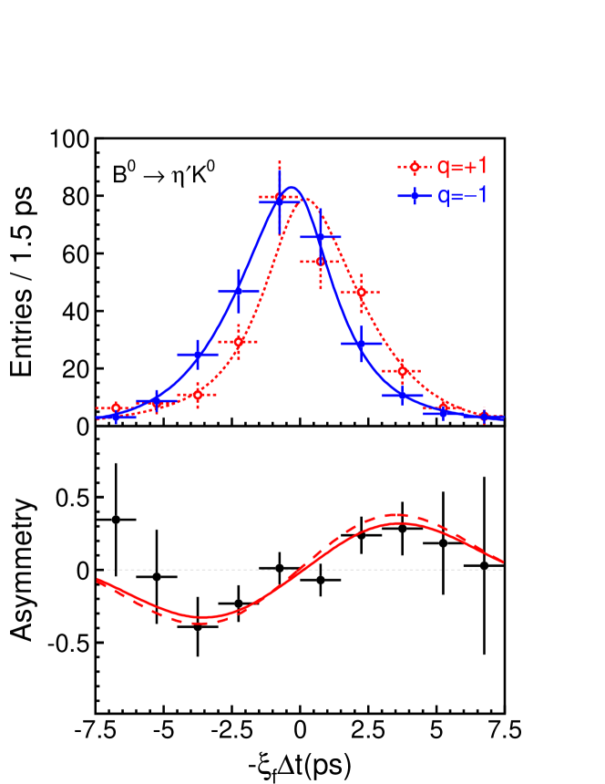
Figure 16: Background-subtracted $\Delta t$ distributions and asymmetry in each $\Delta t$ bin with $0.5<r\leq 1.0$ for ${B^{0}}\to\eta^{\prime}{K^{0}}$. The result of the unbinned maximum-likelihood fit is also shown. The dashed curve in the bottom figure shows the SM expectation with our measurement of $CP$-violation parameters for the ${B^{0}}\to{J/\psi}{K^{0}}$ mode (${\sin 2\phi_{1}}=+0.652$ and ${\cal A}_{f}=+0.010$).

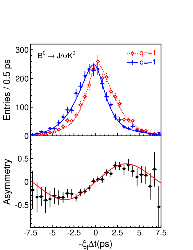
Figure 17: Background-subtracted $\Delta t$ distributions and asymmetry in each $\Delta t$ bin with $0.5<r\leq 1.0$ for ${B^{0}}\to{J/\psi}{K^{0}}$. The result of the unbinned maximum-likelihood fit is also shown.

Tables 4 and 5 list the systematic errors on ${\cal S}_{f}$ and ${\cal A}_{f}$, respectively. The total systematic errors are obtained by adding each contribution in quadrature, and are smaller than the statistical errors for all $b\to s$ modes.

To determine the systematic error that arises from uncertainties in the vertex reconstruction, the track and vertex selection criteria are varied to search for possible systematic biases. Small biases in the $\Delta z$ measurement are observed in $e^{+}e^{-}\to\mu^{+}\mu^{-}$ and other control samples. Systematic errors are estimated by applying special correction functions to account for the observed biases, repeating the fit, and comparing the obtained values with the nominal results. The systematic error due to the IP constraint in the vertex reconstruction is estimated by varying ($\pm 10\mu$m) the smearing used to account for the $B$ flight length. Systematic errors due to imperfect SVD alignment are determined from MC samples that have artificial misalignment effects to reproduce impact-parameter resolutions observed in data.

Systematic errors due to uncertainties in the wrong tag fractions are studied by varying the wrong tag fraction individually for each $r$ region. Systematic errors due to uncertainties in the resolution function are also estimated by varying each resolution parameter obtained from data (MC) by $\pm 1\sigma$ ($\pm 2\sigma$), repeating the fit and adding each variation in quadrature. Each physics parameter such as ${\tau_{B^{0}}}$ and $\Delta m_{d}$ is also varied by its error. A possible fit bias is examined by fitting a large number of MC events.

Systematic errors from uncertainties in the background fractions and in the background $\Delta t$ shape are estimated by varying each background parameter obtained from data (MC) by $\pm 1\sigma$ ($\pm 2\sigma$).

The PDF’s for ${B^{0}}\to\phi{K_{L}^{0}}$ and ${\eta^{\prime}}{K_{L}^{0}}$ assume no correlation among ${\cal R}_{\rm s/b}$, $p_{B}^{\rm cms}$ and $r$. To estimate systematic errors due to possible correlations between ${\cal R}_{\rm s/b}$ and $p_{B}^{\rm cms}$, we repeat a fit to obtain $CP$ parameters using signal fractions determined by the ${\cal R}_{\rm s/b}$ distribution for each $p_{B}^{\rm cms}$ region separately. The difference from our nominal result is included in the systematic error. Systematic errors due to other possible correlations are estimated from events in the $p_{B}^{\rm cms}$ sideband, events with $r<0.25$ and off-resonance data.

Additional sources of systematic errors are considered for $B$ decay backgrounds that are neglected in the PDF. We consider uncertainties both in their fractions and $CP$ asymmetries. The effect of backgrounds from ${K^{+}}{K^{-}}{K_{S}^{0}}$ and ${f_{0}}{K_{S}^{0}}~{}({f_{0}}\to{K^{+}}{K^{-}})$ in the ${B^{0}}\to\phi{K_{S}^{0}}$ sample is considered. Uncertainties from $B\to\phi K^{*}$ and other rare $B$ decay backgrounds in the ${B^{0}}\to\phi{K_{L}^{0}}$ sample are also taken into account. For the ${B^{0}}\to{\eta^{\prime}}{K_{S}^{0}}$ sample, non-resonant $B$ decay backgrounds are studied using events in the sideband of the reconstructed ${\eta^{\prime}}$ mass distribution. Effects of possible $CP$ asymmetries in $B$ decay backgrounds for ${K_{S}^{0}}{\pi^{0}}$ and ${f_{0}}{K_{S}^{0}}$ are evaluated. The peaking background fraction in the ${B^{0}}\to{f_{0}}{K_{S}^{0}}$ sample depends on the functions used to fit to the ${\pi^{+}}{\pi^{-}}$ invariant mass distribution. The systematic errors due to the uncertainties of the masses and widths of the resonances used in the fit are also included. The width of ${f_{0}}$ as well as the mass and the width of ${f_{X}(1300)}$ are varied by their errors. The effect of possible interference between resonant and non-resonant amplitudes, which is neglected in the nominal analysis, is also evaluated. We perform a fit to the ${\pi^{+}}{\pi^{-}}$ distribution of a MC sample generated with interfering amplitudes and phases for $B\to K\pi\pi$ decays measured from data Garmash:2003er . The observed difference in the signal yield from the true value is taken into account in the systematic error determination. We also repeat the fit to the $\Delta t$ distribution ignoring the contribution of the peaking background. The differences in ${\cal S}_{f}$ and ${\cal A}_{f}$ from our nominal results are included in the systematic error.

Finally, we investigate the effects of interference between CKM-favored and CKM-suppressed $B\to D$ transitions in the $f_{\rm tag}$ final state Long:2003wq . A small correction to the PDF for the signal distribution arises from the interference. We estimate the size of the correction using the ${B^{0}}\to D^{*-}\ell^{+}\nu$ sample. We then generate MC pseudoexperiments and make an ensemble test to obtain systematic biases in ${\cal S}_{f}$ and ${\cal A}_{f}$. In general, we find effects on ${\cal S}_{f}$ are negligibly small, while there are sizable possible shifts in ${\cal A}_{f}$.

Table 4: Summary of the systematic errors on ${\cal S}_{f}$.

	$\phi{K^{0}}$	$\eta^{\prime}{K^{0}}$	${K_{S}^{0}}{K_{S}^{0}}{K_{S}^{0}}$	${K_{S}^{0}}{\pi^{0}}$	${f_{0}}{K_{S}^{0}}$	$\omega{K_{S}^{0}}$	${K^{+}}{K^{-}}{K_{S}^{0}}$	${J/\psi}{K^{0}}$
Vertex reconstruction	$0.02$	$0.02$	$0.04$	$0.01$	$0.02$	$0.02$	$0.02$	$0.015$
Flavor tagging	$0.01$	$<0.01$	$0.01$	$0.01$	$0.01$	$0.04$	$<0.01$	$0.006$
Resolution function	$0.02$	$0.02$	$0.05$	$0.05$	$0.02$	$0.05$	$0.02$	$0.005$
Physics parameters	$<0.01$	$<0.01$	$<0.01$	$0.01$	$0.01$	$0.01$	$<0.01$	$0.001$
Possible fit bias	$0.01$	$0.02$	$0.03$	$0.01$	$0.02$	${}^{+0.01}_{-0.09}$	$0.01$	$0.007$
Background fraction	$0.01$	$0.02$	$0.02$	$0.01$	$0.02$	$0.09$	$0.02$	$0.005$
Background $\Delta t$ shape	$0.03$	$<0.01$	$0.02$	$0.06$	$0.07$	$0.01$	$0.01$	$0.006$
Tag-side interference	$<0.01$	$<0.01$	$0.01$	$<0.01$	$<0.01$	$<0.01$	$<0.01$	$0.003$
Total	$0.05$	$0.04$	$0.08$	$0.08$	$0.08$	${}^{+0.12}_{-0.15}$	$0.03$	$0.020$

Table 5: Summary of the systematic errors on ${\cal A}_{f}$.

	$\phi{K^{0}}$	$\eta^{\prime}{K^{0}}$	${K_{S}^{0}}{K_{S}^{0}}{K_{S}^{0}}$	${K_{S}^{0}}{\pi^{0}}$	${f_{0}}{K_{S}^{0}}$	$\omega{K_{S}^{0}}$	${K^{+}}{K^{-}}{K_{S}^{0}}$	${J/\psi}{K^{0}}$
Vertex reconstruction	$0.04$	$0.04$	$0.04$	$0.04$	$0.05$	$0.07$	$0.04$	$0.030$
Flavor tagging	$0.01$	$0.01$	$0.01$	$0.01$	$0.01$	$0.01$	$0.01$	$0.007$
Resolution function	$0.01$	$<0.01$	$0.02$	$<0.01$	$0.02$	$0.03$	$0.01$	$0.001$
Physics parameters	$<0.01$	$<0.01$	$<0.01$	$<0.01$	$<0.01$	$<0.01$	$<0.01$	$0.001$
Possible fit bias	$0.01$	$0.01$	$0.02$	$<0.01$	$0.01$	$0.02$	$0.01$	$0.005$
Background fraction	$0.01$	$0.01$	$0.03$	$0.01$	$0.01$	$0.10$	$0.01$	$0.004$
Background $\Delta t$ shape	$0.02$	$<0.01$	$0.01$	$0.03$	$0.09$	$0.01$	$<0.01$	$0.005$
Tag-side interference	$0.05$	$0.04$	$0.05$	$0.06$	$0.07$	$0.04$	$0.06$	$0.017$
Total	$0.07$	$0.06$	$0.06$	$0.08$	$0.13$	$0.13$	$0.07$	$0.036$

Various crosschecks of the measurements are performed. We reconstruct charged $B$ meson decays that are the counterparts of the ${B^{0}}\to f_{CP}$ decays and apply the same fit procedure. All results for the ${\cal S}_{f}$ term are consistent with no $CP$ asymmetry, as expected. Lifetime measurements are also performed for the $f_{CP}$ modes and the corresponding charged $B$ decay modes. The fits yield ${\tau_{B^{0}}}$ and ${\tau_{B^{+}}}$ values consistent with the world average values. MC pseudoexperiments are generated for each decay mode to perform ensemble tests. We find that the statistical errors obtained in our measurements are all consistent with the expectations from the ensemble tests.

The results in this report are consistent with those in our previous publications Chen:2005dr ; Sumisawa:2005fz ; bib:BELLE-CONF-0436 within statistical fluctuations and supersede them. Among our new results, the largest difference from the previous measurement is observed in the ${B^{0}}\to{K_{S}^{0}}{K_{S}^{0}}{K_{S}^{0}}$ decay. A fit to the $253$ fb^-1 data sample, which contains the entire DS-I and a part of DS-II and were used in the previous publication, yields ${\cal S}_{f}=+1.05\pm 0.64$(stat) and ${\cal A}_{f}=+0.51\pm 0.30$(stat), where a small change from the previous measurement is due to an improvement in the selection of ${K_{S}^{0}}$ candidates. A fit to an additional $104$ fb^-1 data sample alone yields ${\cal S}_{f}=-2.95\pm 0.53$(stat) and ${\cal A}_{f}=+0.64\pm 0.36$(stat). From MC pseudoexperiments, the probability that the significance of difference is larger than the observed difference is estimated to be 1.0%. To check if this arises due to a difference in the SVD1 and SVD2 detectors, we perform separate fits to DS-I and DS-II. We obtain ${\cal S}_{f}=-0.38\pm 0.82$(stat) and ${\cal A}_{f}=+0.16\pm 0.43$(stat) for DS-I and ${\cal S}_{f}=-0.92\pm 0.49$(stat) and ${\cal A}_{f}=+0.72\pm 0.28$(stat) for DS-II, which are consistent to each other. As all the other checks mentioned above also yield results consistent with expectations, we conclude that the observed change in the $CP$-violation parameters for the ${B^{0}}\to{K_{S}^{0}}{K_{S}^{0}}{K_{S}^{0}}$ mode is due to a statistical fluctuation.

Table 6 summarizes the ${\sin 2\phi_{1}^{\rm eff}}$ determination based on our ${\cal S}_{f}$ measurements. For each mode, the first error shown in the table is statistical and the second error is systematic. For the ${B^{0}}\to{K^{+}}{K^{-}}{K_{S}^{0}}$ decay, the SM prediction is given by ${\cal S}_{f}=-(2f_{+}-1){\sin 2\phi_{1}^{\rm eff}}$. The third error is an additional systematic error arising from the uncertainty of the $CP$-even fraction. The results for each individual decay mode are consistent with ${\sin 2\phi_{1}}$ obtained from the ${B^{0}}\to{J/\psi}{K^{0}}$ decay within one standard deviation.

Table 6: Results of the ${\sin 2\phi_{1}^{\rm eff}}$ measurements. The first errors are statistical, the second errors are systematic, and the third error for the ${K^{+}}{K^{-}}{K_{S}^{0}}$ mode arises from the uncertainty in the $CP$-even fraction.

Mode	${\sin 2\phi_{1}^{\rm eff}}$
$\phi{K^{0}}$	$+0.44\pm 0.27\pm 0.05$
$\eta^{\prime}{K^{0}}$	$+0.62\pm 0.12\pm 0.04$
${K_{S}^{0}}{K_{S}^{0}}{K_{S}^{0}}$	$+0.58\pm 0.36\pm 0.08$
${K_{S}^{0}}{\pi^{0}}$	$+0.22\pm 0.47\pm 0.08$
${f_{0}}{K_{S}^{0}}$	$+0.47\pm 0.36\pm 0.08$
$\omega{K_{S}^{0}}$	$+0.95\pm 0.53^{+0.12}_{-0.15}$
${K^{+}}{K^{-}}{K_{S}^{0}}$	$+0.60\pm 0.18\pm 0.04^{+0.19}_{-0.12}$
${J/\psi}{K^{0}}$	$+0.652\pm 0.039\pm 0.020$

IV Summary

We have performed improved measurements of $CP$-violation parameters ${\sin 2\phi_{1}^{\rm eff}}$ and ${\cal A}_{f}$ for ${B^{0}}\to\phi{K^{0}}$, ${\eta^{\prime}}{K^{0}}$, ${K_{S}^{0}}{K_{S}^{0}}{K_{S}^{0}}$, ${K_{S}^{0}}{\pi^{0}}$, ${f_{0}}{K_{S}^{0}}$, $\omega{K_{S}^{0}}$ and ${K^{+}}{K^{-}}{K_{S}^{0}}$ decays. These charmless decays are dominated by $b\to s$ flavor-changing neutral currents and are sensitive to possible new $CP$-violating phases.

We have also measured $CP$ asymmetries in ${B^{0}}\to{J/\psi}{K^{0}}$ decays using the same data sample. The same analysis procedure as that used for the $b\to s$ modes yields ${\sin 2\phi_{1}}=+0.652\pm 0.039\mbox{(stat)}\pm 0.020\mbox{(syst)}$, which serves as a SM reference point, and ${\cal A}_{f}=+0.010\pm 0.026\mbox{(stat)}\pm 0.036\mbox{(syst)}$.

We do not see any significant deviation between the results for each $b\to s$ mode and those for ${B^{0}}\to{J/\psi}{K^{0}}$. Since some models of new physics predict such effects, our results can be used to constrain these models. However, many models predict smaller deviations which we cannot rule out with the current experimental uncertainty. Therefore, further measurements with larger data samples are required in order to search for new, beyond the SM, $CP$-violating phases in the $b\to s$ transition.

References

(1)
A. G. Akeroyd et al.,
“Physics at super B factory,”
hep-ex/0406071
and references therein.
(2)
See for example,
Y. Grossman and M. P. Worah,
Phys. Lett. B 395, 241 (1997);
D. London and A. Soni,
Phys. Lett. B 407, 61 (1997);
T. Moroi,
Phys. Lett. B 493, 366 (2000);
D. Chang, A. Masiero and H. Murayama,
Phys. Rev. D 67, 075013 (2003);
S. Baek, T. Goto, Y. Okada and K. Okumura,
Phys. Rev. D 64, 095001 (2001).
(3)
Throughout this paper,
the inclusion of the charge conjugate decay mode is implied
unless otherwise stated.
(4)
Belle Collaboration, K. Abe et al.,
Phys. Rev. Lett. 91, 261602 (2003).
(5)
Throughout this paper, , and
refer to , and ,
respectively.
(6)
Belle Collaboration, K. F. Chen et al.,
hep-ex/0504023.
(7)
Belle Collaboration, K. Sumisawa et al.,
hep-ex/0503023.
(8)
BaBar Collaboration, B. Aubert et al.,
Phys. Rev. Lett. 94, 191802 (2005); hep-ex/0503011; hep-ex/0502019; hep-ex/0502013; hep-ex/0408095.
(9)
Heavy Flavor Averaging Group, J. Alexander et al.,
hep-ex/0412073.
(10)
M. Kobayashi and T. Maskawa, Prog. Theor. Phys. 49, 652 (1973).
(11)
A. B. Carter and A. I. Sanda, Phys. Rev. D 23, 1567 (1981);
I. I. Bigi and A. I. Sanda, Nucl. Phys. B193, 85 (1981).
(12)
M. Beneke and M. Neubert, Nucl. Phys. B675, 333 (2003);
M. Beneke, hep-ph/0505075;
S. Mishima, talk given at the second joint workshop on a super -factory, April 2005, Hawaii,
http://www.phys.hawaii.edu/superb/2005/slides/physics4/mishima/;
H.-Y. Cheng, C.-K. Chua and A. Soni, hep-ph/0502235; hep-ph/0506268.
(13)
Belle Collaboration, K. Abe et al.,
Phys. Rev. Lett. 87, 091802 (2001);
Phys. Rev. D 66, 032007 (2002).
(14)
Belle Collaboration, K. Abe et al.,
Phys. Rev. D 71, 072003 (2005).
(15)
BaBar Collaboration, B. Aubert et al.,
Phys. Rev. Lett. 89, 201802 (2002);
hep-ex/0408127.
(16)
H. Boos, T. Mannel and J. Reuter,
Phys. Rev. D 70, 036006 (2004).
(17)
D. Atwood and G. Hiller,
hep-ph/0307251.
(18)
T. Gershon and M. Hazumi,
Phys. Lett. B 596, 163 (2004).
(19)
Belle Collaboration, A. Garmash et al.,
Phys. Rev. D 69, 012001 (2004);
Belle Collaboration, K. Abe et al.,
Belle-CONF-0410 (2004).
(20)
S. Kurokawa and E. Kikutani,
Nucl. Instrum. Methods Phys. Res., Sect. A 499, 1 (2003),
and other papers included in this volume.
(21)
Belle Collaboration, A. Abashian et al.,
Nucl. Instrum. Methods Phys. Res., Sect. A 479, 117 (2002).
(22) Y. Ushiroda (Belle SVD2 Group),
Nucl. Instrum. Methods Phys. Res., Sect. A 511, 6 (2003).
(23)
Belle Collaboration, K. Abe et al.,
Phys. Rev. Lett. 87, 101801 (2001).
(24)