The BABAR Collaboration

Dalitz-plot analysis of the decays $B^{\pm}\rightarrow\mbox{$K^{\pm}\pi^{\mp}\pi^{\pm}$}$

Abstract

We report a Dalitz-plot analysis of the charmless hadronic decays of charged $B$ mesons to the final state $K^{\pm}\pi^{\mp}\pi^{\pm}$. Using a sample of $226.0\pm 2.5$ million $B\kern 1.79993pt\overline{\kern-1.79993ptB}{}$ pairs collected by the BABAR detector, we measure the magnitudes and phases of the intermediate resonant and nonresonant amplitudes for both charge conjugate decays. We present measurements of the corresponding branching fractions and their charge asymmetries that supersede those of previous BABAR analyses. We find the charge asymmetries to be consistent with zero.

The properties of the weak interaction, the complex quark couplings described in the Cabibbo-Kobayashi-Maskawa matrix (CKM) elements Kobayashi and Maskawa (1973) as well as models of hadronic decays, can all be studied through the decay of $B$ mesons to a three body charmless final state. Studies of these decays can also help to clarify the nature of the resonances involved, not all of which are well understood. The decays $B^{\pm}\rightarrow\mbox{$K^{\pm}\pi^{\mp}\pi^{\pm}$}$ can proceed via intermediate quasi two-body resonances as well as nonresonant decays. The interference among these resonant and nonresonant decay modes can provide information on the weak ($C\!P$ odd) and strong ($C\!P$ even) phases. Theoretical predictions using various hadronic decay models exist for the branching fractions and $C\!P$ asymmetries of the decays $B^{+}\rightarrow\mbox{$\mbox{$K^{*0}(892)$}\pi^{+}$}$ and $B^{+}\rightarrow\mbox{$\mbox{$\mbox{$\rho^{0}$}(770)$}K^{+}$}$ Aleksan et al. (2003); de Groot et al. (2003); Du et al. (2002); Beneke and Neubert (2003); Chiang et al. (2004). Precise measurements of the branching fractions of these modes and the $C\!P$ asymmetry of $B^{+}\rightarrow\mbox{$\mbox{$\mbox{$\rho^{0}$}(770)$}K^{+}$}$ can discriminate among these models. The $C\!P$ asymmetry of $B^{+}\rightarrow\mbox{$\mbox{$K^{*0}(892)$}\pi^{+}$}$ is predicted to be zero, or at least very small, by all theoretical models. A measurement of a large asymmetry in this mode would therefore be a possible indication of new physics.

In this paper we present results from a full amplitude analysis for $B^{\pm}\rightarrow\mbox{$K^{\pm}\pi^{\mp}\pi^{\pm}$}$ decay modes based on a 205.4$\mbox{\,fb}^{-1}$ data sample containing $226.0\pm 2.5$ million $B\kern 1.79993pt\overline{\kern-1.79993ptB}{}$ pairs ($N_{B\kern 1.25995pt\overline{\kern-1.25995ptB}{}}$). These data were collected with the BABAR detector Aubert et al. (2002a) at the SLAC PEP-II asymmetric-energy $e^{+}e^{-}$ storage ring Kozanecki (2000) operating at the $\mathchar 28935\relax{(4S)}$ resonance with center-of-mass energy of $\sqrt{s}=10.58$$\mathrm{\,Ge\kern-1.00006ptV}$. An additional total integrated luminosity of 16.1$\mbox{\,fb}^{-1}$ was recorded $40\mathrm{\,Me\kern-1.00006ptV}$ below the $\mathchar 28935\relax{(4S)}$ resonance and was used to study backgrounds from continuum production.

A number of intermediate states contribute to the decay $B^{\pm}\rightarrow\mbox{$K^{\pm}\pi^{\mp}\pi^{\pm}$}$. Their individual contributions are obtained from a maximum likelihood fit of the distribution of events in the Dalitz plot formed from the two variables $x=m_{K^{\pm}\pi^{\mp}}^{2}$ and $y=m_{\pi^{\pm}\pi^{\mp}}^{2}$. Neglecting, at this stage, possible variations of the experimental acceptance over the Dalitz plot, the probability density function (PDF) for signal events is given, in the isobar formalism (see for example Fleming (1964); Morgan (1968); Herndon et al. (1975)), by:

$$P(x,y)=\frac{\left|\sum_{j}c_{j}e^{i\theta_{j}}F_{j}(x,y)\right|^{2}}{\int~{}{|\sum_{j}c_{j}e^{i\theta_{j}}F_{j}(x,y)|^{2}}~{}dxdy}.$$ (1)

The amplitude for a given decay mode $j$ is $c_{j}e^{i\theta_{j}}F_{j}(x,y)$ with magnitude $c_{j}$ and phase $\theta_{j}$ ($-\pi\leq\theta_{j}\leq\pi$). The magnitudes and phases are measured relative to one of the contributing channels, $K^{*0}(892)$ in this analysis ($c=1$, $\theta=0$). The distributions $F_{j}$ describe the dynamics of the decay amplitudes and are a product of the invariant mass and angular functions. Examining the case where the resonance is formed in the $x$ variable we have:

$$F_{j}(x,y)=R_{j}(x)\times T_{j}(x,y).$$ (2)

The $F_{j}$ are normalized such that:

$$\int\left|F_{j}(x,y)\right|^{2}dxdy=1.$$ (3)

For most resonances in this analysis the $R_{j}$ are taken to be relativistic Breit–Wigner lineshapes with Blatt–Weisskopf barrier factors Blatt and Weisskopf (1952). There is no cut-off applied to the $R_{j}$ and so they are integrated over the entire Dalitz plot.

The Breit–Wigner lineshape has the form

$$R_{j}(m)=\frac{1}{(m^{2}_{0}-m^{2})-im_{0}\Gamma(m)},$$ (4)

where $m_{0}$ is the nominal mass of the resonance, $m$ is the mass at which the resonance is measured and $\Gamma(m)$ is the mass-dependent width. In the general case of a spin $J$ resonance, the latter can be expressed as

$$\Gamma(m)=\Gamma_{0}\left(\frac{q}{q_{0}}\right)^{2J+1}\left(\frac{m_{0}}{m}\right)\frac{X^{2}_{J}(q)}{X^{2}_{J}(q_{0})}.$$ (5)

The symbol $\Gamma_{0}$ denotes the nominal width of the resonance. The values of $m_{0}$ and $\Gamma_{0}$ are obtained from standard tables Eidelman et al. (2004). The value $q$ is the momentum of either daughter in the rest frame of the resonance. The symbol $q_{0}$ denotes the value of $q$ when $m=m_{0}$. $X_{J}(q)$ represents the Blatt–Weisskopf barrier form factor Blatt and Weisskopf (1952):

$$X_{J=0}(z) = 1,$$ (6)

$$X_{J=1}(z) = \sqrt{1/(1+z^{2})},$$ (7)

$$X_{J=2}(z) = \sqrt{1/(z^{4}+3z^{2}+9)},$$ (8)

where $z=rq$ and $r$, the meson radius parameter is taken to be $4.0\mathrm{\,Ge\kern-1.00006ptV}^{-1}$ Bugg .

For the $f_{0}(980)$ the Flatté form Flatte (1976) is used. In this case the mass-dependent width is given by the sum of the widths in the $\pi\pi$ and $KK$ systems:

$$\Gamma(m)=\Gamma_{\pi}(m)+\Gamma_{K}(m),$$ (9)

where

$$\Gamma_{\pi}(m) = g_{\pi}\sqrt{m^{2}-4m^{2}_{\pi}}$$ (10)

$$\Gamma_{K}(m) = g_{K}\sqrt{m^{2}-4m^{2}_{K}}$$ (11)

and $g_{\pi}$ and $g_{K}$ are the effective coupling constants squared for $\mbox{$f_{0}(980)$}\rightarrow\pi^{+}\pi^{-}$ and $\mbox{$f_{0}(980)$}\rightarrow K^{+}K^{-}$, respectively. Below the $K^{+}\kern-1.60004ptK^{-}$ threshold the function continues analytically, the $\Gamma_{K}$ term contributing to the real part of the denominator.

For the angular distribution terms $T_{j}$ we follow the Zemach tensor formalism Zemach (1964, 1965). For the case of the decay of a spin 0 $B$ meson into a spin $J$ resonance and a spin 0 bachelor particle this gives Asner (2003):

$$T_{j}^{J=0} = 1$$

$$T_{j}^{J=1} = -2\vec{p}\cdot\vec{q}$$ (12)

$$T_{j}^{J=2} = {4\over 3}\left[3(\vec{p}\cdot\vec{q})^{2}-(|\vec{p}||\vec{q}|)^{2}\right],$$

where $\vec{p}$ is the momentum of the bachelor particle and $\vec{q}$ is the momentum of the resonance daughter with the same charge as the bachelor particle, both measured in the rest frame of the resonance.

The $B$ candidates are reconstructed from events that have four or more charged tracks. Each track is required to be well measured and to originate from the beam spot. The $B$ candidates are formed from three-charged-track combinations and particle identification criteria are applied to reject leptons and to separate kaons and pions. The average selection efficiency for kaons in our final state that have passed the tracking requirements is about 80% including geometrical acceptance, while the average misidentification probability of pions as kaons is about 2%.

Two kinematic variables are used to identify signal $B$ decays. The first variable is $\mbox{$\Delta E$}=E_{B}^{*}-\sqrt{s}/2$, the difference between the reconstructed center-of-mass (CM) energy of the $B$-meson candidate and $\sqrt{s}/2$, where $\sqrt{s}$ is the total CM energy. The second is the energy-substituted mass $\mbox{$m_{\rm ES}$}=\sqrt{(s/2+{\bf p}_{i}\cdot{\bf p}_{B})^{2}/E_{i}^{2}-{\bf p}^{2}_{B}}$, where ${\bf p}_{B}$ is the $B$ momentum and ($E_{i}$,${\bf p}_{i}$) is the four-momentum of the initial state. The $m_{\rm ES}$ distribution for signal events peaks near the $B$ mass with a resolution of $2.4{\mathrm{\,Me\kern-1.00006ptV\!/}c^{2}}$, while the $\Delta E$ distribution peaks near zero with a resolution of $19\mathrm{\,Me\kern-1.00006ptV}$. Events in the interval $(-30,+60)\mathrm{\,Me\kern-1.00006ptV}$ centered on $-4.9\mathrm{\,Me\kern-1.00006ptV}$ in $\Delta E$ are accepted. The shift in the central value corresponds to the mean of the signal $\Delta E$ distribution observed in data for the channel $B^{+}\rightarrow\mbox{$\kern 1.99997pt\overline{\kern-1.99997ptD}{}^{0}\pi^{+}$}$, $\kern 1.99997pt\overline{\kern-1.99997ptD}{}^{0}\rightarrow K^{+}\pi^{-}$. An asymmetric interval is chosen to reduce the amount of $B\kern 1.79993pt\overline{\kern-1.79993ptB}{}$ background from 4-body decays. We require events to lie in the range $5.20<\mbox{$m_{\rm ES}$}<5.29{\mathrm{\,Ge\kern-1.00006ptV\!/}c^{2}}$. This range is used for an extended maximum likelihood fit to the $m_{\rm ES}$ distribution to determine the number of signal and background events in our data sample. The region is then subdivided into two areas: a sideband region ($5.20<\mbox{$m_{\rm ES}$}<5.26{\mathrm{\,Ge\kern-1.00006ptV\!/}c^{2}}$) used to study the background Dalitz-plot distribution and the signal region ($5.271<\mbox{$m_{\rm ES}$}<5.287{\mathrm{\,Ge\kern-1.00006ptV\!/}c^{2}}$) where the Dalitz-plot analysis is performed. Following the calculation of these kinematic variables the $B$ candidates are refitted with their mass constrained to the world average value of the $B$-meson mass Eidelman et al. (2004) in order to improve the Dalitz-plot position resolution.

The dominant source of background comes from light quark and charm continuum production ($e^{+}e^{-}\rightarrow q\overline{q}$). This background is suppressed by requirements on event-shape variables calculated in the $\mathchar 28935\relax{(4S)}$ rest frame. For continuum background the distribution of $\left|\cos{\theta_{T}}\right|$, the cosine of the angle between the thrust axis of the selected $B$ candidate and the thrust axis of the rest of the event, is strongly peaked towards unity whereas the distribution is uniform for signal events. Additionally, we compute a Fisher discriminant $\cal F$ Fisher (1936), a linear combination of five variables: Legendre polynomial moments $L_{0}$ and $L_{2}$ Aubert et al. (2002b), the absolute value of the cosine of the angle between the direction of the $B$ and the detector axis measured in the CM frame, the absolute value of the cosine of the angle between the $B$ thrust axis and the detector axis measured in the CM frame and the output of a multivariate $B$-flavor tagging algorithm Aubert et al. (2004a). The Fisher coefficients are calculated from samples of off-resonance data and signal Monte Carlo (MC). The selection requirements placed on $\left|\cos{\theta_{T}}\right|$ and $\cal F$, optimized with MC simulated events, accept 51% of signal events while rejecting 95% of background events.

Other backgrounds arise from $B\kern 1.79993pt\overline{\kern-1.79993ptB}{}$ events. There are four main sources: combinatorial background from three unrelated tracks; three- and four-body $B$ decays involving an intermediate $D$ meson; charmless two- and four-body decays with an extra or missing particle and three-body decays with one or more particles misidentified. We veto candidates from charm and charmonium decays with large branching fractions by rejecting events that have invariant masses in the ranges: $2.97<m_{\pi^{\pm}\pi^{\mp}}<3.17{\mathrm{\,Ge\kern-1.00006ptV\!/}c^{2}}$, $3.56<m_{\pi^{\pm}\pi^{\mp}}<3.76{\mathrm{\,Ge\kern-1.00006ptV\!/}c^{2}}$, $1.8<m_{K^{\pm}\pi^{\mp}}<1.9{\mathrm{\,Ge\kern-1.00006ptV\!/}c^{2}}$ and $1.8<m_{\pi^{\pm}\pi^{\mp}}<1.9{\mathrm{\,Ge\kern-1.00006ptV\!/}c^{2}}$. These ranges reject decays from ${J\mskip-3.0mu/\mskip-2.0mu\psi\mskip 2.0mu}\rightarrow\ell^{+}\ell^{-}$, $\psi{(2S)}\rightarrow\ell^{+}\ell^{-}$, and $\kern 1.99997pt\overline{\kern-1.99997ptD}{}^{0}\rightarrow K^{+}\pi^{-}$ (or $\pi^{+}\pi^{-}$) respectively, where $\ell$ is a lepton that has been misidentified.

We study the remaining charm backgrounds that escape the vetoes and the backgrounds from charmless $B$ decays with a large sample of MC-simulated $B\kern 1.79993pt\overline{\kern-1.79993ptB}{}$ decays equivalent to approximately five times the integrated luminosity of the data sample. The 73 decay modes that have at least one event that passes the selection criteria are further studied with exclusive MC samples. Of these 54 are found to be significant, and the MC samples of these modes are used to determine the $m_{\rm ES}$ and Dalitz-plot distributions that are used in the likelihood fits. These distributions are normalized to the number of predicted events in the final data sample, which we estimate using the reconstruction efficiencies determined from the MC, the number of $B\kern 1.79993pt\overline{\kern-1.79993ptB}{}$ pairs in our data sample, and the branching fractions listed by the Particle Data Group Eidelman et al. (2004) and the Heavy Flavor Averaging Group HFA . The predicted yields of $B\kern 1.79993pt\overline{\kern-1.79993ptB}{}$ background events in the signal region are $263\pm 16$ $(270\pm 16)$ for the negatively charged (positively charged) sample.

To extract the signal and $q\overline{q}$ background fractions we perform an extended maximum likelihood fit to the $m_{\rm ES}$ distributions. The signal is modeled with a double Gaussian function. The parameters of this function are obtained from a sample of nonresonant $K^{\pm}\pi^{\mp}\pi^{\pm}$ MC events and are fixed except for the mean of the core Gaussian distribution, which is allowed to float. The $q\overline{q}$ $m_{\rm ES}$ distribution is modeled with the experimentally motivated ARGUS function Albrecht et al. (1990). The endpoint for this ARGUS function is fixed to $\sqrt{s}/2$ but the parameter describing the shape is left floating. The $B\kern 1.79993pt\overline{\kern-1.79993ptB}{}$ background $m_{\rm ES}$ distribution is modeled as the sum of an ARGUS function and a Gaussian distribution, whose parameters are obtained from the $B\kern 1.79993pt\overline{\kern-1.79993ptB}{}$ MC samples and are fixed in the fit. The yields of signal and $q\overline{q}$ events are allowed to float in the final fit to the data while the yield of $B\kern 1.79993pt\overline{\kern-1.79993ptB}{}$ background events is fixed to the value determined above.

The results of the fits to both the negatively charged and positively charged samples are shown in Fig. 1. The fit yields $1047\pm 56$ $(1078\pm 56)$ signal events and $1016\pm 25$ $(999\pm 24)$ $q\overline{q}$ events for the negative (positive) sample in the signal region.

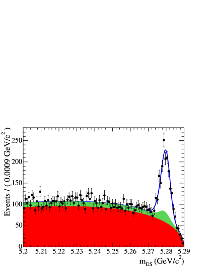
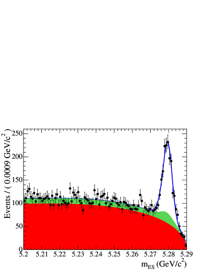
Figure 1: The $m_{\rm ES}$ distribution, together with the fitted PDFs: the data are the black points with statistical error bars, the lower solid (red/dark) area is the $q\overline{q}$ component, the middle solid (green/light) area is the $B\kern 1.79993pt\overline{\kern-1.79993ptB}{}$ background contribution, while the upper blue line shows the total fit result. The upper (lower) plot is for negatively charged (positively charged) events.

We independently fit the Dalitz plot of the negatively charged and positively charged samples to extract the magnitude and phase of the intermediate resonances and the nonresonant contribution using an unbinned maximum-likelihood fit. We construct a likelihood function:

$${\cal{L}}(x,y)=(1-f_{q\bar{q}}-f_{B\bar{B}})$$ (13)

$$\frac{\left|\sum_{j=1}^{N}c_{j}e^{i\theta_{j}}F_{j}(x,y)\right|^{2}\epsilon(x,y)}{\int~{}{|\sum_{j=1}^{N}c_{j}e^{i\theta_{j}}F_{j}(x,y)|^{2}\epsilon(x,y)}~{}dxdy}$$

$$+~{}f_{q\bar{q}}~{}\frac{Q(x,y)}{\int~{}Q(x,y)~{}dxdy}+~{}f_{B\bar{B}}~{}\frac{B(x,y)}{\int~{}B(x,y)~{}dxdy},$$

where $N$ is the number of resonant and nonresonant components in the model; $\epsilon(x,y)$ is the signal reconstruction efficiency defined for all points in the Dalitz plot; $Q(x,y)$ is the distribution of $q\overline{q}$ continuum background; $B(x,y)$ is the distribution of $B\kern 1.79993pt\overline{\kern-1.79993ptB}{}$ background; and $f_{q\overline{q}}$ and $f_{B\kern 1.25995pt\overline{\kern-1.25995ptB}{}}$ are the fractions of $q\overline{q}$ continuum and $B\kern 1.79993pt\overline{\kern-1.79993ptB}{}$ background components determined as described above and fixed in the Dalitz-plot fit.

To allow comparison among experiments we present fit fractions (FF) rather than amplitude magnitudes where the fit fraction is defined as the integral of a single decay amplitude squared divided by the coherent matrix element squared for the complete Dalitz plot:

$${\it FF}_{j}=\frac{\int\left|c_{j}e^{i\theta_{j}}F_{j}(x,y)\right|^{2}dxdy}{\int\left|\sum_{j}c_{j}e^{i\theta_{j}}F_{j}(x,y)\right|^{2}dxdy}.$$ (14)

The sum of all the fit fractions is not necessarily unity due to the potential presence of net constructive or destructive interference. The fit fraction asymmetry is defined as the difference over the sum of the $B^{-}\rightarrow\mbox{$K^{-}\pi^{+}\pi^{-}$}$ and $B^{+}\rightarrow\mbox{$K^{+}\pi^{-}\pi^{+}$}$ fit fractions:

$$A_{C\!P}^{j}=\frac{\overline{\it FF}_{j}-{\it FF}_{j}}{\overline{\it FF}_{j}+{\it FF}_{j}}.$$ (15)

The $q\overline{q}$ continuum and $B\kern 1.79993pt\overline{\kern-1.79993ptB}{}$ backgrounds are modeled as two-dimensional histograms ($m_{K^{+}\pi^{-}}^{2}$ vs. $m_{\pi^{+}\pi^{-}}^{2}$) for the $B^{+}$ and $B^{-}$ samples with bins of size $0.4({\mathrm{\,Ge\kern-1.00006ptV\!/}c^{2}})^{2}\times 0.4({\mathrm{\,Ge\kern-1.00006ptV\!/}c^{2}})^{2}$ with linear interpolation applied between bins. The $B\kern 1.79993pt\overline{\kern-1.79993ptB}{}$ background distributions are taken from MC studies and the $q\overline{q}$  distribution is taken from the $m_{\rm ES}$ sideband data. We expect from MC studies $1515\pm 59$ $B\kern 1.79993pt\overline{\kern-1.79993ptB}{}$ background events in the sideband region ($776\pm 37$ for negative events and $739\pm 36$ for positive events), which is 10.8% of the reconstructed sideband events. The distribution of these events is subtracted from the $q\overline{q}$ distribution. In order to increase the statistical precision of this distribution we then add off-resonance data events. This increases the sample size by 1202 events (605 for negative events and 597 for positive events). The Dalitz plot of the data in the signal region after subtraction of the two background distributions can be seen in Fig. 2.

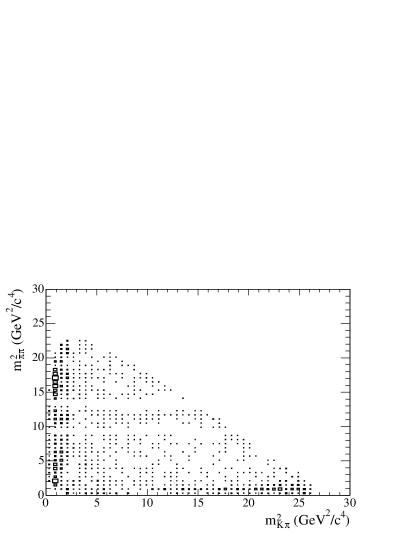
Figure 2: Background subtracted Dalitz plot of the combined $B^{\pm}\rightarrow\mbox{$K^{\pm}\pi^{\mp}\pi^{\pm}$}$ data sample in the signal region. The plot shows bins with greater than zero entries, the area of the boxes being proportional to the number of entries.

The two-dimensional efficiency distribution over the Dalitz plot $\epsilon(x,y)$ is calculated with 1.3 million $B^{\pm}\rightarrow\mbox{$K^{\pm}\pi^{\mp}\pi^{\pm}$}$ nonresonant MC events. All selection criteria are applied except for those corresponding to the invariant mass veto regions. The quotient is taken of two histograms, the denominator containing the true Dalitz-plot distribution of the MC events and the numerator containing the reconstructed MC events with corrections applied for differences between MC and data in the particle identification and tracking efficiencies. The efficiency shows very little variation across the majority of the Dalitz plot but there are decreases towards the corners where one of the particles has a low momentum. No difference in efficiency is seen between $B^{+}$ and $B^{-}$. The effect of experimental resolution on the signal model is neglected since the resonances under consideration are sufficiently broad. The average reconstruction efficiency for events in the signal box for the nonresonant MC sample is 16.7%.

For most resonant amplitudes the pole masses and widths are taken from the standard Particle Data Group tables Eidelman et al. (2004). However, there are no consistent measurements for the coupling constants $g_{\pi}$, $g_{K}$ and the pole mass $m_{0}$ of the $f_{0}(980)$ Ablikim et al. (2004); Aitala et al. (2001); Armstrong et al. (1991). We employ a likelihood scanning technique in order to determine the best-fit values: $g_{\pi}=0.11$, $g_{K}=0.36$ and $m_{0}=0.965{\mathrm{\,Ge\kern-1.00006ptV\!/}c^{2}}$. The $0^{+}$ component of the $K^{+}\pi^{-}$ spectrum, which we denote $(K\pi)^{*0}_{0}$, is poorly understood Aston et al. (1988); Dunwoodie ; Bugg (2003); we use the LASS parameterization Aston et al. (1988); Dunwoodie which consists of the $K^{*0}_{0}(1430)$ resonance together with an effective range nonresonant component.

$${\cal M} = \frac{m_{K\pi}}{q\cot{\delta_{B}}-iq}$$

$$+ e^{2i\delta_{B}}\frac{m_{0}\Gamma_{0}\frac{m_{0}}{q_{0}}}{(m_{0}^{2}-m_{K\pi}^{2})-im_{0}\Gamma_{0}\frac{q}{m_{K\pi}}\frac{m_{0}}{q_{0}}},$$

where $\cot{\delta_{B}}=\frac{1}{aq}+\mbox{${1\over 2}$}rq$. We have used the following values for the scattering length and effective range parameters of this distribution: $a=2.07\pm 0.10\,(\!{\mathrm{\,Ge\kern-1.00006ptV\!/}c})^{-1}$ and $r=3.32\pm 0.34\,(\!{\mathrm{\,Ge\kern-1.00006ptV\!/}c})^{-1}$ Dunwoodie . It has been shown in the decay $B\rightarrow{J\mskip-3.0mu/\mskip-2.0mu\psi\mskip 2.0mu}K\pi$ that the $P-S$ phase behaviour well matches that observed in the LASS experiment Aubert et al. (2005). But since this parameterization is only tested up to around 1.6${\mathrm{\,Ge\kern-1.00006ptV\!/}c^{2}}$ we curtail the effective range term at the $\kern 1.99997pt\overline{\kern-1.99997ptD}{}^{0}$ veto. Integrating separately the resonant part, the effective range part and the coherent sum we find that the $K^{*0}_{0}(1430)$ resonance accounts for 81%, the effective range term 45%, and the destructive interference between the two terms the excess 26% of $(K\pi)^{*0}_{0}$.

The nominal model comprises a phase-space nonresonant component and five intermediate resonance states: $\mbox{$K^{*0}(892)$}\pi^{+}$, $\mbox{$(K\pi)^{*0}_{0}$}\pi^{+}$, $\mbox{$\mbox{$\rho^{0}$}(770)$}K^{+}$, $\mbox{$f_{0}(980)$}K^{+}$, $\chi_{c0}K^{+}$. We choose this model using information from previous studies Aubert et al. (2004b) and the change in the goodness-of-fit observed when omitting or adding resonances. The nonresonant component is modeled with a constant complex amplitude. Alternative models for the nonresonant components, such as that proposed in Garmash et al. (2005), were also tested and found to make negligible difference to the measured parameters. The results of the fit with the nominal six-component model are shown in Table 1 separately for $B^{-}$ and $B^{+}$ data. The statistical errors are calculated from MC experiments where the events are generated from the PDFs used in the fit to data. The $\mbox{$\rho^{0}$}(770)$ resonance shows the greatest difference in fit fractions between the two samples. The projection plots of the fit can be seen in Fig. 3. For the $m_{K^{\pm}\pi^{\mp}}$ plots the requirement is made that $m_{\pi^{\pm}\pi^{\mp}}$ is greater than $2{\mathrm{\,Ge\kern-1.00006ptV\!/}c^{2}}$ and vice versa in order to better illustrate the structures present. Using the fitted signal distribution we calculate the average reconstruction efficiency for our signal sample to be 14.7%. This value, which includes all corrections due to differences between data and MC, can be used to calculate the inclusive branching fraction from the signal yield results.

As a measure of goodness-of-fit we evaluate the $\chi^{2}$ across the Dalitz plot. A 75 by 75 bin histogram is used and a minimum of 10 entries per bin is required (for those cases where this requirement is not met then neighbouring bins are combined). The results for $B^{-}$ ($B^{+}$) are a $\chi^{2}$ of 123 (148) for a total number of 116 (121) bins and 10 free parameters in both cases. We also calculate the same $\chi^{2}$ neglecting the region $1.2<m_{\pi^{\pm}\pi^{\mp}}<1.6{\mathrm{\,Ge\kern-1.00006ptV\!/}c^{2}}$ where there is no resonant component in the nominal fit model. The results for $B^{-}$ ($B^{+}$) are a $\chi^{2}$ of 109 (112) for a total number of 108 (109) bins and again 10 free parameters in both cases.

The omission of any of the nominal components from the fit results in a significantly worse negative log-likelihood with the fitted fractions and phases of the remaining components varying outside their error bounds.

Table 1: Final results of fits, with statistical, systematic and model-dependence errors, to $B^{-}$ and $B^{+}$ data with the six component model.

Component	$B^{-}$ Fit	$B^{+}$ Fit
$K^{*0}(892)$ Fraction (%)	$15.0\pm 1.6\pm 0.6^{+0.5}_{-1.3}$	$13.1\pm 1.5\pm 0.6^{+0.7}_{-1.2}$
$K^{*0}(892)$ Magnitude	$1.0$ FIXED	$1.0$ FIXED
$K^{*0}(892)$ Phase	$0.0$ FIXED	$0.0$ FIXED
$(K\pi)^{*0}_{0}$ Fraction(%)	$49.6\pm 2.4\pm 0.7^{+0.8}_{-5.0}$	$56.4\pm 2.4\pm 0.7^{+3.3}_{-5.2}$
$(K\pi)^{*0}_{0}$ Magnitude	$1.82\pm 0.12\pm 0.04^{+0.07}_{-0.09}$	$2.08\pm 0.15\pm 0.06^{+0.11}_{-0.14}$
$(K\pi)^{*0}_{0}$ Phase	$-0.38\pm 0.12\pm 0.03^{+0.08}_{-0.05}$	$0.01\pm 0.12\pm 0.03\pm 0.06$
$\mbox{$\rho^{0}$}(770)$ Fraction (%)	$10.5\pm 1.7\pm 0.4^{+0.6}_{-2.5}$	$5.4\pm 1.3\pm 0.5^{+0.9}_{-1.4}$
$\mbox{$\rho^{0}$}(770)$ Magnitude	$0.837\pm 0.079\pm 0.031^{+0.016}_{-0.076}$	$0.642\pm 0.092\pm 0.042^{+0.060}_{-0.076}$
$\mbox{$\rho^{0}$}(770)$ Phase	$-0.55\pm 0.38\pm 0.08^{+0.75}_{-0.65}$	$1.19\pm 0.62\pm 0.16^{+0.95}_{-0.57}$
$f_{0}(980)$ Fraction (%)	$16.1\pm 2.1\pm 0.4^{+1.1}_{-2.1}$	$13.5\pm 1.9\pm 0.4^{+0.7}_{-2.5}$
$f_{0}(980)$ Magnitude	$1.037\pm 0.080\pm 0.026^{+0.053}_{-0.072}$	$1.015\pm 0.095\pm 0.036^{+0.059}_{-0.092}$
$f_{0}(980)$ Phase	$1.23\pm 0.34\pm 0.07^{+0.69}_{-0.52}$	$2.29\pm 0.56\pm 0.13^{+1.39}_{-0.56}$
$\chi_{c0}$ Fraction (%)	$0.84\pm 0.44\pm 0.14^{+0.07}_{-0.08}$	$1.20\pm 0.50\pm 0.13^{+0.07}_{-0.08}$
$\chi_{c0}$ Magnitude	$0.237\pm 0.047\pm 0.009^{+0.018}_{-0.013}$	$0.302\pm 0.052\pm 0.016^{+0.016}_{-0.016}$
$\chi_{c0}$ Phase	$2.55\pm 0.40\pm 0.09^{+0.35}_{-0.11}$	$-2.52\pm 0.37\pm 0.35^{+0.18}_{-0.17}$
Nonresonant Fraction (%)	$4.3\pm 1.3\pm 0.8^{+1.3}_{-1.4}$	$4.6\pm 1.5\pm 0.9^{+1.8}_{-0.4}$
Nonresonant Magnitude	$0.54\pm 0.07\pm 0.06^{+0.10}_{-0.10}$	$0.60\pm 0.11\pm 0.06^{+0.09}_{-0.01}$
Nonresonant Phase	$-2.29\pm 0.33\pm 0.09^{+0.61}_{-0.40}$	$-1.85\pm 0.28\pm 0.07^{+0.38}_{-0.26}$

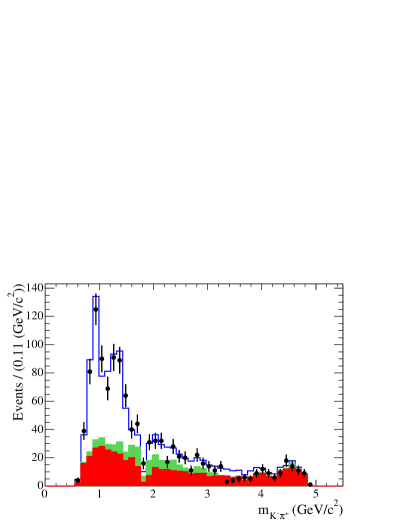
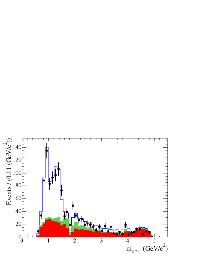
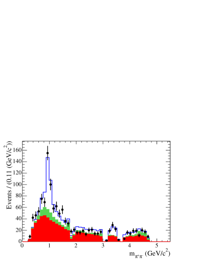
Figure 3: Invariant mass projections for the data in the signal region and the fit results. The upper (lower) plots are for the $B^{-}$ ($B^{+}$) sample. The left-hand (right-hand) plots show the $m_{K^{\pm}\pi^{\mp}}$ ($m_{\pi^{\pm}\pi^{\mp}}$) spectrum. The data are the black points with statistical error bars, the lower solid (red/dark) histogram is the $q\overline{q}$ component, the middle solid (green/light) histogram is the $B\kern 1.79993pt\overline{\kern-1.79993ptB}{}$ background contribution, while the upper blue histogram shows the total fit result. The large dips in the spectra correspond to the charm vetoes. For the $m_{K^{\pm}\pi^{\mp}}$ plots the requirement is made that $m_{\pi^{\pm}\pi^{\mp}}$ is greater than $2{\mathrm{\,Ge\kern-1.00006ptV\!/}c^{2}}$ and vice versa.

We have tested for the sensitivity of these results to additional resonances that can be added in the fit function. In the $\pi\pi$ spectrum there are possible higher resonances including $f_{2}(1270)$, $f_{0}(1370)$, $\mbox{$\rho^{0}$}(1450)$, $f_{0}(1500)$and $f^{\prime}_{2}(1525)$; in the $K\pi$ spectrum there are possible $K^{*0}_{2}(1430)$ and $K^{*0}(1680)$ resonances. Each of these resonances is added in turn to the nominal signal model, to form an extended model, and the Dalitz-plot fit is repeated. In general, adding another component does not significantly affect the measured fit fractions and phases of the six nominal components. We place upper limits on each of the possible additional components (Table 2).

The systematic uncertainties that affect the measurement of the fit fractions and phases are evaluated separately for $B^{-}$ and $B^{+}$. Each bin of the efficiency, $q\overline{q}$ and $B\kern 1.79993pt\overline{\kern-1.79993ptB}{}$ background histograms is fluctuated independently in accordance with its errors and the nominal fit repeated. The fractions of $B\kern 1.79993pt\overline{\kern-1.79993ptB}{}$ and $q\overline{q}$ events are varied in accordance with their errors and the fits repeated. To confirm the fitting procedure, 500 MC experiments were performed in which the events are generated from the PDFs used in the fit to data. A small fit bias is observed for the $\chi_{c0}$ and nonresonant components and is included in the systematic uncertainties. There is a contribution to the fit fraction asymmetry from possible detector charge bias, which has been estimated in previous studies to be 1% Aubert et al. (2003). A 0.4% systematic error on the total branching fraction comes from the error on the predicted number of $B\kern 1.79993pt\overline{\kern-1.79993ptB}{}$ background events. The systematic uncertainties for particle identification and tracking efficiency corrections are 4.2% and 2.4% respectively. The calculation of $N_{B\kern 1.25995pt\overline{\kern-1.25995ptB}{}}$ has a total uncertainty of 1.1%. The efficiency corrections due to the selection requirements on $\cos{\theta_{T}}$, the Fisher discriminant, $\Delta E$ and $m_{\rm ES}$ have also been calculated from $B^{+}\rightarrow\mbox{$\kern 1.99997pt\overline{\kern-1.99997ptD}{}^{0}\pi^{+}$}$, $\kern 1.99997pt\overline{\kern-1.99997ptD}{}^{0}\rightarrow K^{+}\pi^{-}$ data and MC samples, and the error on these corrections is incorporated into the branching fraction systematic uncertainties.

In addition to the above systematic uncertainties we also calculate a model-dependence uncertainty that characterizes the uncertainty on the results due to elements of the signal Dalitz-plot model. The first of these elements consists of the two parameters of the LASS model of the $K\pi$ S-wave and is calculated by refitting adjusting the parameters of the LASS model within their experimental errors. The second consists of the three parameters of the $f_{0}(980)$ resonance and is evaluated by refitting with the parameter values measured by the BES collaboration Ablikim et al. (2004). The third element is due to the different possible models for the nonresonant component and is evaluated by refitting with the parameterization proposed by Belle Garmash et al. (2005). The fourth element is the uncertainty due to the composition of the signal model and reflects observed changes in the parameters of the nominal components when the data are fitted with the extended models. The uncertainties from each of these elements are added in quadrature to give the final model-dependence uncertainty.

Table 2: Summary of measurements of branching fractions (averaged over charge conjugate states) and $C\!P$ asymmetries. The first error is statistical, the second is systematic and the third represents the model dependence.

Mode	${\cal B}(B^{+}\rightarrow{\rm Mode})(10^{-6})$	90% CL UL $(10^{-6})$	$A_{C\!P}$ (%)
$K^{+}\pi^{-}\pi^{+}$ Total	$64.1\pm 2.4\pm 4.0$	$-$	$-1.3\pm 3.7\pm 1.1$
$\mbox{$K^{*0}(892)$}\pi^{+}$; $\mbox{$K^{*0}(892)$}\rightarrow K^{+}\pi^{-}$	$8.99\pm 0.78\pm 0.48^{+0.28}_{-0.39}$	$-$	$6.8\pm 7.8\pm 5.7^{+4.0}_{-3.5}$
$\mbox{$(K\pi)^{*0}_{0}$}\pi^{+}$; $\mbox{$(K\pi)^{*0}_{0}$}\rightarrow K^{+}\pi^{-}$	$34.0\pm 1.7\pm 1.5^{+1.2}_{-1.6}$	$-$	$-6.4\pm 3.2\pm 2.0^{+1.1}_{-1.7}$
$\mbox{$\mbox{$\rho^{0}$}(770)$}K^{+}$; $\mbox{$\mbox{$\rho^{0}$}(770)$}\rightarrow\pi^{+}\pi^{-}$	$5.07\pm 0.75\pm 0.35^{+0.42}_{-0.68}$	$-$	$32\pm 13\pm 6^{+8}_{-5}$
$\mbox{$f_{0}(980)$}K^{+}$; $\mbox{$f_{0}(980)$}\rightarrow\pi^{+}\pi^{-}$	$9.47\pm 0.97\pm 0.46^{+0.42}_{-0.75}$	$-$	$8.8\pm 9.5\pm 2.6^{+9.3}_{-5.0}$
$\chi_{c0}K^{+}$; $\chi_{c0}\rightarrow\pi^{+}\pi^{-}$	$0.66\pm 0.22\pm 0.07\pm 0.03$	$<1.1$	$-$
$K^{+}\pi^{-}\pi^{+}$ nonresonant	$2.85\pm 0.64\pm 0.41^{+0.70}_{-0.34}$	$<6.5$	$-$
$\mbox{$K^{*0}_{2}(1430)$}\pi^{+}$; $\mbox{$K^{*0}_{2}(1430)$}\rightarrow K^{+}\pi^{-}$	$-$	$<7.7$	$-$
$\mbox{$K^{*0}(1680)$}\pi^{+}$; $\mbox{$K^{*0}(1680)$}\rightarrow K^{+}\pi^{-}$	$-$	$<3.8$	$-$
$\mbox{$f_{2}(1270)$}K^{+}$; $\mbox{$f_{2}(1270)$}\rightarrow\pi^{+}\pi^{-}$	$-$	$<8.9$	$-$
$\mbox{$f_{0}(1370)$}K^{+}$; $\mbox{$f_{0}(1370)$}\rightarrow\pi^{+}\pi^{-}$	$-$	$<10.7$	$-$
$\mbox{$\mbox{$\rho^{0}$}(1450)$}K^{+}$; $\mbox{$\mbox{$\rho^{0}$}(1450)$}\rightarrow\pi^{+}\pi^{-}$	$-$	$<11.7$	$-$
$\mbox{$f_{0}(1500)$}K^{+}$; $\mbox{$f_{0}(1500)$}\rightarrow\pi^{+}\pi^{-}$	$-$	$<4.4$	$-$
$\mbox{$f^{\prime}_{2}(1525)$}K^{+}$; $\mbox{$f^{\prime}_{2}(1525)$}\rightarrow\pi^{+}\pi^{-}$	$-$	$<3.4$	$-$

In order to make comparisons with previous measurements and predictions from factorization models we multiply each fit fraction by the total branching fraction to calculate the branching fraction of the mode. These branching fractions from each of the charge-separated fits are then averaged. For components that do not have statistically significant branching fractions 90% confidence level upper limits are determined. Upper limits are also calculated for the components added in the extended signal models. Upper limits are calculated from MC experiments where each experiment is generated from the fitted PDFs but with all sources of systematic uncertainty varied in accordance with their errors. The measured branching fractions, averaged over charge-conjugate states, and $C\!P$ asymmetries from this analysis are summarized in Table 2. Charge conjugates are included implicitly throughout this table and the following discussion.

The total $B^{\pm}\rightarrow\mbox{$K^{\pm}\pi^{\mp}\pi^{\pm}$}$ branching fraction ($(64.1\pm 2.4\pm 4.0)\times 10^{-6}$) has been measured with increased statistical accuracy and is compatible with previous BABAR measurements. It differs from Belle’s measurement of $(46.6\pm 2.1\pm 4.3)\times 10^{-6}$ Garmash et al. (2005), which is significantly smaller, even after accounting for the $\chi_{c0}K^{+}$ mode, which Belle does not include. This result was cross checked by using the same procedure to measure the $B^{+}\rightarrow\mbox{$\kern 1.99997pt\overline{\kern-1.99997ptD}{}^{0}\pi^{+}$}$; $\kern 1.99997pt\overline{\kern-1.99997ptD}{}^{0}\rightarrow K^{+}\pi^{-}$ branching fraction, which was found to be consistent with the PDG value Eidelman et al. (2004). The total charge asymmetry has been measured to be consistent with zero to a higher degree of precision than previous measurements.

After correcting for the secondary branching fraction ${\cal B}(\mbox{$\mbox{$K^{*0}(892)$}\rightarrow K^{+}\pi^{-}$})={2\over 3}$ we find the $B^{+}\rightarrow\mbox{$\mbox{$K^{*0}(892)$}\pi^{+}$}$ branching fraction to be: $(13.5\pm 1.2\pm 0.7^{+0.4}_{-0.6})\times 10^{-6}$. This is smaller than that measured in previous analyses that do not perform an amplitude fit to the Dalitz plot Aubert et al. (2004b); Abe et al. (2002) but slightly larger than the value reported by Belle in their amplitude analysis Garmash et al. (2005). The branching fraction measurement of $B^{+}\rightarrow\mbox{$\mbox{$\mbox{$\rho^{0}$}(770)$}K^{+}$}$ is the first measurement of the mode from BABAR and is consistent with that from Belle Garmash et al. (2005). It is also broadly compatible with many theoretical predictions Aleksan et al. (2003); de Groot et al. (2003); Du et al. (2002); Beneke and Neubert (2003); Chiang et al. (2004). The $B^{+}\rightarrow\mbox{$\mbox{$f_{0}(980)$}K^{+}$}$ branching fraction is in good agreement with earlier analyses Aubert et al. (2004b); Abe et al. (2002) and the recent Belle amplitude analysis Garmash et al. (2005). The forward-backward asymmetry apparent in both the $K^{*0}(892)$ and $f_{0}(980)$ bands in Fig. 2 is well reproduced by the fit and is not due to reconstruction efficiency effects but to $S-P$ interference in the Dalitz plot.

The $(K\pi)^{*0}_{0}$ component appears to be well modeled by the LASS parameterization, which consists of a nonresonant effective range term plus a relativistic Breit–Wigner term for the $K^{*0}_{0}(1430)$ resonance itself. Removing the phase-space nonresonant component from the nominal model gives very little change in the goodness-of-fit $\chi^{2}$ or the fit likelihood. It is unclear whether this component is required in addition to the nonresonant part of the $(K\pi)^{*0}_{0}$ component. We can calculate the branching fraction for $B^{+}\rightarrow\mbox{$\mbox{$K^{*0}_{0}(1430)$}\pi^{+}$}$ using our knowledge of the composition of the $(K\pi)^{*0}_{0}$ component and find it to be: $(44.4\pm 2.2\pm 2.0^{+1.6}_{-2.1}\pm 4.5)\times 10^{-6}$, where the fourth error is due to the uncertainty on the branching fraction of $\mbox{$K^{*0}_{0}(1430)$}\rightarrow K\pi$ combined with the uncertainty on the proportion of the $(K\pi)^{*0}_{0}$ component due to the $K^{*0}_{0}(1430)$ resonance. The Belle collaboration finds a similarly large $K^{*0}_{0}(1430)$ branching fraction though they treat the $K^{*0}_{0}(1430)$ as a separate component from the rest of the S-wave, modeled as a nonresonant component that has variation in magnitude but no variation in phase over the Dalitz plot Garmash et al. (2005).

For $B^{+}\rightarrow\mbox{$\mbox{$\mbox{$\rho^{0}$}(770)$}K^{+}$}$ and $B^{+}\rightarrow\mbox{$\chi_{c0}K^{+}$}$ the differences in phase between the $B^{+}$ and $B^{-}$ decays are $1.74\pm 0.73$ (2.4 standard deviations, $\sigma$) and $1.21\pm 0.54$ ($2.2\sigma$) respectively, where the errors are statistical only. The $\mbox{$K^{*0}(892)$}\pi^{+}$ charge asymmetry is consistent with zero, as expected from the Standard Model predictions Aleksan et al. (2003); de Groot et al. (2003); Du et al. (2002); Beneke and Neubert (2003); Chiang et al. (2004). There is no evidence of new physics entering the penguin diagram loop.

We are grateful for the excellent luminosity and machine conditions provided by our PEP-II colleagues, and for the substantial dedicated effort from the computing organizations that support BABAR. The collaborating institutions wish to thank SLAC for its support and kind hospitality. This work is supported by DOE and NSF (USA), NSERC (Canada), IHEP (China), CEA and CNRS-IN2P3 (France), BMBF and DFG (Germany), INFN (Italy), FOM (The Netherlands), NFR (Norway), MIST (Russia), and PPARC (United Kingdom). Individuals have received support from CONACyT (Mexico), A. P. Sloan Foundation, Research Corporation, and Alexander von Humboldt Foundation.

References

Kobayashi and Maskawa (1973)
M. Kobayashi and
T. Maskawa,
Prog. Theor. Phys. 49,
652 (1973).
Aleksan et al. (2003)
R. Aleksan,
P. F. Giraud,
V. Morenas,
O. Pene, and
A. S. Safir,
Phys. Rev. D67,
094019 (2003).
de Groot et al. (2003)
N. de Groot,
W. N. Cottingham,
and I. B.
Whittingham, Phys. Rev.
D68, 113005
(2003).
Du et al. (2002)
D.-s. Du,
H.-j. Gong,
J.-f. Sun,
D.-s. Yang, and
G.-h. Zhu,
Phys. Rev. D65,
094025 (2002).
Beneke and Neubert (2003)
M. Beneke and
M. Neubert,
Nucl. Phys. B675,
333 (2003).
Chiang et al. (2004)
C.-W. Chiang,
M. Gronau,
Z. Luo,
J. L. Rosner,
and D. A.
Suprun, Phys. Rev.
D69, 034001
(2004).
Aubert et al. (2002a)
B. Aubert et al.
(BABAR), Nucl. Instrum. Meth.
A479, 1
(2002a).
Kozanecki (2000)
W. Kozanecki,
Nucl. Instrum. Meth. A446,
59 (2000).
Fleming (1964)
G. N. Fleming,
Phys. Rev. 135,
B551 (1964).
Morgan (1968)
D. Morgan,
Phys. Rev. 166,
1731 (1968).
Herndon et al. (1975)
D. Herndon,
P. Soding, and
R. J. Cashmore,
Phys. Rev. D11,
3165 (1975).
Blatt and Weisskopf (1952)
J. Blatt and
V. E. Weisskopf,
Theoretical Neuclear Physics (J.
Wiley (New York), 1952).
Eidelman et al. (2004)
S. Eidelman et al.
(Particle Data Group), Phys.
Lett. B592, 1
(2004).
(14)
D. V. Bugg,
private communication.
Flatte (1976)
S. M. Flatte,
Phys. Lett. B63,
224 (1976).
Zemach (1964)
C. Zemach,
Phys. Rev. 133,
B1201 (1964).
Zemach (1965)
C. Zemach,
Phys. Rev. 140,
B97 (1965).
Asner (2003)
D. Asner (2003),
eprint hep-ex/0410014.
Fisher (1936)
R. A. Fisher,
Annals Eugen. 7,
179 (1936).
Aubert et al. (2002b)
B. Aubert et al.
(BABAR), Phys. Rev. Lett.
89, 281802
(2002b).
Aubert et al. (2004a)
B. Aubert et al.
(BABAR), Phys. Rev. Lett.
93, 231801
(2004a).