Determination of the $b$-quark leading shape function parameters in the shape function scheme using the Belle $B\to X_{s}\gamma$ photon energy spectrum

Abstract

We determine the $b$-quark shape function parameters in the shape function scheme, $m_{b}(\rm SF)$ and $\mu_{\pi}^{2}(\rm SF)$  using the Belle $B\to X_{s}\gamma$ photon energy spectrum. We assume three models for the form of the shape function; exponential, gaussian and hyperbolic.

I Introduction

One of the best ways to determine the Cabbibo-Kobayashi-Maskawa(CKM) matrix element $|V_{ub}|$ is to measure the inclusive charmless semileptonic ($B\to X_{u}\ell\nu$) partial branching fraction of the $B$ meson. Its theoretical prediction relies on an accurate description of non-perturbative bound-state effects of a $b$ quark in the $B$ meson. The effects are encoded in $B$-meson shape functions, which are not theoretically calculable and have to be determined experimentally. The leading order shape function can be determined using the photon energy spectrum in $B\to X_{s}\gamma$ decays, since up to the leading order of $1/m_{b}$ in the Heavy Quark Expansion it is described with the same leading order shape function as the one used for the prediction of the $B\to X_{u}\ell\nu$ decays. Such shape function determination was first performed by CLEO on their $B\to X_{s}\gamma$ data Gibbons , and was then repeated in Ref. limonoz for the Belle $B\to X_{s}\gamma$ data, where the theory proposed by Kagan and Neubert KN was used to describe the photon energy spectrum.

Recently, Bosch, Lange, Neubert and Paz presented theoretical expressions for the triple differential $B\to X_{u}\ell\nu$ decay rates and for the $B\to X_{s}\gamma$ photon spectrum, which incorporate all known contributions and smoothly interpolate between the ”shape-function region” of large hadronic energy and small invariant mass, and the ”OPE region” (in which all hadronic kinematical variables scale with $M_{B}$) BLNP ; generator . The differential rate is given in terms of a leading shape function and a subleading shape function in the shape function scheme BLNP ; generator , where in this scheme the leading shape function is expressed with the parameters $m_{b}(\rm SF)$ and $\mu_{\pi}^{2}(\rm SF)$.

In this paper we report on the determination of the shape function parameters by fitting the Belle $B\to X_{s}\gamma$ data with the predicted photon energy spectrum generator , where the default subleading shape function model from Ref. generator is used. It allows for a precise determination of $|V_{ub}|$ as shown in Ref. endpoint and Ref. fullrec .

Apart from using an updated and more complete theoretical description of the $B\to X_{s}\gamma$ decays, this analysis differs from the one in Ref. limonoz by using a different set of shape function model parametrizations, namely exponential, gaussian and hyperbolic. It also includes subleading shape function effects that were absent in the former analysis.

II Procedure

We used a method based on that devised by the CLEO Collaboration Anderson . We fit Monte Carlo (MC) simulated spectra to the raw data photon energy spectrum. “Raw” refers to the spectra that are obtained after the application of the $B\to X_{s}\gamma$ analysis cuts. The use of “raw” spectra correctly accounts for Lorentz boost from the $B$ rest frame to the center of mass system, energy resolution effects and avoids unfolding. The method is as follows:

1. Assume a shape function model.

2. Simulate the photon energy spectrum for a certain set of parameters; ($m_{b}(\rm SF)$, $\mu_{\pi}^{2}(\rm SF)$).

3. Perform a $\chi^{2}$ fit of the simulated spectrum to the data where only the normalization of the simulated spectrum is floated and keep the resultant $\chi^{2}$ value.

4. Repeat steps 2-3 for different sets of parameters to construct a two dimensional grid with each point having a $\chi^{2}$.

5. Find the minimum $\chi^{2}$ on the grid and all points on the grid that are one unit of $\chi^{2}$ above the minimum.

6. Repeat steps 1-5 for a different shape function model.

II.1 Shape function models

Three shape function forms suggested in the literature are employed; exponential, gaussian and hyperbolic generator . Their functional forms are described in Table 1: they are a function of $\hat{\omega}$ and are parameterized by two parameters: $\Lambda$ and $b$. Example shape function forms are plotted in Fig. 1.

Shape Function	Form
exponential	$F^{\rm(exp)}(\hat{\omega};\Lambda,b)=\frac{N^{\rm(exp)}}{\Lambda}\left(\frac{\hat{\omega}}{\Lambda}\right)^{b-1}\exp\left(-d_{\rm exp}\frac{\hat{\omega}}{\Lambda}\right)$
gaussian	$F^{\rm(gauss)}(\hat{\omega};\Lambda,b)=\frac{N^{\rm(gauss)}}{\Lambda}\left(\frac{\hat{\omega}}{\Lambda}\right)^{b-1}\exp\left(-d_{\rm gauss}\frac{\hat{\omega}^{2}}{\Lambda^{2}}\right)$
hyperbolic	$F^{\rm(hyp)}(\hat{\omega};\Lambda,b)=\frac{N^{\rm(hyp)}}{\Lambda}\left(\frac{\hat{\omega}}{\Lambda}\right)^{b-1}\cosh^{-1}\left(d_{\rm hyp}\frac{\hat{\omega}}{\Lambda}\right)$
where the constants are:
$\begin{aligned} N^{\rm(exp)}&=\frac{d_{\rm(exp)}^{b}}{\Gamma(b)}\,,&d_{\rm(exp)}&=b\,,\\ N^{\rm(gauss)}&=\frac{2\,d_{\rm(gauss)}^{b/2}}{\Gamma(b/2)}\,,&d_{\rm(gauss)}&=\left(\frac{\Gamma\left(\frac{1+b}{2}\right)}{\Gamma\left(\frac{b}{2}\right)}\right)^{2}\,,\\ N^{\rm(hyp)}&=\frac{[4\,d_{\rm(hyp)}]^{b}}{2\,\Gamma(b)\left[\zeta(b,\frac{1}{4})-\zeta(b,\frac{3}{4})\right]}\,,&d_{\rm(hyp)}&=\frac{b}{4}\,\frac{\zeta\left(1+b,\frac{1}{4}\right)-\zeta\left(1+b,\frac{3}{4}\right)}{\zeta\left(b,\frac{1}{4}\right)-\zeta\left(b,\frac{3}{4}\right)}\,,\end{aligned}$
$\zeta(b,a)=\sum_{k=0}^{\infty}(k+a)^{-b}$ is the generalized Riemann zeta function

Table 1: The three models used for the shape function forms

The parameters $\Lambda$ and $b$ are related to the HQET parameters $\bar{\Lambda}$ and $\mu_{\pi}^{2}$ by analytical expressions Eq.46 and Eq.47 in Ref. generator for exponential and gaussian models, respectively, while for the hyperbolic model the corresponding HQET parameters have to be calculated numerically. The shape function parameters $m_{b}(\rm SF)$ and $\mu_{\pi}^{2}(\rm SF)$ are obtained from the HQET parameters $\bar{\Lambda}$ and $\mu_{\pi}^{2}$ using the relations in Eq.41 of Ref. generator , where the reference scale of $1.5\,{\rm GeV}$ is used.

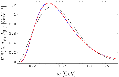
Figure 1: Three different models with linear onset for small $\hat{\omega}$. We show $F^{\rm(exp)}$ (solid), $F^{\rm(gauss)}$ (dashed), and $F^{\rm(hyp)}$ (dash-dotted), for parameters that correspond to $m_{b}(\rm SF)$= 4.63$\,{\rm GeV}/\mathit{c}^{2}$ and $\mu_{\pi}^{2}(\rm SF)$= 0.2 $\,{\rm GeV}^{2}/\mathit{c}^{2}$ generator .

II.2 Monte Carlo simulated photon energy spectrum

We generate $B\to X_{s}\gamma$ MC events according to the prescription in Ref. generator for each set of the shape function parameter values. The generated events are simulated for the detector performance using the Belle detector simulation program and the $B\to X_{s}\gamma$ analysis cuts are applied to the MC events to obtain the raw photon energy spectrum in the $\Upsilon(4S)$ rest frame Koppenburg .

II.3 Fitting the spectrum

For a given set of shape function parameters, a $\chi^{2}$ fit of the MC simulated photon spectrum to the raw data spectrum is performed in the interval $1.8<E^{*}_{\gamma}<2.8\,{\rm GeV}$ . Although in the Ref. limonoz the fitting was performed in the interval between $1.5\,{\rm GeV}$ and $2.8\,{\rm GeV}$, the data below $1.8\,{\rm GeV}$ are not used in the present analysis since the tails of the models we use below $1.8\,{\rm GeV}$ are not modelled accurately lange .

The normalization parameter is floated in the fit. The raw spectrum is plotted in Figure 2, the errors include both statistical and systematic errors. The latter are dominated by the estimation of the $B\overline{B}$ background and are 100% correlated. Therefore the covariance matrix is constructed as

$$V_{ij}=\sigma^{\mathrm{stat}}_{d_{i}}\sigma^{\mathrm{stat}}_{d_{j}}\delta_{ij}+\sigma^{\mathrm{sys}}_{d_{i}}\sigma^{\mathrm{sys}}_{d_{j}}$$ (1)

where $i,j=1,2,\ldots,10$ denote the bin number, and $\sigma_{d}$ is the error in the data. Then the $\chi^{2}$ used in the fitting is given by

$$\chi^{2}=\sum_{ij}(d_{i}-f_{i})(V^{-1})_{ij}(d_{j}-f_{j}),$$ (2)

where $(V^{-1})_{ij}$ denotes the $ij^{th}$ element of the inverted covariance matrix. The $\chi^{2}$ value of the fit is used to determine a map of $\chi^{2}$ as a function of the shape function parameters.

Figure 2: Raw $B\rightarrow X_{s}\gamma$ photon energy spectra in the $\Upsilon(4S)$ frame as acquired from data. The errors include both statistical and systematic errors. Raw refers to spectra as measured after the application of Belle $B\rightarrow X_{s}\gamma$ analysis cuts.

II.4 The best fit and $\Delta\chi^{2}$ contour

The best fit parameters are associated to the minimum chi-squared case, $\chi^{2}_{\mathrm{min}}$. The error “ellipse” is defined as the contour which satisfies $\Delta\chi^{2}\equiv\chi^{2}-\chi^{2}_{\mathrm{min}}=1$. The contours are found to be well approximated by the functionFac ,

$$\Delta\chi^{2}(m_{b}(\rm SF),\mu_{\pi}^{2}(\rm SF))=\left(\frac{\mu_{\pi}^{2}(\rm SF)+a(\mathit{m_{b}(\rm SF)})^{2}+b}{c}\right)^{2}+\left(\frac{(\mathit{m_{b}(\rm SF)})^{2}+d}{e}\right)^{2}.$$ (3)

The parameters $a$, $b$, $c$, $d$, and $e$ are determined by fitting the function to the parameter points that lie on the contour.

III Results

The best fit parameters are given in Table 2. The parameter values are found to be consistent across all three shape function forms. The minimum $\chi^{2}$ fit for each shape function model is displayed in Figure 3. The fits to the contour with $\Delta\chi^{2}=1$ points are shown in Figure 3 and 4. The imposed shape function form acts to correlate $m_{b}(\rm SF)$ and $\mu_{\pi}^{2}(\rm SF)$.

(a) exponential	(b) gaussian	(c) hyperbolic

Figure 3: Top: Minimum $\chi^{2}$ fits of MC simulated spectra to the raw data for each shape function model. Bottom: The fitted $\Delta\chi^{2}=1$ contours for each shape function model.

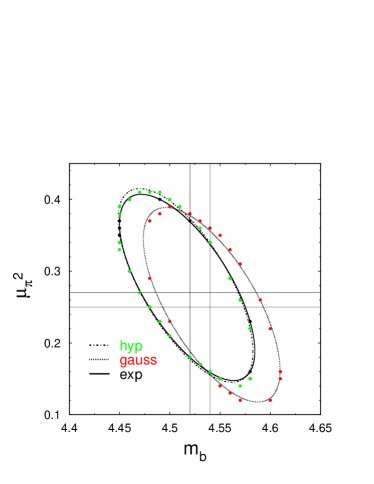
Figure 4: Comparison of the fitted $\Delta\chi^{2}=1$ contours for all shape function models. The contours for the exponential, gaussian and hyperbolic model are shown by the solid, dotted and dash-dotted curves, respectively. The vertical and horizontal lines mark the central values of the three fits.

Shape	$\chi^{2}_{\mathrm{min}}$	$m_{b}(\rm SF)$	$\mu_{\pi}^{2}(\rm SF)$
		$\mathrm{GeV}/c^{2}$	$\mathrm{GeV}^{2}/c^{2}$
exponential	4.32	4.52	0.27
gaussian	3.78	4.54	0.25
hyperbolic	4.41	4.52	0.27

Table 2: The best fit shape function parameter values.

IV Summary

The $b$-quark leading shape function parameters in the shape function scheme, $m_{b}(\rm SF)$ and $\mu_{\pi}^{2}(\rm SF)$, were determined from fits of Monte Carlo simulated spectra, generated by the prescription in Ref. generator , to the raw  Belle measured $B\to X_{s}\gamma$ photon energy spectrum. Three models for the form of the leading shape function were used; exponential, gaussian and hyperbolic, while the default model from Ref. generator was used for the subleading shape function, where the reference scale is chosen to be $1.5\,{\rm GeV}$. Best fit parameters are: $(m_{b}(\rm SF),\mu_{\pi}^{2}(\rm SF))_{\mathrm{exp}}=(4.52,0.27)$, $(m_{b}(\rm SF),\mu_{\pi}^{2}(\rm SF))_{\mathrm{gauss}}=(4.54,0.25)$, and $(m_{b}(\rm SF),\mu_{\pi}^{2}(\rm SF))_{\mathrm{hyp}}=(4.52,0.27)$, where $m_{b}(\rm SF)$ and $\mu_{\pi}^{2}(\rm SF)$ are measured in units of $\mathrm{GeV}/c^{2}$ and $\mathrm{GeV}^{2}/c^{2}$ respectively. We also determined the $\Delta\chi^{2}=1$ contours in the $(m_{b}(\rm SF),\mu_{\pi}^{2}(\rm SF))$ parameter space for each of the assumed models.

References

• (1) L.ย Gibbons [CLEO Collaboration], AIP Conf.ย Proc.ย  722, 156 (2004).
• (2) A.ย Limosani and T.ย Nozaki [Heavy Flavor Averaging Group], arXiv:hep-ex/0407052.
• (3) A.L. Kagan and M. Neubert, Eur. Phys. J. C7 5 (1999).
• (4) S.W. Bosch, B.O. Lange, M. Neubert and G. Paz, Nucl. Phys. Nucl.ย Phys.ย B 699, 335 (2004); M. Neubert, Eur. Phys. J. C (in print) [arXiv:hep-ph/0408179] ; S.W. Bosch, M. Neubert and G. Paz, JHEP 0411, 073 (2004); M. Neubert, arXiv:hep-ph/0411027; M. Neubert, arXiv:hep-ph/0412241.
• (5) B.O.ย Lange, M.ย Neubert and G.ย Paz, hep-ph/0504071 and private communication with M.ย Neubert.
• (6) A.ย Limosani et al. [Belle Collaboration], arXiv:hep-ex/0504046.
• (7) I.ย Bizjak et al. [Belle Collaboration], arXiv:hep-ex/0505088.
• (8) S. Anderson, Ph.D. thesis, University of Minnesota, 2002.
• (9) P.ย Koppenburg et al. [Belle Collaboration], Phys.ย Rev.ย Lett.ย  93, 061803 (2004).
• (10) We thank B. Lange for noticing us this fact.
• (11) We thank R. Faccini for suggesting such a function.