A Search for Supersymmetric Higgs Bosons in the Di-Tau Decay Mode in $p\bar{p}$ Collisions at $\sqrt{s}=1.8$ TeV

Abstract

A search for direct production of Higgs bosons in the di-tau decay mode is performed with $86.3\pm 3.5$ pb^-1 of data collected with the Collider Detector at Fermilab during the 1994$-$1995 data taking period of the Tevatron. We search for events where one tau decays to an electron plus neutrinos and the other tau decays hadronically. We perform a counting experiment and set limits on the cross section for supersymmetric Higgs boson production where $\tan{\beta}$ is large and $m_{A}$ is small. For a benchmark parameter space point where $m_{A^{0}}=100$ GeV/$c^{2}$ and $\tan{\beta}=50$, we limit the production cross section multiplied by the branching ratio to be less than 77.9 pb at the 95% confidence level compared to the theoretically predicted value of 11.0 pb. This is the first search for Higgs bosons decaying to tau pairs at a hadron collider.

D. Acosta,¹⁴ T. Affolder,⁷ M.G. Albrow,¹³ D. Ambrose,³⁶ D. Amidei,²⁷ K. Anikeev,²⁶ J. Antos,¹ G. Apollinari,¹³ T. Arisawa,⁵⁰ A. Artikov,¹¹ W. Ashmanskas,² F. Azfar,³⁴ P. Azzi-Bacchetta,³⁵ N. Bacchetta,³⁵ H. Bachacou,²⁴ W. Badgett,¹³ A. Barbaro-Galtieri,²⁴ V.E. Barnes,³⁹ B.A. Barnett,²¹ S. Baroiant,⁵ M. Barone,¹⁵ G. Bauer,²⁶ F. Bedeschi,³⁷ S. Behari,²¹ S. Belforte,⁴⁷ W.H. Bell,¹⁷ G. Bellettini,³⁷ J. Bellinger,⁵¹ D. Benjamin,¹² A. Beretvas,¹³ A. Bhatti,⁴¹ M. Binkley,¹³ D. Bisello,³⁵ M. Bishai,¹³ R.E. Blair,² C. Blocker,⁴ K. Bloom,²⁷ B. Blumenfeld,²¹ A. Bocci,⁴¹ A. Bodek,⁴⁰ G. Bolla,³⁹ A. Bolshov,²⁶ D. Bortoletto,³⁹ J. Boudreau,³⁸ C. Bromberg,²⁸ E. Brubaker,²⁴ J. Budagov,¹¹ H.S. Budd,⁴⁰ K. Burkett,¹³ G. Busetto,³⁵ K.L. Byrum,² S. Cabrera,¹² M. Campbell,²⁷ W. Carithers,²⁴ D. Carlsmith,⁵¹ A. Castro,³ D. Cauz,⁴⁷ A. Cerri,²⁴ L. Cerrito,²⁰ J. Chapman,²⁷ C. Chen,³⁶ Y.C. Chen,¹ M. Chertok,⁵ G. Chiarelli,³⁷ G. Chlachidze,¹³ F. Chlebana,¹³ M.L. Chu,¹ J.Y. Chung,³² W.-H. Chung,⁵¹ Y.S. Chung,⁴⁰ C.I. Ciobanu,²⁰ A.G. Clark,¹⁶ M. Coca,⁴⁰ A. Connolly,²⁴ M. Convery,⁴¹ J. Conway,⁴³ M. Cordelli,¹⁵ J. Cranshaw,⁴⁵ R. Culbertson,¹³ D. Dagenhart,⁴ S. D’Auria,¹⁷ P. de Barbaro,⁴⁰ S. De Cecco,⁴² S. Dell’Agnello,¹⁵ M. Dell’Orso,³⁷ S. Demers,⁴⁰ L. Demortier,⁴¹ M. Deninno,³ D. De Pedis,⁴² P.F. Derwent,¹³ C. Dionisi,⁴² J.R. Dittmann,¹³ A. Dominguez,²⁴ S. Donati,³⁷ M. D’Onofrio,¹⁶ T. Dorigo,³⁵ N. Eddy,²⁰ R. Erbacher,¹³ D. Errede,²⁰ S. Errede,²⁰ R. Eusebi,⁴⁰ S. Farrington,¹⁷ R.G. Feild,⁵² J.P. Fernandez,³⁹ C. Ferretti,²⁷ R.D. Field,¹⁴ I. Fiori,³⁷ B. Flaugher,¹³ L.R. Flores-Castillo,³⁸ G.W. Foster,¹³ M. Franklin,¹⁸ J. Friedman,²⁶ I. Furic,²⁶ M. Gallinaro,⁴¹ M. Garcia-Sciveres,²⁴ A.F. Garfinkel,³⁹ C. Gay,⁵² D.W. Gerdes,²⁷ E. Gerstein,⁹ S. Giagu,⁴² P. Giannetti,³⁷ K. Giolo,³⁹ M. Giordani,⁴⁷ P. Giromini,¹⁵ V. Glagolev,¹¹ D. Glenzinski,¹³ M. Gold,³⁰ N. Goldschmidt,²⁷ J. Goldstein,³⁴ G. Gomez,⁸ M. Goncharov,⁴⁴ I. Gorelov,³⁰ A.T. Goshaw,¹² Y. Gotra,³⁸ K. Goulianos,⁴¹ A. Gresele,³ C. Grosso-Pilcher,¹⁰ M. Guenther,³⁹ J. Guimaraes da Costa,¹⁸ C. Haber,²⁴ S.R. Hahn,¹³ E. Halkiadakis,⁴⁰ R. Handler,⁵¹ F. Happacher,¹⁵ K. Hara,⁴⁸ R.M. Harris,¹³ F. Hartmann,²² K. Hatakeyama,⁴¹ J. Hauser,⁶ J. Heinrich,³⁶ M. Hennecke,²² M. Herndon,²¹ C. Hill,⁷ A. Hocker,⁴⁰ K.D. Hoffman,¹⁰ S. Hou,¹ B.T. Huffman,³⁴ R. Hughes,³² J. Huston,²⁸ J. Incandela,⁷ G. Introzzi,³⁷ M. Iori,⁴² C. Issever,⁷ A. Ivanov,⁴⁰ Y. Iwata,¹⁹ B. Iyutin,²⁶ E. James,¹³ M. Jones,³⁹ T. Kamon,⁴⁴ J. Kang,²⁷ M. Karagoz Unel,³¹ S. Kartal,¹³ H. Kasha,⁵² Y. Kato,³³ R.D. Kennedy,¹³ R. Kephart,¹³ B. Kilminster,⁴⁰ D.H. Kim,²³ H.S. Kim,²⁰ M.J. Kim,⁹ S.B. Kim,²³ S.H. Kim,⁴⁸ T.H. Kim,²⁶ Y.K. Kim,¹⁰ M. Kirby,¹² L. Kirsch,⁴ S. Klimenko,¹⁴ P. Koehn,³² K. Kondo,⁵⁰ J. Konigsberg,¹⁴ A. Korn,²⁶ A. Korytov,¹⁴ J. Kroll,³⁶ M. Kruse,¹² V. Krutelyov,⁴⁴ S.E. Kuhlmann,² N. Kuznetsova,¹³ A.T. Laasanen,³⁹ S. Lami,⁴¹ S. Lammel,¹³ J. Lancaster,¹² M. Lancaster,²⁵ R. Lander,⁵ K. Lannon,³² A. Lath,⁴³ G. Latino,³⁰ T. LeCompte,² Y. Le,²¹ J. Lee,⁴⁰ S.W. Lee,⁴⁴ N. Leonardo,²⁶ S. Leone,³⁷ J.D. Lewis,¹³ K. Li,⁵² C.S. Lin,¹³ M. Lindgren,⁶ T.M. Liss,²⁰ D.O. Litvintsev,¹³ T. Liu,¹³ N.S. Lockyer,³⁶ A. Loginov,²⁹ M. Loreti,³⁵ D. Lucchesi,³⁵ P. Lukens,¹³ L. Lyons,³⁴ J. Lys,²⁴ R. Madrak,¹⁸ K. Maeshima,¹³ P. Maksimovic,²¹ L. Malferrari,³ M. Mangano,³⁷ G. Manca,³⁴ M. Mariotti,³⁵ M. Martin,²¹ A. Martin,⁵² V. Martin,³¹ M. Martínez,¹³ P. Mazzanti,³ K.S. McFarland,⁴⁰ P. McIntyre,⁴⁴ M. Menguzzato,³⁵ A. Menzione,³⁷ P. Merkel,¹³ C. Mesropian,⁴¹ A. Meyer,¹³ T. Miao,¹³ J.S. Miller,²⁷ R. Miller,²⁸ S. Miscetti,¹⁵ G. Mitselmakher,¹⁴ N. Moggi,³ R. Moore,¹³ T. Moulik,³⁹ A. Mukherjee,^M. Mulhearn,²⁶ T. Muller,²² A. Munar,³⁶ P. Murat,¹³ J. Nachtman,¹³ S. Nahn,⁵² I. Nakano,¹⁹ R. Napora,²¹ C. Nelson,¹³ T. Nelson,¹³ C. Neu,³² M.S. Neubauer,²⁶ C. Newman-Holmes,¹³ F. Niell,²⁷ T. Nigmanov,³⁸ L. Nodulman,² S.H. Oh,¹² Y.D. Oh,²³ T. Ohsugi,¹⁹ T. Okusawa,³³ W. Orejudos,²⁴ C. Pagliarone,³⁷ F. Palmonari,³⁷ R. Paoletti,³⁷ V. Papadimitriou,⁴⁵ J. Patrick,¹³ G. Pauletta,⁴⁷ M. Paulini,⁹ T. Pauly,³⁴ C. Paus,²⁶ D. Pellett,⁵ A. Penzo,⁴⁷ T.J. Phillips,¹² G. Piacentino,³⁷ J. Piedra,⁸ K.T. Pitts,²⁰ A. Pompoš,³⁹ L. Pondrom,⁵¹ G. Pope,³⁸ O. Poukov,¹¹ T. Pratt,³⁴ F. Prokoshin,¹¹ J. Proudfoot,² F. Ptohos,¹⁵ G. Punzi,³⁷ J. Rademacker,³⁴ A. Rakitine,²⁶ F. Ratnikov,⁴³ H. Ray,²⁷ A. Reichold,³⁴ P. Renton,³⁴ M. Rescigno,⁴² F. Rimondi,³ L. Ristori,³⁷ W.J. Robertson,¹² T. Rodrigo,⁸ S. Rolli,⁴⁹ L. Rosenson,²⁶ R. Roser,¹³ R. Rossin,³⁵ C. Rott,³⁹ A. Roy,³⁹ A. Ruiz,⁸ D. Ryan,⁴⁹ A. Safonov,⁵ R. St. Denis,¹⁷ W.K. Sakumoto,⁴⁰ D. Saltzberg,⁶ C. Sanchez,³² A. Sansoni,¹⁵ L. Santi,⁴⁷ S. Sarkar,⁴² P. Savard,⁴⁶ A. Savoy-Navarro,¹³ P. Schlabach,¹³ E.E. Schmidt,¹³ M.P. Schmidt,⁵² M. Schmitt,³¹ L. Scodellaro,³⁵ A. Scribano,³⁷ A. Sedov,³⁹ S. Seidel,³⁰ Y. Seiya,⁴⁸ A. Semenov,¹¹ F. Semeria,³ M.D. Shapiro,²⁴ P.F. Shepard,³⁸ T. Shibayama,⁴⁸ M. Shimojima,⁴⁸ M. Shochet,¹⁰ A. Sidoti,³⁵ A. Sill,⁴⁵ P. Sinervo,⁴⁶ A.J. Slaughter,⁵² K. Sliwa,⁴⁹ F.D. Snider,¹³ R. Snihur,²⁵ M. Spezziga,⁴⁵ L. Spiegel,¹³ F. Spinella,³⁷ M. Spiropulu,⁷ A. Stefanini,³⁷ J. Strologas,³⁰ D. Stuart,⁷ A. Sukhanov,¹⁴ K. Sumorok,²⁶ T. Suzuki,⁴⁸ R. Takashima,¹⁹ K. Takikawa,⁴⁸ M. Tanaka,² M. Tecchio,²⁷ P.K. Teng,¹ K. Terashi,⁴¹ R.J. Tesarek,¹³ S. Tether,²⁶ J. Thom,¹³ A.S. Thompson,¹⁷ E. Thomson,³² P. Tipton,⁴⁰ S. Tkaczyk,¹³ D. Toback,⁴⁴ K. Tollefson,²⁸ D. Tonelli,³⁷ M. Tönnesmann,²⁸ H. Toyoda,³³ W. Trischuk,⁴⁶ J. Tseng,²⁶ D. Tsybychev,¹⁴ N. Turini,³⁷ F. Ukegawa,⁴⁸ T. Unverhau,¹⁷ T. Vaiciulis,⁴⁰ A. Varganov,²⁷ E. Vataga,³⁷ S. Vejcik III,¹³ G. Velev,¹³ G. Veramendi,²⁴ R. Vidal,¹³ I. Vila,⁸ R. Vilar,⁸ I. Volobouev,²⁴ M. von der Mey,⁶ R.G. Wagner,² R.L. Wagner,¹³ W. Wagner,²² Z. Wan,⁴³ C. Wang,¹² M.J. Wang,¹ S.M. Wang,¹⁴ B. Ward,¹⁷ S. Waschke,¹⁷ D. Waters,²⁵ T. Watts,⁴³ M. Weber,²⁴ W.C. Wester III,¹³ B. Whitehouse,⁴⁹ A.B. Wicklund,² E. Wicklund,¹³ H.H. Williams,³⁶ P. Wilson,¹³ B.L. Winer,³² S. Wolbers,¹³ M. Wolter,⁴⁹ S. Worm,⁴³ X. Wu,¹⁶ F. Würthwein,²⁶ U.K. Yang,¹⁰ W. Yao,²⁴ G.P. Yeh,¹³ K. Yi,²¹ J. Yoh,¹³ T. Yoshida,³³ I. Yu,²³ S. Yu,³⁶ J.C. Yun,¹³ L. Zanello,⁴² A. Zanetti,⁴⁷ F. Zetti,²⁴ and S. Zucchelli³

(CDF Collaboration)

I Introduction

The Higgs mechanism in the Minimal Supersymmetric Standard Model (MSSM) Nilles (1984); Haber and Kane (1985); Barbieri (1988) provides a way to assign a mass to each particle while preserving the gauge invariance of the theory just as in the Standard Model (SM). The CP-conserving MSSM contains two $SU(2)$ Higgs doublets yielding five physical particles - four CP-even scalars ($h^{0},\;H^{0},\;H^{-}\;$ and $H^{+}$) and one CP-odd scalar ($A^{0}$) J. Ellis (1991); Y. Okada (1991); Haber and Hempfling (1991). Here, $h^{0}$ is the lighter of the two neutral scalars. In the MSSM there are two parameters at tree level that are conventionally selected to be $\tan{\beta}$ and $m_{A^{0}}$. The parameter $\tan{\beta}$ is the ratio of the vacuum expectation values of the two Higgs doublets, and $m_{A^{0}}$ is the mass of the pseudoscalar Higgs particle. When $\tan{\beta}$ is large, the cross section for direct production of Higgs bosons through gluon fusion becomes enhanced, making that an appealing region for searches at the Tevatron. The coupling strength of the $A^{0}$ boson to down-type fermions with mass $m_{f}$ is proportional to $m_{f}\times\tan\beta$, hence couplings to tau leptons are enhanced. The couplings of the $h_{0}$ are similarly enhanced for many possible models.

No fundamental scalar particle has yet been observed in any experiment. The four experiments at LEP have each performed a search for $h^{0}/A^{0}$ produced in the process: $e^{+}e^{-}\rightarrow h^{0}Z$ and $e^{+}e^{-}\rightarrow h^{0}A^{0}$. The combined results of four experiments have constrained the theory, excluding $m_{A^{0}}<91.9$ GeV/$c^{2}$, $m_{h^{0}}<91.0$ GeV/$c^{2}$ and $0.5<\tan{\beta}<2.4$ at 95% confidence level lep . Another search for $h^{0}/A^{0}$ produced in association with two bottom ($b$) quarks and decaying to two $b$ quarks was performed at CDF earlierAffolder et al. (2001). This previous search was sensitive to the high-$\tan{\beta}$ region, excluding $\tan{\beta}>50$ for $m_{A^{0}}=100$ GeV/$c^{2}$.

This paper presents the results of a search for supersymmetric (SUSY) Higgs bosons directly produced in proton-antiproton collisions at a center-of-mass energy of 1.8 TeV using the $86.3\pm 3.5$ pb^-1 of data recorded by the Collider Detector at Fermilab (CDF) during the 1994$-$1995 data taking period of the Tevatron (Run 1b). Although the branching ratio to b quarks would be largest, that decay mode would be dominated by QCD background, so we search for Higgs bosons that have decayed to two tau ($\tau$) leptons. Events are selected inclusively by requiring an electron from $\tau\rightarrow e\nu_{e}\nu_{\tau}$ and a hadronically decaying tau ($\tau_{h}$) lepton. This semi-leptonic mode was chosen for this search as a trade-off between the distinctive electron signature in a QCD environment and the high branching ratio of hadronic tau decays.

This is the first time that a search for Higgs bosons has been carried out in the di-tau decay mode using data from a hadron collider. In Run 1, CDF published other analysis with taus in the final state Acosta et al. (2004); Abe et al. (1997a). We also demonstrate for the first time from such data the feasibility of a technique to reconstruct the full mass of a candidate di-tau system, which is only possible when the tau candidates are not back-to-back in the plane transverse to the beam.

The sample that passes the final selection cuts is dominated by $Z\rightarrow\tau\tau$ events. There is no evidence for a signal, so we report a limit on a set of MSSM models in a region of parameter space where $\tan{\beta}$ is large because this is where the best sensitivity is achieved. Since at the Tevatron most directly produced Higgs bosons would be back-to-back, the acceptance is small in the region where the mass reconstruction is a discriminating variable. Therefore, limits are reported based on a counting experiment using events from the full sample. Then, from a subset of the events where the tau candidates are not back-to-back in the transverse plane we extract a mass distribution and perform a binned likelihood to demonstrate the capability of that technique.

II The CDF Detector

This section briefly describes the Run 1 CDF detector with an emphasis on the sub-detectors important to this analysis. The CDF detector is described in detail elsewhere Abe et al. (1988, 1994); Amidei et al. (1994); Azzi et al. (1995a).

CDF used a cylindrical coordinate system with the $z$ axis along the proton beam direction. The polar angle ($\theta$) was reported with respect to the $z$ axis. Pseudorapidity ($\eta$) was defined as $-\ln[\tan(\theta/2)]$. Detector pseudorapidity ($\eta_{d}$) was the same quantity with dependence on vertex position removed. The azimuthal angle ($\phi$) was measured relative to the positive $x$ direction.

The CDF electromagnetic and hadronic calorimeters were arranged in a projective tower geometry, as well as charged particle tracking chambers. The tracking chambers were immersed in a 1.4 T magnetic field oriented along the proton beam direction provided by a 3 m diameter, 5 m long superconducting solenoid magnet coil.

In the central region covering $|\eta|<1.1$, the electromagnetic (CEM) and hadron (CHA, WHA) calorimeters were made of absorber sheets interspersed with scintillator. Plastic light guides brought the light up to two phototubes per EM tower. The towers were constructed in 48 wedges, each consisting of 10 towers in $\eta$ by one tower in $\phi$. The measured energy resolution for the CEM and CHA were $\sigma(E)/E=13.7\%/\sqrt{E_{T}}\oplus 2\%$ and $\sigma(E)/E=50\%/\sqrt{E_{T}}\oplus 3\%$, respectively.

The central EM strip chambers (CES) were proportional strip and wire chambers located six radiation lengths deep in the CEM (radial distance $r=184.15$ cm), where the lateral size of the electromagnetic shower was expected to be maximal Balka et al. (1988); Hahn et al. (1988); Yasuoka et al. (1988); Wagner et al. (1988); Devlin et al. (1988). It measured the position of electromagnetic showers in the plane perpendicular to the radial direction with a resolution of 2 mm in each dimension Balka et al. (1988); Yasuoka et al. (1988). In each half of the detector (east and west), and for each $15^{\circ}$ section in $\phi$, the CES was subdivided into two regions in $z$, with 128 cathode strips separated by $\approx$ 2 cm measuring the shower positions along the $z$ direction with a gap within 6.2 cm of the $z=0$ plane. In each such region, 64 anode wires (ganged in pairs) with a 1.45 cm pitch provided a measurement in $\phi$.

A three-component tracking system measured charged particle trajectories, consisting of the silicon vertex detector (SVX^′), the time projection chamber (VTX) and the central tracking chamber (CTC). The SVX^′ Azzi et al. (1995b) consisted of four concentric silicon layers sitting at radii between 2.36 cm and 7.87 cm and providing $r-\phi$ tracking information only. The VTX was positioned just beyond the SVX^′ in radius and measured the position of the collision point along the beam for each event to a resolution of 2 mm.

Beyond the VTX (radially) was the CTC, a cylindrical drift chamber 3.2 m long in the $z$ direction, with its inner (outer) radius at 0.3 (1.3) m. The sense wires were arranged into 84 layers divided into 9 “super-layers.” Five of the super-layers (axial) contained cells with 12 sense wires that ran parallel to the beam and provided measurements in $r-\phi$. The remaining four super-layers (stereo) sat between the axial layers in radius, contained 6 sense wires per cell, and were rotated in the $r-z$ projection by 2.5^∘ with respect to the beam to provide measurements in $r-z$. The transverse momentum resolution of the CTC was $\delta p_{T}/p_{T}\lesssim 0.002\text{ GeV/}c^{-1}\times p_{T}$ and when combined with the SVX^′ tracking information when available, the resolution was $\delta p_{T}/p_{T}\lesssim 0.001\text{ GeV/}c^{-1}\times p_{T}$.

III Monte Carlo Simulation

The Pythia 6.203 Sjostrand et al. (2001) event generator is used to simulate signal events and backgrounds other than fakes. The Monte Carlo (MC) samples that are generated with the standard Pythia package required modifications that are discussed in this section.

A re-summed calculation of the cross sections for direct Higgs boson production at the Tevatron has been performed using the program HIGLU hig , which allows a user to estimate cross sections as a function of mass, $\tan{\beta}$ and other parameters. For a given Higgs boson mass HIGLU gives the on-shell cross section only. A SUSY Higgs boson produced at large $\tan{\beta}$ has a significant width and a tail at low values of the center of mass energy of the parton collision that produced the Higgs boson $\sqrt{Q^{2}}$ (see Fig. 1).

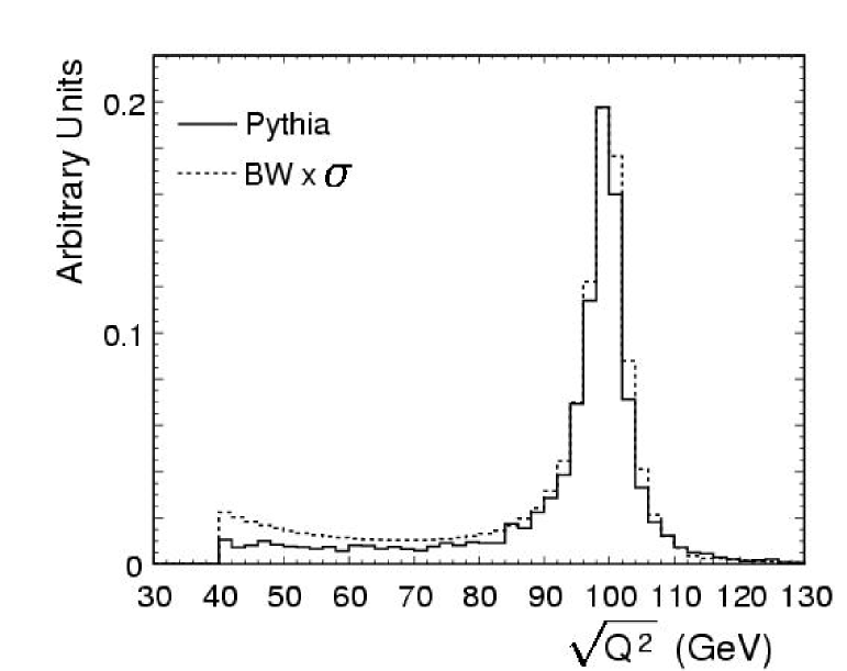
Figure 1: The figure shows the expected mass distribution of Higgs bosons produced directly at the Tevatron for $m_{A^{0}}~{}=~{}100$ GeV/c² and $\tan{\beta}~{}=~{}50$. We compare the output of Pythia 6.203 Sjostrand et al. (2001) with that obtained from the method described in this paper: folding in a simple relativistic Breit-Wigner distribution with the mass-dependent cross section calculation.

Therefore, scaling the Pythia differential distribution to the HIGLU one would underestimate the cross section because the off-shell events would not be accounted for.

To estimate the total cross section, we first retrieve the on-shell cross section as a function of mass in bins 1 GeV/$c^{2}$ wide using the HIGLU program. Then, the mass-dependent cross section is folded into a relativistic Breit-Wigner shape, with the width proportional to $Q^{2}$, from $Q^{2}=(40$ GeV$)^{2}$ to $Q^{2}=(200$ GeV$)^{2}$. For $m_{A^{0}}=100$ GeV/$c^{2}$ at $\tan{\beta}=50$, the MSSM cross-section for $A^{0}+h^{0}$ production is 122 pb.

The rate of Higgs boson production in the region of low $\sqrt{Q^{2}}$ is a source of significant uncertainty for the analysis, particularly at high mass and high $\tan{\beta}$. The low tail seen in Fig. 1 originates from a steeply falling cross section folded in with an increase in parton luminosities at small momentum transfer, folded in with a broad Higgs boson width. When we use the method outlined above to obtain a $Q^{2}$ dependent cross section, the size of the tail is bounded by those obtained when one generates events at the same parameter space point with Pythia and Isajet isa . We compare the result from the default Pythia output with that where we use the method above to estimate the systematic error from these low mass tails. At $m_{A^{0}}=100$ GeV/c² and $\tan{\beta}=50$, this uncertainty is $2\%$. At higher mass and higher $\tan{\beta}$, this systematic can become significant. At $m_{A^{0}}=140$ GeV/c², $\tan{\beta}=80$ the systematic is $30\%$.

It is important to properly model the boson $p_{T}$ for Higgs boson and $Z$ boson events because it impacts the relative rates of back-to-back and non-back-to-back events, and the di-tau mass resolution for the latter events. Figure 2 shows the $p_{T}$

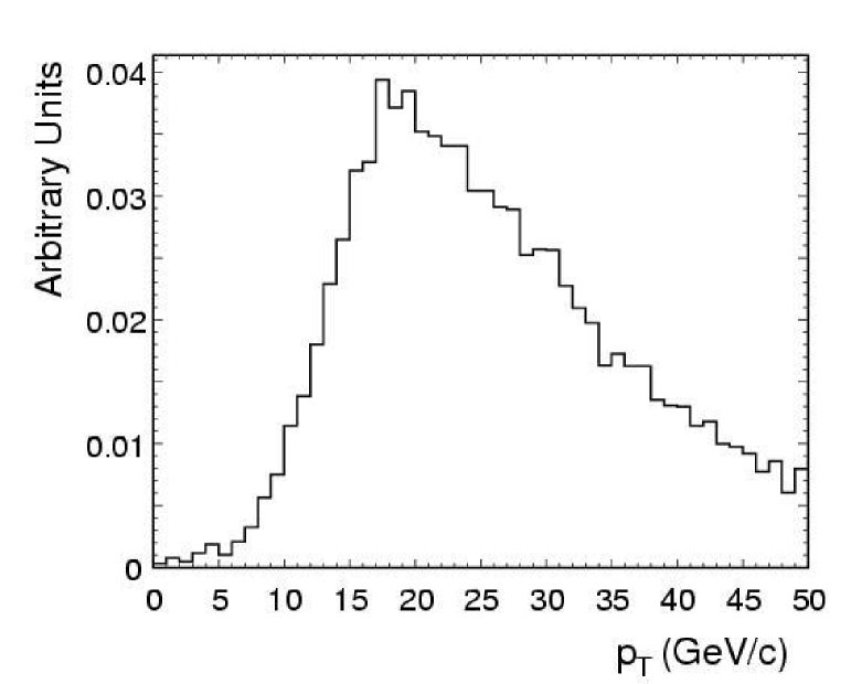
Figure 2: The $p_{T}$ of directly produced Higgs bosons with mass $m_{A}=100$ GeV after a $\sin{\Delta\phi}>0.3$ cut has been imposed.

distribution of the $A^{0}$ ($m_{A^{0}}=100$ GeV/c²) after the $\sin{\Delta\phi}>0.3$ cut is imposed, where $\Delta\phi$ is the angle between the taus in the transverse plane. We see that this cut is approximately equivalent to a cut of $p_{T}>15$ GeV/c imposed on the parent Higgs bosons.

In the high-$\tan{\beta}$ region of parameter space probed in this analysis, the direct-production process occurs predominantly through gluon fusion via a triangular bottom quark loop as in Fig. 3 (the direct production of SM Higgs bosons proceeds predominantly through a $t$ quark loop). In the default Pythia, the effect of the lighter quark mass in the fermion loop on the $p_{T}$ of Higgs bosons is not taken into account. To correct for this, we use Ellis et al. (1988) which performs a perturbative calculation for the differential cross section $d\sigma/dp_{T}$ to order $\alpha_{s}^{3}$ with a variable quark mass in the triangular loop. The perturbative calculation is valid in the region $p_{T}^{Higgs}\mathrel{\hbox to0.0pt{\lower 4.0pt\hbox{\hskip 1.0pt$\sim$}\hss}\raise 1.0pt\hbox{$>$}}15$ GeV/c. As has been pointed out, this cut is nearly equivalent to the requirement $\sin{\Delta\phi}>0.3$. We force agreement between the Higgs boson $p_{T}$ distributions in the region $p_{T}^{Higgs}>15$ GeV/c and the result of the program with a 5 GeV/c² $b$ quark in the fermion loop so that the resulting MC sample will have the proper efficiency for the $\sin{\Delta\phi}$ cut. To do this, we use a reweighting method known as the acceptance rejection MC method Eidelman et al. (2004).

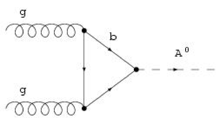
Figure 3: Feynman diagram of the direct production process. In the high-$\tan{\beta}$ region of parameter space, the gluon fusion process occurs predominantly through a triangular bottom quark loop.

The $p_{T}$ distributions for the $Z$ bosons from $Z/\gamma^{*}\rightarrow~{}e~{}e$ events has been measured by CDF in the region 66 GeV/c${}^{2}<M_{ee}<$116 GeV/c² Affolder et al. (2000a). $Z$ bosons from Pythia tend to have a lower average $p_{T}$ than the measured value. Therefore, we reweight both the $Z/\gamma^{*}~{}\rightarrow~{}\tau~{}\tau$ and $Z/\gamma^{*}\rightarrow ee$ samples to force agreement between the MC events and the measured spectrum. Only events that lie in the measured region are subject to rejection. This correction makes a significant difference in the relative rates of back-to-back and non-back-to-back events. Before the correction, 20% of the $Z$ events from Pythia are in the non-back-to-back region (here, defined by $p_{T}^{Z}>15$ GeV/c). After the correction, 26% of the events are in the non-back-to-back region.

CDF measured the cross section for $Z/\gamma^{*}\rightarrow ee$ in the same mass window as the $p_{T}$ distributions above, and reports this cross section to be 248 $\pm$ 11 pb Affolder et al. (2000a). Assuming universality, we scale the generated $Z\rightarrow\tau\tau$ sample to this cross section in the measured range.

Polarization effects, which impact the tau lepton kinematics, are properly taken into account with Tauola  Jadach et al. (1990). Simulated Higgs boson events tend to produce one tau with hard (high-$p_{T}$) visible decay products and one with soft visible decay products. Taus produced from $Z$ bosons are either both hard or both soft.

IV Event Selection and Efficiencies

The search is performed in a data sample of events collected using a high-$E_{T}$ electron trigger. In the following, we first describe the trigger system that an event must pass to enter this data sample, followed by a description of the electron and tau identification, and finally the event selection and mass reconstruction made at the analysis level.

IV.1 Trigger

A three-level trigger system was used to select events for  data storage Amidei et al. (1988) and the energy-dependent efficiency of these triggers has been measured Affolder et al. (2000b). At Level 1 (L1), the trigger requires at least one trigger tower with $E_{T}>8$ GeV in the CEM and the efficiency was measured to be 100% at the $10^{-3}$ level. At Level 2 (L2), the trigger requires one calorimeter cluster with $E_{T}~{}>~{}16$ GeV and the ratio of hadronic energy to electromagnetic energy ($E_{HAD}/E_{EM}$) to be less than 0.125. This cluster must be close in azimuthal angle to a track reconstructed in the trigger with $p_{T}>12$ GeV/c. The triggered sample contains 128,761 events. The efficiency of the L2 trigger for a good quality electron with $E_{T}>20$ GeV is $91\pm 2$%, measured from a $Z\rightarrow ee$ control sample. Signal events would pass this trigger approximately 20% of the time.

IV.2 Electron Identification

To improve the purity of the data, further cuts (listed in Table 1) are made on the candidate electron.

$E_{T}>20$ GeV

$p_{T}>13$ GeV/c

$E/p<1.5$

$Lshr<0.2$

$E_{HAD}/E_{EM}<0.05$

$|\Delta x|<1.5$ cm

$|\Delta z|<3.0$ cm

$\chi^{2}_{strip}<10.0$

$|z_{\mathrm{VTX}}-z_{e}|<5.0$ cm

$|z_{\mathrm{VTX}}|<60.0$ cm

Conversion Rejection

Fiducial cuts on the electron

Table 1: Cuts made offline to select the data sample used for the search. The electron identification variables are defined in Sec. IV.2.

These cuts are described in more detail in Abe et al. (1995a); we briefly summarize them here. We use $Z\rightarrow ee$ control samples to quantify the degree of agreement between the simulation and the data.

A candidate electron is first identified as a calorimeter cluster in the CEM. An electron cluster in the calorimeter is formed by merging seed towers (required to have $E_{T}>3$ GeV) with neighboring towers in $\eta$ ($E_{T}>0.1$ GeV required). To be called an EM cluster, $E_{T}>5$ GeV is required. Corrections are made to the energy of an EM cluster to compensate for variable response across each tower, tower-to-tower gain variations and time-dependent effects. A global correction to the energy scale is also imposed Abe et al. (1995b). These corrections are typically at the level of a few percent.

We require an electron candidate to have a CTC track pointing to an EM cluster. The highest $p_{T}$ track pointing to the cluster is the “electron track,” and is required to satisfy $p_{T}>13$ GeV/c. The measured direction of the track momentum sets the direction of the electron candidate.

We require that the ratio of the energy deposited in the EM calorimeter to the momentum of the electron track is not too large ($E/p<1.5$). Also, the lateral profile of the EM shower left by the electron tau candidate is required to be consistent with electron shower profiles as measured in test beam data ($Lshr<0.2$). The ratio of energy measured in the CHA to energy measured in the CEM ($E_{HAD}/E_{EM}$) is expected to be small for an electron from a tau decay; we require $E_{HAD}/E_{EM}<0.05$. In addition, the electron track projected to the plane of the CES must be close to a CES shower position: $|\Delta x|<1.5$ cm and $|\Delta z|<3.0$ cm. This reduces the background from charged pions produced in the neighborhood of neutral pions. We also confirm that the profile of the pulse heights produced by the electron shower across CES strips is consistent with electron test beam data: $\chi^{2}_{strip}<10.0$. The electron track is required to be consistent with a vertex that lies within 60 cm of the nominal collision point. Standard CDF fiducial cuts are made on the electron to ensure that the particle arrived at an instrumented region of the calorimeter with good response. We reject electron candidates which are consistent with having originated from a photon that converted to an electron-positron pair in the detector by removing candidates that leave a low-occupancy track in the VTX or that have a nearby opposite-sign track. The opposite-sign track must be within $90^{\circ}$ in $\phi$, separated in $r-\phi$ from the electron track by no more than 0.3 cm measured at the point where the tracks are parallel, satisfying $|\Delta\cot{\theta}|<0.06$ where $\Delta\cot{\theta}$ is the difference between the values of $\cot{\theta}$ for the two tracks. The electron tau candidate must be isolated in the calorimeter and in the tracking system. In the calorimeter, we use the standard CDF isolation variable defined by:

$$R_{\mathrm{iso}}=\frac{E^{\mathrm{cone}}-E^{\mathrm{cluster}}}{E^{\mathrm{cluster}}}$$ (1)

where $E^{cone}$ is the energy deposited in the calorimeter in a cone of $\Delta R~{}=~{}\sqrt{(\Delta\phi)^{2}+(\Delta\eta)^{2}}~{}=~{}0.4$ around the electron tau candidate and $E^{\mathrm{cluster}}$ is the energy of the EM cluster. We require $R_{\mathrm{iso}}<0.1$. We define $N_{iso}$ to be the number of tracks with $p_{T}>1$ GeV/c within $\Delta R<0.524$ of the EM cluster. This cone size is 30^∘, chosen to be the same as the outer radius of the isolation annulus used for identifying hadronic taus, described below. A track must originate within 5 cm of the electron track along the beam line to be counted in the isolation cone. We require that $N_{iso}=0$.

We require at least one EM cluster in the event with $E_{T}>20$ GeV passing the electron identification requirements just described. We refer to this as the electron tau ($\tau_{e}$) candidate. If there is more than one $\tau_{e}$ candidate in the event, we select the candidate with highest $E_{T}$.

We correct for inadequacies in simulation of electron identification variables by applying a scale factor of $0.869\pm 0.016$. The scale factor was determined using $Z/\gamma^{*}\rightarrow ee$ events and we have determined that is not $p_{T}$ dependent.

Since the vertex position affects the acceptance, we reweight the events to force agreement between the distribution of primary vertex positions from the simulation and that measured from the Run 1b data sample.

IV.3 Hadronic Tau Identification

$E_{T}>10$ GeV (jet)
$p_{T}>10$ GeV/c (track)
$N^{\mathrm{trks}}_{\mathrm{cone}}=1$ or $3$
$N^{\mathrm{trks}}_{\mathrm{ann}}=0$
Fiducial requirements
$|z_{\mathrm{VTX}}-z_{\tau_{h}}|<5.0$ cm
$|z_{\tau_{h}}|<60.0$ cm
$N^{\mathrm{ces}}_{\mathrm{cone}}<3$
$N^{\mathrm{ces}}_{\mathrm{ann}}=0$
$m_{\tau}<2.0$ GeV/c2
$\xi>0.15$
$I_{\phi-\phi}<0.1$ and $I_{\eta-\eta}<0.1$

Table 2: Cuts made offline for tau identification. These variables are defined in Sec. IV.3.

For taus coming from Higgs boson decays, the hadronic tau decay products will be collimated, with an angular deviation from the direction of the tau parent of no more than $\Delta\phi~{}\mathrel{\hbox to0.0pt{\lower 4.0pt\hbox{\hskip 1.0pt$\sim$}\hss}\raise 1.0pt\hbox{$<$}}~{}m_{\tau}/E_{\tau}$ which is $\sim 10^{\circ}$ for a typical $E_{\tau}\sim 10$ GeV. In nearly all cases, tau decay products will include 1 or 3 charged tracks and $\leq 2$ neutral pions, each decaying to two photons (all other decay modes have branching fractions of less than half of a percent).

The cuts used to select a hadronic tau are listed in Table 2. The $\tau_{h}$ identification cuts used here are based on those outlined in Abe et al. (1997b). The main differences are noted in what follows. The search for a $\tau_{h}$ begins with identifying a stiff track associated with a jet cluster. We require a track with $p_{T}>10$ GeV/c within $\Delta R<0.4$ of a jet cluster with $E_{T}>10$ GeV. The calorimeter cluster size is $\Delta R=0.4$. The track with the highest $p_{T}$ satisfying this requirement is called the tau seed. The $E_{T}$ cut is approximately 75% efficient for signal. The $p_{T}$ cut is approximately 65% efficient for signal while rejecting 80% of QCD jets (after the $E_{T}$ cut has already been imposed).

We make stringent fiducial requirements on the tau seed to ensure that the tau candidate’s energy is well measured. The track must be fully contained in the CTC and must pass additional fiducial cuts similar to those imposed on the electron candidate to ensure that it is not incident on an uninstrumented portion of the calorimeter. Also, to suppress fake track contamination, we require 0.5 GeV in the tower to which the track points. The seed track also must be within 5 cm of the same primary vertex ($|z_{\mathrm{VTX}}-z_{\tau_{h}}|<5.0$ cm) as the electron track.

In the neighborhood of the tau seed, two isolation regions are considered separately with different requirements made in each region: the $\Delta R<0.175$ cone and the $0.175~{}<~{}\Delta R~{}<~{}0.524$ annulus. In either isolation region, a track is a shoulder track if it is a good quality track with $p_{T}>1$ GeV/c. The seed track is included in the track counting in the $R<0.175$ cone.

For a true hadronically decaying tau, the number of tracks in the $\Delta R<0.175$ cone ($N^{\mathrm{trks}}_{\mathrm{cone}}$) is usually 1 or 3, so we require $N^{\mathrm{trks}}_{\mathrm{cone}}<4$. We additionally require the sum of the charges of the tracks in the cone to be $\pm 1$, and opposite to the charge of the electron. We expect the number of tracks in the annulus $0.175<R<0.524$ around the tau seed ($N^{\mathrm{trks}}_{\mathrm{ann}}$) to vanish in signal events, so we require $N^{\mathrm{trks}}_{\mathrm{ann}}~{}=~{}0$. These tracking isolation cuts retain approximately 80% of signal events and reject 70-80% of QCD jets.

The CES clustering algorithm used is the same as the one used in previous CDF analyses Abe et al. (1997b), with some modifications that improve tau purity and fake rejection. In particular, CES clusters were formed at a larger distance in $r-\phi$ from the seed track so that this information may be used for fake rejection. Also, a $\chi^{2}$ requirement that was used in previous CDF analyses to ensure the consistency of the CES cluster profile with electron test beam data was removed here to improve efficiency without a significant sacrifice in purity.

The algorithm forms CES clusters in the $\Delta R<0.6$ cone around the seed track by taking the highest energy strips (wires) in each calorimeter tower, in descending order, calling them seeds, and merging them with their nearest neighbors to form clusters 4 strips (6 wires) wide. To be a seed for a cluster, a strip (wire) must show a pulse height that surpasses 0.4 (0.5) GeV. The cluster position is defined as the position of the center strip or wire in the cluster. Pulse heights from strips and wires were corrected for $\eta-$ and $\phi-$dependent effects, measured from test-beam data. The energy of a CES cluster in a tower is the CEM energy of that tower, weighted by the energy deposited in the CES by that cluster compared to the energy deposited by all CES clusters in the tower. The predicted response in the CEM for a charged pion is subtracted from the energy in the tower impacted by the seed track. Wire clusters in the $r-\phi$ view are matched with strip clusters in the $z$ view with similar energies and merged into new clusters. The cluster position must not be consistent with coming from the seed track. It is rejected if $|\eta_{d}^{\mathrm{seed}}-\eta_{d}^{\mathrm{cluster}}|<0.03$ and either $|\phi^{\mathrm{seed}}-\phi^{\mathrm{cluster}}|<0.01$ or $|\phi^{tower\hskip 3.61371ptcenter}-\phi^{\mathrm{cluster}}|<0.01$ (the latter requirement is because the cluster position is assigned to the center of the tower in $\phi$ when no wire information is available).

A CES cluster must satisfy $E_{T}>1$ GeV to be counted as a shoulder cluster in either of the isolation regions. We call the number of CES clusters found in the isolation cone (annulus) $N^{\mathrm{ces}}_{\mathrm{cone}}$ ($N^{\mathrm{ces}}_{\mathrm{ann}}$) and require $N^{\mathrm{ces}}_{\mathrm{cone}}<3$ and $N^{\mathrm{ces}}_{\mathrm{ann}}=0$. In addition, the CES cluster energies in the cone measured as 3-component vectors are combined with the measured momenta of the tracks to compute a tau mass, $m_{\tau}$. We require $m_{\tau}<2.0$ GeV/c². The cuts on $N^{\mathrm{ces}}_{\mathrm{cone}}$, $N^{\mathrm{ces}}_{\mathrm{ann}}$ and $m_{\tau}$ give a combined efficiency for signal of approximately 95%. These three cuts additionally reject 30-50% of QCD jets.

As described above, a tau candidate is found to be isolated through a measurement of track and CES cluster multiplicities in the neighborhood of a seed track. We compare the isolation variables among $Z\rightarrow ee$, $Z\rightarrow\mu\mu$ and $Z\rightarrow\tau\tau$ simulation MC samples, and in $Z\rightarrow ee$ and $Z\rightarrow\mu\mu$ data control samples. In the $Z\rightarrow ee$ and $Z\rightarrow\mu\mu$ samples, both lepton candidates in the event mimic the tau seed in this analysis. We find good agreement between data and simulation, and between electron and muon samples, in the efficiencies of the isolation cuts. The isolation efficiencies from the simulated $Z\rightarrow\tau\tau$ MC sample also agrees with the data samples in the annulus around the tau seed (where no particles from tau decays are expected).

To reduce the impact of $Z/\gamma~{}\rightarrow~{}ee$ background on the sensitivity, we require $\xi>0.15$ where $\xi~{}=~{}E^{had}_{T}/\Sigma{p_{T}}$ Groer (1998). Here, $E^{had}_{T}$ is the hadronic energy of the tau jet cluster and $\Sigma{p_{T}}$ is the sum of the $p_{T}$ of all tracks with $p_{T}>1$ GeV/c within the cone $\Delta R<0.175$ centered on the jet direction.

Since the decay products of a hadronically decaying tau are highly collimated, a tau is expected to leave a narrow cluster of energy in the calorimeter. We cut on the $\phi-\phi$ and $\eta-\eta$ moments of the jet cluster associated with the hadronic tau candidate which are defined as follows:

$$I_{\phi-\phi}=\frac{\sum_{i}{E_{T}^{\hskip 3.61371pti}\cdot{(\phi_{i}-\phi_{0})}^{2}}}{\sum{E_{T}^{\hskip 3.61371pti}}}$$ (2)

$$I_{\eta-\eta}=\frac{\sum_{i}{E_{T}^{\hskip 3.61371pti}\cdot{(\eta_{i}-\eta_{0})}^{2}}}{\sum{E_{T}^{\hskip 3.61371pti}}}.$$ (3)

The sum is over calorimeter towers in the jet cluster, and $\phi_{0}$ and $\eta_{0}$ are the $E_{T}$ weighted center of the jet in the $\phi$ and $\eta$ directions. We require $I_{\phi-\phi}<0.1$ and $I_{\eta-\eta}<0.1$. These two cuts together reject approximately 30-45% of QCD jets.

Figure 4 shows the efficiency of the hadronic tau identification cuts from the simulation. We bin the efficiencies according to the visible transverse energy ($E_{T}$) from the tau at the generator level. The total efficiency plateaus near 55% for $E_{T}\mathrel{\hbox to0.0pt{\lower 4.0pt\hbox{\hskip 1.0pt$\sim$}\hss}\raise 1.0pt\hbox{$>$}}35$ GeV. For fiducial hadronic taus with $E_{T}>10$ GeV from $Z$ decays, the average efficiency of the tau identification cuts is 40%. $A\rightarrow\tau\tau$ events at $m_{A}=100$ GeV and $\tan{\beta}=50$ are also 40% efficient.

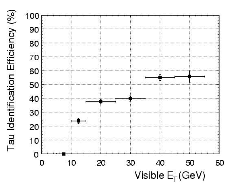
Figure 4: Efficiencies of the tau identification cuts applied to hadronic taus from $Z\rightarrow\tau\tau$ events .

IV.4 Additional Requirements

We make further cuts on the data sample to increase purity and further reject background. We require at most one recoil jet with $E_{T}>15$ GeV in the event. For further suppression of $Z\rightarrow ee$ background, we reject any event with two electrons or one electron and one track that have a reconstructed invariant mass $M_{ee}$ between 70 and 110 GeV/c², which removes 99% of $Z\rightarrow ee$ events while retaining 90% of signal events. We require a separation of the tau candidates in the transverse plane, $\Delta\phi>1.5$, where $\Delta\phi$ is the azimuthal angle between $\tau_{e}$ and $\tau_{h}$. This is nearly 100% efficient for signal rejecting 20% of non-tau backgrounds as measured from a background-dominated data sample.

To take advantage of the mass reconstruction technique, we divide the events into back-to-back and non-back-to-back samples. The full invariant mass of the di-tau system can be estimated only when the tau candidates are not back-to-back, as explained in more detail in Section IV E. The tau candidates are called back-to-back when $\sin\Delta\phi<0.3$, where $\Delta\phi$ is the azimuthal angle between $\tau_{e}$ and $\tau_{h}$. Note that $\sin\Delta\phi$ is the determinant of the system of equations which determine the di-tau mass, so when $\sin\Delta\phi\approx 0$, the solution is not unique.

The missing transverse energy in the event, denoted $\vec{E_{T}}/\hskip 7.22743pt$, is the opposite of the vector sum of the measured transverse energies of the event. For the non-back-to-back events, we use the magnitude and direction of $\vec{E_{T}}/\hskip 7.22743pt$ to derive the di-tau mass. First, we define corrected $E_{T}/\hskip 7.22743pt$ in the following way:

$$\vec{E_{T}}/\hskip 7.22743pt^{corr}=-\sum_{towers}{\vec{E_{T}}^{i}}-\sum_{muons}{\vec{p_{T}}^{j}}-\Delta\vec{E_{T}}^{ele}-\sum_{jets}\Delta\vec{E_{T}}^{i}.$$ (4)

The first term on the right side of the equation is a sum of the the transverse component of the energy deposited the calorimeter towers. The remaining terms improve the resolution by accounting for the momentum carried away by muons, energy corrections applied to the electron candidate, and jet energy corrections.

It is only necessary for the simulation to correctly model $\vec{E_{T}}/\hskip 7.22743pt^{corr}$ well in the region $p_{T}^{A,h,Z}>15$ GeV/c, since that is where the mass reconstruction is utilized. We confirm that the $\vec{E_{T}}/\hskip 7.22743pt^{corr}$ variable from the data is well modeled by the simulation using a sample of $Z\rightarrow ee$ events with $p_{T}^{Z}>15$ GeV/c.

IV.5 Di-tau Mass Reconstruction

Signal events contain neutrinos that escape CDF undetected. At hadron colliders, the resulting energy imbalance may only be determined in the transverse plane because the $z$-component of the total momentum of the interaction is unknown.

Nonetheless, the energy of the neutrinos from each tau decay, and thus the full mass of the di-tau system, may be deduced if (i) the tau candidates are not back-to-back in the transverse plane and (ii) the neutrino directions are assumed to be the same as their parent tausEllis et al. (1988); cms ; atl (a, b).

The contributions to the total missing energy from the leptonic and hadronic decays, denoted $E_{l}/\hskip 7.22743pt$ and $E_{h}/\hskip 7.22743pt$, are the solution to a system of two equations and two unknowns:

$$E_{l}/\hskip 7.22743pt\sin{\theta_{l}}\cos{\phi_{l}}+E_{h}/\hskip 7.22743pt\sin{\theta_{h}}\cos{\phi_{h}}=(E^{meas}/\hskip 23.12692pt)_{x}$$ (5)

$$E_{l}/\hskip 7.22743pt\sin{\theta_{l}}\sin{\phi_{l}}+E_{h}/\hskip 7.22743pt\sin{\theta_{h}}\sin{\phi_{h}}=(E^{meas}/\hskip 23.12692pt)_{y}$$ (6)

Here, $E^{meas}/\hskip 23.12692pt$ is the missing energy measured for the event and $\theta_{l,h}$ are the polar angles of the taus and $\phi_{l,h}$ are the azimuthal angles of the taus. The tau candidate directions are measured from the visible decay products.

The reason for the first of the two criteria for the mass technique outlined above is that when the tau candidates are back-to-back in the transverse plane, the reconstructed mass is not a good separating variable because there are many high mass solutions.

Some events may give negative solutions for $E_{l}/\hskip 7.22743pt$ and $E_{h}/\hskip 7.22743pt$. We require $E_{l,h}/\hskip 8.67204pt>0$ for the non-back-to-back events, which reduces non-di-tau backgrounds in this region. Figure 5 shows

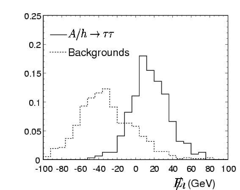
Figure 5: $E_{l}/\hskip 7.22743pt$ from simulated $A^{0}/h^{0}\rightarrow\tau\tau$ events compared to a background-dominated data sample.

$E_{l}/\hskip 7.22743pt$ from a background-dominated sample of the data compared to simulated $A^{0}/h^{0}\rightarrow\tau\tau$ events. The analogous distributions for $E_{h}/\hskip 7.22743pt$ are similar. The $E_{l,h}/\hskip 8.67204pt>0$ requirement is 55-60% efficient for signal, increasing with mass, while reducing non-di-tau background by approximately a factor of 10. When the di-tau mass is reconstructed as described next, this cut also improves the mass resolution.

We calculate the total reconstructed mass of the di-tau system using

$$\begin{split}m_{\tau\tau}^{2}&=m_{Z/h}^{2}=(p_{l}+p_{h})^{2}\\ &=2m_{\tau}^{2}+2(E_{l}/\hskip 7.22743pt+E_{l}^{vis})(E_{h}/\hskip 7.22743pt+E_{h}^{vis})(1-\cos{\psi})\\ \end{split}$$ (7)

where $p_{l}$ and $p_{h}$ are the 4-momenta of each tau, and $E_{l}$ and $E_{h}$ represent the total energy of each tau. $E_{l}^{vis}$ and $E_{h}^{vis}$ represent the energy left by their visible decay products. The $\psi$ is the 3-dimensional angle between the two taus. The missing energies $E_{l}/\hskip 7.22743pt$ and $E_{h}/\hskip 7.22743pt$ are the solutions to Eqs. 5 and  6.

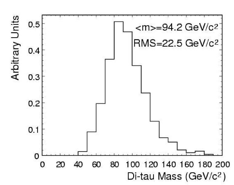
Figure 6: Di-tau mass distribution as modeled by Pythia 6.203 and the CDF detector simulation with parameters $m_{A}=100$ GeV and $\tan{\beta}=50$. A $\sin(\Delta\phi)>0.3$ cut has been imposed.

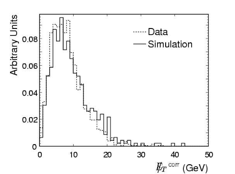
Figure 7: Corrected missing energy as measured from a $Z\rightarrow ee$ data control sample, only for events where $p_{T}^{Z}>15$ GeV/c.

Figure 6 shows the di-tau mass distribution reconstructed from signal events for the parameter point $m_{A^{0}}=100$ GeV/c² and $\tan{\beta}=50$, for which the $A^{0}$ or $h^{0}$ particle has an inherent width of 5.7 GeV/c². The contribution from the calorimeter resolution may be qualitatively seen from Fig. 7, since $Z\rightarrow ee$ events would have a small $E_{T}/\hskip 7.22743pt$. The remaining contribution to the width of the di-tau mass distribution comes from the approximations that are needed to implement the technique, listed above.

Cut	No. Events
Triggered Events	128,761
Electron ID & $N_{iso}=0$	58534
$Z$ Rejection	50943
$N_{jets}<3$	50415
Fiducial Jet	9097
Jet $E_{T}>10$ GeV/$c^{2}$	6478
$\geq 1$ Tau Seed	1265
$\Delta\phi>1.5$	1117
	$\sin{\Delta\phi}<0.3$	$\sin{\Delta\phi}>0.3$
$\sin{\Delta\phi}$	510	607
# Tracks	189	146
Elect. Reject	98	93
$m_{\tau}<2$ GeV/$c^{2}$	93	84
# CES	80	72
Jet Width	64	54
$|Q|=1$	48	39
Opp. Sign	39	28
$E_{l}/\hskip 7.22743pt>0$, $E_{h}/\hskip 7.22743pt>0$	NA	8

Table 3: A summary of the cuts imposed and the number of events remaining in the data sample after each successive cut.

Cut	Efficiency (%)
	$Z\rightarrow\tau\tau$		$A^{0}+h^{0}\rightarrow\tau\tau$
BR($\tau\rightarrow e$)	32.5		32.5
$|\eta_{e}|<1.2$	19.8		26.5
Electron ID & $N_{iso}=0$	35.6		37.5
L2 Trigger	90.8		91.0
$Z$ Rejection	93.3		90.3
$N_{jets}<3$	97.7		96.4
Fiducial Jet	35.3		40.6
Jet $E_{T}>10$ GeV	89.4		90.3
$\geq 1$ Tau Seed	64.0		65.1
$\Delta\phi>1.5$	100.0		100.0
	$\sin{\Delta\phi}<0.3$		$\sin{\Delta\phi}>0.3$
$\sin{\Delta\phi}$	84.1	15.9	80.7	19.4
# Tracks	84.3	85.9	82.3	83.0
Elect. Reject	95.5	96.0	95.2	95.0
$m_{\tau}<2$ GeV	98.5	98.6	98.5	98.4
# CES	97.0	96.6	96.9	97.7
Jet Width	92.2	92.5	92.7	92.0
$|Q|=1$	93.1	92.9	92.7	92.8
Opp. Sign	99.8	100.0	99.8	100.0
$E_{l}/\hskip 7.22743pt>0$, $E_{h}/\hskip 7.22743pt>0$	NA	56.8	NA	58.0

Table 4: Efficiency of each cut imposed on $Z\rightarrow\tau\tau$ and $A^{0}+h^{0}\rightarrow\tau\tau$ simulated events. Back-to-back and non-back-to-back events are denoted $\sin{\Delta\phi}<0.3$ and $\sin{\Delta\phi}>0.3$, respectively.

Table III summarizes the cuts that we impose and the number of events remaining in the sample after each cut. Table IV summarizes the efficiency of each cut on the $Z\rightarrow\tau\tau$ and $A^{0}+h^{0}\rightarrow\tau\tau$ simulated events.

V Backgrounds

The backgrounds can be classified into two categories: physics and instrumental backgrounds. The former includes $Z\rightarrow\tau\tau$ and $Z/\gamma^{*}\rightarrow ee$. The latter fall into three categories: events containing a conversion pair and a recoil jet, $W(\rightarrow e\nu)$+jets events and events containing a jet that fakes an electron. All of these contain a fake hadronic tau. We model signal and physics backgrounds using Pythia Monte-Carlo and the CDF detector simulation Sjostrand et al. (2001).

We estimate the rate of all fake tau contributions combined instead of estimating each source of fakes separately. This way, we do not rely on modeling of jets, nor on limited control samples for each separate background. We estimate the number of fakes expected to pass all of the cuts using the fake rate technique described next.

We use five different control samples from CDF data to measure the rate at which a jet fakes a hadronic tau by passing the tau identification cuts for this analysis. They are: (i) a sample dominated by events where a photon produced an electron pair, (ii) a sample dominated by $W(\rightarrow e\nu)$+jets, (iii) another dominated by $W(\rightarrow\mu\nu)$+jets and two samples of events collected using inclusive triggers with a jet satisfying (iv) $E_{T}>20$ GeV and (v) $E_{T}>50$ GeV. The first three are classified as lepton samples and the latter two are jet samples.

A fake rate is defined as the probability that a jet passes the hadronic tau identification requirements as described in Sec. IV.3. For all data control samples, we measure the fake rates in bins defined by the $E_{T}$ of the jet associated with the tau candidate. Figure 8 shows the fake

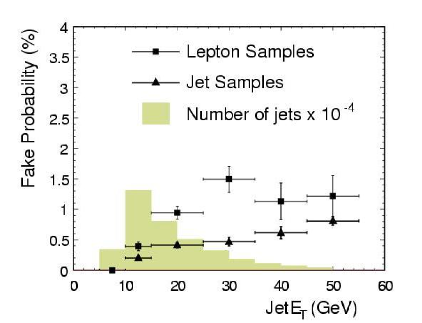
Figure 8: Hadronic tau fake rates as measured in the lepton control samples compared with that measured in the jet control samples.

rates measured from all three lepton samples combined and from both jet samples combined. We measure fake rates less than about 1% from the jet samples, which are as good as in previous tau analyses Groer (1998). We find that the fake rates measured from the lepton samples are approximately a factor of 2 higher than from the jet samples. Two of the lepton samples are dominated by W+jets events where the recoil jet comes from a quark; quark jets are narrower, have lower multiplicity and are thus more likely to pass the tau identification cuts qua . Still, the reason for this difference is not definitively understood. Since the analysis is performed in a lepton sample, we use the fake rates measured from the lepton samples as the central value and the difference between the rates from the two different types of samples as a systematic uncertainty. The histogram in Fig. 8 shows the $E_{T}$ distribution of jets in the data sample just before tau identification cuts are applied. The fake rates are folded into this $E_{T}$ distribution to predict the rate of fake tau background.

We find that fake taus from the $W$+jets samples are opposite-sign from the lepton in the event (67.1 $\pm$ 3.0)% of the time. This is due to a correlation between the W and the recoiling quark. The isolation cut enhances this correlation due to charge conservation. In the conversion sample, the opposite-sign requirement is consistent with being 50% efficient. We take the central value of the efficiency for the opposite-sign cut to be the average of the two ($(67.1+50)/2=58.6\%$) and equally likely to be anywhere between 50.0% and 67.1%.

To estimate the number of fake taus expected to pass all of the cuts, we use the data sample with the following cuts removed: (i) tau ID cuts (ii) the opposite sign requirement and (iii) $E/_{\tau_{1},\tau_{2}}>0$. Then, we fold in the measured fake rates with the $E_{T}$ spectrum of jets. There are 6478 events that pass these cuts and which contain at least one jet passing the fiducial cuts. We apply our measured fake rates to 6972 jets from these events. For each jet, we give it a weight equal to the fake rate measured for its $E_{T}$. We expect 21.0 $\pm$ 12.1 back-to-back and 29.8 $\pm$ 16.8 non-back-to-back for a total of 50.8 $\pm$ 29.0 fakes before the remaining cuts are applied.

We apply two final cuts to improve the purity of the sample. We apply the opposite sign requirement, taking the efficiency to be 58.6%. Including the systematic error from this cut, we expect 10.5 $\pm$ 6.0 back-to-back and 14.9 $\pm$ 8.5 non-back-to-back events at this stage. The final cut is the $E/_{\tau_{1},\tau_{2}}>0$ cut applied to the non-back-to-back events only. This is measured from the same background-dominated sample, subtracting out $Z\rightarrow\tau\tau$ and $Z\rightarrow ee$ contamination. We find that this cut removes 89.0% of the fake tau background. This brings the number of predicted non-back-to-back events with a fake tau to 1.6. Added to the back-to-back events, we expect 1.6 + 10.5 = 12.1 events containing a fake hadronic tau to pass the analysis cuts. At each stage of this estimation, we account for the 10%-level $Z\rightarrow\tau\tau$ and $Z\rightarrow ee$ contamination of the background-dominated sample.

VI Summary of Systematic Uncertainties

In Tab. V , we summarize the systematics on the backgrounds and signal. $Z\rightarrow ee$ is not included in the table because the expected rate is based on a low number of background events. We expect 0.6 $\pm$ 0.3 $Z\rightarrow ee$ events in the counting experiment. The systematics on the fake tau background are described in Sec. V.

The error on the Run 1b luminosity at CDF is 4.1% Cronin-Hennessy et al. (2000). The systematic error on the electron identification cuts is 1.8%, as noted in Sec. IV. This error comes from the limited size of the $Z\rightarrow ee$ sample used for comparing the simulation with data. The systematic error due to the modeling of the trigger efficiency is obtained by moving the parameters in the energy and $\eta$-dependent efficiency by one standard deviation in each direction and measuring the effect on the total efficiency of all cuts. This systematic is 1.6% (1.7%) for $A^{0}/h^{0}\rightarrow\tau\tau$ ($Z\rightarrow\tau\tau$).

The one systematic uncertainty on the yield of signal events that varies significantly with the mass of the Higgs boson is the uncertainty on the cross section due to the low $\sqrt{Q^{2}}$ tail. Here are the systematic uncertainties due to this effect for each parameter space point considered in this note: $m_{A^{0}}=100$ GeV/c², $\tan{\beta}=50$, 0.5%; $m_{A^{0}}=110$ GeV/c², $\tan{\beta}=50$, 2.5%; $m_{A^{0}}=120$ GeV/c², $\tan{\beta}=50$, 3.5%, $m_{A^{0}}=140$ GeV/c², $\tan{\beta}=50$, 7.2%; $m_{A^{0}}=140$ GeV/c², $\tan{\beta}=80$, 21.3%. The systematic uncertainty on the $Z$ production cross section is $1.7\%$ based on the CDF measurement Affolder et al. (2000c).

By studying isolated pions, we have shown that the detector simulation overestimates the width of jets from charged pions, and thus underestimates the efficiency of the cut on jet width on the hadronic tau candidates. Therefore, we take the efficiency for that cut to be the average of the simulated efficiency and 100%, which is (100.0+92.2)/2 = 96.1%. The systematic error on this cut is half the difference between the efficiency from simulation and 100%, which is (100.0-92.2)/2 = 3.9%. The electron rejection cut applied to the hadronic tau candidate is not modeled sufficiently for hadronic decays. The same study of isolated pions previously mentioned showed that the hadronic energy deposited by charged pions is underestimated by the simulation, so that the efficiency of this cut is underestimated. We take the efficiency to be the average of the efficiency from simulation for hadronic taus and 100%, which is (100.0+95.5)/2 = 97.8%. The systematic error on this cut is half the difference between the simulated efficiency and 100%, which is (100.0-95.5)/2 = 2.2%. We obtain the jet energy scale systematic by varying the energies of all of the jets (except those identified as electrons) up and down by 5%. The resulting systematic error is 1.0% (1.2%) for $A^{0}/h^{0}\rightarrow\tau\tau$ ($Z\rightarrow\tau\tau$). There is a systematic uncertainty attributed to the tau fake rates since we measured different rates in lepton and jet samples. We set this systematic uncertainty to the the difference between the fake rates measured in the two types of samples; it is the dominant systematic error at 57.1%.

systematic uncertainty	$A^{0}/h^{0}\rightarrow\tau\tau$	$Z\rightarrow\tau\tau$	Fakes
	(%)	(%)	(%)
luminosity	4.1	4.1	–
cross section	0.5	1.7	–
electron ID	1.8	1.8	–
sample dependence of fake rates	–	–	57.1
opposite sign	–	–	14.7
jet width	3.9	3.9	–
jet energy scale	1.0	1.2	–
trigger efficiency	1.6	1.7	–
electron rejection	2.2	2.2	–
total error (%)	6.7	7.0	NA

Table 5: Summary of systematic uncertainties on the counting experiment for the final cuts. Here we refer to Higgs boson events corresponding to the parameter space point $m_{A^{0}}=100$ GeV, $\tan{\beta}=50$. All systematic uncertainties are quoted as a percentage of the total number of events observed after all cuts are applied. $Z\rightarrow ee$ is not included in the table because it is based on a low number of MC events. The errors attributed to the rate of fake taus are not both Gaussian, and are therefore not added in quadrature. See the text.

VII Results

We set limits on direct $A^{0}/h^{0}$ production in the MSSM based on a counting experiment using events from both the back-to-back and non-back-to-back samples. Then we show the limits achieved from a binned likelihood fit to the di-tau mass distribution from the non-back-to-back events alone. Our nominal limits come from the counting experiment utilizing both back-to-back and non-back-to-back events.

VII.1 All Events

We plot the track multiplicity of the tau candidates after imposing all of the analysis cuts except the following cuts: i) $|\sum{Q_{i}}|=1$, ii) $N^{trks}_{cone}<4$ and iii) the opposite sign requirement. Figure 9 shows the number of tracks in the 0.175 cone around the tau seed in the hadronic tau candidate in the event. We expect 78.2 events to appear in this plot and we observe 81.

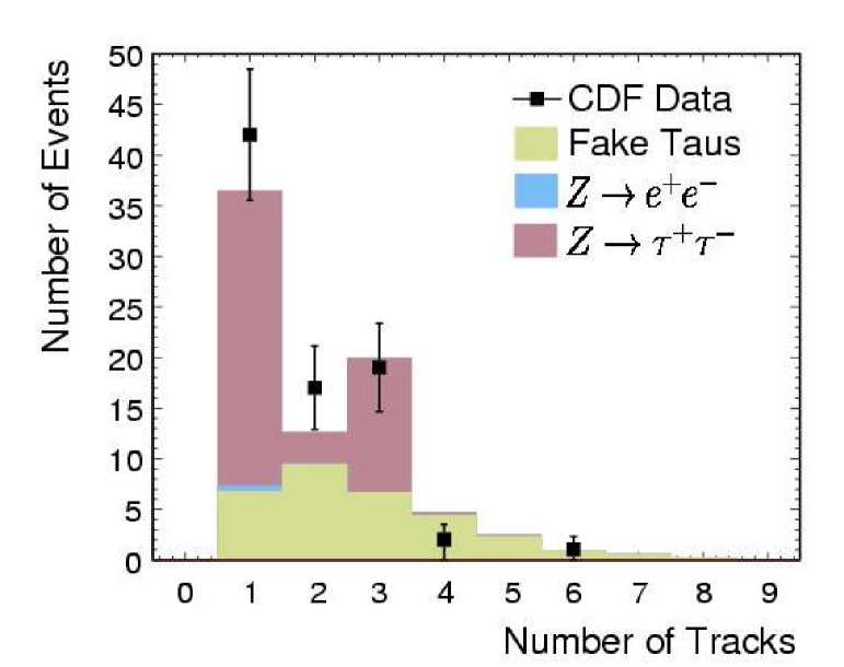
Figure 9: Track multiplicity distribution for the counting experiment, but without the $|Q|=1$, opposite sign and $N^{trks}_{cone}<4$ requirements.

Table 6 lists the number of events expected of each background type. The data and the prediction show good agreement at each stage. Of the 47 final observed events, 35 are 1-track and 12 are 3-track. The final three cuts reduce the fake background in these two bins by nearly a factor of 2 compared to that shown in Fig. 9 and leaves the $Z\rightarrow\tau\tau$ background in those bins virtually unchanged.

	$Z\rightarrow\tau\tau$	$Z\rightarrow ee$	Fake Taus	Total	Obs.
All cuts but
$|Q|=1$, Opposite Sign	46.1	0.56	31.5	78.2	81
$|Q|=1$,# Tracks$<4$	42.4	0.56	20.2	63.1	61
Opposite Sign	42.4	0.56	11.8	54.8	47

Table 6: Number of each background type expected, in the track multiplicity plot and after subsequent cuts are imposed, compared with the number observed.

VII.2 Non-Back-to-Back Events

Figure 10 shows the track multiplicity distribution for the non-back-to-back events only (since we will be performing the di-tau mass reconstruction on these events). These events have passed the $E_{l,h}/\hskip 8.67204pt>0$ requirement but the $|Q|=1$, opposite sign, and $N^{trks}_{cone}<4$ requirements have not been imposed. We expect 9.2 events to appear in the plot and we observe 15. The probability for the disagreement between data and the prediction to be equal to or more than what was observed is 3.2%.

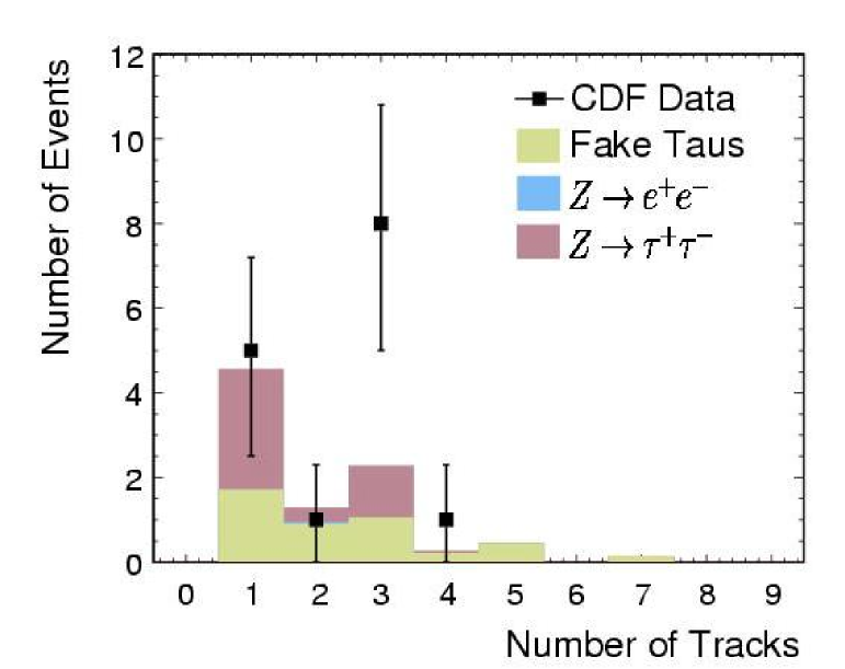
Figure 10: Track multiplicity distribution for the non-back-to-back events with the $E_{l,h}/\hskip 8.67204pt>0$ requirement, but without the $N^{trks}_{cone}<4$, $|Q|=1$ and opposite sign requirements.

Table 7 lists the number of events expected of each background type in Fig. 10 including non-back-to-back events only. We also show the expectation compared to the observed after the subsequent cuts are imposed. The final 8 events contain 5 1-track events and 3 3-track events.

	$Z\rightarrow\tau\tau$	$Z\rightarrow ee$	Fake Taus	Total	Obs.
All cuts but
$|Q|=1$, Opposite Sign	4.4	0.05	4.5	9.2	15
$|Q|=1$,# Tracks$<4$	4.1	0.05	3.0	7.1	13
Opposite Sign	4.1	0.05	1.7	5.9	8

Table 7: Number of each background type expected, in the track multiplicity plot and after subsequent cuts are imposed, compared with the number observed. Only non-back-to-back events are included.

VII.3 Limits

The numbers of observed events do not show an excess above the standard model expectation for background processes. Therefore, we set a limit on the product of the cross section and branching ratio of $A^{0}/h^{0}\rightarrow\tau\tau$ ($\sigma\cdot$ BR) at 95% confidence level. We take the branching ratio to be 9% for all parameter space points considered. We use a Bayesian method with a flat prior based on a likelihood that is smeared to account for systematic errors.

Table 8 shows the predicted and observed upper limits on $\sigma\cdot$ BR for $A^{0}/h^{0}$ production in the MSSM as a function of $m_{A^{0}}$ at $\tan{\beta}=50$. For $m_{A^{0}}=100$ GeV/c², $\tan{\beta}=50$ in the MSSM, the expected limit is 23.4 signal events, corresponding to 102 pb. Since we observed slightly fewer events than we expected, the observed limits are better than our expected limits. The observed limit is 77.9 pb. The limits on the $\sigma\cdot$ BR improve with increasing mass since the efficiency improves, but we are less sensitive to the MSSM theory at higher mass due to the steeply falling predicted cross section.

Mass	$\sigma\cdot$BR	Eff.	95% CL	95% CL
GeV/c2	pb	%	Exp. (pb)	Obs. (pb)
100	11.0	0.78	102	77.9
110	5.8	0.91	87.4	67.2
120	4.0	0.97	82.3	63.0
140	1.6	1.1	75.2	57.9

Table 8: 95% CL limits vs. $m_{A^{0}}$ for $\tan{\beta}=50$. The first two columns are the mass of the Higgs boson for each parameter point and the corresponding theoretically predicted $\sigma\cdot$ BR.

The cross section for producing $A^{0}/h^{0}$ in the MSSM scales with $(\tan{\beta})^{2}$. The sensitivity does not improve by that same factor, however, because the Higgs boson width scales as $(\tan{\beta})^{2}$, and the tail at low $\sqrt{s}$ also becomes more prominent with increasing $\tan{\beta}$, increasing the systematic error due to the uncertainty in the cross section in this region. At $m_{A^{0}}=140$ GeV/c² and $\tan{\beta}=80$, the uncertainty on the efficiency of the selection of Higgs boson events due to this low mass tail is 20%, compared to 7.2% at $m_{A^{0}}=140$ GeV/c², $\tan{\beta}=50$. Also, both effects bring down the efficiency at higher $\tan{\beta}$: at $m_{A^{0}}=140$ GeV/c² and $\tan{\beta}=80$, the efficiency is similar to the efficiency at a lower mass point: $m_{A^{0}}=110$ GeV/c², $\tan{\beta}=50$. Table 9 shows the limits for two different values of $\tan{\beta}$ for $m_{A^{0}}=140$ GeV/c². These limits are also summarized in Figure 11.

$\tan{\beta}$	$\sigma\cdot$ BR	Eff.	95% CL	95%CL
	pb	%	Exp. (pb)	Obs. (pb)
50	17.8	1.1	75.2	57.9
80	65.9	0.85	118	90

Table 9: 95% CL limits vs. $\tan{\beta}$ for $m_{A^{0}}=140$ GeV/c². All limits are quoted in pb. The efficiencies shown do not include branching ratios. The first two columns are the mass of the Higgs boson for each parameter point and the corresponding theoretically predicted $\sigma\cdot$ BR.

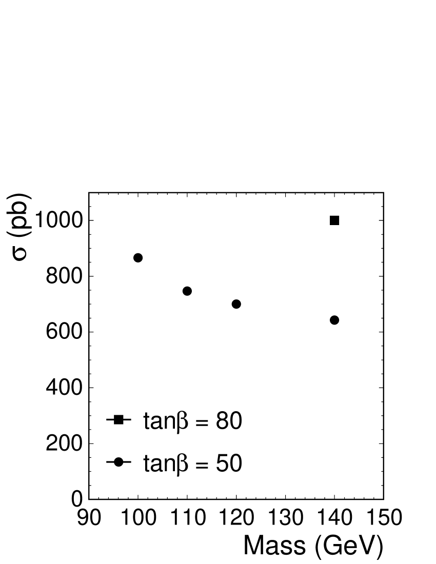
Figure 11: Summary of limits achieved in this analysis on the cross section for directly produced Higgs bosons for each parameter space point considered.

In the non-back-to-back region, after all cuts are applied, we expect 5.9 events and observe 8. Figure 12 shows the di-tau mass distribution for these 8 events compared with the expectation. In this region, limits are obtained by fitting the mass distribution using a binned likelihood, with 14 bins between 60 GeV/c² and 200 GeV/c² in di-tau mass.

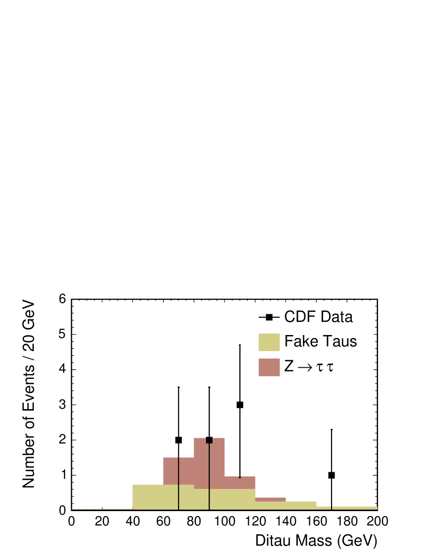
Figure 12: Di-tau mass reconstruction for events in the non-back-to-back region. It is compared with the background prediction, shown for fake tau backgrounds and then the $Z\rightarrow\tau\tau$ background added to it. The negligible contribution from $Z\rightarrow ee$ is not shown.

Table X shows the upper limits on the MSSM $\sigma\cdot$ BR obtained from the binned likelihood for four different values of $m_{A^{0}}$ for $\tan{\beta}=50$. At $m_{A^{0}}=100$ GeV/c², where the Higgs boson mass is nearly on top of the $Z$ mass, the mass reconstruction is less effective than at higher masses, so the expected limit from the binned likelihood in the non-back-to-back region is approximately 2.4 times worse than the expected limit from the counting experiment without the non-back-to-back requirement. At $m_{A^{0}}=140$ GeV/c², which is approximately 2 RMS away from the $Z$ in the di-tau mass variable, the expected limit from the binned likelihood using the non-back-to-back events is 2.1 times worse than the counting experiment limit, showing a modest improvement, but still not coming close to the expected limit from the counting experiment. With more data collected in Run 2, the power of the di-tau mass reconstruction technique will improve. Table XI shows the upper limits obtained from the binned likelihood for two different values of $\tan{\beta}$.

Mass	$\sigma\cdot$ BR	Eff.	95% CL	95% CL
GeV/c2	pb	%	Exp. (pb)	Obs. (pb)
100	11.0	0.093	247	395
110	5.8	0.10	218	379
120	4.0	0.105	199	363
140	1.6	0.12	158	309

Table 10: 95% CL limits vs. $m_{A^{0}}$ for $\tan{\beta}=50$, using the binned likelihood. The first two columns are the mass of the Higgs boson for each parameter point and the corresponding theoretically predicted $\sigma\cdot$ BR.

$\tan{\beta}$	$\sigma\cdot$ BR	Eff.	95% CL	95% CL
	pb	(%)	Exp. (pb)	Obs. (pb)
50	1.6	0.12	158	309
80	5.9	0.09	274	533

Table 11: 95% CL limits vs. $\tan{\beta}$ for $m_{A^{0}}=140$ GeV/c², using the binned likelihood. All limits are quoted in pb. The efficiencies shown do not include branching ratios. The first two columns are the mass of the Higgs boson for each parameter point and the corresponding theoretically predicted $\sigma\cdot$ BR.

VIII Conclusions

We have performed a search for directly produced Higgs bosons decaying to two taus where one tau decays to an electron and the other hadronically in Run 1b data at CDF. This is the first Higgs boson search based on the di-tau final state at a hadron collider. The number of events that pass all of the cuts is consistent with the background expectation. This agreement between data and background demonstrates our capability to reconstruct $Z\rightarrow\tau\tau$ final states, the irreducible background for this analysis. At a benchmark parameter space point, $m_{A^{0}}=100$ GeV/c² and $\tan{\beta}=50$, we are sensitive to a $\sigma\cdot$ BR of 102 pb compared to the 11.0 pb predicted in the MSSM. The observed limit at this parameter space point is 77.9 pb.

A di-tau mass reconstruction is performed for tau candidate pairs which are not back-to-back, for the first time with hadron collider data. The modest sensitivity that one gains from a limit binned in mass is not nearly enough to make up for the hit in efficiency taken when only non-back-to-back events are considered. At $m_{A^{0}}=100$ GeV/c², the binned mass limit at $\tan{\beta}=50$ from non-back-to-back events alone is 395 pb. At $m_{A^{0}}=140$ GeV/c², $\tan{\beta}=50$, the binned mass limit is 309 pb, showing a modest improvement as the Higgs boson mass is moved away from the $Z$ mass.

While this search does not have the sensitivity to the Standard Model Higgs boson that prior searches using decays to pairs of $b$ quarks, it lays the groundwork for similar analysis to be performed by future experiments. The di-tau mass reconstruction technique demonstrated here may also be useful for searches for other processes where a Higgs boson is produced with a recoil, such as $Hb$ or $Hb\bar{b}$.

IX Acknowledgements

We thank the Fermilab staff and the technical staffs of the participating institutions for their vital contributions. This work was supported by the U.S. Department of Energy and National Science Foundation; the Italian Istituto Nazionale di Fisica Nucleare; the Ministry of Education, Science and Culture of Japan; the Natural Sciences and Engineering Research Council of Canada; the National Science Council of the Republic of China; the A.P. Sloan Foundation.

References

- Nilles (1984) H. Nilles, Phys. Rep. 110, 1 (1984).
- Haber and Kane (1985) H. Haber and G. Kane, Phys. Rep. 117, 75 (1985).
- Barbieri (1988) R. Barbieri, Riv. Nuovo Cim. 11 4, 1 (1988).
- J. Ellis (1991) F. Z. J. Ellis, G. Ridolfi, Phys. Lett. B257, 83 (1991).
- Y. Okada (1991) T. Y. Y. Okada, M. Yamaguchi, Prog. Theor. Phys. 85, 1 (1991).
- Haber and Hempfling (1991) H. Haber and H. Hempfling, Phys. Rev. Lett. 66, 1815 (1991).
- (7) LEP Higgs Working Group, Searches for the neutral Higgs bosons of the MSSM: Preliminary combined results using LEP data collected at energies up to 209 GeV, hep-ex/0107030 (2001).
- Affolder et al. (2001) T. Affolder et al. (CDF Collaboration), Phys. Rev. Lett. 86, 4472 (2001).
- Acosta et al. (2004) D. Acosta et al. (CDF Collaboration), Phys. Rev. Lett. 92, 051803 (2004).
- Abe et al. (1997a) F. Abe et al. (CDF Collaboration), Phys. Rev. Lett. 78, 2906 (1997a).
- Abe et al. (1988) F. Abe et al. (CDF Collaboration), Nucl. Instrum. Methods Phys. Res. A 271, 387 (1988).
- Abe et al. (1994) F. Abe et al. (CDF Collaboration), Phys. Rev. D 50, 2966 (1994).
- Amidei et al. (1994) D. Amidei et al., Nucl. Instrum. Methods Phys. Res. A 350, 73 (1994).
- Azzi et al. (1995a) P. Azzi et al., Nucl. Instrum. Methods Phys. Res. A 360, 137 (1995a).
- Balka et al. (1988) L. Balka et al., Nucl. Instrum. Methods Phys. Res. A 268, 50 (1988).
- Hahn et al. (1988) S. R. Hahn et al., Nucl. Instrum. Methods Phys. Res. A 267, 351 (1988).
- Yasuoka et al. (1988) K. Yasuoka et al., Nucl. Instrum. Methods Phys. Res. A 267, 315 (1988).
- Wagner et al. (1988) R. G. Wagner et al., Nucl. Instrum. Methods Phys. Res. A 267, 330 (1988).
- Devlin et al. (1988) T. Devlin et al., Nucl. Instrum. Methods Phys. Res. A 267, 24 (1988).
- Azzi et al. (1995b) P. Azzi et al., Nucl. Instrum. Methods Phys. Res. A 360, 137 (1995b).
- Sjostrand et al. (2001) T. Sjostrand et al., Computer Physics Commun. 135, 238 (2001).
- (22) M. Spira, hep-ph/9510347 (1995).
- (23) H. Baer, F. Paige, S. Protopopescu, and X. Tata, hep-ph/0001086 (2000).
- Ellis et al. (1988) R. Ellis, I. Hinchliffe, M. Soldate, and J. V. D. Bij, Nucl. Phys. B 297, 221 (1988).
- Eidelman et al. (2004) S. Eidelman et al., Phys. Lett. B 592, 1 (2004).
- Affolder et al. (2000a) A. Affolder et al. (CDF Collaboration), Phys. Rev. Lett. 84, 845 (2000a).
- Jadach et al. (1990) S. Jadach, J. H. Kuhn, and Z. Was, Comput. Phys. Commun. 64, 275 (1990).
- Amidei et al. (1988) D. Amidei et al., Nucl. Instrum. Methods Phys. Res. A 269, 68 (1988).
- Affolder et al. (2000b) T. Affolder et al. (CDF Collaboration), Phys. Rev. Lett. 84, 845 (2000b).
- Abe et al. (1995a) F. Abe et al. (CDF Collaboration), Phys. Rev. D52, 2624 (1995a).
- Abe et al. (1995b) F. Abe et al. (CDF Collaboration), Phys. Rev. D52, 4784 (1995b).
- Abe et al. (1997b) F. Abe et al. (CDF Collaboration), Phys. Rev. Lett. 79, 357 (1997b).
- Groer (1998) L. Groer, Ph.D. thesis, Rutgers University (1998).
- (34) CMS Technical Proposal (1994), 191-192.
- atl (a) ATLAS Detector and Physics Performance. Technical Design Report. Vol. 1, CERN-LHCC-99-14.
- atl (b) ATLAS Detector and Physics Performance. Technical Design Report. Vol. 2, CERN-LHCC-99-15.
- (37) D. Acosta et al. (CDF Collaboration), FERMILAB-PUB-04-113-E.
- Cronin-Hennessy et al. (2000) D. Cronin-Hennessy, A. Beretvas, and P. F. Derwent (CDF Collaboration), Nucl. Instrum. Meth. A443, 37 (2000).
- Affolder et al. (2000c) T. Affolder et al. (CDF Collaboration), Phys. Rev. Lett. 84, 845 (2000c).