Averages of $b$-hadron Properties
as of Winter 2005

Abstract

This article reports world averages for measurements on $b$-hadron properties obtained by the Heavy Flavor Averaging Group (HFAG) using the available results as of winter 2005 conferences. In the averaging, the input parameters used in the various analyses are adjusted (rescaled) to common values, and all known correlations are taken into account. The averages include lifetimes, neutral meson mixing parameters, semileptonic decay parameters, rare decay branching fractions, and $C\!P$ violation measurements.

1 Introduction

The flavor dynamics is one of the important elements in understanding the nature of particle physics. The accurate knowledge of properties of heavy flavor hadrons, especially $b$ hadrons, play an essential role for determination of the Cabbibo-Kobayashi-Maskawa (CKM) matrix [1]. Since asymmetric $B$ factories started their operation, available amounts of $B$ meson samples has been dramatically increased and the accuracies of measurements have been improved. Tevatron experiments also started to provide rich results on $B$ hadron decays with increased Run-II data samples.

The Heavy Flavor Averaging Group (HFAG) has been formed in 2002, continuing the activities of LEP Heavy Flavor Steering group [2], to provide the averages for measurements dedicated to the $b$-flavor related quantities. The HFAG consists of representatives and contacts from the experimental groups: BABAR, Belle, CDF, CLEO, DØ, and LEP.

The HFAG is currently organized into four subgroups.

• the “Lifetime and mixing” group provides averages for $b$-hadron lifetimes, $b$-hadron fractions in $\mathchar 28935\relax(4S)$ decay and high energy collisions, and various parameters in $B^{0}$ and $B_{s}^{0}$ oscillation (mixing).

• the “Semileptonic $B$ decays” group provides averages for inclusive and exclusive $B$-decay branching fractions, and best values of the CKM matrix elements $|V_{cb}|$ and $|V_{ub}|$.

• the “$C\!P(t)$ and Unitarity Triangle angles” group provides averages for time-dependent $C\!P$ asymmetry parameters and angles of the unitarity triangles.

• the “Rare decays” group provides averages of branching fractions and their asymmetries between $B$ and $\overline{B}$ for charmless mesonic, radiative, leptonic, and baryonic $B$ decays.

The first two subgroups continue the activities from LEP working groups with some reorganization (merging four groups into two groups). The latter two groups are newly formed to take care of new results which are available from asymmetric $B$ factory experiments.

This article is an update of the first HFAG document[3], and we report the world averages using the available results as of winter 2005 conferences (Moriond and CKM05 etc.). All results that are publicly available, including recent preliminary results, are used in averages. We do not use preliminary results which remain unpublished for a long time or for which no publication is planned. Close contacts have been established between representatives from the experiments and members of different subgroups in charge of the averages, to ensure that the data are prepared in a form suitable for combinations.

We do not scale the error of an average (as is presently done by the Particle Data Group [4]) in case $\chi^{2}/{\rm dof}>1$, where ${\rm dof}$ is the number of degrees of freedom in the average calculation. In this case, we examine the systematics of each measurement and try to understand them. Unless we find possible systematic discrepancies between the measurements, we do not make any special treatment for the calculated error. We provide the confidence level of the fit so that one can know the consistency of the measurements included in the average. We attach a warning message in case that some special treatment is done or the approximation used in the average calculation may not be good enough (e.g., Gaussian error is used in averaging though the likelihood indicates non-Gaussian behavior).

Section 2 describes the methodology for averaging various quantities in the HFAG. In the averaging, the input parameters used in the various analyses are adjusted (rescaled) to common values, and, where possible, known correlations are taken into account. The general philosophy and tools for calculations of averages are presented.

Sections 3–6 describe the averaging of the quantities from each subgroup mentioned above.

A summary of the averages described in this article is given in Sec. 7.

The complete listing of averages and plots described in this article are also available on the HFAG Web page:

http://www.slac.stanford.edu/xorg/hfag and

http://belle.kek.jp/mirror/hfag (KEK mirror site).

2 Methodology

The general averaging problem that HFAG faces is to combine the information provided by different measurements of the same parameter, to obtain our best estimate of the parameter’s value and uncertainty. The methodology described here focuses on the problems of combining measurements performed with different systematic assumptions and with potentially-correlated systematic uncertainties. Our methodology relies on the close involvement of the people performing the measurements in the averaging process.

Consider two hypothetical measurements of a parameter $x$, which might be summarized as

$$x =x_{1}\pm\delta x_{1}\pm\Delta x_{1,1}\pm\Delta x_{2,1}\ldots$$

$$x =x_{2}\pm\delta x_{2}\pm\Delta x_{1,2}\pm\Delta x_{2,2}\ldots\;,$$

where the $\delta x_{k}$ are statistical uncertainties, and the $\Delta x_{i,k}$ are contributions to the systematic uncertainty. One popular approach is to combine statistical and systematic uncertainties in quadrature

$$x =x_{1}\pm\left(\delta x_{1}\oplus\Delta x_{1,1}\oplus\Delta x_{2,1}\oplus\ldots\right)$$

$$x =x_{2}\pm\left(\delta x_{2}\oplus\Delta x_{1,2}\oplus\Delta x_{2,2}\oplus\ldots\right)$$

and then perform a weighted average of $x_{1}$ and $x_{2}$, using their combined uncertainties, as if they were independent. This approach suffers from two potential problems that we attempt to address. First, the values of the $x_{k}$ may have been obtained using different systematic assumptions. For example, different values of the $B^{0}$ lifetime may have been assumed in separate measurements of the oscillation frequency ${\rm\Delta}m_{d}$. The second potential problem is that some contributions of the systematic uncertainty may be correlated between experiments. For example, separate measurements of ${\rm\Delta}m_{d}$ may both depend on an assumed Monte-Carlo branching fraction used to model a common background.

The problems mentioned above are related since, ideally, any quantity $y_{i}$ that $x_{k}$ depends on has a corresponding contribution $\Delta x_{i,k}$ to the systematic error which reflects the uncertainty $\Delta y_{i}$ on $y_{i}$ itself. We assume that this is the case, and use the values of $y_{i}$ and $\Delta y_{i}$ assumed by each measurement explicitly in our averaging (we refer to these values as $y_{i,k}$ and $\Delta y_{i,k}$ below). Furthermore, since we do not lump all the systematics together, we require that each measurement used in an average have a consistent definition of the various contributions to the systematic uncertainty. Different analyses often use different decompositions of their systematic uncertainties, so achieving consistent definitions for any potentially correlated contributions requires close coordination between HFAG and the experiments. In some cases, a group of systematic uncertainties must be lumped to obtain a coarser description that is consistent between measurements. Systematic uncertainties that are uncorrelated with any other sources of uncertainty appearing in an average are lumped with the statistical error, so that the only systematic uncertainties treated explicitly are those that are correlated with at least one other measurement via a consistently-defined external parameter $y_{i}$. When asymmetric statistical or systematic uncertainties are quoted, we symmetrize them since our combination method implicitly assumes parabolic likelihoods for each measurement.

The fact that a measurement of $x$ is sensitive to the value of $y_{i}$ indicates that, in principle, the data used to measure $x$ could equally-well be used for a simultaneous measurement of $x$ and $y_{i}$, as illustrated by the large contour in Fig. 1(a) for a hypothetical measurement. However, we often have an external constraint $\Delta y_{i}$ on the value of $y_{i}$ (represented by the horizontal band in Fig. 1(a)) that is more precise than the constraint $\sigma(y_{i})$ from our data alone. Ideally, in such cases we would perform a simultaneous fit to $x$ and $y_{i}$, including the external constraint, obtaining the filled $(x,y)$ contour and corresponding dashed one-dimensional estimate of $x$ shown in Fig. 1(a). Throughout, we assume that the external constraint $\Delta y_{i}$ on $y_{i}$ is Gaussian.

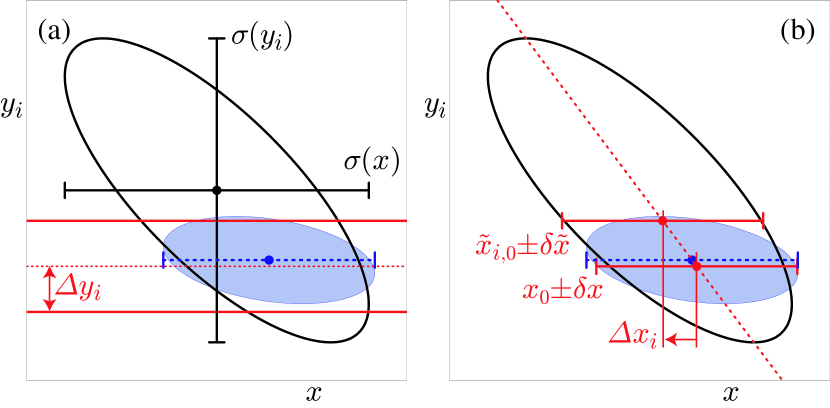
Figure 1: The left-hand plot, (a), compares the 68% confidence-level contours of a hypothetical measurement’s unconstrained (large ellipse) and constrained (filled ellipse) likelihoods, using the Gaussian constraint on $y_{i}$ represented by the horizontal band. The solid error bars represent the statistical uncertainties, $\sigma(x)$ and $\sigma(y_{i})$, of the unconstrained likelihood. The dashed error bar shows the statistical error on $x$ from a constrained simultaneous fit to $x$ and $y_{i}$. The right-hand plot, (b), illustrates the method described in the text of performing fits to $x$ only with $y_{i}$ fixed at different values. The dashed diagonal line between these fit results has the slope $\rho(x,y_{i})\sigma(y_{i})/\sigma(x)$ in the limit of a parabolic unconstrained likelihood. The result of the constrained simultaneous fit from (a) is shown as a dashed error bar on $x$.

In practice, the added technical complexity of a constrained fit with extra free parameters is not justified by the small increase in sensitivity, as long as the external constraints $\Delta y_{i}$ are sufficiently precise when compared with the sensitivities $\sigma(y_{i})$ to each $y_{i}$ of the data alone. Instead, the usual procedure adopted by the experiments is to perform a baseline fit with all $y_{i}$ fixed to nominal values $y_{i,0}$, obtaining $x=x_{0}\pm\delta x$. This baseline fit neglects the uncertainty due to $\Delta y_{i}$, but this error can be mostly recovered by repeating the fit separately for each external parameter $y_{i}$ with its value fixed at $y_{i}=y_{i,0}+\Delta y_{i}$ to obtain $x=\tilde{x}_{i,0}\pm\delta\tilde{x}$, as illustrated in Fig. 1(b). The absolute shift, $|\tilde{x}_{i,0}-x_{0}|$, in the central value of $x$ is what the experiments usually quote as their systematic uncertainty $\Delta x_{i}$ on $x$ due to the unknown value of $y_{i}$. Our procedure requires that we know not only the magnitude of this shift but also its sign. In the limit that the unconstrained data is represented by a parabolic likelihood, the signed shift is given by

$$\Delta x_{i}=\rho(x,y_{i})\frac{\sigma(x)}{\sigma(y_{i})}\,\Delta y_{i}\;,$$ (1)

where $\sigma(x)$ and $\rho(x,y_{i})$ are the statistical uncertainty on $x$ and the correlation between $x$ and $y_{i}$ in the unconstrained data. While our procedure is not equivalent to the constrained fit with extra parameters, it yields (in the limit of a parabolic unconstrained likelihood) a central value $x_{0}$ that agrees to ${\cal O}(\Delta y_{i}/\sigma(y_{i}))^{2}$ and an uncertainty $\delta x\oplus\Delta x_{i}$ that agrees to ${\cal O}(\Delta y_{i}/\sigma(y_{i}))^{4}$.

In order to combine two or more measurements that share systematics due to the same external parameters $y_{i}$, we would ideally perform a constrained simultaneous fit of all data samples to obtain values of $x$ and each $y_{i}$, being careful to only apply the constraint on each $y_{i}$ once. This is not practical since we generally do not have sufficient information to reconstruct the unconstrained likelihoods corresponding to each measurement. Instead, we perform the two-step approximate procedure described below.

Figs. 2(a,b) illustrate two statistically-independent measurements, $x_{1}\pm(\delta x_{1}\oplus\Delta x_{i,1})$ and $x_{2}\pm(\delta x_{i}\oplus\Delta x_{i,2})$, of the same hypothetical quantity $x$ (for simplicity, we only show the contribution of a single correlated systematic due to an external parameter $y_{i}$). As our knowledge of the external parameters $y_{i}$ evolves, it is natural that the different measurements of $x$ will assume different nominal values and ranges for each $y_{i}$. The first step of our procedure is to adjust the values of each measurement to reflect the current best knowledge of the values $y_{i}^{\prime}$ and ranges $\Delta y_{i}^{\prime}$ of the external parameters $y_{i}$, as illustrated in Figs. 2(c,b). We adjust the central values $x_{k}$ and correlated systematic uncertainties $\Delta x_{i,k}$ linearly for each measurement (indexed by $k$) and each external parameter (indexed by $i$):

$$x_{k}^{\prime} =x_{k}+\sum_{i}\,\frac{\Delta x_{i,k}}{\Delta y_{i,k}}\left(y_{i}^{\prime}-y_{i,k}\right)$$ (2)

$$\Delta x_{i,k}^{\prime} =\Delta x_{i,k}\cdot\frac{\Delta y_{i}^{\prime}}{\Delta y_{i,k}}\;.$$ (3)

This procedure is exact in the limit that the unconstrained likelihoods of each measurement is parabolic.

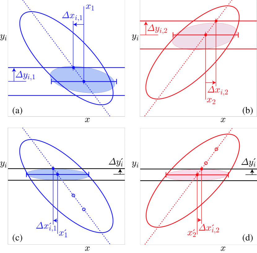
Figure 2: The upper plots, (a) and (b), show examples of two individual measurements to be combined. The large ellipses represent their unconstrained likelihoods, and the filled ellipses represent their constrained likelihoods. Horizontal bands indicate the different assumptions about the value and uncertainty of $y_{i}$ used by each measurement. The error bars show the results of the approximate method described in the text for obtaining $x$ by performing fits with $y_{i}$ fixed to different values. The lower plots, (c) and (d), illustrate the adjustments to accommodate updated and consistent knowledge of $y_{i}$ described in the text. Hollow circles mark the central values of the unadjusted fits to $x$ with $y$ fixed, which determine the dashed line used to obtain the adjusted values.

The second step of our procedure is to combine the adjusted measurements, $x_{k}^{\prime}\pm(\delta x_{k}\oplus\Delta x_{k,1}^{\prime}\oplus\Delta x_{k,2}^{\prime}\oplus\ldots)$ using the chi-square

$$\chi^{2}_{\text{comb}}(x,y_{1},y_{2},\ldots)\equiv\sum_{k}\,\frac{1}{\delta x_{k}^{2}}\left[x_{k}^{\prime}-\left(x+\sum_{i}\,(y_{i}-y_{i}^{\prime})\frac{\Delta x_{i,k}^{\prime}}{\Delta y_{i}^{\prime}}\right)\right]^{2}+\sum_{i}\,\left(\frac{y_{i}-y_{i}^{\prime}}{\Delta y_{i}^{\prime}}\right)^{2}\;,$$ (4)

and then minimize this $\chi^{2}$ to obtain the best values of $x$ and $y_{i}$ and their uncertainties, as illustrated in Fig. 3. Although this method determines new values for the $y_{i}$, we do not report them since the $\Delta x_{i,k}$ reported by each experiment are generally not intended for this purpose (for example, they may represent a conservative upper limit rather than a true reflection of a 68% confidence level).

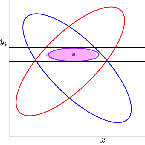
Figure 3: An illustration of the combination of two hypothetical measurements of $x$ using the method described in the text. The ellipses represent the unconstrained likelihoods of each measurement and the horizontal band represents the latest knowledge about $y_{i}$ that is used to adjust the individual measurements. The filled small ellipse shows the result of the exact method using ${\cal L}_{\text{comb}}$ and the hollow small ellipse and dot show the result of the approximate method using $\chi^{2}_{\text{comb}}$.

For comparison, the exact method we would perform if we had the unconstrained likelihoods ${\cal L}_{k}(x,y_{1},y_{2},\ldots)$ available for each measurement is to minimize the simultaneous constrained likelihood

$${\cal L}_{\text{comb}}(x,y_{1},y_{2},\ldots)\equiv\prod_{k}\,{\cal L}_{k}(x,y_{1},y_{2},\ldots)\,\prod_{i}\,{\cal L}_{i}(y_{i})\;,$$ (5)

with an independent Gaussian external constraint on each $y_{i}$

$${\cal L}_{i}(y_{i})\equiv\exp\left[-\frac{1}{2}\,\left(\frac{y_{i}-y_{i}^{\prime}}{\Delta y_{i}^{\prime}}\right)^{2}\right]\;.$$ (6)

The results of this exact method are illustrated by the filled ellipses in Figs. 3(a,b), and agree with our method in the limit that each ${\cal L}_{k}$ is parabolic and that each $\Delta y_{i}^{\prime}\ll\sigma(y_{i})$. In the case of a non-parabolic unconstrained likelihood, experiments would have to provide a description of ${\cal L}_{k}$ itself to allow an improved combination. In the case of some $\sigma(y_{i})\simeq\Delta y_{i}^{\prime}$, experiments are advised to perform a simultaneous measurement of both $x$ and $y$ so that their data will improve the world knowledge about $y$.

The algorithm described above is used as a default in the averages reported in the following sections. For some cases, somewhat simplified or more complex algorithms are used and noted in the corresponding sections.

Following the prescription described above, the central values and errors are rescaled to a common set of input parameters in the averaging procedures, according to the dependency on any of these input parameters. We try to use the most up-to-date values for these common inputs and the same values among the HFAG subgroups. For the parameters whose averages are produced by the HFAG, we use the updated values in the current update cycle. For other external parameters, we use the most recent PDG values.

The parameters and values used in this update cycle are listed in each subgroup section.

3 $b$-hadron production fractions, lifetimes and mixing parameters

Quantities such as $b$-hadron production fractions, $b$-hadron lifetimes, and neutral $B$-meson oscillation frequencies have been measured for many years at high-energy colliders, namely at LEP and SLC ($e^{+}e^{-}$ colliders at $\sqrt{s}=m_{Z}$) as well as at the first version of the Tevatron ($p\overline{p}$ collider at $\sqrt{s}=1.8~{}\rm TeV$). More recently, precise measurements of the $B^{0}$ and $B^{+}$ lifetimes, as well as of the $B^{0}$ oscillation frequency, have also been performed at the asymmetric $B$ factories, KEKB and PEPII ($e^{+}e^{-}$ colliders at $\sqrt{s}=m_{\mathchar 28935\relax(4S)}$). In most cases, these basic quantities, although interesting by themselves, can now be seen as necessary ingredients for the more complicated and refined analyses being currently performed at the asymmetric $B$ factories and at the upgraded Tevatron ($\sqrt{s}=1.96~{}\rm TeV$), in particular the time-dependent $C\!P$ asymmetry measurements. It is therefore important that the best experimental values of these quantities continue to be kept up-to-date and improved.

In several cases, the averages presented in this chapter are indeed needed and used as input for the results given in the subsequent chapters. However, within this chapter, some averages need the knowledge of other averages in a circular way. This “coupling”, which appears through the $b$-hadron fractions whenever inclusive or semi-exclusive measurements have to be considered, has been reduced significantly in the last years with increasingly precise exclusive measurements becoming available. To cope with this circularity, a rather involved averaging procedure had been developed, in the framework of the former LEP Heavy Flavour Steering Group. This is still in use now (details can be found in [2]), although simplifications can be envisaged in the future when even more precise exclusive measurements become available.

3.1 $b$-hadron production fractions

We consider here the relative fractions of the different $b$-hadron species found in an unbiased sample of weakly-decaying $b$ hadrons produced under some specific conditions. The knowledge of these fractions is useful to characterize the signal composition in inclusive $b$-hadron analyses, or to predict the background composition in exclusive analyses. Many analyses in $B$ physics need these fractions as input. We distinguish here the following two conditions: $\mathchar 28935\relax(4S)$ decays and high-energy collisions.

3.1.1 $b$-hadron production fractions in $\mathchar 28935\relax(4S)$ decays

Only pairs of the two lightest (charged and neutral) $B$ mesons can be produced in $\mathchar 28935\relax(4S)$ decays, and it is enough to determine the following branching fractions:

$$f^{+-} = \Gamma(\mathchar 28935\relax(4S)\to B^{+}B^{-})/\Gamma_{\rm tot}(\mathchar 28935\relax(4S))\,,$$ (7)

$$f^{00} = \Gamma(\mathchar 28935\relax(4S)\to B^{0}\overline{B}^{0})/\Gamma_{\rm tot}(\mathchar 28935\relax(4S))\,.$$ (8)

In practice, most analyses measure their ratio

$$R^{+-/00}=f^{+-}/f^{00}=\Gamma(\mathchar 28935\relax(4S)\to B^{+}B^{-})/\Gamma(\mathchar 28935\relax(4S)\to B^{0}\overline{B}^{0})\,,$$ (9)

which is easier to access experimentally. Since an inclusive (but separate) reconstruction of $B^{+}$ and $B^{0}$ is difficult, specific exclusive decay modes, ${B^{+}}\to x^{+}$ and ${B^{0}}\to x^{0}$, are usually considered to perform a measurement of $R^{+-/00}$, whenever they can be related by isospin symmetry (for example $B^{+}\to J/\psi K^{+}$ and $B^{0}\to J/\psi K^{0}$). Under the assumption that $\Gamma(B^{+}\to x^{+})=\Gamma(B^{0}\to x^{0})$, i.e. that isospin invariance holds in these $B$ decays, the ratio of the number of reconstructed $B^{+}\to x^{+}$ and $B^{0}\to x^{0}$ mesons is proportional to

$$\frac{f^{+-}\,{\cal B}(B^{+}\to x^{+})}{f^{00}\,{\cal B}(B^{0}\to x^{0})}=\frac{f^{+-}\,\Gamma({B^{+}}\to x^{+})\,\tau(B^{+})}{f^{00}\,\Gamma({B^{0}}\to x^{0})\,\tau(B^{0})}=\frac{f^{+-}}{f^{00}}\,\frac{\tau(B^{+})}{\tau(B^{0})}\,,$$ (10)

where $\tau(B^{+})$ and $\tau(B^{0})$ are the $B^{+}$ and $B^{0}$ lifetimes respectively. Hence the primary quantity measured in these analyses is $R^{+-/00}\,\tau(B^{+})/\tau(B^{0})$, and the extraction of $R^{+-/00}$ with this method therefore requires the knowledge of the $\tau(B^{+})/\tau(B^{0})$ lifetime ratio.

Table 1: Published measurements of the $B^{+}/B^{0}$ production ratio in $\mathchar 28935\relax(4S)$ decays, together with their average (see text). Systematic uncertainties due to the imperfect knowledge of $\tau(B^{+})/\tau(B^{0})$ are included.

Experiment	Ref.	Decay modes	Published value of	Assumed value
and year		or method	$R^{+-/00}=f^{+-}/f^{00}$	of $\tau(B^{+})/\tau(B^{0})$
CLEO, 2001	[5]	$J/\psi K^{(*)}$	$1.04\pm 0.07\pm 0.04$	$1.066\pm 0.024$
BABAR, 2002	[6]	$(c\overline{c})K^{(*)}$	$1.10\pm 0.06\pm 0.05$	$1.062\pm 0.029$
CLEO, 2002	[7]	$D^{*}\ell\nu$	$1.058\pm 0.084\pm 0.136$	$1.074\pm 0.028$
Belle, 2003	[8]	dilepton events	$1.01\pm 0.03\pm 0.09$	$1.083\pm 0.017$
BABAR, 2004	[9]	$J/\psi K$	$1.006\pm 0.036\pm 0.031$	$1.083\pm 0.017$
Average			$1.021\pm 0.034$ (tot)	$1.076\pm 0.008$

The published measurements of $R^{+-/00}$ are listed in Table 1 together with the corresponding assumed values of $\tau(B^{+})/\tau(B^{0})$. All measurements are based on the above-mentioned method, except the one from Belle, which is a by-product of the $B^{0}$ mixing frequency analysis using dilepton events (but note that it also assumes isospin invariance, namely $\Gamma(B^{+}\to\ell^{+}{\rm X})=\Gamma(B^{0}\to\ell^{+}{\rm X})$). The latter is therefore treated in a slightly different manner in the following procedure used to combine these measurements:

• each published value of $R^{+-/00}$ from CLEO and BABAR is first converted back to the original measurement of $R^{+-/00}\,\tau(B^{+})/\tau(B^{0})$, using the value of the lifetime ratio assumed in the corresponding analysis;

• a simple weighted average of these original measurements of $R^{+-/00}\,\tau(B^{+})/\tau(B^{0})$ from CLEO and BABAR (which do not depend on the assumed value of the lifetime ratio) is then computed, assuming no statistical or systematic correlations between them;

• the weighted average of $R^{+-/00}\,\tau(B^{+})/\tau(B^{0})$ is converted into a value of $R^{+-/00}$, using the latest average of the lifetime ratios, $\tau(B^{+})/\tau(B^{0})=1.076\pm 0.008$ (see Sec. 3.2.3);

• the Belle measurement of $R^{+-/00}$ is adjusted to the current values of $\tau(B^{0})=1.528\pm 0.009~{}\rm ps$ and $\tau(B^{+})/\tau(B^{0})=1.076\pm 0.008$ (see Sec. 3.2.3), using the quoted systematic uncertainties due to these parameters;

• the combined value of $R^{+-/00}$ from CLEO and BABAR is averaged with the adjusted value of $R^{+-/00}$ from Belle, assuming a 100% correlation of the systematic uncertainty due to the limited knowledge on $\tau(B^{+})/\tau(B^{0})$; no other correlation is considered.

The resulting global average,

$$R^{+-/00}=\frac{f^{+-}}{f^{00}}=1.021\pm 0.034\,,$$ (11)

is consistent with an equal production of charged and neutral $B$ mesons.

On the other hand, the BABAR collaboration has recently performed a direct measurement of the $f^{00}$ fraction using a novel method, which does not rely on isospin symmetry nor requires the knowledge of $\tau(B^{+})/\tau(B^{0})$. Its analysis, based on a comparison between the number of events where a single $B^{0}\to D^{*-}\ell^{+}\nu$ decay could be reconstructed and the number of events where two such decays could be reconstructed, yields [10]

$$f^{00}=0.487\pm 0.010\,\mbox{(stat)}\pm 0.008\,\mbox{(syst)}\,.$$ (12)

The two results of Eqs. (11) and (12) are of very different natures and completely independent of each other. Their product is equal to $f^{+-}=0.497\pm 0.021$, while another combination of them gives $f^{+-}+f^{00}=0.984\pm 0.031$, compatible with unity. Assuming $f^{+-}+f^{00}=1$, also consistent with CLEO’s observation that the fraction of $\mathchar 28935\relax(4S)$ decays to $B\kern 1.79993pt\overline{\kern-1.79993ptB}{}$ pairs is larger than 0.96 at 95% CL [11], the results of Eqs. (11) and (12) can be averaged (first converting Eq. (11) into a value of $f^{00}=1/(R^{+-/00}+1)$) to yield the following more precise estimates:

$$f^{00}=0.492\pm 0.007\,,~{}~{}~{}f^{+-}=1-f^{00}=0.508\pm 0.007\,,~{}~{}~{}\frac{f^{+-}}{f^{00}}=1.030\pm 0.029\,.$$ (13)

3.1.2 $b$-hadron production fractions at high energy

At high energy, all species of weakly-decaying $b$ hadrons can be produced, either directly or in strong and electromagnetic decays of excited $b$ hadrons. We assume here that the fractions of these different species are the same in unbiased samples of high-$p_{\rm T}$ $b$ jets originating from $Z^{0}$ decays or from $p\overline{p}$ collisions at the Tevatron. This hypothesis is plausible considering that, in both cases, the last step of the jet hadronization is a non-perturbative QCD process occurring at the scale of $\mathchar 28931\relax_{\rm QCD}$. On the other hand, there is no strong argument to claim that these fractions should be strictly equal, so this assumption should be checked experimentally. Although the available data is not sufficient at this time to perform a significant check, it is expected that the new data from Tevatron Run II may improve this situation and allow one to confirm or disprove this assumption with reasonable confidence. Meanwhile, the attitude adopted here is that these fractions are assumed to be equal at all high-energy colliders until demonstrated otherwise by experiment.

Contrary to what happens in the charm sector where the fractions of $D^{+}$ and $D^{0}$ are different, the relative amount of $B^{+}$ and $B^{0}$ is not affected by the electromagnetic decays of excited ${B^{+}}^{*}$ and ${B^{0}}^{*}$ states and strong decays of excited ${B^{+}}^{**}$ and ${B^{0}}^{**}$ states. Decays of the type ${B^{0}_{s}}^{**}\to B^{(*)}K$ also contribute to the $B^{+}$ and $B^{0}$ rates, but with the same magnitude if mass effects can be neglected. We therefore assume equal production of $B^{+}$ and $B^{0}$. We also neglect the production of weakly-decaying states made of several heavy quarks (like $B^{+}_{c}$ and other heavy baryons) which is known to be very small. Hence, for the purpose of determining the $b$-hadron fractions, we use the constraints

$$f_{u}=f_{d}~{}~{}~{}~{}\mbox{and}~{}~{}~{}f_{u}+f_{d}+f_{s}+f_{\rm baryon}=1\,,$$ (14)

where $f_{u}$, $f_{d}$, $f_{s}$ and $f_{\rm baryon}$ are the unbiased fractions of $B^{+}$, $B^{0}$, $B^{0}_{s}$ and $b$-baryons, respectively.

The LEP experiments have measured $f_{s}\times{\cal B}(B^{0}_{s}\to D_{s}^{-}\ell^{+}\nu_{\ell}\mbox{$X$})$ [12], ${\cal B}(b\to\mathchar 28931\relax_{b}^{0})\times{\cal B}(\mathchar 28931\relax_{b}^{0}\to\mathchar 28931\relax_{c}^{+}\ell^{-}\overline{\nu}_{\ell}\mbox{$X$})$ [13, 14] and ${\cal B}(b\to\mathchar 28932\relax_{b}^{-})\times{\cal B}(\mathchar 28932\relax_{b}^{-}\to\mathchar 28932\relax^{-}\ell^{-}\overline{\nu}_{\ell}\mbox{$X$})$ [15, 16] from partially reconstructed final states including a lepton, $f_{\rm baryon}$ from protons identified in $b$ events [17], and the production rate of charged $b$ hadrons [18]. The various $b$-hadron fractions have also been measured at CDF using electron-charm final states [19] and double semileptonic decays with $\phi\ell$ and $K^{*}\ell$ final states [20]. All these published results have been combined following the procedure and assumptions described in [2] to yield $f_{u}=f_{d}=0.403\pm 0.011$, $f_{s}=0.087\pm 0.021$ and $f_{\rm baryon}=0.107\pm 0.018$ under the constraints of Eq. (14). For this combination, other external inputs are used, e.g. the branching ratios of $B$ mesons to final states with a $D$, $D^{*}$ or $D^{**}$ in semileptonic decays, which are needed to evaluate the fraction of semileptonic $B^{0}_{s}$ decays with a $D_{s}^{-}$ in the final state.

Time-integrated mixing analyses performed with lepton pairs from $b\overline{b}$ events produced at high-energy colliders measure the quantity

$$\overline{\chi}=f^{\prime}_{d}\,\chi_{d}+f^{\prime}_{s}\,\chi_{s}\,,$$ (15)

where $f^{\prime}_{d}$ and $f^{\prime}_{s}$ are the fractions of $B^{0}$ and $B^{0}_{s}$ hadrons in a sample of semileptonic $b$-hadron decays, and where $\chi_{d}$ and $\chi_{s}$ are the $B^{0}$ and $B^{0}_{s}$ time-integrated mixing probabilities. Assuming that all $b$ hadrons have the same semileptonic decay width implies $f^{\prime}_{i}=f_{i}R_{i}$, where $R_{i}=\tau_{i}/\tau_{b}$ is the ratio of the lifetime $\tau_{i}$ of species $i$ to the average $b$-hadron lifetime $\tau_{b}=\sum_{i}f_{i}\tau_{i}$. Hence measurements of the mixing probabilities $\overline{\chi}$, $\chi_{d}$ and $\chi_{s}$ can be used to improve our knowledge of $f_{u}$, $f_{d}$, $f_{s}$ and $f_{\rm baryon}$. In practice, the above relations yield another determination of $f_{s}$ obtained from $f_{\rm baryon}$ and mixing information,

$$f_{s}=\frac{1}{R_{s}}\frac{(1+r)\overline{\chi}-(1-f_{\rm baryon}R_{\rm baryon})\chi_{d}}{(1+r)\chi_{s}-\chi_{d}}\,,$$ (16)

where $r=R_{u}/R_{d}=\tau(B^{+})/\tau(B^{0})$.

The published measurements of $\overline{\chi}$ performed by the LEP experiments have been combined by the LEP Electroweak Working Group to yield $\overline{\chi}=0.1257\pm 0.0042$ [21]. This can be compared with a recent measurement from CDF, $\overline{\chi}=0.152\pm 0.013$ [22], obtained from an analysis of the Run I data. The two estimates deviate from each other by $1.9\,\sigma$, and could be an indication that the production fractions of $b$ hadrons at the $Z$ peak or at the Tevatron are not the same. Although this discrepancy is not very significant it should be carefully monitored in the future. We choose to combine these two results in a simple weighted average, assuming no correlations, and, following the PDG prescription, we multiply the combined uncertainty by $1.9$ to account for the discrepancy. Our world average is then

$$\overline{\chi}=0.1281\pm 0.0076\,.$$ (17)

Table 2: Fractions of the different $b$-hadron species in an unbiased sample of weakly-decaying $b$ hadrons produced at high energy, obtained from both direct and mixing measurements.

$b$-hadron	Fraction	Correlation coefficients
species		with $f_{d}=f_{u}$	and $f_{s}$
$B^{0}$, $B^{+}$	$f_{d}=f_{u}=0.399\pm 0.010$
$B^{0}_{s}$	$f_{s}=0.102\pm 0.014$	$-0.564$
$b$ baryons	$f_{\rm baryon}=0.100\pm 0.017$	$-0.724$	$-0.162$

Introducing the latter result in Eq. (16), together with our world average $\chi_{d}=0.189\pm 0.002$ (see Eq. (43) of Sec. 3.3.1), the assumption $\chi_{s}=1/2$ (justified by the large value of $\Delta m_{s}$, see Eq. (48) in Sec. 3.3.2), the best knowledge of the lifetimes (see Sec. 3.2) and the estimate of $f_{\rm baryon}$ given above, yields $f_{s}=0.116\pm 0.021$, an estimate dominated by the mixing information. Taking into account all known correlations (including the one introduced by $f_{\rm baryon}$), this result is then combined with the set of fractions obtained from direct measurements (given above), to yield the improved estimates of Table 2, still under the constraints of Eq. (14). As can be seen, our knowledge on the mixing parameters substantially reduces the uncertainty on $f_{s}$, despite the rather strong deweighting introduced in the computation of the world average of $\overline{\chi}$. It should be noted that the results are correlated, as indicated in Table 2.

3.2 $b$-hadron lifetimes

In the spectator model the decay of $b$-flavored hadrons $H_{b}$ is governed entirely by the flavor changing $b\to Wq$ transition ($q=c,u$). For this very reason, lifetimes of all $b$-flavored hadrons are the same in the spectator approximation regardless of the (spectator) quark content of the $H_{b}$. In the early 1990’s experiments became sophisticated enough to start seeing the differences of the lifetimes among various $H_{b}$ species. The first theoretical calculations of the spectator quark effects on $H_{b}$ lifetime emerged only few years earlier.

Currently, most of such calculations are performed in the framework of the Heavy Quark Expansion, HQE. In the HQE, under certain assumptions (most important of which is that of quark-hadron duality), the decay rate of an $H_{b}$ to an inclusive final state $f$ is expressed as the sum of a series of expectation values of operators of increasing dimension, multiplied by the correspondingly higher powers of $\mathchar 28931\relax_{\rm QCD}/m_{b}$:

$$\Gamma_{H_{b}\to f}=|CKM|^{2}\sum_{n}c_{n}^{(f)}\Bigl{(}\frac{\mathchar 28931\relax_{\rm QCD}}{m_{b}}\Bigr{)}^{n}\langle H_{b}|O_{n}|H_{b}\rangle,$$ (18)

where $|CKM|^{2}$ is the relevant combination of the CKM matrix elements. Coefficients $c_{n}^{(f)}$ of this expansion, known as Operator Product Expansion [23], can be calculated perturbatively. Hence, the HQE predicts $\Gamma_{H_{b}\to f}$ in the form of an expansion in both $\mathchar 28931\relax_{\rm QCD}/m_{b}$ and $\alpha_{s}(m_{b})$. The precision of current experiments makes it mandatory to go to the next-to-leading order in QCD, i.e. to include correction of the order of $\alpha_{s}(m_{b})$ to the $c_{n}^{(f)}$’s. All non-perturbative physics is shifted into the expectation values $\langle H_{b}|O_{n}|H_{b}\rangle$ of operators $O_{n}$. These can be calculated using lattice QCD or QCD sum rules, or can be related to other observables via the HQE [24]. One may reasonably expect that powers of $\mathchar 28931\relax_{\rm QCD}/m_{b}$ provide enough suppression that only the first few terms of the sum in Eq. (18) matter.

Theoretical predictions are usually made for the ratios of the lifetimes (with $\tau(B^{0})$ chosen as the common denominator) rather than for the individual lifetimes, for this allows several uncertainties to cancel. The precision of the current HQE calculations (see Refs. [25, 26, 27] for the latest updates) is in some instances already surpassed by the measurements, e.g. in the case of $\tau(B^{+})/\tau(B^{0})$. Also, HQE calculations are not assumption-free. More accurate predictions are a matter of progress in the evaluation of the non-perturbative hadronic matrix elements and verifying the assumptions that the calculations are based upon. However, the HQE, even in its present shape, draws a number of important conclusions, which are in agreement with experimental observations:

• The heavier the mass of the heavy quark the smaller is the variation in the lifetimes among different hadrons containing this quark, which is to say that as $m_{b}\to\infty$ we retrieve the spectator picture in which the lifetimes of all $H_{b}$’s are the same. This is well illustrated by the fact that lifetimes in the $b$ sector are all very similar, while in the $c$ sector ($m_{c}<m_{b}$) lifetimes differ by as much as a factor of 2.

• The non-perturbative corrections arise only at the order of $\mathchar 28931\relax_{\rm QCD}^{2}/m_{b}^{2}$, which translates into differences among $H_{b}$ lifetimes of only a few percent.

• It is only the difference between meson and baryon lifetimes that appears at the $\mathchar 28931\relax_{\rm QCD}^{2}/m_{b}^{2}$ level. The splitting of the meson lifetimes occurs at the $\mathchar 28931\relax_{\rm QCD}^{3}/m_{b}^{3}$ level, yet it is enhanced by a phase space factor $16\pi^{2}$ with respect to the leading free $b$ decay.

To ensure that certain sources of systematic uncertainty cancel, lifetime analyses are sometimes designed to measure a ratio of lifetimes. However, because of the differences in decay topologies, abundance (or lack thereof) of decays of a certain kind, etc., measurements of the individual lifetimes are more common. In the following section we review the most common types of the lifetime measurements. This discussion is followed by the presentation of the averaging of the various lifetime measurements, each with a brief description of its particularities.

3.2.1 Lifetime measurements, uncertainties and correlations

In most cases lifetime of an $H_{b}$ is estimated from a flight distance and a $\beta\gamma$ factor which is used to convert the geometrical distance into the proper decay time. Methods of accessing lifetime information can roughly be divided in the following five categories:

1. Inclusive (flavor blind) measurements. These measurements are aimed at extracting the lifetime from a mixture of $b$-hadron decays, without distinguishing the decaying species. Often the knowledge of the mixture composition is limited, which makes these measurements experiment-specific. Also, these measurements have to rely on Monte Carlo for estimating the $\beta\gamma$ factor, because the decaying hadrons are not fully reconstructed. On the bright side, these usually are the largest statistics $b$-hadron lifetime measurements that are accessible to a given experiment, and can, therefore, serve as an important performance benchmark.

2. Measurements in semileptonic decays of a specific $H_{b}$. $W$ from $b\to Wc$ produces $\ell\nu_{l}$ pair ($\ell=e,\mu$) in about 21% of the cases. Electron or muon from such decays is usually a well-detected signature, which provides for clean and efficient trigger. $c$ quark from $b\to Wc$ transition and the other quark(s) making up the decaying $H_{b}$ combine into a charm hadron, which is reconstructed in one or more exclusive decay channels. Knowing what this charmed hadron is allows one to separate, at least statistically, different $H_{b}$ species. The advantage of these measurements is in statistics, which usually is superior to that of the exclusively reconstructed $H_{b}$ decays. Some of the main disadvantages are related to the difficulty of estimating lepton+charm sample composition and Monte Carlo reliance for the $\beta\gamma$ factor estimate.

3. Measurements in exclusively reconstructed decays. These have the advantage of complete reconstruction of decaying $H_{b}$, which allows one to infer the decaying species as well as to perform precise measurement of the $\beta\gamma$ factor. Both lead to generally smaller systematic uncertainties than in the above two categories. The downsides are smaller branching ratios, larger combinatoric backgrounds, especially in $H_{b}\rightarrow H_{c}\pi(\pi\pi)$ and multi-body $H_{c}$ decays, or in a hadron collider environment with non-trivial underlying event. $H_{b}\to J/\psi H_{s}$ are relatively clean and easy to trigger on $J/\psi\to\ell^{+}\ell^{-}$, but their branching fraction is only about 1%.

4. Measurements at asymmetric B factories. In the $\mathchar 28935\relax(4S)\rightarrow B\overline{B}$ decay, the $B$ mesons ($B^{+}$ or $B^{0}$) are essentially at rest in the $\mathchar 28935\relax(4S)$ rest frame. This makes lifetime measurements impossible with experiments, such as CLEO, in which $\mathchar 28935\relax(4S)$ produced at rest. At asymmetric $B$ factories $\mathchar 28935\relax(4S)$ is boosted resulting in $B$ and $\overline{B}$ moving nearly parallel to each other. The lifetime is inferred from the distance $\Delta z$ separating $B$ and $\overline{B}$ decay vertices and $\mathchar 28935\relax(4S)$ boost known from colliding beam energies. In order to maximize the precision of the measurement, one $B$ meson is reconstructed in the $D^{(*)}\ell\nu_{\ell}$ decay. The other $B$ is typically not fully reconstructed, only position of its decay vertex is determined. These measurements benefit from very large statistics, but suffer from poor $\Delta z$ resolution.

5. Direct measurement of lifetime ratios. This method has so far been only applied in the measurement of $\tau(B^{+})/\tau(B^{0})$. The ratio of the lifetimes is extracted from the dependence of the observed relative number of $B^{+}$ and $B^{0}$ candidates (both reconstructed in semileptonic decays) on the proper decay time.

In some of the latest analyses, measurements of two (e.g. $\tau(B^{+})$ and $\tau(B^{+})/\tau(B^{0})$) or three (e.g. $\tau(B^{+})$, $\tau(B^{+})/\tau(B^{0})$, and $\Delta m_{d}$) quantities are combined. This introduces correlations among measurements. Another source of correlations among the measurements are the systematic effects, which could be common to an experiment or to an analysis technique across the experiments. When calculating the averages, such correlations are taken into account per general procedure, described in Ref. [28].

3.2.2 Inclusive $b$-hadron lifetimes

The inclusive $b$ hadron lifetime is defined as $\tau_{b}=\sum_{i}f_{i}\tau_{i}$ where $\tau_{i}$ are the individual species lifetimes and $f_{i}$ are the fractions of the various species present in an unbiased sample of weakly-decaying $b$ hadrons produced at a high-energy collider. This quantity is certainly less fundamental than the lifetimes of the individual species, the latter being much more useful in comparisons of the measurements with the theoretical predictions. Nonetheless, we perform the averaging of the inclusive lifetime measurements for completeness as well as for the reason that they might be of interest as “technical numbers.”

Table 3: Measurements of average $b$-hadron lifetimes.

Experiment	Method	Data set	$\tau_{b}$ (ps)	Ref.
ALEPH	Dipole	91	$1.511\pm 0.022\pm 0.078$	[29]
DELPHI	All track i.p. (2D)	91–92	$1.542\pm 0.021\pm 0.045$	[30]a
DELPHI	Sec. vtx	91–93	$1.582\pm 0.011\pm 0.027$	[31]a
DELPHI	Sec. vtx	94–95	$1.570\pm 0.005\pm 0.008$	[32]
L3	Sec. vtx + i.p.	91–94	$1.556\pm 0.010\pm 0.017$	[33]b
OPAL	Sec. vtx	91–94	$1.611\pm 0.010\pm 0.027$	[34]
SLD	Sec. vtx	93	$1.564\pm 0.030\pm 0.036$	[35]
Average set 1 ($b$ vertex)			$1.572\pm 0.009$
ALEPH	Lepton i.p. (3D)	91–93	$1.533\pm 0.013\pm 0.022$	[36]
L3	Lepton i.p. (2D)	91–94	$1.544\pm 0.016\pm 0.021$	[33]b
OPAL	Lepton i.p. (2D)	90–91	$1.523\pm 0.034\pm 0.038$	[37]
Average set 2 ($b\to\ell$)			$1.537\pm 0.020$
CDF	$J/\psi$ vtx	92–95	$1.533\pm 0.015^{+0.035}_{-0.031}$	[38]
Average of all above			$1.568\pm 0.009$
a The combined DELPHI result quoted in [31] is 1.575 $\pm$ 0.010 $\pm$ 0.026 ps.
b The combined L3 result quoted in [33] is 1.549 $\pm$ 0.009 $\pm$ 0.015 ps.

In practice, an unbiased measurement of the inclusive lifetime is difficult to achieve, because it would imply an efficiency which is guaranteed to be the same across species. So most of the measurements are biased. In an attempt to group analyses which are expected to select the same mixture of $b$ hadrons, the available results (given in Table 3) are divided into the following three sets:

1. measurements at LEP and SLD that accept any $b$-hadron decay, based on topological reconstruction (secondary vertex or track impact parameters);

2. measurements at LEP based on the identification of a lepton from a $b$ decay; and

3. measurements at the Tevatron based on inclusive $H_{b}\to J/\psi X$ reconstruction, where the $J/\psi$ is fully reconstructed.

The measurements of the first set are generally considered as estimates of $\tau_{b}$, although the efficiency to reconstruct a secondary vertex most probably depends, in an analysis-specific way, on the number of tracks coming from the vertex, thereby depending on the type of the $H_{b}$. Even though these efficiency variations can in principle be accounted for using Monte Carlo simulations (which inevitably contain assumptions on branching fractions), the $H_{b}$ mixture in that case can remain somewhat ill-defined and could be slightly different among analyses in this set.

On the contrary, the mixtures corresponding to the other two sets of measurements are better defined in the limit where the reconstruction and selection efficiency of a lepton or a $J/\psi$ from an $H_{b}$ does not depend on the decaying hadron type. These mixtures are given by the production fractions and the inclusive branching fractions for each $H_{b}$ species to give a lepton or a $J/\psi$. In particular, under the assumption that all $b$ hadrons have the same semileptonic decay width, the analyses of the second set should measure $\tau(b\to\ell)=(\sum_{i}f_{i}\tau_{i}^{2})/(\sum_{i}f_{i}\tau_{i})$ which is necessarily larger than $\tau_{b}$ if lifetime differences exist. Given the present knowledge on $\tau_{i}$ and $f_{i}$, $\tau(b\to\ell)-\tau_{b}$ is expected to be of the order of 0.01 $\rm ps$.

Measurements by SLC and LEP experiments are subject to a number of common systematic uncertainties, such as those due to (lack of knowledge of) $b$ and $c$ fragmentation, $b$ and $c$ decay models, ${\cal B}(B\to\ell)$, ${\cal B}(B\to c\to\ell)$, ${\cal B}(c\to\ell)$, $\tau_{c}$, and $H_{b}$ decay multiplicity. In the averaging, these systematic uncertainties are assumed to be 100% correlated. The averages for the sets defined above (also given in Table 3) are

$$\tau(b~{}\mbox{vertex}) = 1.572\pm 0.009~{}\rm ps\,,$$ (19)

$$\tau(b\to\ell) = 1.537\pm 0.020~{}\rm ps\,,$$ (20)

$$\tau(b\to J/\psi) = 1.533^{+0.038}_{-0.034}~{}\rm ps\,,$$ (21)

whereas an average of all measurements, ignoring mixture differences, yields $1.568\pm 0.009~{}\rm ps$.

3.2.3 $B^{0}$ and $B^{+}$ lifetimes and their ratio

Table 4: Measurements of the $B^{0}$ lifetime.

Experiment	Method	Data set	$\tau(B^{0})$ (ps)	Ref.
ALEPH	$D^{(*)}\ell$	91–95	$1.518\pm 0.053\pm 0.034$	[39]
ALEPH	Exclusive	91–94	$1.25^{+0.15}_{-0.13}\pm 0.05$	[40]
ALEPH	Partial rec. $\pi^{+}\pi^{-}$	91–94	$1.49^{+0.17+0.08}_{-0.15-0.06}$	[40]
DELPHI	$D^{(*)}\ell$	91–93	$1.61^{+0.14}_{-0.13}\pm 0.08$	[41]
DELPHI	Charge sec. vtx	91–93	$1.63\pm 0.14\pm 0.13$	[42]
DELPHI	Inclusive $D^{*}\ell$	91–93	$1.532\pm 0.041\pm 0.040$	[43]
DELPHI	Charge sec. vtx	94–95	$1.531\pm 0.021\pm 0.031$	[32]
L3	Charge sec. vtx	94–95	$1.52\pm 0.06\pm 0.04$	[44]
OPAL	$D^{(*)}\ell$	91–93	$1.53\pm 0.12\pm 0.08$	[45]
OPAL	Charge sec. vtx	93–95	$1.523\pm 0.057\pm 0.053$	[46]
OPAL	Inclusive $D^{*}\ell$	91–00	$1.541\pm 0.028\pm 0.023$	[47]
SLD	Charge sec. vtx $\ell$	93–95	$1.56^{+0.14}_{-0.13}\pm 0.10$	[48]a
SLD	Charge sec. vtx	93–95	$1.66\pm 0.08\pm 0.08$	[48]a
CDF	$D^{(*)}\ell$	92–95	$1.474\pm 0.039^{+0.052}_{-0.051}$	[49]
CDF	Excl. $J/\psi K^{*0}$	92–95	$1.497\pm 0.073\pm 0.032$	[50]
CDF	Excl. $J/\psi K^{*0}$	02–04	$1.539\pm 0.051\pm 0.008$	[51]p
CDF	Incl. $D^{(*)}\ell$	02–04	$1.473\pm 0.036\pm 0.054$	[52]p
CDF	Excl. $D^{-}(3)\pi$	02–04	$1.511\pm 0.023\pm 0.013$	[53]p
DØ	Excl. $J/\psi K^{*0}$	02–04	$1.473^{+0.052}_{-0.050}\pm 0.023$	[54]
DØ	Excl. $J/\psi K_{S}$	02–04	$1.400^{+0.110}_{-0.100}\pm 0.030$	[55]
BABAR	Exclusive	99–00	$1.546\pm 0.032\pm 0.022$	[56]
BABAR	Inclusive $D^{*}\ell$	99–01	$1.529\pm 0.012\pm 0.029$	[57]
BABAR	Exclusive $D^{*}\ell$	99–02	$1.523^{+0.024}_{-0.023}\pm 0.022$	[58]
BABAR	Incl. $D^{*}\pi$, $D^{*}\rho$	99–01	$1.533\pm 0.034\pm 0.038$	[59]
BABAR	Inclusive $D^{*}\ell$	99–04	$1.501\pm 0.008\pm 0.030$	[60]p
Belle	Exclusive	00–03	$1.534\pm 0.008\pm 0.010$	[61]
Average			$1.528\pm 0.009$
a The combined SLD result quoted in [48] is 1.64 $\pm$ 0.08 $\pm$ 0.08 ps.
p Preliminary.

After a number of years of dominating these averages LEP experiments culminated with the recent publication [32] by DELPHI collaboration and yielded the scene to the asymmetric $B$ factories and the Tevatron experiments. The $B$ factories have been very successful in utilizing their potential – in only a few years of running, BABAR and, to a greater extent, Belle, have struck a balance between the statistical and the systematic uncertainties, with both being close to (or even better than) the impressive 1%. In the meanwhile, CDF and DØ have emerged as significant contributors to the field as the Tevatron Run II data flowed in. Both appear to enjoy relatively small systematic effects, and while current statistical uncertainties of their measurements are factors of 2 to 4 larger than those of their $B$-factory counterparts, both Tevatron experiments stand to increase their samples by an order of magnitude.

Table 5: Measurements of the $B^{+}$ lifetime.

Experiment	Method	Data set	$\tau(B^{+})$ (ps)	Ref.
ALEPH	$D^{(*)}\ell$	91–95	$1.648\pm 0.049\pm 0.035$	[39]
ALEPH	Exclusive	91–94	$1.58^{+0.21+0.04}_{-0.18-0.03}$	[40]
DELPHI	$D^{(*)}\ell$	91–93	$1.61\pm 0.16\pm 0.12$	[41]a
DELPHI	Charge sec. vtx	91–93	$1.72\pm 0.08\pm 0.06$	[42]a
DELPHI	Charge sec. vtx	94–95	$1.624\pm 0.014\pm 0.018$	[32]
L3	Charge sec. vtx	94–95	$1.66\pm 0.06\pm 0.03$	[44]
OPAL	$D^{(*)}\ell$	91–93	$1.52\pm 0.14\pm 0.09$	[45]
OPAL	Charge sec. vtx	93–95	$1.643\pm 0.037\pm 0.025$	[46]
SLD	Charge sec. vtx $\ell$	93–95	$1.61^{+0.13}_{-0.12}\pm 0.07$	[48]b
SLD	Charge sec. vtx	93–95	$1.67\pm 0.07\pm 0.06$	[48]b
CDF	$D^{(*)}\ell$	92–95	$1.637\pm 0.058^{+0.045}_{-0.043}$	[49]
CDF	Excl. $J/\psi K$	92–95	$1.636\pm 0.058\pm 0.025$	[50]
CDF	Excl. $J/\psi K$	02–04	$1.662\pm 0.033\pm 0.008$	[51]p
CDF	Incl. $D^{0}\ell$	02–04	$1.653\pm 0.029^{+0.033}_{-0.031}$	[52]p
CDF	Excl. $D^{0}\pi$	02–04	$1.661\pm 0.027\pm 0.013$	[53]p
BABAR	Exclusive	99–00	$1.673\pm 0.032\pm 0.023$	[56]
Belle	Exclusive	00–03	$1.635\pm 0.011\pm 0.011$	[61]
Average			$1.643\pm 0.010$
a The combined DELPHI result quoted in [42] is $1.70\pm 0.09$ ps.
b The combined SLD result quoted in [48] is $1.66\pm 0.06\pm 0.05$ ps.
p Preliminary.

At present time we are in an interesting position of having three sets of measurements (from LEP/SLC, $B$ factories and the Tevatron) that originate from different environments, obtained using substantially different techniques and are precise enough for incisive comparison.

Table 6: Measurements of the ratio $\tau(B^{+})/\tau(B^{0})$.

Experiment	Method	Data set	Ratio $\tau(B^{+})/\tau(B^{0})$	Ref.
ALEPH	$D^{(*)}\ell$	91–95	$1.085\pm 0.059\pm 0.018$	[39]
ALEPH	Exclusive	91–94	$1.27^{+0.23+0.03}_{-0.19-0.02}$	[40]
DELPHI	$D^{(*)}\ell$	91–93	$1.00^{+0.17}_{-0.15}\pm 0.10$	[41]
DELPHI	Charge sec. vtx	91–93	$1.06^{+0.13}_{-0.11}\pm 0.10$	[42]
DELPHI	Charge sec. vtx	94–95	$1.060\pm 0.021\pm 0.024$	[32]
L3	Charge sec. vtx	94–95	$1.09\pm 0.07\pm 0.03$	[44]
OPAL	$D^{(*)}\ell$	91–93	$0.99\pm 0.14^{+0.05}_{-0.04}$	[45]
OPAL	Charge sec. vtx	93–95	$1.079\pm 0.064\pm 0.041$	[46]
SLD	Charge sec. vtx $\ell$	93–95	$1.03^{+0.16}_{-0.14}\pm 0.09$	[48]a
SLD	Charge sec. vtx	93–95	$1.01^{+0.09}_{-0.08}\pm 0.05$	[48]a
CDF	$D^{(*)}\ell$	92–95	$1.110\pm 0.056^{+0.033}_{-0.030}$	[49]
CDF	Excl. $J/\psi K$	92–95	$1.093\pm 0.066\pm 0.028$	[50]
CDF	Excl. $J/\psi K$	02–04	$1.080\pm 0.042$	[51]p
CDF	Incl. $D\ell$	02–04	$1.123\pm 0.040^{+0.041}_{-0.039}$	[52]p
CDF	Excl. $D\pi$	02–04	$1.10\pm 0.02\pm 0.01$	[53]p
DØ	$D^{*+}\mu$ $D^{0}\mu$ ratio	02–04	$1.080\pm 0.016\pm 0.014$	[62]p
BABAR	Exclusive	99–00	$1.082\pm 0.026\pm 0.012$	[56]
Belle	Exclusive	00–03	$1.066\pm 0.008\pm 0.008$	[61]
Average			$1.076\pm 0.008$
a The combined SLD result quoted in [48] is $1.01\pm 0.07\pm 0.06$.
p Preliminary.

The averaging of $\tau(B^{+})$, $\tau(B^{0})$ and $\tau(B^{+})/\tau(B^{0})$ measurements is summarized in Tables 4, 5, and 6. For $\tau(B^{+})/\tau(B^{0})$ we averaged only the measurements of this quantity provided by experiments rather than using all available knowledge, which would have included, for example, $\tau(B^{+})$ and $\tau(B^{0})$ measurements which did not contribute to any of the ratio measurements.

The following sources of correlated (within experiment/machine) systematic uncertainties have been considered:

• for SLC/LEP measurements – $D^{**}$ branching ratio uncertainties [2], momentum estimation of $b$ mesons from $Z^{0}$ decays ($b$-quark fragmentation parameter $\langle X_{E}\rangle=0.702\pm 0.008$ [2]), $B^{0}_{s}$ and $b$ baryon lifetimes (see Secs. 3.2.4 and 3.2.6), and $b$ hadron fractions at high energy (see Table 2).

• for BABAR measurements – alignment, $z$ scale, PEP-II boost, sample composition (where applicable)

• for DØ and CDF Run II measurements – alignment (separately within each experiment)

The resultant averages are:

$$\tau(B^{0}) = 1.528\pm 0.009~{}\rm ps\,,$$ (22)

$$\tau(B^{+}) = 1.643\pm 0.010~{}\rm ps\,,$$ (23)

$$\tau(B^{+})/\tau(B^{0}) = 1.076\pm 0.008\,.$$ (24)

3.2.4 $B^{0}_{s}$ lifetime

Similar to the kaon system, neutral $B$ mesons contain short- and long-lived components, since the light (L) and heavy (H) eigenstates, $B_{\rm L}$ and $B_{\rm H}$, differ not only in their masses, but also in their widths with $\Delta\Gamma=\Gamma_{\rm L}-\Gamma_{\rm H}$. In the case of the $B^{0}_{s}$ system, $\Delta\Gamma_{s}$ can be particularly large. The current theoretical prediction in the Standard Model for the fractional width difference is $\Delta\Gamma_{s}/\Gamma_{s}=0.12\pm 0.05$ [63], where $\Gamma_{s}=(\Gamma_{\rm L}+\Gamma_{\rm H})/2$. Specific measurements of $\Delta\Gamma_{s}$ and $\Gamma_{s}$ are explained in Sec. 3.3.2, but the result for $\Gamma_{s}$ is quoted here.

Neglecting $C\!P$ violation, which is expected to be small in the $B^{0}_{s}$ system [63], the $B^{0}_{s}$ mass eigenstates are also $C\!P$ eigenstates. In the Standard Model assuming no $C\!P$ violation in the $B^{0}_{s}$ system, $\Gamma_{\rm L}$ is the width of the $C\!P$-even state and $\Gamma_{\rm H}$ the width of the $C\!P$-odd state. Final states can be decomposed into $C\!P$-even and $C\!P$-odd components, each with a different lifetime.

In view of a possibly substantial width difference, and the fact that various decay channels will have different proportions of the $B_{\rm L}$ and $B_{\rm H}$ eigenstates, the straight average of all available $B^{0}_{s}$ lifetime measurements is rather ill-defined. Therefore, the $B^{0}_{s}$ lifetime measurements are broken down into three categories and averaged separately.

• Flavor-specific decays, such as semileptonic $B_{s}\to D_{s}\ell\nu$ or $B_{s}\to D_{s}\pi$, will have equal fractions of $B_{\rm L}$ and $B_{\rm H}$ at time zero, where $\tau_{\rm L}=1/\Gamma_{\rm L}$ is expected to be the shorter-lived component and $\tau_{\rm H}=1/\Gamma_{\rm H}$ expected to be the longer-lived component. A superposition of two exponentials thus results with decay widths $\Gamma_{s}\pm\Delta\Gamma_{s}/2$. Fitting to a single exponential results in a measure of a flavor-specific lifetime, one obtains [64]:

  $$\tau(B^{0}_{s})_{\rm fs}=\frac{1}{\Gamma_{s}}\frac{{1+\left(\frac{\Delta\Gamma_{s}}{2\Gamma_{s}}\right)^{2}}}{{1-\left(\frac{\Delta\Gamma_{s}}{2\Gamma_{s}}\right)^{2}}}.$$ (25)

  As given in Table 7, the flavor-specific $B^{0}_{s}$ lifetime world average is:

  $$\tau(B^{0}_{s})_{\rm fs}=1.472\pm 0.045~{}\rm ps\,.$$ (26)

  This world average will be used later in Sec. 3.3.2 in combination with other measurements to find $\overline{\tau}(B^{0}_{s})=1/\Gamma_{s}$ and $\Delta\Gamma_{s}$.

  The following correlated systematic errors were considered: average $B$ lifetime used in backgrounds, $B^{0}_{s}$ decay multiplicity, and branching ratios used to determine backgrounds (e.g. ${\cal B}(B\to D_{s}D)$). A knowledge of the multiplicity of $B^{0}_{s}$ decays is important for measurements that partially reconstruct the final state such as $B\to D_{s}\mbox{$X$}$ (where $X$ is not a lepton). The boost deduced from Monte Carlo simulation depends on the multiplicity used. Since this is not well known, the multiplicity in the simulation is varied and this range of values observed is taken to be a systematic. Similarly not all the branching ratios for the potential background processes are measured. Where they are available, the PDG values are used for the error estimate. Where no measurements are available estimates can usually be made by using measured branching ratios of related processes and using some reasonable extrapolation.

Table 7: Measurements of the $B^{0}_{s}$ lifetime.

Experiment	Method	Data set	$\tau(B^{0}_{s})$ (ps)	Ref.
ALEPH	$D_{s}\ell$	91–95	$1.54^{+0.14}_{-0.13}\pm 0.04$	[65]
CDF	$D_{s}\ell$	92–96	$1.36\pm 0.09^{+0.06}_{-0.05}$	[66]
DELPHI	$D_{s}\ell$	91–95	$1.42^{+0.14}_{-0.13}\pm 0.03$	[67]
OPAL	$D_{s}\ell$	90–95	$1.50^{+0.16}_{-0.15}\pm 0.04$	[68]
DØ	$D_{s}\mu$	02–04	$1.420\pm 0.043\pm 0.057$	[69]p
CDF	$D_{s}\pi,D_{s}\pi\pi\pi$	02–04	$1.60\pm 0.10\pm 0.02$	[70]p
Average of flavor-specific measurements			$1.472\pm 0.045$
ALEPH	$D_{s}h$	91–95	$1.47\pm 0.14\pm 0.08$	[71]
DELPHI	$D_{s}h$	91–95	$1.53^{+0.16}_{-0.15}\pm 0.07$	[72]
OPAL	$D_{s}$ incl.	90–95	$1.72^{+0.20+0.18}_{-0.19-0.17}$	[73]
Average of all above $D_{s}$ measurements			$1.479\pm 0.044$
CDF	$J/\psi\phi$	92–95	$1.34^{+0.23}_{-0.19}\pm 0.05$	[38]
CDF	$J/\psi\phi$	02–04	$1.369\pm 0.100^{+0.008}_{-0.010}$	[51]p
DØ	$J/\psi\phi$	02–04	$1.444^{+0.098}_{-0.090}\pm 0.02$	[54]
Average of $J/\psi\phi$ measurements			$1.404\pm 0.066$
p Preliminary.

• $B^{0}_{s}\to D^{+}_{s}X$ decays. Included in Table 7 are measurements of lifetimes using samples of $B^{0}_{s}$ decays to $D_{s}$ plus hadrons, and hence into a less known mixture of $C\!P$-states. A lifetime weighted this way can still be a useful input for analyses examining such an inclusive sample. These are separated in Table 7 and combined with the semileptonic lifetime to obtain:

  $$\tau(B^{0}_{s})_{D_{s}{\rm X}}=1.479\pm 0.044~{}\rm ps\,.$$ (27)

• Fully exclusive $B^{0}_{s}$ $\to J/\psi\phi$ decays are expected to be dominated by the $C\!P$-even state and its lifetime. First measurements of the $C\!P$ mix for this decay mode are outlined in Sec. 3.3.2. CDF and DØ measurements from this particular mode $B^{0}_{s}\to J/\psi\phi$ are combined into an average given in Table 7. There are no correlations between the measurements for this fully exclusive channel, and the world average for this specific decay is:

  $$\tau(B^{0}_{s})_{J/\psi\phi}=1.404\pm 0.066~{}\rm ps\,.$$ (28)

  A caveat is that different experimental acceptances will likely lead to different admixtures of the $C\!P$-even and $C\!P$-odd states, and fits to a single exponential may result in inherently different measurements of these quantities.

Finally, as will be shown in Sec. 3.3.2, measurements of $\Delta\Gamma_{s}$, including separation into $C\!P$-even and $C\!P$-odd components, give

$$\overline{\tau}(B^{0}_{s})=1/\Gamma_{s}=1.42^{+0.06}_{-0.07}~{}\rm ps\,,$$ (29)

and when combined with the flavor-specific lifetime measurements:

$$\overline{\tau}(B^{0}_{s})=1/\Gamma_{s}=1.405^{+0.043}_{-0.047}~{}\rm ps\,.$$ (30)

3.2.5 $B^{+}_{c}$ lifetime

There are currently two measurements of the lifetime of the $B^{+}_{c}$ meson from CDF [74] and DØ [75] using the semileptonic decay mode $B^{+}_{c}\to J/\psi\ell$ and fitting simultaneously to the mass and lifetime using the vertex formed with the leptons from the decay of the $J/\psi$ and the third lepton. Correction factors to estimate the boost due to the missing neutrino are used. Mass values of $6.40\pm 0.39\pm 0.13$ GeV/$c^{2}$ and $5.95^{+0.14}_{-0.13}\pm 0.34$ GeV/$c^{2}$, respectively, are found by fitting to the tri-lepton invariant mass spectrum. These mass measurements are consistent to within uncertainties. Correlated systematic errors include the impact of the uncertainty of the $B^{+}_{c}$ $p_{T}$ spectrum on the correction factors, the level of feed-down from $\psi(2S)$, MC modeling of the decay model varying from phase space to the ISGW model, and mass variations. Values of the $B^{+}_{c}$ lifetime are given in Table 8 and the world average is determined to be:

$$\tau(B^{+}_{c})=0.45\pm 0.12~{}\rm ps\,.$$ (31)

Table 8: Measurements of the $B^{+}_{c}$ lifetime.

Experiment	Method	Data set	$\tau(B^{+}_{c})$ (ps)	Ref.
CDF	$J/\psi\ell$	92–95	$0.46^{+0.18}_{-0.16}\pm 0.03$	[74]
DØ	$J/\psi\mu$	02–04	$0.448^{+0.123}_{-0.096}\pm 0.121$	[75]p
Average			$0.45\pm 0.12$
p Preliminary.

3.2.6 $\mathchar 28931\relax_{b}^{0}$ and $b$-baryon lifetimes

The most precise measurements of the $b$-baryon lifetime originate from two classes of partially reconstructed decays. In the first class, decays with an exclusively reconstructed $\mathchar 28931\relax_{c}^{+}$ baryon and a lepton of opposite charge are used. These products are more likely to occur in the decay of $\mathchar 28931\relax_{b}^{0}$ baryons. In the second class, more inclusive final states with a baryon ($p$, $\overline{p}$, $\mathchar 28931\relax$, or $\overline{\mathchar 28931\relax}$) and a lepton have been used, and these final states can generally arise from any $b$ baryon.

The following sources of correlated systematic uncertainties have been considered: experimental time resolution within a given experiment, $b$-quark fragmentation distribution into weakly decaying $b$ baryons, $\mathchar 28931\relax_{b}^{0}$ polarization, decay model, and evaluation of the $b$-baryon purity in the selected event samples. In computing the averages the central values of the masses are scaled to $M(\mathchar 28931\relax_{b}^{0})=5624\pm 9~{}\rm MeV/\mbox{$c$}^{2}$ [76] and $M(\mbox{$b$-baryon})=5670\pm 100~{}\rm MeV/\mbox{$c$}^{2}$.

The meaning of decay model and the correlations are not always clear. Uncertainties related to the decay model are dominated by assumptions on the fraction of $n$-body decays. To be conservative it is assumed that it is correlated whenever given as an error. DELPHI varies the fraction of 4-body decays from 0.0 to 0.3. In computing the average, the DELPHI result is corrected for $0.2\pm 0.2$.

Furthermore, in computing the average, the semileptonic decay results are corrected for a polarization of $-0.45^{+0.19}_{-0.17}$ [2] and a $\mathchar 28931\relax_{b}^{0}$ fragmentation parameter $\langle X_{E}\rangle=0.70\pm 0.03$ [77].

Inputs to the averages are given in Table 9. The world average lifetime of $b$ baryons is then:

$$\langle\tau(\mbox{$b$-baryon})\rangle=1.210\pm 0.048~{}\rm ps\,.$$ (32)

Keeping only $\mathchar 28931\relax^{\pm}_{c}\ell^{\mp}$ and $\mathchar 28931\relax\ell^{-}\ell^{+}$ final states, as representative of the $\mathchar 28931\relax_{b}^{0}$ baryon, the following lifetime is obtained:

$$\tau(\mathchar 28931\relax_{b}^{0})=1.232\pm 0.072~{}\rm ps\,.$$ (33)

Averaging the measurements based on the $\mathchar 28932\relax^{\mp}\ell^{\mp}$ final states [16, 15] gives a lifetime value for a sample of events containing $\mathchar 28932\relax_{b}^{0}$ and $\mathchar 28932\relax_{b}^{-}$ baryons:

$$\langle\tau(\mathchar 28932\relax_{b})\rangle=1.39^{+0.34}_{-0.28}~{}\rm ps\,.$$ (34)

Table 9: Measurements of the $b$-baryon lifetimes.

Experiment	Method	Data set	Lifetime (ps)	Ref.
ALEPH	$\mathchar 28931\relax_{c}^{+}\ell$	91–95	$1.18^{+0.13}_{-0.12}\pm 0.03$	[14]
ALEPH	$\mathchar 28931\relax\ell^{-}\ell^{+}$	91–95	$1.30^{+0.26}_{-0.21}\pm 0.04$	[14]
CDF	$\mathchar 28931\relax_{c}^{+}\ell$	91–95	$1.32\pm 0.15\pm 0.06$	[78]
CDF	$J/\psi\mathchar 28931\relax$	02–03	$1.25\pm 0.26\pm 0.10$	[79]p
DØ	$J/\psi\mathchar 28931\relax$	02–04	$1.22^{+0.22}_{-0.18}\pm 0.04$	[55]
DELPHI	$\mathchar 28931\relax_{c}^{+}\ell$	91–94	$1.11^{+0.19}_{-0.18}\pm 0.05$	[80]a
OPAL	$\mathchar 28931\relax_{c}^{+}\ell$, $\mathchar 28931\relax\ell^{-}\ell^{+}$	90–95	$1.29^{+0.24}_{-0.22}\pm 0.06$	[68]
Average of above 7 ($\mathchar 28931\relax_{b}^{0}$ lifetime)			$1.232\pm 0.072$
ALEPH	$\mathchar 28931\relax\ell$	91–95	$1.20^{+0.08}_{-0.08}\pm 0.06$	[14]
DELPHI	$\mathchar 28931\relax\ell\pi$ vtx	91–94	$1.16\pm 0.20\pm 0.08$	[80]a
DELPHI	$\mathchar 28931\relax\mu$ i.p.	91–94	$1.10^{+0.19}_{-0.17}\pm 0.09$	[81]a
DELPHI	$p\ell$	91–94	$1.19\pm 0.14\pm 0.07$	[80]a
OPAL	$\mathchar 28931\relax\ell$ i.p.	90–94	$1.21^{+0.15}_{-0.13}\pm 0.10$	[82]b
OPAL	$\mathchar 28931\relax\ell$ vtx	90–94	$1.15\pm 0.12\pm 0.06$	[82]b
Average of above 13 ($b$-baryon lifetime)			$1.210\pm 0.048$
ALEPH	$\mathchar 28932\relax\ell$	90–95	$1.35^{+0.37+0.15}_{-0.28-0.17}$	[16]
DELPHI	$\mathchar 28932\relax\ell$	91–93	$1.5^{+0.7}_{-0.4}\pm 0.3$	[15]
Average of above 2 ($\mathchar 28932\relax_{b}$ lifetime)			$1.39^{+0.34}_{-0.28}$
a The combined DELPHI result quoted in [80] is $1.14\pm 0.08\pm 0.04$ ps.
b The combined OPAL result quoted in [82] is $1.16\pm 0.11\pm 0.06$ ps.
p Preliminary.

3.2.7 Summary and comparison with theoretical predictions

Averages of lifetimes of specific $b$ hadron species are collected in Table 11.

Table 10: Summary of lifetimes of different $b$ hadron species.

$b$ hadron species	Measured lifetime
$B^{+}$	$1.643\pm 0.010~{}\rm ps$
$B^{0}$	$1.528\pm 0.009~{}\rm ps$
$B^{0}_{s}$ ($\to$ flavor specific)	$1.472\pm 0.045~{}\rm ps$
$B^{0}_{s}$ ($\to J/\psi\phi$)	$1.404\pm 0.066~{}\rm ps$
$B^{0}_{s}$ ($1/\Gamma_{s}$)	$1.405^{+0.043}_{-0.047}~{}\rm ps$
$B^{+}_{c}$	$0.45\pm 0.12~{}\rm ps$
$\mathchar 28931\relax_{b}^{0}$	$1.232\pm 0.072~{}\rm ps$
$\mathchar 28932\relax_{b}$ mixture	$1.39^{+0.34}_{-0.28}~{}\rm ps$
$b$-baryon mixture	$1.210\pm 0.048~{}\rm ps$
$b$-hadron mixture	$1.568\pm 0.009~{}\rm ps$

Table 11: Ratios of $b$-hadron lifetimes relative to the $B^{0}$ lifetime and theoretical ranges predicted by theory [27].

Lifetime ratio	Measured value	Predicted range
$\tau(B^{+})/\tau(B^{0})$	$1.076\pm 0.008$	1.04 – 1.08
$\overline{\tau}(B^{0}_{s})/\tau(B^{0})^{a}$	$0.920\pm 0.030$	0.99 – 1.01
$\tau(\mathchar 28931\relax_{b}^{0})/\tau(B^{0})$	$0.806\pm 0.047$	0.81 – 0.91
$\tau(\mbox{$b$-baryon})/\tau(B^{0})$	$0.792\pm 0.032$	0.81 – 0.91
a Using $\overline{\tau}(B^{0}_{s})=1/\Gamma_{s}=2/(\Gamma_{\rm L}+\Gamma_{\rm H})$.

As described in Sec. 3.2, Heavy Quark Effective Theory can be employed to explain the hierarchy of $\tau(B^{+}_{c})\ll\tau(\mathchar 28931\relax_{b}^{0})<\tau(B^{0}_{s})\approx\tau(B^{0})<\tau(B^{+})$, and used to predict the ratios between lifetimes. Typical predictions are compared to the measured lifetime ratios in Table 11.

A recent prediction of the ratio between the $B^{+}$ and $B^{0}$ lifetimes, is $1.06\pm 0.02$ [26], in good agreement with experiment.

The total widths of the $B^{0}_{s}$ and $B^{0}$ mesons are expected to be very close and differ by at most 1% [83, 27]. However, the experimental ratio $\overline{\tau}(B^{0}_{s})/\tau(B^{0})$, where $\overline{\tau}(B^{0}_{s})=1/\Gamma_{s}$ is obtained from $\Delta\Gamma_{s}$ and flavour-specific lifetime measurements, now appears to be smaller than 1, at deviation with respect to the prediction. At present this discrepancy is not very significant.

The ratio $\tau(\mathchar 28931\relax_{b}^{0})/\tau(B^{0})$ has particularly been the source of theoretical scrutiny since earlier calculations [84] predicted a value greater than 0.90, almost two sigma higher than the world average at the time. Recent calculations of this ratio that include higher order effects predict a ratio between the $\mathchar 28931\relax_{b}^{0}$ and $B^{0}$ lifetimes of $0.86\pm 0.05$ [27] and reduces this difference. Ref. [27] presents probability density functions of its predictions with variation of theoretical inputs, and the indicated errors (and ranges in Table 11) are the RMS of the distributions.

3.3 Neutral $B$-meson mixing

There are two neutral $B-\overline{B}$ systems, $B^{0}-\overline{B}^{0}$ and $B^{0}_{s}-\overline{B}^{0}_{s}$, which both exhibit the phenomenon of particle-antiparticle mixing. For each of these systems, there are two mass eigenstates which are linear combinations of the two flavour states, $B$ or $\overline{B}$. We consider the case where a neutral $B$ meson is produced and detected in a flavour state, through its decay to a flavour-specific final state. There are four different time-dependent probabilities; if $C\!PT$ is conserved (which will be assumed throughout), they can be written as

$$\left\{\begin{array}[]{rcl}{\cal P}(B\to B)&=&\frac{e^{-\Gamma t}}{2}\left[\cosh\!\left(\frac{\Delta\Gamma}{2}t\right)+\cos\!\left(\Delta mt\right)\right]\\ {\cal P}(B\to\overline{B})&=&\frac{e^{-\Gamma t}}{2}\left[\cosh\!\left(\frac{\Delta\Gamma}{2}t\right)-\cos\!\left(\Delta mt\right)\right]\left|\frac{q}{p}\right|^{2}\\ {\cal P}(\overline{B}\to B)&=&\frac{e^{-\Gamma t}}{2}\left[\cosh\!\left(\frac{\Delta\Gamma}{2}t\right)-\cos\!\left(\Delta mt\right)\right]\left|\frac{p}{q}\right|^{2}\\ {\cal P}(\overline{B}\to\overline{B})&=&\frac{e^{-\Gamma t}}{2}\left[\cosh\!\left(\frac{\Delta\Gamma}{2}t\right)+\cos\!\left(\Delta mt\right)\right]\end{array}\right.\,,$$ (35)

where $t$ is the proper time of the system (i.e. the time interval between the production and the decay in the rest frame of the $B$ meson) and $\Gamma=1/\tau(B)$ is the average decay width. At the $B$ factories, only the proper-time difference $\Delta t$ between the decays of the two neutral $B$ mesons from the $\mathchar 28935\relax(4S)$ can be determined, but, because the two $B$ mesons evolve coherently (keeping opposite flavours as long as none of them has decayed), the above formulae remain valid if $t$ is replaced with $\Delta t$ and the production flavour is replaced by the flavour at the time of the decay of the accompanying $B$ meson in a flavour specific state. As can be seen in the above expressions, the mixing probabilities depend on the following three observables: the mass difference $\Delta m$ and the decay width difference $\Delta\Gamma$ between the two mass eigenstates, and the parameter $|q/p|^{2}$ which signals $C\!P$ violation in the mixing if $|q/p|^{2}\neq 1$.

In the following sections we review in turn the experimental knowledge on these three parameters, separately for the $B^{0}$ meson ($\Delta m_{d}$, $\Delta\Gamma_{d}$, $|q/p|_{d}$) and the $B^{0}_{s}$ meson ($\Delta m_{s}$, $\Delta\Gamma_{s}$, $|q/p|_{s}$).

3.3.1 $B^{0}$ mixing parameters

$C\!P$ violation parameter $|q/p|_{d}$

Evidence for $C\!P$ violation in $B^{0}$ mixing has been searched for, both with flavor-specific and inclusive $B^{0}$ decays, in samples where the initial flavor state is tagged. In the case of semileptonic (or other flavor-specific) decays, where the final state tag is also available, the following asymmetry

$${\cal A}_{\rm SL}=\frac{N(\hbox{$\overline{B}^{0}$}(t)\to\ell^{+}\nu_{\ell}X)-N(\hbox{$B^{0}$}(t)\to\ell^{-}\overline{\nu}_{\ell}X)}{N(\hbox{$\overline{B}^{0}$}(t)\to\ell^{+}\nu_{\ell}X)+N(\hbox{$B^{0}$}(t)\to\ell^{-}\overline{\nu}_{\ell}X)}=\frac{|p/q|_{d}^{2}-|q/p|_{d}^{2}}{|p/q|_{d}^{2}+|q/p|_{d}^{2}}$$ (36)

has been measured, either in time-integrated analyses at CLEO [85, 86, 87] and CDF [88], or in time-dependent analyses at OPAL [89], ALEPH [90], BABAR [91, 92] and Belle [93]. In the inclusive case, also investigated and published at ALEPH [90] and OPAL [94], no final state tag is used, and the asymmetry [95]

$$\frac{N(\hbox{$B^{0}$}(t)\to{\rm all})-N(\hbox{$\overline{B}^{0}$}(t)\to{\rm all})}{N(\hbox{$B^{0}$}(t)\to{\rm all})+N(\hbox{$\overline{B}^{0}$}(t)\to{\rm all})}\simeq{\cal A}_{\rm SL}\left[\frac{\Delta m_{d}}{2\Gamma_{d}}\sin(\Delta m_{d}\,t)-\sin^{2}\left(\frac{\Delta m_{d}\,t}{2}\right)\right]$$ (37)

must be measured as a function of the proper time to extract information on $C\!P$ violation. In all cases asymmetries compatible with zero have been found, with a precision limited by the available statistics. A simple average of all published results for the $B^{0}$ meson [86, 87, 89, 90, 91, 92, 94] and of the preliminary Belle result [93] yields

$${\cal A}_{\rm SL}=-0.0026\pm 0.0067$$ (38)

or, equivalently through Eq. (36),

$$|q/p|_{d}=1.0013\pm 0.0034\,.$$ (39)

This result, summarized in Table 12, is compatible with no $C\!P$ violation in the mixing, an assumption we make for the rest of this section.

Table 12: Measurements of $C\!P$ violation in $B^{0}$ mixing and their average in terms of both ${\cal A}_{\rm SL}$ and $|q/p|_{d}$. The individual results are listed as quoted in the original publications, or converted to an ${\cal A}_{\rm SL}$ value. When two errors are quoted, the first one is statistical and the second one systematic.

Exp. & Ref.	Method	Measured ${\cal A}_{\rm SL}$			Measured $|q/p|_{d}$
CLEO [86]	partial hadronic rec.	$+0.017$ $\,\pm$	0.070 $\pm$	0.014
CLEO [87]	dileptons	$+0.013$ $\,\pm$	0.050 $\pm$	0.005
CLEO [87]	average of above two	$+0.014$ $\,\pm$	0.041 $\pm$	0.006
OPAL [89]	leptons	$+0.008$ $\,\pm$	0.028 $\pm$	0.012
OPAL [94]	inclusive (Eq. (37))	$+0.005$ $\,\pm$	0.055 $\pm$	0.013
ALEPH [90]	leptons	$-0.037$ $\,\pm$	0.032 $\pm$	0.007
ALEPH [90]	inclusive (Eq. (37))	$+0.016$ $\,\pm$	0.034 $\pm$	0.009
ALEPH [90]	average of above two	$-0.013$ $\,\pm$	0.026 (tot)
BABAR [92]	dileptons	$+0.005$ $\,\pm$	0.012 $\pm$	0.014	0.998 $\,\pm$	0.006 $\pm$	0.007
BABAR [91]	full hadronic rec.				$1.029$ $\,\pm$	0.013 $\pm$	0.011
Belle [93]	dileptons (prel.)	$-0.0013$ $\,\pm$	0.0060 $\pm$	0.0056	1.0006 $\,\pm$	0.0030 $\pm$	0.0028
	Average of all above	$-0.0026\pm 0.0067$ (tot)			$1.0013\pm 0.0034$  (tot)

Mass and decay width differences $\Delta m_{d}$ and $\Delta\Gamma_{d}$

Table 13: Time-dependent measurements included in the $\Delta m_{d}$ average. The results obtained from multi-dimensional fits involving also the $B^{0}$ (and $B^{+}$) lifetimes as free parameter(s) [58, 60, 61] have been converted into one-dimensional measurements of $\Delta m_{d}$. All the measurements have then been adjusted to a common set of physics parameters before being combined. The latest BABAR result [60] as well as the CDF2 and D0 results are preliminary.

Experiment	Method		$\Delta m_{d}$ in $\rm ps^{-1}$			$\Delta m_{d}$ in $\rm ps^{-1}$
and Ref.	rec.	tag	before adjustment			after adjustment
ALEPH [96]	$\ell$	$Q_{\rm jet}$	$0.404$	$\pm 0.045$	$\pm 0.027$
ALEPH [96]	$\ell$	$\ell$	$0.452$	$\pm 0.039$	$\pm 0.044$
ALEPH [96]	above two combined		$0.422$	$\pm 0.032$	$\pm 0.026$	$0.440$	$\pm 0.032$	${}^{+0.021}_{-0.020}$
ALEPH [96]	$D^{*}$	$\ell,Q_{\rm jet}$	$0.482$	$\pm 0.044$	$\pm 0.024$	$0.482$	$\pm 0.044$	$\pm 0.024$
DELPHI [97]	$\ell$	$Q_{\rm jet}$	$0.493$	$\pm 0.042$	$\pm 0.027$	$0.505$	$\pm 0.042$	$\pm 0.024$
DELPHI [97]	$\pi^{*}\ell$	$Q_{\rm jet}$	$0.499$	$\pm 0.053$	$\pm 0.015$	$0.501$	$\pm 0.053$	$\pm 0.015$
DELPHI [97]	$\ell$	$\ell$	$0.480$	$\pm 0.040$	$\pm 0.051$	$0.491$	$\pm 0.040$	${}^{+0.049}_{-0.048}$
DELPHI [97]	$D^{*}$	$Q_{\rm jet}$	$0.523$	$\pm 0.072$	$\pm 0.043$	$0.518$	$\pm 0.072$	$\pm 0.043$
DELPHI [98]	vtx	comb	$0.531$	$\pm 0.025$	$\pm 0.007$	$0.530$	$\pm 0.025$	$\pm 0.006$
L3 [99]	$\ell$	$\ell$	$0.458$	$\pm 0.046$	$\pm 0.032$	$0.472$	$\pm 0.046$	$\pm 0.029$
L3 [99]	$\ell$	$Q_{\rm jet}$	$0.427$	$\pm 0.044$	$\pm 0.044$	$0.435$	$\pm 0.044$	$\pm 0.042$
L3 [99]	$\ell$	$\ell\mbox{(IP)}$	$0.462$	$\pm 0.063$	$\pm 0.053$	$0.485$	$\pm 0.063$	$\pm 0.047$
OPAL [100]	$\ell$	$\ell$	$0.430$	$\pm 0.043$	${}^{+0.028}_{-0.030}$	$0.461$	$\pm 0.043$	${}^{+0.018}_{-0.017}$
OPAL [101]	$\ell$	$Q_{\rm jet}$	$0.444$	$\pm 0.029$	${}^{+0.020}_{-0.017}$	$0.466$	$\pm 0.029$	${}^{+0.015}_{-0.014}$
OPAL [102]	$D^{*}\ell$	$Q_{\rm jet}$	$0.539$	$\pm 0.060$	$\pm 0.024$	$0.544$	$\pm 0.060$	$\pm 0.023$
OPAL [102]	$D^{*}$	$\ell$	$0.567$	$\pm 0.089$	${}^{+0.029}_{-0.023}$	$0.571$	$\pm 0.089$	${}^{+0.028}_{-0.022}$
OPAL [103]	$\pi^{*}\ell$	$Q_{\rm jet}$	$0.497$	$\pm 0.024$	$\pm 0.025$	$0.496$	$\pm 0.024$	$\pm 0.025$
CDF1 [104]	$D\ell$	SST	$0.471$	${}^{+0.078}_{-0.068}$	${}^{+0.033}_{-0.034}$	$0.470$	${}^{+0.078}_{-0.068}$	${}^{+0.033}_{-0.034}$
CDF1 [105]	$\mu$	$\mu$	$0.503$	$\pm 0.064$	$\pm 0.071$	$0.512$	$\pm 0.064$	$\pm 0.070$
CDF1 [106]	$\ell$	$\ell,Q_{\rm jet}$	$0.500$	$\pm 0.052$	$\pm 0.043$	$0.534$	$\pm 0.052$	$\pm 0.036$
CDF1 [107]	$D^{*}\ell$	$\ell$	$0.516$	$\pm 0.099$	${}^{+0.029}_{-0.035}$	$0.523$	$\pm 0.099$	${}^{+0.028}_{-0.035}$
CDF2 [108]	$D^{(*)}\ell$	OST	$0.497$	$\pm 0.028$	$\pm 0.015$	$0.497$	$\pm 0.028$	$\pm 0.015$
CDF2 [109]	$B^{0}$	SST	$0.526$	$\pm 0.056$	$\pm 0.005$	$0.526$	$\pm 0.056$	$\pm 0.005$
DØ [110]	$D^{*}\mu$	comb	$0.456$	$\pm 0.034$	$\pm 0.025$	$0.456$	$\pm 0.034$	$\pm 0.025$
BABAR [111]	$B^{0}$	$\ell,K,\mbox{NN}$	$0.516$	$\pm 0.016$	$\pm 0.010$	$0.520$	$\pm 0.016$	$\pm 0.008$
BABAR [112]	$\ell$	$\ell$	$0.493$	$\pm 0.012$	$\pm 0.009$	$0.489$	$\pm 0.012$	$\pm 0.006$
BABAR [60]	$D^{*}\ell\nu\mbox{(part)}$	$\ell$	$0.523$	$\pm 0.004$	$\pm 0.007$	$0.521$	$\pm 0.004$	$\pm 0.007$
BABAR [58]	$D^{*}\ell\nu$	$\ell,K,\mbox{NN}$	$0.492$	$\pm 0.018$	$\pm 0.014$	$0.491$	$\pm 0.018$	$\pm 0.013$
Belle [113]	$D^{*}\pi\mbox{(part)}$	$\ell$	$0.509$	$\pm 0.017$	$\pm 0.020$	$0.512$	$\pm 0.017$	$\pm 0.019$
Belle [8]	$\ell$	$\ell$	$0.503$	$\pm 0.008$	$\pm 0.010$	$0.506$	$\pm 0.008$	$\pm 0.009$
Belle [61]	$B^{0},D^{*}\ell\nu$	comb	$0.511$	$\pm 0.005$	$\pm 0.006$	$0.512$	$\pm 0.005$	$\pm 0.007$
World average (all above measurements included):						$0.510$	$\pm 0.003$	$\pm 0.004$

– ALEPH, DELPHI, L3, OPAL and CDF1 only:    $0.495$ $\pm 0.010$ $\pm 0.009$       – Above measurements of BABAR and Belle only:    $0.511$ $\pm 0.003$ $\pm 0.005$

Many time-dependent $B^{0}$–$\overline{B}^{0}$ oscillation analyses have been performed by the ALEPH, BABAR, Belle, CDF, DØ, DELPHI, L3 and OPAL collaborations. The corresponding measurements of $\Delta m_{d}$ are summarized in Table 3.3.1, where only the most recent results are listed (i.e. measurements superseded by more recent ones have been omitted). Although a variety of different techniques have been used, the individual $\Delta m_{d}$ results obtained at high-energy colliders have remarkably similar precision. Their average is compatible with the recent and more precise measurements from the asymmetric $B$ factories. The systematic uncertainties are not negligible; they are often dominated by sample composition, mistag probability, or $b$-hadron lifetime contributions. Before being combined, the measurements are adjusted on the basis of a common set of input values, including the averages of the $b$-hadron fractions and lifetimes given in this report (see Secs. 3.1 and 3.2). Some measurements are statistically correlated. Systematic correlations arise both from common physics sources (fractions, lifetimes, branching ratios of $b$ hadrons), and from purely experimental or algorithmic effects (efficiency, resolution, flavour tagging, background description). Combining all published measurements listed in Table 3.3.1 and accounting for all identified correlations as described in [2] yields $\Delta m_{d}=0.510\pm 0.003\pm 0.004~{}\rm ps^{-1}$.

On the other hand, ARGUS and CLEO have published measurements of the time-integrated mixing probability $\chi_{d}$ [114, 85, 86], which average to $\chi_{d}=0.182\pm 0.015$. Following Ref. [86], the width difference $\Delta\Gamma_{d}$ could in principle be extracted from the measured value of $\Gamma_{d}=1/\tau(B^{0})$ and the above averages for $\Delta m_{d}$ and $\chi_{d}$ (provided that $\Delta\Gamma_{d}$ has a negligible impact on the $\Delta m_{d}$ analyses that have assumed $\Delta\Gamma_{d}=0$), using the relation

$$\chi_{d}=\frac{x_{d}^{2}+y_{d}^{2}}{2(x_{d}^{2}+1)}~{}~{}~{}\mbox{with}~{}~{}x_{d}=\frac{\Delta m_{d}}{\Gamma_{d}}~{}~{}~{}\mbox{and}~{}~{}y_{d}=\frac{\Delta\Gamma_{d}}{2\Gamma_{d}}\,.$$ (40)

However, direct time-dependent studies provide much stronger constraints: DELPHI published the result $|\Delta\Gamma_{d}|/\Gamma_{d}<18\%$ at 95% CL [98], while BABAR recently obtained $-8.4\%<{\rm sign}({\rm Re}\lambda_{C\!P})\Delta\Gamma_{d}/\Gamma_{d}<6.8\%$ at 90% CL [91], where $\lambda_{C\!P}=(q/p)_{d}(\overline{A}_{C\!P}/A_{C\!P})$ is defined for a $C\!P$-even final state and where $\Delta\Gamma_{d}$ is defined as $\Delta\Gamma_{d}=\Gamma(B^{0}_{\rm H})-\Gamma(B^{0}_{\rm L})$ (the sensitivity to the overall sign of ${\rm sign}({\rm Re}\lambda_{C\!P})\Delta\Gamma_{d}/\Gamma_{d}$ comes from the use of $B^{0}$ decays to $C\!P$ final states). Combining these two results after adjustment to $1/\Gamma_{d}=\tau(B^{0})=1.528\pm 0.009~{}\rm ps$ yields

$${\rm sign}({\rm Re}\lambda_{C\!P})\Delta\Gamma_{d}/\Gamma_{d}=-0.009\pm 0.037\,.$$ (41)

The sign of ${\rm Re}\lambda_{C\!P}$ is not measured, but expected to be positive from the global fits of the Unitarity Triangle within the Standard Model.

Assuming $\Delta\Gamma_{d}=0$ and using $1/\Gamma_{d}=\tau(B^{0})=1.528\pm 0.009~{}\rm ps$, the $\Delta m_{d}$ and $\chi_{d}$ results are combined through Eq. (40) to yield the world average

$$\Delta m_{d}=0.509\pm 0.004~{}\rm ps^{-1}\,,$$ (42)

or, equivalently,

$$x_{d}=0.778\pm 0.008~{}~{}~{}\mbox{and}~{}~{}~{}\chi_{d}=0.189\pm 0.002\,.$$ (43)

Figure 4 compares the $\Delta m_{d}$ values obtained by the different experiments.

Figure 4: The $B^{0}$–$\overline{B}^{0}$ oscillation frequency $\Delta m_{d}$ as measured by the different experiments. The averages quoted for ALEPH, L3 and OPAL are taken from the original publications, while the ones for DELPHI, CDF, BABAR, and Belle have been computed from the individual results listed in Table 3.3.1 without performing any adjustments. The time-integrated measurements of $\chi_{d}$ from the symmetric $B$ factory experiments ARGUS and CLEO have been converted to a $\Delta m_{d}$ value using $\tau(B^{0})=1.528\pm 0.009~{}\rm ps$. The two global averages have been obtained after adjustments of all the individual $\Delta m_{d}$ results of Table 3.3.1 (see text).

The $B^{0}$ mixing averages given in Eqs. (42) and (43) and the $b$-hadron fractions of Table 2 have been obtained in a fully consistent way, taking into account the fact that the fractions are computed using the $\chi_{d}$ value of Eq. (43) and that many individual measurements of $\Delta m_{d}$ at high energy depend on the assumed values for the $b$-hadron fractions. Furthermore, this set of averages is consistent with the lifetime averages of Sec. 3.2.

It should be noted that the most recent (and precise) analyses at the asymmetric $B$ factories measure $\Delta m_{d}$ as a result of a multi-dimensional fit. The preliminary BABAR analysis [60], based on partially reconstructed $B^{0}\to D^{*}\ell\nu$ decays, extracts simultaneously $\Delta m_{d}$ and $\tau(B^{0})$ in a way similar to the published BABAR analysis based on fully reconstructed $B^{0}\to D^{*}\ell\nu$ decays [58], while the latest Belle published analysis [61], based on fully reconstructed hadronic $B^{0}$ decays and $B^{0}\to D^{*}\ell\nu$ decays, extracts simultaneously $\Delta m_{d}$, $\tau(B^{0})$ and $\tau(B^{+})$. The measurements of $\Delta m_{d}$ and $\tau(B^{0})$ of these three analyses are displayed in Table 14 and in Fig. 5. Their two-dimensional average, taking into account all statistical and systematic correlations, and expressed at $\tau(B^{+})=1.643\pm 0.010~{}\rm ps$, is

$$\left.\begin{array}[]{r@{}l}\Delta m_{d}=0.514\pm 0.005&~{}\rm ps^{-1}\\ \tau(B^{0})=1.532\pm 0.011&~{}\rm ps\end{array}\right\}~{}\mbox{with a total correlation of $-0.31$.}$$ (44)

Table 14: Simultaneous measurements of $\Delta m_{d}$ and $\tau(B^{0})$, and their average. The Belle analysis also measures $\tau(B^{+})$ at the same time, but it is converted here into a two-dimensional measurement of $\Delta m_{d}$ and $\tau(B^{0})$, for an assumed value of $\tau(B^{+})$. The first quoted error on the measurements is statistical and the second one systematic; in the case of adjusted measurements, the latter includes a contribution obtained from the variation of $\tau(B^{+})$ or $\tau(B^{+})/\tau(B^{0})$ in the indicated range. Units are $\rm ps^{-1}$ for $\Delta m_{d}$ and $\rm ps$ for the lifetimes. The three different values of $\rho(\Delta m_{d},\tau(B^{0}))$ correspond to the statistical, systematic and total correlation coefficients between the adjusted measurements of $\Delta m_{d}$ and $\tau(B^{0})$. The second BABAR result [60] is still preliminary.

Exp. & Ref.	Measured $\Delta m_{d}$			Measured $\tau(B^{0})$			Measured $\tau(B^{+})$			Assumed $\tau(B^{+})$
BABAR [58]	$0.492$	$\pm 0.018$	$\pm 0.013$	$1.523$	$\pm 0.024$	$\pm 0.022$	—			$(1.083$$\pm 0.017)\tau(B^{0})$
BABAR [60]	$0.523$	$\pm 0.004$	$\pm 0.007$	$1.501$	$\pm 0.008$	$\pm 0.030$	—			$1.671$$\pm 0.018$
Belle [61]	$0.511$	$\pm 0.005$	$\pm 0.006$	$1.534$	$\pm 0.008$	$\pm 0.010$	$1.635$	$\pm 0.011$	$\pm 0.011$	—
	Adjusted $\Delta m_{d}$			Adjusted $\tau(B^{0})$			$\rho(\Delta m_{d},B^{0})$
BABAR [58]	$0.492$	$\pm 0.018$	$\pm 0.013$	$1.524$	$\pm 0.025$	$\pm 0.022$	$-0.22$	$+0.74$	$+0.16$	$(1.076$$\pm 0.008)\tau(B^{0})$
BABAR [60]	$0.521$	$\pm 0.004$	$\pm 0.007$	$1.505$	$\pm 0.009$	$\pm 0.030$	$-0.01$	$-0.71$	$-0.58$	$1.643$$\pm 0.010$
Belle [61]	$0.511$	$\pm 0.007$	$\pm 0.005$	$1.534$	$\pm 0.009$	$\pm 0.009$	$-0.27$	$-0.09$	$-0.19$	$1.643$$\pm 0.010$
Average	$0.514$	$\pm 0.003$	$\pm 0.004$	$1.532$	$\pm 0.006$	$\pm 0.010$	$-0.13$	$-0.41$	$-0.31$	$1.643$$\pm 0.010$

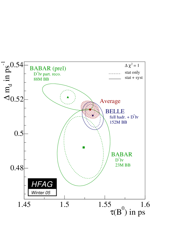
Figure 5: Simultaneous measurements of $\Delta m_{d}$ and $\tau(B^{0})$ [58, 60, 61], after adjustment to a common set of parameters (see text). Statistical and total uncertainties are represented as dashed and solid contours respectively. The average of the three measurements is indicated by a hatched ellipse.

3.3.2 $B^{0}_{s}$ mixing parameters

$C\!P$ violation parameter $|q/p|_{s}$

No measurement or experimental limit exists on $|q/p|_{s}$, except in the form of a relatively weak constraint from CDF on a combination of $|q/p|_{d}$ and $|q/p|_{s}$, $f^{\prime}_{d}\,\chi_{d}(1-|q/p|^{2}_{d})+f^{\prime}_{s}\,\chi_{s}(1-|q/p|^{2}_{s})=0.006\pm 0.017$ [88], using inclusive semileptonic decays of $b$ hadrons. The result is compatible with no $C\!P$ violation in the mixing, an assumption made in all results described below.

Mass difference $\Delta m_{s}$

The time-integrated measurements of $\overline{\chi}$ (see Sec. 3.1.2), when compared to our knowledge of $\chi_{d}$ and the $b$-hadron fractions, indicate that $B^{0}_{s}$ mixing is large, with a value of $\chi_{s}$ close to its maximal possible value of $1/2$. However, the time dependence of this mixing (called $B^{0}_{s}$ oscillations) has not been observed yet, mainly because the period of these oscillations turns out to be so small that it can’t be resolved with the proper-time resolutions achieved so far.

The statistical significance ${\cal S}$ of a $B^{0}_{s}$ oscillation signal can be approximated as [115]

$${\cal S}\approx\sqrt{\frac{N}{2}}\,f_{\rm sig}\,(1-2w)\,\exp{\left(-\left(\Delta m_{s}\sigma_{t}\right)^{2}/2\right)}\,,$$ (45)

where $N$ is the number of selected and tagged $B^{0}_{s}$ candidates, $f_{\rm sig}$ is the fraction of $B^{0}_{s}$ signal in the selected and tagged sample, $w$ is the total mistag probability, and $\sigma_{t}$ is the resolution on proper time. As can be seen, the quantity ${\cal S}$ decreases very quickly as $\Delta m_{s}$ increases: this dependence is controlled by $\sigma_{t}$, which is therefore the most critical parameter for $\Delta m_{s}$ analyses. The method widely used for $B^{0}_{s}$ oscillation searches consists of measuring a $B^{0}_{s}$ oscillation amplitude ${\cal A}$ at several different test values of $\Delta m_{s}$, using a maximum likelihood fit based on the functions of Eq. (35) where the cosine terms have been multiplied by ${\cal A}$. One expects ${\cal A}=1$ at the true value of $\Delta m_{s}$ and to ${\cal A}=0$ at a test value of $\Delta m_{s}$ (far) below the true value. To a good approximation, the statistical uncertainty on ${\cal A}$ is Gaussian and equal to $1/{\cal S}$ [115].

Figure 6: $B^{0}_{s}$-oscillation amplitude spectra, displayed separately for each $B^{0}_{s}$ oscillation analysis. The points and error bars represent the measurements of the amplitude ${\cal A}$ and their total uncertainties $\sigma_{\cal A}$, adjusted to a set of physics parameters common to all analyses (including $f_{s}=0.102\pm 0.014$). Values of $\Delta m_{s}$ where the solid curve (${\cal A}+1.645\,\sigma_{\cal A}$) is below 1 are excluded at 95% CL. The dashed curve shows $1.645\,\sigma_{\cal A}$; the number in parenthesis indicates where this curve is equal to 1, and is a measure of the sensitivity of the analysis. a) ALEPH inclusive lepton [116], b) DELPHI inclusive lepton [122], c) OPAL inclusive lepton and dilepton [123], d) CDF1 $\phi$-$\ell$ [117], e) ALEPH $D_{s}$-$\ell$ [116], f) DELPHI $D_{s}$-$\ell$ [122] and $\phi$-$\ell$ [121], g) OPAL $D_{s}$-$\ell$ [124], h) CDF2 $D_{s}$-$\ell$ (preliminary) [118]. Continuation on Fig. 7).

Figure 7: (continuation of Fig. 6) $B^{0}_{s}$-oscillation amplitude spectra, displayed separately for each $B^{0}_{s}$ oscillation analysis, in the same manner as in Fig. 6. a) ALEPH fully reconstructed $B^{0}_{s}$ [116], b) DELPHI fully reconstructed $B^{0}_{s}$ and $D_{s}$-hadron [72], c) SLD $D_{s}$ +tracks [126], d) CDF2 fully reconstructed $B^{0}_{s}$ (preliminary) [119], f) DELPHI inclusive vertex [98], g) SLD inclusive vertex dipole [125], h) DØ $D_{s}$-$\mu$ (preliminary) [120].

Figure 8: Combined $B^{0}_{s}$-oscillation amplitude spectra, displayed separately for each experiment and collider, in the same manner as in Fig. 6. a) ALEPH [116], b) DELPHI [72, 121, 98, 122], c) OPAL [123, 124], d) LEP [116, 72, 121, 98, 122, 123, 124], e) SLD [126, 125], f) CDF2 [118, 119], g) TEVATRON [117, 118, 119, 120], f) all experiments together.

Figures 6 and 7 show the amplitude spectra obtained by ALEPH [116], CDF [117, 118, 119], D0 [120], DELPHI [98, 121, 72, 122], OPAL [123, 124] and SLD [125, 126]. In each analysis, a particular value of $\Delta m_{s}$ can be excluded at 95% CL if ${\cal A}+1.645\,\sigma_{\cal A}<1$, where $\sigma_{\cal A}$ is the total uncertainty on ${\cal A}$. Because of the proper time resolution, the quantity $\sigma_{\cal A}(\Delta m_{s})$ is an increasing function of $\Delta m_{s}$ (see Eq. (45) which merely models $1/\sigma_{\cal A}(\Delta m_{s})$ since all results are limited by the available statistics). Therefore, if the true value of $\Delta m_{s}$ were infinitely large, one expects to be able to exclude all values of $\Delta m_{s}$ up to $\Delta m_{s}^{\rm sens}$, where $\Delta m_{s}^{\rm sens}$, called here the sensitivity of the analysis, is defined by $1.645\,\sigma_{\cal A}(\Delta m_{s}^{\rm sens})=1$. The most sensitive analyses appear to be the ones based on inclusive lepton samples at LEP, where reasonable statistics is available. Because of their better proper time resolution, the small data samples analyzed inclusively at SLD, as well as the few fully reconstructed $B^{0}_{s}$ decays at LEP, turn out to be also very useful to explore the high $\Delta m_{s}$ region. Recent preliminary analyses are available from CDF and DØ, which presently are the only experiments active in this area.

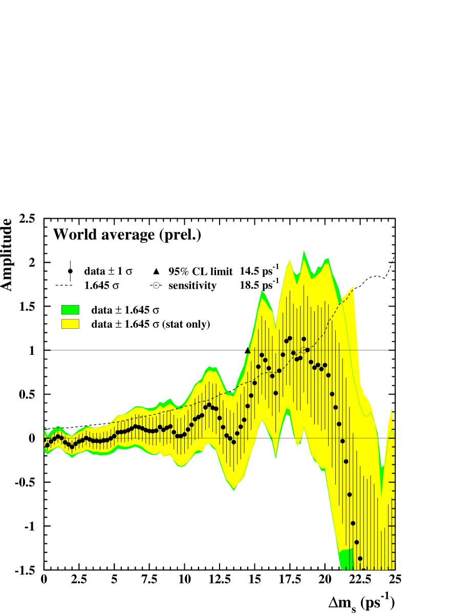
Figure 9: Combined measurements of the $B^{0}_{s}$ oscillation amplitude as a function of $\Delta m_{s}$, including all published results and preliminary results presented at the Winter 2005 conferences [116, 117, 118, 119, 120, 98, 121, 72, 122, 123, 124, 125, 126]. The measurements are dominated by statistical uncertainties. Neighboring points are statistically correlated.

These oscillation searches can easily be combined by averaging the measured amplitudes ${\cal A}$ at each test value of $\Delta m_{s}$. The combined amplitude spectra for the individual experiments are displayed in Fig. 8, and the world average spectrum is displayed in Fig. 9. The individual results have been adjusted to common physics inputs, and all known correlations have been accounted for; in the case of the inclusive analyses, the sensitivities (i.e. the statistical uncertainties on ${\cal A}$), which depend directly through Eq. (45) on the assumed fraction $f_{\rm sig}\sim f_{s}$ of $B^{0}_{s}$ mesons in an unbiased sample of weakly-decaying $b$ hadrons, have also been rescaled to a common average of $f_{s}=0.102\pm 0.014$. The combined sensitivity for 95% CL exclusion of $\Delta m_{s}$ values is found to be $18.5~{}\rm ps^{-1}$. All values of $\Delta m_{s}$ below $14.5~{}\rm ps^{-1}$ are excluded at 95% CL, which we express as

$$\Delta m_{s}>\rm 14.5~{}\rm ps^{-1}~{}at~{}95\%~{}\mbox{CL}\,.$$ (46)

The values between $14.5~{}\rm ps^{-1}$ and $21.7~{}\rm ps^{-1}$ cannot be excluded, because the data is compatible with a signal in this region. However, no deviation from ${\cal A}=0$ is seen in Fig. 9 that would indicate the observation of a signal.

It should be noted that most $\Delta m_{s}$ analyses assume no decay-width difference in the $B^{0}_{s}$ system. Due to the presence of the $\cosh$ terms in Eq. (35), a non-zero value of $\Delta\Gamma_{s}$ would reduce the oscillation amplitude with a small time-dependent factor that would be very difficult to distinguish from time resolution effects.

Convoluting the average $B^{0}_{s}$ lifetime, $1.479\pm 0.044~{}\rm ps$, with the limit of Eq. (46) yields

$$x_{s}=\Delta m_{s}\,\tau(B^{0}_{s})>\rm 21.1~{}at~{}95\%~{}\mbox{CL}\,.$$ (47)

Under the assumption $\Delta\Gamma_{s}=0$, i.e. $y_{s}=\Delta\Gamma_{s}/(2\Gamma_{s})=0$ (and no $C\!P$ violation in the mixing), this is equivalent to

$$\chi_{s}=\frac{x_{s}^{2}+y_{s}^{2}}{2(x_{s}^{2}+1)}>\rm 0.49888~{}at~{}95\%~{}\mbox{CL}\,.$$ (48)

Decay width difference $\Delta\Gamma_{s}$

Definitions and an introduction to $\Delta\Gamma_{s}$ can also be found in Sec. 3.2.4. Neglecting $C\!P$ violation, the mass eigenstates are also $C\!P$ eigenstates, with the long-lived state being $C\!P$-even and the short-lived one being $C\!P$-odd. Information on $\Delta\Gamma_{s}$ can be obtained by studying the proper time distribution of untagged data samples enriched in $B^{0}_{s}$ mesons [64]. In the case of an inclusive $B^{0}_{s}$ selection [44] or a semileptonic $B^{0}_{s}$ decay selection [121, 66, 69], both the short- and long-lived components are present, and the proper time distribution is a superposition of two exponentials with decay constants $\Gamma_{s}\pm\Delta\Gamma_{s}/2$. In principle, this provides sensitivity to both $\Gamma_{s}$ and $(\Delta\Gamma_{s}/\Gamma_{s})^{2}$. Ignoring $\Delta\Gamma_{s}$ and fitting for a single exponential leads to an estimate of $\Gamma_{s}$ with a relative bias proportional to $(\Delta\Gamma_{s}/\Gamma_{s})^{2}$. An alternative approach, which is directly sensitive to first order in $\Delta\Gamma_{s}/\Gamma_{s}$, is to determine the lifetime of $B^{0}_{s}$ candidates decaying to $C\!P$ eigenstates; measurements exist for $B^{0}_{s}\to J/\psi\phi$ [38, 51, 54] and $B^{0}_{s}\to D_{s}^{(*)+}D_{s}^{(*)-}$ [128], which are mostly $C\!P$-even states [129]. However, more recent time-dependent angular analyses of $B^{0}_{s}\to J/\psi\phi$ allow the simultaneous extraction of $\Delta\Gamma_{s}/\Gamma_{s}$ and the $C\!P$-even and $C\!P$-odd amplitudes [130, 131]. An estimate of $\Delta\Gamma_{s}/\Gamma_{s}$ has also been obtained directly from a measurement of the $B^{0}_{s}\to D_{s}^{(*)+}D_{s}^{(*)-}$ branching ratio [128], under the assumption that these decays account for all the $C\!P$-even final states (however, no systematic uncertainty due to this assumption is given, so the average quoted below will not include this estimate).

Table 15: Experimental constraints on $\Delta\Gamma_{s}/\Gamma_{s}$. The upper limits, which have been obtained by the working group, are quoted at the 95% CL.

Experiment	Method	$\Delta\Gamma_{s}/\Gamma_{s}$	Ref.
L3	lifetime of inclusive $b$-sample	$<0.67$	[44]
DELPHI	$\kern 1.79993pt\overline{\kern-1.79993ptB}{}_{s}\to D_{s}^{+}\ell^{-}\overline{\nu_{\ell}}X$, lifetime	$<0.46$	[67]
ALEPH	$B^{0}_{s}\to\phi\phi X$ , ${\cal B}(B^{0}_{s}\to D_{s}^{(*)+}D_{s}^{(*)-})$	$0.26^{+0.30}_{-0.15}$	[128]
ALEPH	$B^{0}_{s}\to\phi\phi X$, lifetime	$0.45^{+0.80}_{-0.49}$	[128]
DELPHI	$\kern 1.79993pt\overline{\kern-1.79993ptB}{}_{s}\to D_{s}^{+}$ hadron, lifetime	$<0.69$	[67]
CDF	$B^{0}_{s}\to J/\psi\phi$, lifetime	$0.33^{+0.45}_{-0.42}$	[38]
CDF	$B^{0}_{s}\to J/\psi\phi$, time-dependent angular analysis	$0.65^{+0.25}_{-0.33}\pm 0.01$	[130]
DØ	$B^{0}_{s}\to J/\psi\phi$, time-dependent angular analysis	$0.21^{+0.33}_{-0.45}$	[131]p
p Preliminary

Measurements quoting $\Delta\Gamma_{s}$ results are listed in Table 15. There is significant correlation between $\Delta\Gamma_{s}/\Gamma_{s}$ and $1/\Gamma_{s}$. In order to combine these measurements, the two-dimensional log-likelihood for each measurement in the $(1/\Gamma_{s},\,\Delta\Gamma_{s}/\Gamma_{s})$ plane is summed and the total normalized with respect to its minimum. The one-sigma contour (corresponding to 0.5 units of log-likelihood greater than the minimum) and 95% contour are found. Inputs as indicated in Table 15 were used in the combination, with the exception of the L3 [44] result since the likelihood for the results was not available, and the ALEPH [128] branching ratio result for the reason given above.

Results of the combination are shown as the one-sigma contour labelled “Direct” in both plots of Fig. 10. Transformation of variables from $(1/\Gamma_{s},\,\Delta\Gamma_{s}/\Gamma_{s})$ space to other pairs of variables such as $(1/\Gamma_{s},\,\Delta\Gamma_{s})$ and $(\tau_{\rm L}=1/\Gamma_{\rm L},\,\tau_{\rm H}=1/\Gamma_{\rm H})$ are also made. The resulting one-sigma contour for the latter is shown in Fig. 10(b).

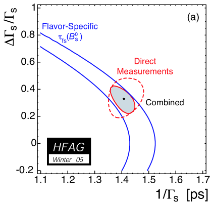
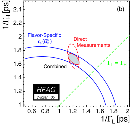
Figure 10: $\Delta\Gamma_{s}$ combination results with one-sigma contours ($\Delta\log\mathcal{L}=0.5$) shown for (a) $\Delta\Gamma_{s}/\Gamma_{s}$ versus $\overline{\tau}(B^{0}_{s})=1/\Gamma_{s}$ and (b) $\tau_{\rm H}=1/\Gamma_{\rm H}$ versus $\tau_{\rm L}=1/\Gamma_{\rm L}$. Contours labelled “Direct” are the result of the combination of most measurements of Table 15, the blue bands are the one-sigma contours due to the world average of flavor-specific measurements, and the shaded region the combination of both. In (b), the diagonal dashed line indicates $\Gamma_{\rm L}=\Gamma_{\rm H}$, i.e., where $\Delta\Gamma_{s}=0$.

Numerical results of the combination of the described inputs of Table 15 are:

$$\Delta\Gamma_{s}/\Gamma_{s} \in [+0.01,+0.59]~{}\mbox{at 95\%~{}\mbox{CL}}\,,$$ (49)

$$\Delta\Gamma_{s}/\Gamma_{s} = +0.35^{+0.12}_{-0.16}\,,$$ (50)

$$\Delta\Gamma_{s} = +0.25^{+0.09}_{-0.11}~{}\rm ps^{-1}\,,$$ (51)

$$\overline{\tau}(B^{0}_{s})=1/\Gamma_{s} = 1.42^{+0.06}_{-0.07}~{}\rm ps\,,$$ (52)

$$1/\Gamma_{\rm L} = \tau_{\rm short}=1.21^{+0.08}_{-0.09}~{}\rm ps\,,$$ (53)

$$1/\Gamma_{\rm H} = \tau_{\rm long}=1.72\pm 0.19~{}\rm ps\,.$$ (54)

Flavor-specific lifetime measurements are of an equal mix of $C\!P$-even and $C\!P$-odd states at time zero, and if a single exponential function is used in the likelihood lifetime fit of such a sample [64],

$$\tau(B^{0}_{s})_{\rm fs}=\frac{1}{\Gamma_{s}}\frac{{1+\left(\frac{\Delta\Gamma_{s}}{2\Gamma_{s}}\right)^{2}}}{{1-\left(\frac{\Delta\Gamma_{s}}{2\Gamma_{s}}\right)^{2}}}.$$ (55)

Using the world average flavor-specific lifetime of Sec. 3.2.4 the one-sigma blue bands shown in Fig. 10 are obtained. Higher-order corrections were checked to be negligible in the combination. When these flavor-specific measurements are combined with the measurements of Table 15, the shaded regions of Fig. 10 are obtained, with numerical results:

$$\Delta\Gamma_{s}/\Gamma_{s} \in [+0.01,+0.59]~{}\mbox{at 95\%~{}\mbox{CL}}\,,$$ (56)

$$\Delta\Gamma_{s}/\Gamma_{s} = +0.33^{+0.09}_{-0.11}\,,$$ (57)

$$\Delta\Gamma_{s} = +0.23\pm 0.08~{}\rm ps^{-1}\,,$$ (58)

$$\overline{\tau}(B^{0}_{s})=1/\Gamma_{s} = 1.405^{+0.043}_{-0.047}~{}\rm ps\,,$$ (59)

$$\rho(\Delta\Gamma_{s}/\Gamma_{s},1/\Delta\Gamma_{s}) = -0.76\,,$$ (60)

$$1/\Gamma_{\rm L} = \tau_{\rm short}=1.21\pm 0.08~{}\rm ps\,,$$ (61)

$$1/\Gamma_{\rm H} = \tau_{\rm long}=1.68^{+0.08}_{-0.09}~{}\rm ps\,.$$ (62)

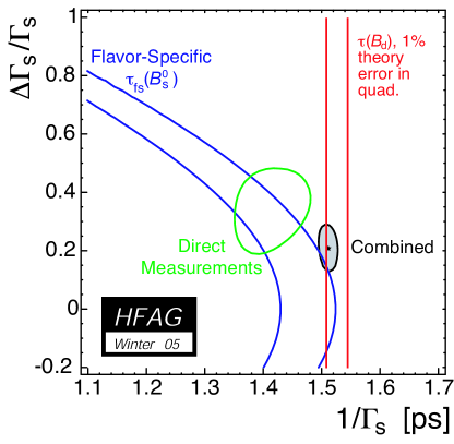
Figure 11: $\Delta\Gamma_{s}$ combination results with one-sigma contours ($\Delta\log\mathcal{L}=0.5$) shown for $\Delta\Gamma_{s}/\Gamma_{s}$ versus $\overline{\tau}(B^{0}_{s})=1/\Gamma_{s}$. The contour labelled “Direct” is the result of the combination of most measurements of Table 15, the blue band is the one-sigma contour due to the world average of flavor-specific measurements, the red vertical band the one-sigma constraint of $\overline{\tau}(B^{0}_{s})=1/\Gamma_{s}=\tau(B^{0})=1/\Gamma_{d}$ (with an additional 1% error added in quadrature), and the shaded region the combination.

The average $B^{0}_{s}$ and $B^{0}$ lifetimes are predicted to be equal within 1% [83, 27] and an informative constraint to apply is to set $\Gamma_{s}=\Gamma_{d}$. The constraint $1/\Gamma_{s}=\tau(B^{0})$ is used, where $\tau(B^{0})=1.528\pm 0.009~{}\rm ps$ is the world average of experimental results, including an additional relative 1% theoretical uncertainty added in quadrature with the indicated error. With this constraint, one obtains the one-sigma contour shown in Fig. 11, and a numerical value of $\Delta\Gamma_{s}/\Gamma_{s}=+0.22^{+0.07}_{-0.09}$. This and the results above can be compared with the theoretical prediction of $\Delta\Gamma_{s}/\Gamma_{s}=0.12\pm 0.05$ [63].

4 Semileptonic $B$ decays

In this edition of the HFAG updates, we present updated values for the total semileptonic branching fraction, the branching fractions ${\cal B}(\overline{B}^{0}\to D^{*+}\ell^{-}\overline{\nu})$ and ${\cal B}(\overline{B}^{0}\to D^{+}\ell^{-}\overline{\nu})$, and the measurements of $F(1)|V_{cb}|$ versus $\rho^{2}$ and $G(1)|V_{cb}|$ versus $\rho^{2}$. For other quantities the reader is referred to the previous HFAG document. [3]

The determination of $|V_{ub}|$ from inclusive decays is the subject of ongoing intense activity in both experiment and theory. HFAG subgroups are currently determining updated values for the heavy quark parameters $m_{b}$ and $\mu_{\pi}^{2}$ based on moments measured in inclusive $\kern 1.79993pt\overline{\kern-1.79993ptB}{}\to X_{c}\ell\overline{\nu}$ and $B\to X_{s}\gamma$ decays. In addition, the theoretical tools have improved [146] and these improvements are being incorporated by the experiments. A comprehensive determination of $|V_{ub}|$ from inclusive decays will be made based on the results presented at the 2005 summer conferences.

Some new measurements of exclusive $B\to X_{u}\ell\overline{\nu}\hbox{ }$ decays were presented at the winter 2005 conferences. A subgroup is working on the averaging of these results and the determination of $|V_{ub}|$ from them. In this article the results are summarized, but no average is quoted.

In the following a detailed description of all parameters and published analyses (including preliminary results) relevant for the determination of the combined results is provided. The description is based on the information available on the web page at

http://www.slac.stanford.edu/xorg/hfag/semi/winter05/winter05.shtml

In the combination of the published results, the central values and errors are rescaled to a common set of input parameters, summarized in Table 16 and provided in the file common.param (accessible from the web page). All measurements with a dependency on any of these parameters are rescaled to the central values given in Table 16, and their error is recalculated based on the error provided in the column “Excursion”. The detailed dependency for each measurement is contained in files (provided by the experiments) accessible from the web page.

Table 16: Common input parameters for the combination of semileptonic $B$ decays. Most of the parameters are taken from Ref. [4]. This table is encoded in the file common.param. The units are picoseconds for lifetimes and percentage for branching fractions.

Parameter	Assumed Value	Excursion	Description
rb	$21.646$	$\pm 0.065$	$R_{b}$
bdst	$1.27$	$\pm 0.021$	${\cal B}(\kern 1.79993pt\overline{\kern-1.79993ptB}{}\to D^{*}\tau\overline{\nu})$
bdsd	$1.62$	$\pm 0.040$	${\cal B}(\kern 1.79993pt\overline{\kern-1.79993ptB}{}\to D^{*}D)$
bdst2	$0.65$	$\pm 0.013$	${\cal B}(b\to D^{*}\tau)$ (OPAL incl)
bdsd2	$4.2$	$\pm 1.5$	${\cal B}(b\to D^{*}D)$ (OPAL incl)
bdsd3	$0.87$	${}^{+0.23}_{-0.19}$	${\cal B}(b\to D^{*}D)$ (DELPHI incl)
xe	$0.702$	$\pm 0.008$	$B$ fragmentation: $\langle E_{B}\rangle/E_{\rm beam}$
bdsi	$17.3$	$\pm 2.0$	${\cal B}(b\to D^{*+}\ \mathrm{incl})$
cdsi	$22.6$	$\pm 1.4$	${\cal B}(c\to D^{*+}\ \mathrm{incl})$
tb0	$1.532$	$\pm 0.009$	$\tau(B^{0})$
tbplus	$1.638$	$\pm 0.011$	$\tau(B^{+})$
tbps	$1.469$	$\pm 0.059$	$\tau(B^{0}_{s})$
fbd	$39.9$	$\pm 1.0$	$B^{0}$ fraction at $\sqrt{s}=m_{Z^{0}}$
fbs	$10.3$	$\pm 1.5$	$B^{0}_{s}$ fraction at $\sqrt{s}=m_{Z^{0}}$
fbar	$10.0$	$\pm 1.7$	Baryon fraction at $\sqrt{s}=m_{Z^{0}}$
dst	$67.7$	$\pm 0.5$	${\cal B}(D^{*+}\to D^{0}\pi^{+})$
dkpp	$9.20$	$\pm 0.6$	${\cal B}(D^{+}\to K^{-}\pi^{+}\pi^{+})$
dkp	$3.80$	$\pm 0.09$	${\cal B}(D^{0}\to K^{-}\pi^{+})$
dkpzp	$13.0$	$\pm 0.8$	${\cal B}(D^{0}\to K^{-}\pi^{+}\pi^{0})$
dkppp	$7.46$	$\pm 0.31$	${\cal B}(D^{0}\to K^{-}\pi^{+}\pi^{+}\pi^{-})$
dkzpp	$2.99$	$\pm 0.18$	${\cal B}(D^{0}\to K^{0}\pi^{+}\pi^{-})$
dkln	$7.0$	$\pm 0.4$	${\cal B}(D^{0}\to K^{-}\ell^{+}\nu)$
dkk	$4.3$	$\pm 0.2$	${\cal B}(D^{0}\to K^{-}K^{+})$
dkx	$1.100$	$\pm 0.025$	$K^{-}\pi^{+}X$ rates
dkox	$0.42$	$\pm 0.05$	${\cal B}(D^{0}\to K^{0}X)$
dnlx	$6.87$	$\pm 0.28$	${\cal B}(D^{0}\to X\ell\overline{\nu})$
dkpcl	$61.2$	$\pm 2.9$	${\cal B}(D^{*0}\to D^{0}\pi^{0})$
dssR	$0.64$	$\pm 0.11$	${\cal B}(b\to D^{**}\ell\overline{\nu})\times{\cal B}(D^{**}\to D^{*+}X)$
fb0	$49.8$	$\pm 0.9$	$f^{00}={\cal B}(\mathchar 28935\relax{(4S)}\to B^{0}\kern 1.79993pt\overline{\kern-1.79993ptB}{}^{0})$
chid	$0.187$	$\pm 0.003$	$\chi_{d}$, time-integrated probability for $B^{0}$ mixing
chi	$0.0930$	$\pm 0.0023$	$\chi=\chi_{d}\times(f^{00}/100)$

4.1 Exclusive Cabibbo-favored decays

Aspects of the phenomenology of exclusive Cabibbo-favored $B$ decays and their use in the determination of $|V_{cb}|$ in the context of Heavy Quark Effective Theory (HQET) are described in many places, e.g., in Ref. [132] and will not be repeated here.

Averages are provided for the branching fractions ${\cal B}(\overline{B}^{0}\to D^{*+}\ell^{-}\overline{\nu})$ plus ${\cal B}(\overline{B}^{0}\to D^{+}\ell^{-}\overline{\nu})$. In addition, averages are provided for $|V_{cb}|F(1)$.vs.$\rho^{2}$, where $F(1)$ and $\rho^{2}$ are the normalization and slope of the form factor at zero recoil in $\overline{B}^{0}\to D^{*+}\ell^{-}\overline{\nu}$ decays, and for the corresponding quantities $|V_{cb}|G(1)$.vs.$\rho^{2}$ in $\overline{B}^{0}\to D^{+}\ell^{-}\overline{\nu}$ decays.

4.1.1 $\overline{B}^{0}\to D^{*+}\ell^{-}\overline{\nu}$

The measurements included in the average, shown in Table 17 are scaled to a consistent set of input parameters and their errors. Therefore some of the (older) measurements are subject to considerable adjustments.

• In order to reduce the dependence on theoretical error estimates, the central values and errors for the form factors $R_{1}$ and $R_{2}$ are taken from the measurement by CLEO [134]. However, all experiments (except for the CLEO [139], the recent DELPHI [140] and the BABAR [141] measurements) quote in their abstracts $F(1)|V_{cb}|$ based on form factors (and their respective errors) from theory. Belle provides a second result evaluated with the CLEO form factors. All other experiments have recalculated $F(1)|V_{cb}|$ to rely on the CLEO form factors. In the future, a substantial improvement in the error associated with form factors is expected by including form factor measurements at the $B$ factories.

• Updates in the branching fractions of $D$ mesons and the production of $D^{**}$ mesons in $B$ decays have generally lead to increased rates for ${\cal B}(\overline{B}^{0}\to D^{*+}\ell^{-}\overline{\nu})$.

• The average $B^{0}$ lifetime has changed considerably since the ALEPH measurement, especially with the much higher precision available at the $B$ factories. This effect is less visible in the other measurements as they are more recent.

• The production of $B^{0}$ mesons at $\sqrt{s}=m_{Z^{0}}$ has a direct impact on all LEP measurements. Adjusting results on the $\mathchar 28935\relax{(4S)}$ for the branching fraction of ${\cal B}(\mathchar 28935\relax{(4S)}\to B^{0}{\kern-1.60004pt\kern 1.79993pt\overline{\kern-1.79993ptB}{}^{0}})\equiv f^{00}$ yields an increase compared to the assumption of $f^{00}=0.5$.

• Many input parameters are now known with a much increased precision—this decreases some of the systematic errors of the rescaled results with respect to the original publication.

The largest correlated errors are the fraction of $B^{0}$ mesons (fbd and fb0, respectively), the form factors $R_{1}(1)$ and $R_{2}(1)$ at zero recoil, $B^{0}$ meson lifetime, branching fractions of $D$ mesons, and the details of $D^{**}$ modeling.

At LEP, the measurements of $\overline{B}^{0}\to D^{*+}\ell^{-}\overline{\nu}$ decays have been done both with “inclusive” analyses based on a partial reconstruction of the $\overline{B}^{0}\to D^{*+}\ell^{-}\overline{\nu}$ decay and a full reconstruction of the exclusive decay. The average branching fraction ${\cal B}(\overline{B}^{0}\to D^{*+}\ell^{-}\overline{\nu})$ is determined in a one-dimensional fit from the measurements provided in Table 17. The statistical correlation between two analyses from the same experiment (DELPHI and OPAL, respectively) is taken into account. Figure 12(a) illustrates the measurements and the resulting average. The $\chi^{2}/{\rm dof}=15.6/7$ corresponds to a 2.9% confidence level, suggesting some caution in interpreting the errors on the average.

Table 17: Average branching fraction ${\cal B}(\overline{B}^{0}\to D^{*+}\ell^{-}\overline{\nu})$ and individual results. See the description in the text for explanations why the published results are lower than the rescaled results.

Experiment	${\cal B}(\overline{B}^{0}\to D^{*+}\ell^{-}\overline{\nu})[\%]$ (rescaled)	${\cal B}(\overline{B}^{0}\to D^{*+}\ell^{-}\overline{\nu})[\%]$ (published)
ALEPH (excl)  [135]	$5.77\pm 0.26_{\rm stat}\pm 0.36_{\rm syst}$	$5.53\pm 0.26_{\rm stat}\pm 0.52_{\rm syst}$
OPAL (excl)  [136]	$5.50\pm 0.19_{\rm stat}\pm 0.39_{\rm syst}$	$5.11\pm 0.19_{\rm stat}\pm 0.49_{\rm syst}$
OPAL (incl)  [136]	$6.19\pm 0.27_{\rm stat}\pm 0.58_{\rm syst}$	$5.92\pm 0.27_{\rm stat}\pm 0.68_{\rm syst}$
DELPHI (incl)  [137]	$5.04\pm 0.13_{\rm stat}\pm 0.36_{\rm syst}$	$4.70\pm 0.13_{\rm stat}\ {}^{+0.36}_{-0.31}\ {}_{\rm syst}$
Belle (excl)  [138]	$4.68\pm 0.23_{\rm stat}\pm 0.42_{\rm syst}$	$4.60\pm 0.23_{\rm stat}\pm 0.40_{\rm syst}$
CLEO (excl)  [139]	$6.28\pm 0.19_{\rm stat}\pm 0.39_{\rm syst}$	$6.09\pm 0.19_{\rm stat}\pm 0.40_{\rm syst}$
DELPHI (excl)  [140]	$5.80\pm 0.22_{\rm stat}\pm 0.46_{\rm syst}$	$5.90\pm 0.22_{\rm stat}\pm 0.50_{\rm syst}$
BABAR (excl)  [141]	$4.81\pm 0.07_{\rm stat}\pm 0.34_{\rm syst}$	$4.90\pm 0.07_{\rm stat}\pm 0.36_{\rm syst}$
Average	$5.34\pm 0.20$	$\chi^{2}/{\rm dof}=15.6/7$

The average for $F(1)|V_{cb}|$ is determined by the two-dimensional combination of the results provided in Table 18. This allows the correlation between $F(1)|V_{cb}|$ and $\rho^{2}$ to be maintained. Figure 13(b) illustrates the average $F(1)|V_{cb}|$ and the measurements included in the average. Figure 13(a) provides a one-dimensional projection for illustrative purposes. The $\chi^{2}/{\rm dof}=30.4/14$ corresponds to a 0.7% confidence level; the errors on the average should be taken with caution (no scale factor is applied).

Table 18: Average of $F(1)|V_{cb}|$ determined in the decay $\overline{B}^{0}\to D^{*+}\ell^{-}\overline{\nu}$ and individual results. The fit for the average has $\chi^{2}/{\rm dof}=30.4/14$. The total correlation between the average $F(1)|V_{cb}|$ and $\rho^{2}$ is 0.59.

Experiment	$F(1)|V_{cb}|[10^{-3}]$ (rescaled)	$\rho^{2}$ (rescaled)
	$F(1)|V_{cb}|[10^{-3}]$ (published)	$\rho^{2}$ (published)
ALEPH (excl)  [135]	$33.7\pm 2.1_{\rm stat}\pm 1.6_{\rm syst}$	$0.75\pm 0.25_{\rm stat}\pm 0.37_{\rm syst}$
	$31.9\pm 1.8_{\rm stat}\pm 1.9_{\rm syst}$	$0.37\pm 0.26_{\rm stat}\pm 0.14_{\rm syst}$
OPAL (incl)  [136]	$38.5\pm 1.2_{\rm stat}\pm 2.4_{\rm syst}$	$1.25\pm 0.14_{\rm stat}\pm 0.39_{\rm syst}$
	$37.5\pm 1.2_{\rm stat}\pm 2.5_{\rm syst}$	$1.12\pm 0.14_{\rm stat}\pm 0.29_{\rm syst}$
OPAL (excl)  [136]	$39.3\pm 1.6_{\rm stat}\pm 1.8_{\rm syst}$	$1.49\pm 0.21_{\rm stat}\pm 0.26_{\rm syst}$
	$36.8\pm 1.6_{\rm stat}\pm 2.0_{\rm syst}$	$1.31\pm 0.21_{\rm stat}\pm 0.16_{\rm syst}$
DELPHI (incl)  [137]	$36.9\pm 1.4_{\rm stat}\pm 2.5_{\rm syst}$	$1.50\pm 0.14_{\rm stat}\pm 0.37_{\rm syst}$
	$35.5\pm 1.4_{\rm stat}\ {}^{+2.3}_{-2.4}{}_{\rm syst}$	$1.34\pm 0.14_{\rm stat}\ {}^{+0.24}_{-0.22}{}_{\rm syst}$
Belle (excl)  [138]	$36.2\pm 1.9_{\rm stat}\pm 1.9_{\rm syst}$	$1.45\pm 0.16_{\rm stat}\pm 0.20_{\rm syst}$
	$35.8\pm 1.9_{\rm stat}\pm 1.9_{\rm syst}$	$1.45\pm 0.16_{\rm stat}\pm 0.20_{\rm syst}$
CLEO (excl)  [139]	$43.8\pm 1.3_{\rm stat}\pm 1.8_{\rm syst}$	$1.61\pm 0.09_{\rm stat}\pm 0.21_{\rm syst}$
	$43.1\pm 1.3_{\rm stat}\pm 1.8_{\rm syst}$	$1.61\pm 0.09_{\rm stat}\pm 0.21_{\rm syst}$
DELPHI (excl)  [140]	$38.8\pm 1.8_{\rm stat}\pm 2.1_{\rm syst}$	$1.32\pm 0.15_{\rm stat}\pm 0.33_{\rm syst}$
	$39.2\pm 1.8_{\rm stat}\pm 2.3_{\rm syst}$	$1.32\pm 0.15_{\rm stat}\pm 0.33_{\rm syst}$
BABAR (excl)  [141]	$35.2\pm 0.3_{\rm stat}\pm 1.6_{\rm syst}$	$1.29\pm 0.03_{\rm stat}\pm 0.27_{\rm syst}$
	$35.5\pm 0.3_{\rm stat}\pm 1.6_{\rm syst}$	$1.29\pm 0.03_{\rm stat}\pm 0.27_{\rm syst}$
Average	$37.6\pm 0.9$	$1.56\pm 0.14$

For a determination of $|V_{cb}|$, the form factor at zero recoil $F(1)$ needs to be computed. A possible choice is $F(1)=0.91\pm 0.04_{\rm theo}$ [142], resulting in

$$|V_{cb}|=(41.3\pm 1.0_{\rm exp}\pm 1.8_{\rm theo})\times 10^{-3}.$$

The value for $F(1)$ and its error is based on a comparison of estimates using OPE sum rules and with an HQET based lattice gauge calculation (see Ref. [142] for more details).

Figure 12: Average branching fraction of exclusive semileptonic $B$ decays. (a) $\overline{B}^{0}\to D^{*+}\ell^{-}\overline{\nu}$ and (b) $\overline{B}^{0}\to D^{+}\ell^{-}\overline{\nu}$.

Figure 13: (a) Illustration of the average $F(1)|V_{cb}|$ and rescaled measurements of exclusive $\overline{B}^{0}\to D^{*+}\ell^{-}\overline{\nu}$  decays determined in a two-dimensional fit. (b) Illustration of $F(1)|V_{cb}|$ vs. $\rho^{2}$. The error ellipses correspond to $\Delta\chi^{2}=1$.

4.1.2 $\overline{B}^{0}\to D^{+}\ell^{-}\overline{\nu}$

The average branching fraction ${\cal B}(\overline{B}^{0}\to D^{+}\ell^{-}\overline{\nu})$ is determined by the combination of the results provided in Table 19. The error sources here are the same as discussed in Sec. 4.1.1, but generally at a higher level due to larger background levels, less stringent kinematic constraints, and larger kinematic suppression at the endpoint. Figure 12(b) illustrates the measurements and the resulting average.

Table 19: Average of the branching fraction ${\cal B}(\overline{B}^{0}\to D^{+}\ell^{-}\overline{\nu})$ and individual results.

Experiment	${\cal B}(\overline{B}^{0}\to D^{+}\ell^{-}\overline{\nu})[\%]$ (rescaled)	${\cal B}(\overline{B}^{0}\to D^{+}\ell^{-}\overline{\nu})[\%]$ (published)
ALEPH   [135]	$2.39\pm 0.20_{\rm stat}\pm 0.52_{\rm syst}$	$2.35\pm 0.20_{\rm stat}\pm 0.44_{\rm syst}$
CLEO   [143]	$2.10\pm 0.13_{\rm stat}\pm 0.18_{\rm syst}$	$2.20\pm 0.16_{\rm stat}\pm 0.19_{\rm syst}$
Belle  [144]	$2.18\pm 0.12_{\rm stat}\pm 0.39_{\rm syst}$	$2.13\pm 0.12_{\rm stat}\pm 0.39_{\rm syst}$
Average	$2.12\pm 0.20$	$\chi^{2}/{\rm dof}=0.3/2$

The average for $G(1)|V_{cb}|$ is determined by the two-dimensional combination of the results provided in Table 20. Figure 14(b) illustrates the average $F(1)|V_{cb}|$ and the measurements included in the average. Figure 14(a) provides a one-dimensional projection for illustrative purposes.

Table 20: Average of $G(1)|V_{cb}|$ determined in the decay $\overline{B}^{0}\to D^{+}\ell^{-}\overline{\nu}$  and individual results. The fit for the average has $\chi^{2}/{\rm dof}=0.3/4$.

Experiment	$G(1)|V_{cb}|[10^{-3}]$ (rescaled)	$\rho^{2}$ (rescaled)
	$G(1)|V_{cb}|[10^{-3}]$ (published)	$\rho^{2}$ (published)
ALEPH  [135]	$39.9\pm 10.0_{\rm stat}\pm 6.5_{\rm syst}$	$1.01\pm 0.98_{\rm stat}\pm 0.38_{\rm syst}$
	$31.1\pm 9.9_{\rm stat}\pm 8.6_{\rm syst}$	$0.20\pm 0.98_{\rm stat}\pm 0.50_{\rm syst}$
CLEO   [143]	$45.1\pm 5.8_{\rm stat}\pm 3.5_{\rm syst}$	$1.27\pm 0.25_{\rm stat}\pm 0.14_{\rm syst}$
	$44.8\pm 6.1_{\rm stat}\pm 3.7_{\rm syst}$	$1.30\pm 0.27_{\rm stat}\pm 0.14_{\rm syst}$
Belle  [144]	$41.2\pm 4.4_{\rm stat}\pm 5.2_{\rm syst}$	$1.12\pm 0.22_{\rm stat}\pm 0.14_{\rm syst}$
	$41.1\pm 4.4_{\rm stat}\pm 5.1_{\rm syst}$	$1.12\pm 0.22_{\rm stat}\pm 0.14_{\rm syst}$
Average	$42.2\pm 3.7$	$1.15\pm 0.16$

For a determination of $|V_{cb}|$, the form factor at zero recoil $G(1)$ needs to be computed. A possible choice is $G(1)=1.04\pm 0.06_{\rm theo}$ [142], resulting in

$$|V_{cb}|=(40.6\pm 3.6_{\rm exp}\pm 2.3_{\rm theo})\times 10^{-3}.$$

Figure 14: (a) Illustration of the average $G(1)|V_{cb}|$ and rescaled measurements of exclusive $\overline{B}^{0}\to D^{+}\ell^{-}\overline{\nu}$  decays determined in a two-dimensional fit. (b) Illustration of $F(1)|V_{cb}|$ vs. $\rho^{2}$. The error ellipses correspond to $\Delta\chi^{2}=1$.

4.2 Inclusive Cabibbo-favored decays

Aspects of the theory and phenomenology of inclusive Cabibbo-favored $B$ decays and their use in the determination of $|V_{cb}|$ in the context of the Heavy Quark Expansion (HQE), an Operator Product Expansion based on HQET, are described in many places (see, e.g., Ref. [145] and references therein).

An updated average for the total semileptonic branching fraction ${\cal B}(\kern 1.79993pt\overline{\kern-1.79993ptB}{}\to X\ell\overline{\nu})$ is provided here. In future compilations HFAG will provide averages of moments of the electron and hadron spectra in inclusive semileptonic decays, and perform global fits of these moments to OPE calculations to extract $|V_{cb}|$ and HQE parameters. At present several groups have published these global fits [153, 155, 156, 157].

4.2.1 Total semileptonic branching fraction

The measurements of the total semileptonic branching fraction ${\cal B}(b\to X\ell\overline{\nu})$ at LEP (see, e.g., Ref [4] or Ref. [147]) represent a different analysis class with a more explicit model dependence than the (lepton-)tagged analyses used at the $\mathchar 28935\relax{(4S)}$. Therefore the LEP measurements are not used in the averages computed here.

The average for the total branching fraction ${\cal B}(\kern 1.79993pt\overline{\kern-1.79993ptB}{}\to X\ell\overline{\nu})$ is determined by the combination of the results provided in Table 21. In this average, the extrapolation of the measured rate to the total decay rate is performed by each experiment, usually with a fit of several components to the experimental spectrum. In the two most precise measurements [156, 153], the extrapolation is part of the HQE fit to electron momentum and hadronic invariant mass moments in $\kern 1.79993pt\overline{\kern-1.79993ptB}{}\to X_{c}\ell\overline{\nu}$ decays.

Table 21: Average of the total semileptonic branching fractions ${\cal B}(\kern 1.79993pt\overline{\kern-1.79993ptB}{}\to X\ell\overline{\nu})$ determined in tagged measurements on the $\mathchar 28935\relax{(4S)}$.

Experiment	${\cal B}_{tot}(\kern 1.79993pt\overline{\kern-1.79993ptB}{}\to X\ell\overline{\nu})[\%]$ (rescaled)	${\cal B}_{tot}(\kern 1.79993pt\overline{\kern-1.79993ptB}{}\to X\ell\overline{\nu})[\%]$ (published)
ARGUS ($\ell$-tag)  [148]	$9.77\pm 0.50\pm 0.39$	$9.70\pm 0.50\pm 0.60$
BABAR ($B_{reco}$-tag)  [149]	$10.40\pm 0.50\pm 0.46$	$10.40\pm 0.50\pm 0.46$
Belle ($\ell$-tag)  [150]	$10.98\pm 0.12\pm 0.50$	$10.90\pm 0.12\pm 0.49$
BABAR ($e$-tag HQE)  [156]	$10.87\pm 0.06\pm 0.16$	$10.83\pm 0.06\pm 0.16$
Belle ($B_{reco}$-tag)  [152]	$11.19\pm 0.20\pm 0.31$	$11.19\pm 0.20\pm 0.31$
CLEO ($\ell$-tag HQE)  [153]	$10.95\pm 0.09\pm 0.24$	$10.91\pm 0.09\pm 0.24$
Average	$10.95\pm 0.15$	$\chi^{2}/{\rm dof}=5.0/5$

4.3 Exclusive Cabibbo-suppressed decays

Here we list results on exclusive determinations of $|V_{ub}|$. An average of (these) exclusive $b\to u\ell\overline{\nu}$ results is envisioned for the future. The measurements are separated into two classes: a first one averaging over the entire $q^{2}$ range (shown in Table 22), and a second class, where the decay rate is measured differentially in (few) bins of $q^{2}$ (shown in Table 23).

Table 22: Summary of exclusive determinations of ${\cal B}(\kern 1.79993pt\overline{\kern-1.79993ptB}{}\to X\ell\overline{\nu})$ and $|V_{ub}|$ using the entire $q^{2}$ range. The errors quoted on $|V_{ub}|$ correspond to statistical, experimental systematic and theoretical systematic, respectively.

Experiment	Mode	${\cal B}[10^{-4}]$	$|V_{ub}|$ $[10^{-3}]$ (rescaled)
CLEO   [158]	$B^{0}\to\rho^{-}\ell^{+}\nu$	$2.69\pm 0.41\ {}^{+0.35}_{-0.40}\pm 0.50$	$3.24\pm 0.25\ {}^{+0.21}_{-0.24}\pm 0.58$
BABAR  [159]	$B^{0}\to\rho^{-}\ell^{+}\nu$	$3.29\pm 0.42\pm 0.47\pm 0.60$	$3.59\pm 0.23\pm 0.26\pm 0.66$
Belle  [161]	$B^{+}\to\omega\ell^{+}\nu$	$1.3\pm 0.4\pm 0.2\pm 0.3$	$3.1\pm 0.2\pm 0.2\pm 0.6$
BABAR  [160]	$B^{+}\to\pi^{0}\ell^{+}\nu$	$1.80\pm 0.37\pm 0.23$

Table 23: Summary of exclusive determinations of ${\cal B}(\kern 1.79993pt\overline{\kern-1.79993ptB}{}\to X\ell\overline{\nu})$ and $|V_{ub}|$ binned in $q^{2}$. The errors quoted on $|V_{ub}|$ correspond to statistical, experimental systematic, theoretical systematic, and signal form-factor shape and normalization, respectively.

Experiment	Mode	${\cal B}[10^{-4}]$	$|V_{ub}|$ $[10^{-3}]$ (rescaled)
CLEO   [163]	$B^{0}\to\pi^{-}\ell^{+}\nu$	$1.33\pm 0.18\pm 0.11\pm 0.01\pm 0.07$	$2.88\pm 0.55\pm 0.30\ {}^{+0.45}_{-0.35}\pm 0.18$
Belle  [164]	$B^{0}\to\pi^{-}\ell^{+}\nu$	$1.76\pm 0.28\ \pm 0.20\pm 0.03$	$3.90\pm 0.71\pm 0.23\ {}^{+0.62}_{-0.48}$
BABAR  [165]	$B^{0}\to\pi^{-}\ell^{+}\nu$	$1.46\pm 0.27\ \pm 0.28$
BABAR  [162]	$B^{0}\to\pi-\ell^{+}\nu$	$1.38\pm 0.10\pm 0.18\pm 0.08$	$3.82\pm 0.14\pm 0.24\pm 0.66$
BABAR  [160]	$B^{0}\to\pi-\ell^{+}\nu$	$1.03\pm 0.25\pm 0.13$
CLEO   [163]	$B^{0}\to\rho^{-}\ell^{+}\nu$	$2.17\pm 0.34\ {}^{+0.47}_{-0.54}\pm 0.41\pm 0.01$	$3.34\pm 0.32\ {}^{+0.27}_{-0.36}\ {}^{+0.50}_{-0.40}$
Belle  [164]	$B^{0}\to\rho^{-}\ell^{+}\nu$	$2.54\pm 0.78\ \pm 0.85\pm 0.30$
BABAR  [162]	$B^{0}\to\rho-\ell^{+}\nu$	$2.14\pm 0.21\pm 0.51\pm 0.28$

4.4 Inclusive Cabibbo-suppressed decays

Since the last HFAG update, there has been considerable change in this area. The theoretical tools have been updated, [146] and the use of HQE parameters determined from global fits to $\kern 1.79993pt\overline{\kern-1.79993ptB}{}\to X_{c}\ell\overline{\nu}$ moments as input to shape function parameterizations is now established. A bit more time is needed, however, to integrate these changes into an updated average value for $|V_{ub}|$. Preliminary results shown at the CKM2005 workshop [166] suggest that a substantial downward shift in $|V_{ub}|$ can be expected.

5 Measurements related to Unitarity Triangle angles

The charge of the “$C\!P(t)$ and Unitarity Triangle angles” group is to provide averages of measurements related (mostly) to the angles of the Unitarity Triangle (UT). To date, most of the measurements that can be used to obtain model-independent information on the UT angles come from time-dependent $C\!P$ asymmetry analyses. In cases where considerable theoretical input is required to extract the fundamental quantities, no attempt is made to do so at this stage. However, straightforward interpretations of the averages are given, where possible.

In Sec. 5.1 a brief introduction to the relevant phenomenology is given. In Sec. 5.2 an attempt is made to clarify the various different notations in use. In Sec. 5.3 the common inputs to which experimental results are rescaled in the averaging procedure are listed. We also briefly introduce the treatment of experimental errors. In the remainder of this section, the experimental results and their averages are given, divided into subsections based on the underlying quark-level decays.

5.1 Introduction

The Standard Model Cabibbo-Kobayashi-Maskawa (CKM) quark mixing matrix ${V}$ must be unitary. A $3\times 3$ unitary matrix has four free parameters, and these are conventionally written by the product of three (complex) rotation matrices [167], where the rotations are characterized by the Euler angles $\theta_{12}$, $\theta_{13}$ and $\theta_{23}$, which are the mixing angles between the generations, and one overall phase $\delta$,

$${V}=\left(\begin{array}[]{ccc}V_{ud}&V_{us}&V_{ub}\\ V_{cd}&V_{cs}&V_{cb}\\ V_{td}&V_{ts}&V_{tb}\\ \end{array}\right)=\left(\begin{array}[]{ccc}c_{12}c_{13}&s_{12}c_{13}&s_{13}e^{-i\delta}\\ -s_{12}c_{23}-c_{12}s_{23}s_{13}e^{i\delta}&c_{12}c_{23}-s_{12}s_{23}s_{13}e^{i\delta}&s_{23}c_{13}\\ s_{12}s_{23}-c_{12}c_{23}s_{13}e^{i\delta}&-c_{12}s_{23}-s_{12}c_{23}s_{13}e^{i\delta}&c_{23}c_{13}\end{array}\right)$$ (63)

where $c_{ij}=\cos\theta_{ij}$, $s_{ij}=\sin\theta_{ij}$ for $i<j=1,2,3$.

Following the observation of a hierarchy between the different matrix elements, the Wolfenstein parameterization [168] is an expansion of ${V}$ in terms of the four real parameters $\lambda$ (the expansion parameter), $A$, $\rho$ and $\eta$. Defining to all orders in $\lambda$ [169]

$$s_{12} \equiv \lambda,$$

$$s_{23} \equiv A\lambda^{2},$$ (64)

$$s_{13}e^{-i\delta} \equiv A\lambda^{3}(\rho-i\eta),$$

and inserting these into the representation of Eq. (63), unitarity of the CKM matrix is achieved to all orders. A Taylor expansion of ${V}$ leads to the familiar approximation

$${V}=\left(\begin{array}[]{ccc}1-\lambda^{2}/2&\lambda&A\lambda^{3}(\rho-i\eta)\\ -\lambda&1-\lambda^{2}/2&A\lambda^{2}\\ A\lambda^{3}(1-\rho-i\eta)&-A\lambda^{2}&1\\ \end{array}\right)+{\cal O}\left(\lambda^{4}\right).$$ (65)

The non-zero imaginary part of the CKM matrix, which is the origin of $C\!P$ violation in the Standard Model, is encapsulated in a non-zero value of $\eta$.

The unitarity relation ${V}^{\dagger}{V}={\mathit{1}}$ results in nine expressions which can be written $\sum_{i=u,c,t}V^{*}_{ij}V_{ik}=\delta_{jk}$, where $\delta_{jk}$ is the Kronecker symbol. Of the off-diagonal expressions ($j\neq k$), three can be trivially transformed into the other three (under $j\leftrightarrow k$), leaving six relations, in which three complex numbers sum to zero, which therefore can be expressed as triangles in the complex plane.

One of these,

$$V_{ud}V^{*}_{ub}+V_{cd}V^{*}_{cb}+V_{td}V^{*}_{tb}=0,$$ (66)

is specifically related to $B$ decays. The three terms in Eq. (66) are of the same order (${\cal O}\left(\lambda^{3}\right)$), and this relation is commonly known as the Unitarity Triangle. For presentational purposes, it is convenient to rescale the triangle by $(V_{cd}V^{*}_{cb})^{-1}$, as shown in Fig. 15.

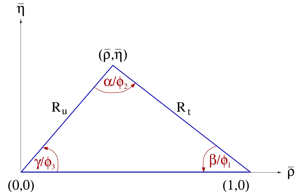
Figure 15: The Unitarity Triangle.

Two popular naming conventions for the UT angles exist in the literature:

$$\alpha\equiv\phi_{2}=\arg\left[-\frac{V_{td}V_{tb}^{*}}{V_{ud}V_{ub}^{*}}\right],\hskip 14.22636pt\beta\equiv\phi_{1}=\arg\left[-\frac{V_{cd}V_{cb}^{*}}{V_{td}V_{tb}^{*}}\right],\hskip 14.22636pt\gamma\equiv\phi_{3}=\arg\left[-\frac{V_{ud}V_{ub}^{*}}{V_{cd}V_{cb}^{*}}\right].$$

In this document the $\left(\alpha,\beta,\gamma\right)$ set is used.

The apex of the Unitarity Triangle is given by the following definition [169]

$$\overline{\rho}+i\overline{\eta}\;\equiv\;-\frac{V_{ud}V_{ub}^{*}}{V_{cd}V_{cb}^{*}}=(\rho+i\eta)(1-\frac{1}{2}\lambda^{2})+{\cal O}(\lambda^{4}).$$ (67)

The sides $R_{u}$ and $R_{t}$ of the Unitarity Triangle (the third side being normalized to unity) are given by

$$R_{u} = \left|\frac{V_{ud}V_{ub}^{*}}{V_{cd}V_{cb}^{*}}\right|\;=\;\sqrt{\overline{\rho}^{2}+\overline{\eta}^{2}},$$ (68)

$$R_{t} = \left|\frac{V_{td}V_{tb}^{*}}{V_{cd}V_{cb}^{*}}\right|\;=\;\sqrt{(1-\overline{\rho})^{2}+\overline{\eta}^{2}}.$$ (69)

5.2 Notations

Several different notations for $C\!P$ violation parameters are commonly used. This section reviews those found in the experimental literature, in the hope of reducing the potential for confusion, and to define the frame that is used for the averages.

In some cases, when $B$ mesons decay into multibody final states via broad resonances ($\rho$, $K^{*}$, etc.), the experiments ignore interference effects in the analyses. This is referred to as the quasi-two-body (Q2B) approximation in the following.

5.2.1 $C\!P$ asymmetries

The $C\!P$ asymmetry is defined as the difference between the rate involving a $b$ quark and that involving a $\overline{b}$ quark, divided by the sum. For example, the partial rate (or charge) asymmetry for a charged $B$ decay would be given as

$${\cal A}_{f}\;\equiv\;\frac{\Gamma(B^{-}\to f)-\Gamma(B^{+}\to\overline{f})}{\Gamma(B^{-}\to f)+\Gamma(B^{+}\to\overline{f})}.$$ (70)

5.2.2 Time-dependent $C\!P$ asymmetries in decays to $C\!P$ eigenstates

If the amplitudes for $B^{0}$ and $\kern 1.79993pt\overline{\kern-1.79993ptB}{}^{0}$ to decay to a final state $f$, which is a $C\!P$ eigenstate with eigenvalue ${\eta_{f}}$, are given by $A_{f}$ and $\kern 1.79993pt\overline{\kern-1.79993ptA}{}_{f}$, respectively, then the decay distributions for neutral $B$ mesons, with known flavour at time $\Delta t=0$, are given by

$$\Gamma_{\kern 1.25995pt\overline{\kern-1.25995ptB}{}^{0}\to f}(\Delta t) = \frac{e^{-|\Delta t|/\tau(B^{0})}}{4\tau(B^{0})}\left[1+\frac{2\,{\rm Im}(\lambda_{f})}{1+|\lambda_{f}|^{2}}\sin(\Delta m\Delta t)-\frac{1-|\lambda_{f}|^{2}}{1+|\lambda_{f}|^{2}}\cos(\Delta m\Delta t)\right],$$ (71)

$$\Gamma_{B^{0}\to f}(\Delta t) = \frac{e^{-|\Delta t|/\tau(B^{0})}}{4\tau(B^{0})}\left[1-\frac{2\,{\rm Im}(\lambda_{f})}{1+|\lambda_{f}|^{2}}\sin(\Delta m\Delta t)+\frac{1-|\lambda_{f}|^{2}}{1+|\lambda_{f}|^{2}}\cos(\Delta m\Delta t)\right].$$ (72)

Here $\lambda_{f}=\frac{q}{p}\frac{\kern 1.25995pt\overline{\kern-1.25995ptA}{}_{f}}{A_{f}}$ contains terms related to $B^{0}$-$\kern 1.79993pt\overline{\kern-1.79993ptB}{}^{0}$ mixing and to the decay amplitude (the eigenstates of the effective Hamiltonian in the $B^{0}{\kern-1.60004pt\kern 1.79993pt\overline{\kern-1.79993ptB}{}^{0}}$ system are $\left|B_{\pm}\right>=p\left|B^{0}\right>\pm q\left|\kern 1.79993pt\overline{\kern-1.79993ptB}{}^{0}\right>$). This formulation assumes $C\!PT$ invariance, and neglects possible lifetime differences in the neutral $B$ meson system. The time-dependent $C\!P$ asymmetry, again defined as the difference between the rate involving a $b$ quark and that involving a $\overline{b}$ quark, is then given by

$${\cal A}_{f}\left(\Delta t\right)\;\equiv\;\frac{\Gamma_{\kern 1.25995pt\overline{\kern-1.25995ptB}{}^{0}\to f}(\Delta t)-\Gamma_{B^{0}\to f}(\Delta t)}{\Gamma_{\kern 1.25995pt\overline{\kern-1.25995ptB}{}^{0}\to f}(\Delta t)+\Gamma_{B^{0}\to f}(\Delta t)}\;=\;\frac{2\,{\rm Im}(\lambda_{f})}{1+|\lambda_{f}|^{2}}\sin(\Delta m\Delta t)-\frac{1-|\lambda_{f}|^{2}}{1+|\lambda_{f}|^{2}}\cos(\Delta m\Delta t).$$ (73)

While the coefficient of the $\sin(\Delta m\Delta t)$ term in Eq. (73) is everywhere denoted $S_{f}$:

$$S_{f}\;\equiv\;\frac{2\,{\rm Im}(\lambda_{f})}{1+\left|\lambda_{f}\right|^{2}},$$ (74)

different notations are in use for the coefficient of the $\cos(\Delta m\Delta t)$ term:

$$C_{f}\;\equiv\;-A_{f}\;\equiv\;\frac{1-\left|\lambda_{f}\right|^{2}}{1+\left|\lambda_{f}\right|^{2}}.$$ (75)

The $C$ notation is used by the BABAR  collaboration (see e.g. [179]), and also in this document. The $A$ notation is used by the Belle collaboration (see e.g. [61]).

Neglecting effects due to $C\!P$ violation in mixing (i.e., taking $|q/p|=1$), if the decay amplitude contains terms with a single weak phase then $\left|\lambda_{f}\right|=1$ and one finds $S_{f}=-{\eta_{f}}\sin(\phi_{\rm mix}+\phi_{\rm dec})$, $C_{f}=0$, where $\phi_{\rm mix}=\arg(q/p)$ and $\phi_{\rm dec}=\arg(\kern 1.79993pt\overline{\kern-1.79993ptA}{}_{f}/A_{f})$. Note that $\phi_{\rm mix}\approx 2\beta$ in the Standard Model (in the usual phase convention). If amplitudes with different weak phases contribute to the decay, no clean interpretation of $S_{f}$ is possible. If the decay amplitudes have in addition different $C\!P$ conserving strong phases, then $\left|\lambda_{f}\right|\neq 1$ and no clean interpretation is possible. The coefficient of the cosine term becomes non-zero, indicating direct $C\!P$ violation. The sign of $A_{f}$ as defined above is consistent with that of ${\cal A}_{f}$ in Eq. (70).

5.2.3 Time-dependent $C\!P$ asymmetries in decays to vector-vector final states

Consider $B$ decays to states consisting of two vector particles, such as ${J\mskip-3.0mu/\mskip-2.0mu\psi\mskip 2.0mu}K^{*0}(\to K^{0}_{\scriptscriptstyle S}\pi^{0})$, $D^{*+}D^{*-}$ and $\rho^{+}\rho^{-}$, which are eigenstates of charge conjugation but not of parity. In fact, for such a system, there are three possible final states; in the helicity basis these can be written $h_{-1},h_{0},h_{+1}$. The $h_{0}$ state is an eigenstate of parity, and hence of $C\!P$; however, $C\!P$ transforms $h_{+1}\leftrightarrow h_{-1}$ (up to an unobservable phase). In the transversity basis, these states are transformed into $h_{\parallel}=(h_{+1}+h_{-1})/2$ and $h_{\perp}=(h_{+1}-h_{-1})/2$. In this basis all three states are $C\!P$ eigenstates, and $h_{\perp}$ has the opposite $C\!P$ to the others.

The amplitudes to these states are usually given by $A_{0,\perp,\parallel}$ (here we use a normalization such that $|A_{0}|^{2}+|A_{\perp}|^{2}+|A_{\parallel}|^{2}=1$). Then the effective $C\!P$ of the vector-vector state is known if $|A_{\perp}|^{2}$ is measured. An alternative strategy is to measure just the longitudinally polarized component, $|A_{0}|^{2}$ (sometimes denoted by $f_{\rm long}$), which allows a limit to be set on the effective $C\!P$ since $|A_{\perp}|^{2}\leq|A_{\perp}|^{2}+|A_{\parallel}|^{2}=1-|A_{0}|^{2}$. The most complete treatment for neutral $B$ decays to vector-vector final states is time-dependent angular analysis (also known as time-dependent transversity analysis). In such an analysis, the interference between the $C\!P$ even and $C\!P$ odd states provides additional sensitivity to the weak and strong phases involved.

5.2.4 Time-dependent $C\!P$ asymmetries in decays to non-$C\!P$ eigenstates

Consider a non-$C\!P$ eigenstate $f$, and its conjugate $\overline{f}$. For neutral $B$ decays to these final states, there are four amplitudes to consider: those for $B^{0}$ to decay to $f$ and $\overline{f}$ ($A_{f}$ and $A_{\overline{f}}$, respectively), and the equivalents for $\kern 1.79993pt\overline{\kern-1.79993ptB}{}^{0}$ ($\kern 1.79993pt\overline{\kern-1.79993ptA}{}_{f}$ and $\kern 1.79993pt\overline{\kern-1.79993ptA}{}_{\overline{f}}$). If $C\!P$ is conserved in the decay, then $A_{f}=\kern 1.79993pt\overline{\kern-1.79993ptA}{}_{\overline{f}}$ and $A_{\overline{f}}=\kern 1.79993pt\overline{\kern-1.79993ptA}{}_{f}$.

The time-dependent decay distributions can be written in many different ways. Here, we follow Sec. 5.2.2 and define $\lambda_{f}=\frac{q}{p}\frac{\kern 1.25995pt\overline{\kern-1.25995ptA}{}_{f}}{A_{f}}$ and $\lambda_{\overline{f}}=\frac{q}{p}\frac{\kern 1.25995pt\overline{\kern-1.25995ptA}{}_{\overline{f}}}{A_{\overline{f}}}$. The time-dependent $C\!P$ asymmetries then follow Eq. (73):

$${\cal A}_{f}(\Delta t)\;\equiv\;\frac{\Gamma_{\kern 1.25995pt\overline{\kern-1.25995ptB}{}^{0}\to f}(\Delta t)-\Gamma_{B^{0}\to f}(\Delta t)}{\Gamma_{\kern 1.25995pt\overline{\kern-1.25995ptB}{}^{0}\to f}(\Delta t)+\Gamma_{B^{0}\to f}(\Delta t)} = S_{f}\sin(\Delta m\Delta t)-C_{f}\cos(\Delta m\Delta t),$$ (76)

$${\cal A}_{\overline{f}}(\Delta t)\;\equiv\;\frac{\Gamma_{\kern 1.25995pt\overline{\kern-1.25995ptB}{}^{0}\to\overline{f}}(\Delta t)-\Gamma_{B^{0}\to\overline{f}}(\Delta t)}{\Gamma_{\kern 1.25995pt\overline{\kern-1.25995ptB}{}^{0}\to\overline{f}}(\Delta t)+\Gamma_{B^{0}\to\overline{f}}(\Delta t)} = S_{\overline{f}}\sin(\Delta m\Delta t)-C_{\overline{f}}\cos(\Delta m\Delta t),$$ (77)

with the definitions of the parameters $C_{f}$, $S_{f}$, $C_{\overline{f}}$ and $S_{\overline{f}}$, following Eqs. (74) and (75).

The time-dependent decay rates are given by

$$\Gamma_{\kern 1.25995pt\overline{\kern-1.25995ptB}{}^{0}\to f}(\Delta t) = \frac{e^{-\left|\Delta t\right|/\tau(B^{0})}}{8\tau(B^{0})}(1+\langle{\cal A}_{f\overline{f}}\rangle)\left\{1+S_{f}\sin(\Delta m\Delta t)-C_{f}\cos(\Delta m\Delta t)\right\},$$ (78)

$$\Gamma_{B^{0}\to f}(\Delta t) = \frac{e^{-\left|\Delta t\right|/\tau(B^{0})}}{8\tau(B^{0})}(1+\langle{\cal A}_{f\overline{f}}\rangle)\left\{1-S_{f}\sin(\Delta m\Delta t)+C_{f}\cos(\Delta m\Delta t)\right\},$$ (79)

$$\Gamma_{\kern 1.25995pt\overline{\kern-1.25995ptB}{}^{0}\to\overline{f}}(\Delta t) = \frac{e^{-\left|\Delta t\right|/\tau(B^{0})}}{8\tau(B^{0})}(1-\langle{\cal A}_{f\overline{f}}\rangle)\left\{1+S_{\overline{f}}\sin(\Delta m\Delta t)-C_{\overline{f}}\cos(\Delta m\Delta t)\right\},$$ (80)

$$\Gamma_{B^{0}\to\overline{f}}(\Delta t) = \frac{e^{-\left|\Delta t\right|/\tau(B^{0})}}{8\tau(B^{0})}(1-\langle{\cal A}_{f\overline{f}}\rangle)\left\{1-S_{\overline{f}}\sin(\Delta m\Delta t)+C_{\overline{f}}\cos(\Delta m\Delta t)\right\},$$ (81)

where the time-independent parameter $\langle{\cal A}_{f\overline{f}}\rangle$ represents an overall asymmetry in the production of the $f$ and $\overline{f}$ final states,

$$\langle{\cal A}_{f\overline{f}}\rangle=\frac{\left(\left|A_{f}\right|^{2}+\left|\kern 1.79993pt\overline{\kern-1.79993ptA}{}_{f}\right|^{2}\right)-\left(\left|A_{\overline{f}}\right|^{2}+\left|\kern 1.79993pt\overline{\kern-1.79993ptA}{}_{\overline{f}}\right|^{2}\right)}{\left(\left|A_{f}\right|^{2}+\left|\kern 1.79993pt\overline{\kern-1.79993ptA}{}_{f}\right|^{2}\right)+\left(\left|A_{\overline{f}}\right|^{2}+\left|\kern 1.79993pt\overline{\kern-1.79993ptA}{}_{\overline{f}}\right|^{2}\right)}.$$ (82)

Assuming $|q/p|=1$, the parameters $C_{f}$ and $C_{\overline{f}}$ can also be written in terms of the decay amplitudes as follows:

$$C_{f}=\frac{\left|A_{f}\right|^{2}-\left|\kern 1.79993pt\overline{\kern-1.79993ptA}{}_{f}\right|^{2}}{\left|A_{f}\right|^{2}+\left|\kern 1.79993pt\overline{\kern-1.79993ptA}{}_{f}\right|^{2}}\hskip 14.22636pt{\rm and}\hskip 14.22636ptC_{\overline{f}}=\frac{\left|A_{\overline{f}}\right|^{2}-\left|\kern 1.79993pt\overline{\kern-1.79993ptA}{}_{\overline{f}}\right|^{2}}{\left|A_{\overline{f}}\right|^{2}+\left|\kern 1.79993pt\overline{\kern-1.79993ptA}{}_{\overline{f}}\right|^{2}},$$ (83)

giving asymmetries in the decay amplitudes of $B^{0}$ and $\kern 1.79993pt\overline{\kern-1.79993ptB}{}^{0}$ to the final states $f$ and $\overline{f}$ respectively. In this notation, the direct $C\!P$ invariance conditions are $\langle{\cal A}_{f\overline{f}}\rangle=0$ and $C_{f}=-C_{\overline{f}}$. Note that $C_{f}$ and $C_{\overline{f}}$ are typically non-zero; e.g., for a flavour-specific final state, $\kern 1.79993pt\overline{\kern-1.79993ptA}{}_{f}=A_{\overline{f}}=0$ ($A_{f}=\kern 1.79993pt\overline{\kern-1.79993ptA}{}_{\overline{f}}=0$), they take the values $C_{f}=-C_{\overline{f}}=1$ ($C_{f}=-C_{\overline{f}}=-1$).

The coefficients of the sine terms contain information about the weak phase. In the case that each decay amplitude contains only a single weak phase (i.e., no direct $C\!P$ violation), these terms can be written

$$S_{f}=\frac{-2\left|A_{f}\right|\left|\kern 1.79993pt\overline{\kern-1.79993ptA}{}_{f}\right|\sin(\phi_{\rm mix}+\phi_{\rm dec}-\delta_{f})}{\left|A_{f}\right|^{2}+\left|\kern 1.79993pt\overline{\kern-1.79993ptA}{}_{f}\right|^{2}}\hskip 14.22636pt{\rm and}\hskip 14.22636ptS_{\overline{f}}=\frac{-2\left|A_{\overline{f}}\right|\left|\kern 1.79993pt\overline{\kern-1.79993ptA}{}_{\overline{f}}\right|\sin(\phi_{\rm mix}+\phi_{\rm dec}+\delta_{f})}{\left|A_{\overline{f}}\right|^{2}+\left|\kern 1.79993pt\overline{\kern-1.79993ptA}{}_{\overline{f}}\right|^{2}},$$ (84)

where $\delta_{f}$ is the strong phase difference between the decay amplitudes. If there is no $C\!P$ violation, the condition $S_{f}=-S_{\overline{f}}$ holds. If amplitudes with different weak and strong phases contribute, no clean interpretation of $S_{f}$ and $S_{\overline{f}}$ is possible.

Since two of the $C\!P$ invariance conditions are $C_{f}=-C_{\overline{f}}$ and $S_{f}=-S_{\overline{f}}$, there is motivation for a rotation of the parameters:

$$S_{f\overline{f}}=\frac{S_{f}+S_{\overline{f}}}{2},\hskip 11.38109pt\Delta S_{f\overline{f}}=\frac{S_{f}-S_{\overline{f}}}{2},\hskip 11.38109ptC_{f\overline{f}}=\frac{C_{f}+C_{\overline{f}}}{2},\hskip 11.38109pt\Delta C_{f\overline{f}}=\frac{C_{f}-C_{\overline{f}}}{2}.$$ (85)

With these parameters, the $C\!P$ invariance conditions become $S_{f\overline{f}}=0$ and $C_{f\overline{f}}=0$. The parameter $\Delta C_{f\overline{f}}$ gives a measure of the “flavour-specificity” of the decay: $\Delta C_{f\overline{f}}=\pm 1$ corresponds to a completely flavour-specific decay, in which no interference between decays with and without mixing can occur, while $\Delta C_{f\overline{f}}=0$ results in maximum sensitivity to mixing-induced $C\!P$ violation. The parameter $\Delta S_{f\overline{f}}$ is related to the strong phase difference between the decay amplitudes of $B^{0}$ to $f$ and to $\overline{f}$. We note that the observables of Eq. (85) exhibit experimental correlations (typically of $\sim 20\%$, depending on the tagging purity, and other effects) between $S_{f\overline{f}}$ and $\Delta S_{f\overline{f}}$, and between $C_{f\overline{f}}$ and $\Delta C_{f\overline{f}}$. On the other hand, the final state specific observables of Eq. (76) tend to have low correlations.

Alternatively, if we recall that the $C\!P$ invariance conditions at the amplitude level are $A_{f}=\kern 1.79993pt\overline{\kern-1.79993ptA}{}_{\overline{f}}$ and $A_{\overline{f}}=\kern 1.79993pt\overline{\kern-1.79993ptA}{}_{f}$, we are led to consider the parameters [204]

$${\cal A}_{f\overline{f}}=\frac{\left|\kern 1.79993pt\overline{\kern-1.79993ptA}{}_{\overline{f}}\right|^{2}-\left|A_{f}\right|^{2}}{\left|\kern 1.79993pt\overline{\kern-1.79993ptA}{}_{\overline{f}}\right|^{2}+\left|A_{f}\right|^{2}}\hskip 14.22636pt{\rm and}\hskip 14.22636pt{\cal A}_{\overline{f}f}=\frac{\left|\kern 1.79993pt\overline{\kern-1.79993ptA}{}_{f}\right|^{2}-\left|A_{\overline{f}}\right|^{2}}{\left|\kern 1.79993pt\overline{\kern-1.79993ptA}{}_{f}\right|^{2}+\left|A_{\overline{f}}\right|^{2}}.$$ (86)

These are sometimes considered more physically intuitive parameters since they characterize direct $C\!P$ violation in decays with particular topologies. For example, in the case of $B^{0}\to\rho^{\pm}\pi^{\mp}$ (choosing $f=\rho^{+}\pi^{-}$ and $\overline{f}=\rho^{-}\pi^{+}$), ${\cal A}_{f\overline{f}}$ (also denoted ${\cal A}^{+-}_{\rho\pi}$) parameterizes direct $C\!P$ violation in decays in which the produced $\rho$ meson does not contain the spectator quark, while ${\cal A}_{\overline{f}f}$ (also denoted ${\cal A}^{-+}_{\rho\pi}$) parameterizes direct $C\!P$ violation in decays in which it does. Note that we have again followed the sign convention that the asymmetry is the difference between the rate involving a $b$ quark and that involving a $\overline{b}$ quark, cf. Eq. (70). Of course, these parameters are not independent of the other sets of parameters given above, and can be written

$${\cal A}_{f\overline{f}}=-\frac{\langle{\cal A}_{f\overline{f}}\rangle+C_{f\overline{f}}+\langle{\cal A}_{f\overline{f}}\rangle\Delta C_{f\overline{f}}}{1+\Delta C_{f\overline{f}}+\langle{\cal A}_{f\overline{f}}\rangle C_{f\overline{f}}}\hskip 14.22636pt{\rm and}\hskip 14.22636pt{\cal A}_{\overline{f}f}=\frac{-\langle{\cal A}_{f\overline{f}}\rangle+C_{f\overline{f}}+\langle{\cal A}_{f\overline{f}}\rangle\Delta C_{f\overline{f}}}{-1+\Delta C_{f\overline{f}}+\langle{\cal A}_{f\overline{f}}\rangle C_{f\overline{f}}}.$$ (87)

They usually exhibit strong correlations.

We now consider the various notations which have been used in experimental studies of time-dependent $C\!P$ asymmetries in decays to non-$C\!P$ eigenstates.

$B^{0}\to D^{*\pm}D^{\mp}$

The above set of parameters ($\langle{\cal A}_{f\overline{f}}\rangle$, $C_{f}$, $S_{f}$, $C_{\overline{f}}$, $S_{\overline{f}}$), has been used by both BABAR [200] and Belle [201] in the $D^{*\pm}D^{\mp}$ system ($f=D^{*+}D^{-}$, $\overline{f}=D^{*-}D^{+}$). However, slightly different names for the parameters are used: BABAR uses (${\cal A}$, $C_{+-}$, $S_{+-}$, $C_{-+}$, $S_{-+}$); Belle uses (${\cal A}$, $C_{+}$, $S_{+}$, $C_{-}$, $S_{-}$). In this document, we follow the notation used by BABAR.

$B^{0}\to\rho^{\pm}\pi^{\mp}$

In the $\rho^{\pm}\pi^{\mp}$ system, the ($\langle{\cal A}_{f\overline{f}}\rangle$, $C_{f\overline{f}}$, $S_{f\overline{f}}$, $\Delta C_{f\overline{f}}$, $\Delta S_{f\overline{f}}$) set of parameters has been used originally by BABAR [209], and more recently by Belle [210], in the Q2B approximation; the exact names used in this case are $\left({\cal A}_{C\!P}^{\rho\pi},C_{\rho\pi},S_{\rho\pi},\Delta C_{\rho\pi},\Delta S_{\rho\pi}\right)$, and these names are also used in this document.

Since $\rho^{\pm}\pi^{\mp}$ is reconstructed in the final state $\pi^{+}\pi^{-}\pi^{0}$, the interference between the $\rho$ resonances can provide additional information about the phases. BABAR [211] has performed a time-dependent Dalitz plot analysis, from which the weak phase $\alpha$ is directly extracted. In such an analysis, the measured Q2B parameters are also naturally corrected for interference effects.

$B^{0}\to D^{\pm}\pi^{\mp},D^{*\pm}\pi^{\mp},D^{\pm}\rho^{\mp}$

Time-dependent $C\!P$ analyses have also been performed for the final states $D^{\pm}\pi^{\mp}$, $D^{*\pm}\pi^{\mp}$ and $D^{\pm}\rho^{\mp}$. In these theoretically clean cases, no penguin contributions are possible, so there is no direct $C\!P$ violation. Furthermore, due to the smallness of the ratio of the magnitudes of the suppressed ($b\to u$) and favoured ($b\to c$) amplitudes (denoted $R_{f}$), to a very good approximation, $C_{f}=-C_{\overline{f}}=1$ (using $f=D^{(*)-}h^{+}$, $\overline{f}=D^{(*)+}h^{-}$ $h=\pi,\rho$), and the coefficients of the sine terms are given by

$$S_{f}=-2R_{f}\sin(\phi_{\rm mix}+\phi_{\rm dec}-\delta_{f})\hskip 14.22636pt{\rm and}\hskip 14.22636ptS_{\overline{f}}=-2R_{f}\sin(\phi_{\rm mix}+\phi_{\rm dec}+\delta_{f}).$$ (88)

Thus weak phase information can be cleanly obtained from measurements of $S_{f}$ and $S_{\overline{f}}$, although external information on at least one of $R_{f}$ or $\delta_{f}$ is necessary. (Note that $\phi_{\rm mix}+\phi_{\rm dec}=2\beta+\gamma$ for all the decay modes in question, while $R_{f}$ and $\delta_{f}$ depend on the decay mode.)

Again, different notations have been used in the literature. BABAR [217, 219] defines the time-dependent probability function by

$$f^{\pm}(\eta,\Delta t)=\frac{e^{-|\Delta t|/\tau}}{4\tau}\left[1\mp S_{\zeta}\sin(\Delta m\Delta t)\mp\eta C_{\zeta}\cos(\Delta m\Delta t)\right],$$ (89)

where the upper (lower) sign corresponds to the tagging meson being a $B^{0}$ ($\kern 1.79993pt\overline{\kern-1.79993ptB}{}^{0}$). [Note here that a tagging $B^{0}$ ($\kern 1.79993pt\overline{\kern-1.79993ptB}{}^{0}$) corresponds to $-S_{\xi}$ ($+S_{\xi}$).] The parameters $\eta$ and $\zeta$ take the values $+1$ and $+$ ($-1$ and $-$) when the final state is, e.g., $D^{-}\pi^{+}$ ($D^{+}\pi^{-}$). However, in the fit, the substitutions $C_{\zeta}=1$ and $S_{\zeta}=a\mp\eta b_{i}-\eta c_{i}$ are made. [Note that, neglecting $b$ terms, $S_{+}=a-c$ and $S_{-}=a+c$, so that $a=(S_{+}+S_{-})/2$, $c=(S_{-}-S_{+})/2$, in analogy to the parameters of Eq. (85).] The subscript $i$ denotes the tagging category. These are motivated by the possibility of $C\!P$ violation on the tag side [221], which is absent for semileptonic $B$ decays (mostly lepton tags). The parameter $a$ is not affected by tag side $C\!P$ violation.

The parameters used by Belle in the analysis using partially reconstructed $B$ decays [220], are similar to the $S_{\zeta}$ parameters defined above. However, in the Belle convention, a tagging $B^{0}$ corresponds to a $+$ sign in front of the sine coefficient; furthermore the correspondence between the super/subscript and the final state is opposite, so that $S_{\pm}$ (BABAR) = $-S^{\mp}$ (Belle). In this analysis, only lepton tags are used, so there is no effect from tag side $C\!P$ violation. In the Belle analysis using fully reconstructed $B$ decays [218], this effect is measured and taken into account using $D^{*}l\nu$ decays; in neither Belle analysis are the $a$, $b$ and $c$ parameters used. In the latter case, the measured parameters are $2R_{D^{(*)}\pi}\sin(2\phi_{1}+\phi_{3}\pm\delta_{D^{(*)}\pi})$; the definition is such that $S^{\pm}$ (Belle) = $-2R_{D^{*}\pi}\sin(2\phi_{1}+\phi_{3}\pm\delta_{D^{*}\pi})$. However, the definition includes an angular momentum factor $(-1)^{L}$ [222], and so for the results in the $D\pi$ system, there is an additional factor of $-1$ in the conversion.

Explicitly, the conversion then reads as given in Table 24, where we have neglected the $b_{i}$ terms used by BABAR. For the averages in this document, we use the $a$ and $c$ parameters, and give the explicit translations used in Table 25. It is to be fervently hoped that the experiments will converge on a common notation in future.

Table 24: Conversion between the various notations used for $C\!P$ violation parameters in the $D^{\pm}\pi^{\mp}$, $D^{*\pm}\pi^{\mp}$ and $D^{\pm}\rho^{\mp}$ systems. The $b_{i}$ terms used by BABAR have been neglected.

	BABAR	Belle partial rec.	Belle full rec.
$S_{D^{+}\pi^{-}}$	$-S_{-}=-(a+c_{i})$	N/A	$2R_{D\pi}\sin(2\phi_{1}+\phi_{3}+\delta_{D\pi})$
$S_{D^{-}\pi^{+}}$	$-S_{+}=-(a-c_{i})$	N/A	$2R_{D\pi}\sin(2\phi_{1}+\phi_{3}-\delta_{D\pi})$
$S_{D^{*+}\pi^{-}}$	$-S_{-}=-(a+c_{i})$	$S^{+}$	$-2R_{D^{*}\pi}\sin(2\phi_{1}+\phi_{3}+\delta_{D^{*}\pi})$
$S_{D^{*-}\pi^{+}}$	$-S_{+}=-(a-c_{i})$	$S^{-}$	$-2R_{D^{*}\pi}\sin(2\phi_{1}+\phi_{3}-\delta_{D^{*}\pi})$
$S_{D^{+}\rho^{-}}$	$-S_{-}=-(a+c_{i})$	N/A	N/A
$S_{D^{-}\rho^{+}}$	$-S_{+}=-(a-c_{i})$	N/A	N/A

Table 25: Translations used to convert the parameters measured by Belle to the parameters used for averaging in this document. The angular momentum factor $L$ is $-1$ for $D^{*}\pi$ and $+1$ for $D\pi$.

	$D^{*}\pi$ partial rec.	$D^{(*)}\pi$ full rec.
$a$	$-(S^{+}+S^{-})$	$\frac{1}{2}(-1)^{L+1}\left(2R_{D^{(*)}\pi}\sin(2\phi_{1}+\phi_{3}+\delta_{D^{(*)}\pi})+2R_{D^{(*)}\pi}\sin(2\phi_{1}+\phi_{3}-\delta_{D^{(*)}\pi})\right)$
$c$	$-(S^{+}-S^{-})$	$\frac{1}{2}(-1)^{L+1}\left(2R_{D^{(*)}\pi}\sin(2\phi_{1}+\phi_{3}+\delta_{D^{(*)}\pi})-2R_{D^{(*)}\pi}\sin(2\phi_{1}+\phi_{3}-\delta_{D^{(*)}\pi})\right)$

Time-dependent asymmetries in radiative $B$ decays

As a special case of decays to non-$C\!P$ eigenstates, let us consider radiative $B$ decays. Here, the emitted photon has a distinct helicity, which is in principle observable, but in practice is not usually measured. Thus the measured time-dependent decay rates are given by [170, 171]

$$\Gamma_{\kern 1.25995pt\overline{\kern-1.25995ptB}{}^{0}\to X\gamma}(\Delta t) = \Gamma_{\kern 1.25995pt\overline{\kern-1.25995ptB}{}^{0}\to X\gamma_{L}}(\Delta t)+\Gamma_{\kern 1.25995pt\overline{\kern-1.25995ptB}{}^{0}\to X\gamma_{R}}(\Delta t)$$

$$= \frac{e^{-\left|\Delta t\right|/\tau(B^{0})}}{4\tau(B^{0})}\left\{1+\left(S_{L}+S_{R}\right)\sin(\Delta m\Delta t)-\left(C_{L}+C_{R}\right)\cos(\Delta m\Delta t)\right\},$$

$$\Gamma_{B^{0}\to X\gamma}(\Delta t) = \Gamma_{B^{0}\to X\gamma_{L}}(\Delta t)+\Gamma_{B^{0}\to X\gamma_{R}}(\Delta t)$$

$$= \frac{e^{-\left|\Delta t\right|/\tau(B^{0})}}{8\tau(B^{0})}\left\{1-\left(S_{L}+S_{R}\right)\sin(\Delta m\Delta t)+\left(C_{L}+C_{R}\right)\cos(\Delta m\Delta t)\right\},$$

where in place of the subscripts $f$ and $\overline{f}$ we have used $L$ and $R$ to indicate the photon helicity. In order for interference between decays with and without $B^{0}$-$\kern 1.79993pt\overline{\kern-1.79993ptB}{}^{0}$ mixing to occur, the $X$ system must not be flavour-specific, e.g., in case of $B^{0}\to K^{*0}\gamma$, the final state must be $K^{0}_{\scriptscriptstyle S}\pi^{0}\gamma$. The sign of the sine term depends on the $C$ eigenvalue of the $X$ system. The photons from $b\to q\gamma$ ($\overline{b}\to\overline{q}\gamma$) are predominantly left (right) polarized, with corrections of order of $m_{q}/m_{b}$, thus interference effects are suppressed. The predicted smallness of the $S$ terms in the Standard Model results in sensitivity to new physics contributions.

5.2.5 Asymmetries in $B\to D^{(*)}K^{(*)}$ decays

$C\!P$ asymmetries in $B\to D^{(*)}K^{(*)}$ decays are sensitive to $\gamma$. The neutral $D^{(*)}$ meson produced is an admixture of $D^{(*)0}$ (produced by a $b\to c$ transition) and $\kern 1.99997pt\overline{\kern-1.99997ptD}{}^{(*)0}$ (produced by a colour-suppressed $b\to u$ transition) states. If the final state is chosen so that both $D^{(*)0}$ and $\kern 1.99997pt\overline{\kern-1.99997ptD}{}^{(*)0}$ can contribute, the two amplitudes interfere, and the resulting observables are sensitive to $\gamma$, the relative weak phase between the two $B$ decay amplitudes [172]. Various methods have been proposed to exploit this interference, including those where the neutral $D$ meson is reconstructed as a $C\!P$ eigenstate (GLW) [173], in a suppressed final state (ADS) [174], or in a self-conjugate three-body final state, such as $K^{0}_{\scriptscriptstyle S}\pi^{+}\pi^{-}$ (Dalitz) [175]. It should be emphasised that while each method differs in the choice of $D$ decay, they are all sensitive to the same parameters of the $B$ decay, and can be considered as variations of the same technique.

Consider the case of $B^{\mp}\to DK^{\mp}$, with $D$ decaying to a final state $f$, which is accessible to both $D^{0}$ and $\kern 1.99997pt\overline{\kern-1.99997ptD}{}^{0}$. We can write the decay rates for $B^{-}$ and $B^{+}$ ($\Gamma_{\mp}$), the charge averaged rate ($\Gamma=(\Gamma_{-}+\Gamma_{+})/2$) and the charge asymmetry (${\cal A}=(\Gamma_{-}-\Gamma_{+})/(\Gamma_{-}+\Gamma_{+})$, see Eq. (70)) as

$$\Gamma_{\mp} \propto r_{B}^{2}+r_{D}^{2}+2r_{B}r_{D}\cos\left(\delta_{B}+\delta_{D}\mp\gamma\right),$$ (92)

$$\Gamma \propto r_{B}^{2}+r_{D}^{2}+2r_{B}r_{D}\cos\left(\delta_{B}+\delta_{D}\right)\cos\left(\gamma\right),$$ (93)

$${\cal A} = \frac{2r_{B}r_{D}\sin\left(\delta_{B}+\delta_{D}\right)\sin\left(\gamma\right)}{r_{B}^{2}+r_{D}^{2}+2r_{B}r_{D}\cos\left(\delta_{B}+\delta_{D}\right)\cos\left(\gamma\right),}$$ (94)

where the ratio of $B$ decay amplitudes is usually defined to be less than one,

$$r_{B}=\frac{\left|A\left(B^{-}\to\kern 1.99997pt\overline{\kern-1.99997ptD}{}^{0}K^{-}\right)\right|}{\left|A\left(B^{-}\to D^{0}K^{-}\right)\right|},$$ (95)

and the ratio of $D$ decay amplitudes is correspondingly defined by

$$r_{D}=\frac{\left|A\left(D^{0}\to f\right)\right|}{\left|A\left(\kern 1.99997pt\overline{\kern-1.99997ptD}{}^{0}\to f\right)\right|}.$$ (96)

The strong phase differences between the $B$ and $D$ decay amplitudes are given by $\delta_{B}$ and $\delta_{D}$, respectively. The values of $r_{D}$ and $\delta_{D}$ depend on the final state $f$: for the GLW analysis, $r_{D}=1$ and $\delta_{D}$ is trivial (either zero or $\pi$), in the Dalitz plot analysis $r_{D}$ and $\delta_{D}$ vary across the Dalitz plot, and depend on the $D$ decay model used, for the ADS analysis, the values of $r_{D}$ and $\delta_{D}$ are not trivial.

Note that, for given values of $r_{B}$ and $r_{D}$, the maximum size of ${\cal A}$ (at $\sin\left(\delta_{B}+\delta_{D}\right)=1$) is $2r_{B}r_{D}\sin\left(\gamma\right)/\left(r_{B}^{2}+r_{D}^{2}\right)$. Thus even for $D$ decay modes with small $r_{D}$, large asymmetries, and hence sensitivity to $\gamma$, may occur for $B$ decay modes with similar values of $r_{B}$. For this reason, the ADS analysis of the decay $B^{\mp}\to D\pi^{\mp}$ is also of interest.

In the GLW analysis, the measured quantities are the partial rate asymmetry, and the charge averaged rate, which are measured both for $C\!P$ even and $C\!P$ odd $D$ decays. For the latter, it is experimentally convenient to measure a double ratio,

$$R_{C\!P}=\frac{\Gamma\left(B^{-}\to D_{C\!P}K^{-}\right)\,/\,\Gamma\left(B^{-}\to D^{0}K^{-}\right)}{\Gamma\left(B^{-}\to D_{C\!P}\pi^{-}\right)\,/\,\Gamma\left(B^{-}\to D^{0}\pi^{-}\right)}$$ (97)

that is normalized both to the rate for the favoured $D^{0}\to K^{-}\pi^{+}$ decay, and to the equivalent quantities for $B^{-}\to D\pi^{-}$ decays (charge conjugate modes are implicitly included in Eq. (97)). In this way the constant of proportionality drops out of Eq. (93).

For the ADS analysis, using a suppressed $D\to f$ decay, the measured quantities are again the partial rate asymmetry, and the charge averaged rate. In this case it is sufficient to measure the rate in a single ratio (normalized to the favoured $D\to\overline{f}$ decay) since detection systematics cancel naturally. In the ADS analysis, there are an additional two unknowns ($r_{D}$ and $\delta_{D}$) compared to the GLW case. However, the value of $r_{D}$ can be measured using decays of $D$ mesons of known flavour.

The relations between the measured quantities and the underlying parameters are summarized in Table 26. Note carefully that the hadronic factors $r_{B}$ and $\delta_{B}$ are different, in general, for each $B$ decay mode. In the Dalitz plot analysis, once a model is assumed for the $D$ decay, which gives the values of $r_{D}$ and $\delta_{D}$ across the Dalitz plot, the values of ($\gamma$, $r_{B}$, $\delta_{B}$) can be directly extracted from a simultaneous fit to the $B^{-}$ and $B^{+}$ data.

Table 26: Summary of relations between measured and physical parameters in GLW and ADS analyses of $B\to D^{(*)}K^{(*)}$.

GLW analysis
$R_{C\!P\pm}$	$1+r_{B}^{2}\pm 2r_{B}\cos\left(\delta_{B}\right)\cos\left(\gamma\right)$
$A_{C\!P\pm}$	$\pm 2r_{B}\sin\left(\delta_{B}\right)\sin\left(\gamma\right)/R_{C\!P\pm}$
ADS analysis
$R_{ADS}$	$r_{B}^{2}+r_{D}^{2}+2r_{B}r_{D}\cos\left(\delta_{B}+\delta_{D}\right)\cos\left(\gamma\right)$
$A_{ADS}$	$2r_{B}r_{D}\sin\left(\delta_{B}+\delta_{D}\right)\sin\left(\gamma\right)/R_{ADS}$

5.3 Common inputs and error treatment

The common inputs used for rescaling are listed in Table 27. The $B^{0}$ lifetime ($\tau(B^{0})$) and mixing parameter ($\Delta m_{d}$) averages are provided by the HFAG Lifetimes and Oscillations subgroup (Sec. 3). The fraction of the perpendicularly polarized component ($\left|A_{\perp}\right|^{2}$) in $B\to{J\mskip-3.0mu/\mskip-2.0mu\psi\mskip 2.0mu}K^{*}(892)$ decays, which determines the $C\!P$ composition, is averaged from results by BABAR [177] and Belle [178].

At present, we only rescale to a common set of input parameters for modes with reasonably small statistical errors ($b\to c\overline{c}s$ and $b\to q\overline{q}s$ transitions). Correlated systematic errors are taken into account in these modes as well. For all other modes, the effect of such a procedure is currently negligible.

Table 27: Common inputs used in calculating the averages.

$\tau(B^{0})$ $({\rm ps})$	$1.536\pm 0.014$
$\Delta m_{d}$ $({\rm ps}^{-1})$	$0.502\pm 0.007$
$\left|A_{\perp}\right|^{2}({J\mskip-3.0mu/\mskip-2.0mu\psi\mskip 2.0mu}K^{*})$	$0.211\pm 0.011$

As explained in Sec. 1, we do not apply a rescaling factor on the error of an average that has $\chi^{2}/{\rm dof}>1$ (unlike the procedure currently used by the PDG [4]). We provide a confidence level of the fit so that one can know the consistency of the measurements included in the average, and attach comments in case some care needs to be taken in the interpretation. Note that, in general, results obtained from data samples with low statistics will exhibit some non-Gaussian behaviour. For measurements where one error is given, it represents the total error, where statistical and systematic uncertainties have been added in quadrature. If two errors are given, the first is statistical and the second systematic. If more than two errors are given, the origin of the additional uncertainty will be explained in the text.

Averages are computed by maximizing a log-likelihood function ${\cal L}$ assuming Gaussian statistical and systematic errors. When observables exhibit significant correlatations (e.g., sine and cosine coefficients in some time-dependent $C\!P$ asymmetries), a combined minimization is performed, taking into account the correlations. Asymmetric errors are treated by defining an asymmetric log-likelihood function: ${\cal L}_{i}=(x-x_{i})^{2}/(2\sigma_{i}^{2})$, where $\sigma_{i}=\sigma_{i,+}$ ($\sigma_{i}=\sigma_{i,-}$) if $x>x_{i}$ ($x<x_{i}$), and where $x_{i}$ is the $i$th measurement of the observable $x$ that is averaged. This example assumes no correlations between observables. The correlated case is a straightforward extension to this.

5.4 Time-dependent $C\!P$ asymmetries in $b\to c\overline{c}s$ transitions

In the Standard Model, the time-dependent parameters for $b\to c\overline{c}s$ transitions are predicted to be: $S_{b\to c\overline{c}s}=-{\eta}\sin(2\beta)$, $C_{b\to c\overline{c}s}=0$ to very good accuracy. The averages for $S_{b\to c\overline{c}s}$ and $C_{b\to c\overline{c}s}$ are provided in Table 28. The averages for $S_{b\to c\overline{c}s}$ are shown in Fig. 17; averages for $C_{b\to c\overline{c}s}$ are included in Fig. 21.

Both BABAR  and Belle use the ${\eta}=-1$ modes ${J\mskip-3.0mu/\mskip-2.0mu\psi\mskip 2.0mu}K^{0}_{\scriptscriptstyle S}$, $\psi(2S)K^{0}_{\scriptscriptstyle S}$, $\chi_{c1}K^{0}_{\scriptscriptstyle S}$ and $\eta_{c}K^{0}_{\scriptscriptstyle S}$, as well as ${J\mskip-3.0mu/\mskip-2.0mu\psi\mskip 2.0mu}K^{0}_{\scriptscriptstyle L}$, which has ${\eta}=+1$ and ${J\mskip-3.0mu/\mskip-2.0mu\psi\mskip 2.0mu}K^{*0}(892)$, which is found to have ${\eta}$ close to $+1$ based on the measurement of $\left|A_{\perp}\right|$ (see Sec. 5.3). ALEPH, OPAL and CDF use only the ${J\mskip-3.0mu/\mskip-2.0mu\psi\mskip 2.0mu}K^{0}_{\scriptscriptstyle S}$ final state.

Table 28: $S_{b\to c\overline{c}s}$ and $C_{b\to c\overline{c}s}$.

Experiment		$-{\eta}S_{b\to c\overline{c}s}$	$C_{b\to c\overline{c}s}$
BABAR	[179]	$0.722\pm 0.040\pm 0.023$	$\phantom{-}0.051\pm 0.033\pm 0.014$
Belle	[61]	$0.728\pm 0.056\pm 0.023$	$-0.007\pm 0.041\pm 0.033$
$B$ factory average		$0.725\pm 0.037$	$0.031\pm 0.029$
Confidence level		$0.91$	$0.30$
ALEPH	[180]	$0.84\,^{+0.82}_{-1.04}\pm 0.16$
OPAL	[181]	$3.2\,^{+1.8}_{-2.0}\pm 0.5$
CDF	[182]	$0.79\,^{+0.41}_{-0.44}$
Average		$0.726\pm 0.037$	$0.031\pm 0.029$

These results give a precise constraint on the $(\overline{\rho},\overline{\eta})$ plane, in remarkable agreement with other constraints from $C\!P$ conserving quantities, and with $C\!P$ violation in the kaon system, in the form of the parameter $\epsilon_{K}$. Such comparisons have been performed by various phenomenological groups, such as CKMfitter [183] and UTFit [184]. Figure 16 displays the constraints obtained from these two groups.

Figure 16: Standard Model constraints on the $(\overline{\rho},\overline{\eta})$ plane, from (top) [183] and (bottom) [184].

5.5 Time-dependent transversity analysis of $B^{0}\to J/\psi K^{*0}$

$B$ meson decays to the vector-vector final state $J/\psi K^{*0}$ are also mediated by the $b\to c\overline{c}s$ transition. When a final state which is not flavour-specific ($K^{*0}\to K^{0}_{\scriptscriptstyle S}\pi^{0}$) is used, a time-dependent transversity analysis can be performed allowing sensitivity to both $\sin(2\beta)$ and $\cos(2\beta)$. Such analyses have been performed by both $B$ factory experiments. In principle, the strong phases between the transversity amplitudes are not uniquely determined by such an analysis, leading to a discrete ambiguity in the sign of $\cos(2\beta)$. The BABAR [177] collaboration resolves this ambiguity using the known variation [185] of the P-wave phase (fast) relative to the S-wave phase (slow) with the invariant mass of the $K\pi$ system in the vicinity of the $K^{*}(892)$ resonance. The result is in agreement with the prediction from $s$ quark helicity conservation, and corresponds to Solution II defined by Suzuki [186]. We use this phase convention for the averages given in Table 29.

Table 29: Averages from $B^{0}\to J/\psi K^{*0}$ transversity analyses.

Experiment		$\sin(2\beta)$	$\cos(2\beta)$
BABAR	[177]	$-0.10\pm 0.57\pm 0.14$	$3.32\,^{+0.76}_{-0.96}\pm 0.27$
Belle	[178]	$\phantom{-}0.30\pm 0.32\pm 0.02$	$0.31\pm 0.91\pm 0.11$
Average		$0.21\pm 0.28$	$1.69\pm 0.67$
Confidence level		$0.55~{}(0.6\sigma)$	$0.026~{}(2.2\sigma)$

While the statistical errors are large, and exhibit non-Gaussian behaviour, $\cos(2\beta)>0$ is preferred by the experimental data in $J/\psi K^{*}$.

5.6 Time-dependent $C\!P$ asymmetries in $b\to q\overline{q}s$ transitions

The flavour changing neutral current $b\to s$ penguin can be mediated by any up-type quark in the loop, and hence the amplitude can be written as

$$\begin{array}[]{ccccc}A_{b\to s}&=&\lx@intercol F_{u}V_{ub}V^{*}_{us}+F_{c}V_{cb}V^{*}_{cs}+F_{t}V_{tb}V^{*}_{ts}\hfil\lx@intercol\\ &=&(F_{u}-F_{c})V_{ub}V^{*}_{us}&+&(F_{t}-F_{c})V_{tb}V^{*}_{ts}\\ &=&{\cal O}(\lambda^{4})&+&{\cal O}(\lambda^{2})\\ \end{array}$$ (98)

using the unitarity of the CKM matrix. Therefore, in the Standard Model, this amplitude is dominated by $V_{tb}V^{*}_{ts}$, and to within a few degrees ($\delta\beta\raise-2.15277pt\hbox{$\buildrel<\over{\sim}$}\,2^{\circ}$ for $\beta\simeq 23.3^{\circ}$) the time-dependent parameters can be written $S_{b\to q\overline{q}s}\approx-{\eta}\sin(2\beta)$, $C_{b\to q\overline{q}s}\approx 0$, assuming $b\to s$ penguin contributions only ($q=u,d,s$).

Due to the large virtual mass scales occurring in the penguin loops, additional diagrams from physics beyond the Standard Model, with heavy particles in the loops, may contribute. In general, these contributions will affect the values of $S_{b\to q\overline{q}s}$ and $C_{b\to q\overline{q}s}$. A discrepancy between the values of $S_{b\to c\overline{c}s}$ and $S_{b\to q\overline{q}s}$ can therefore provide a clean indication of new physics.

However, there is an additional consideration to take into account. The above argument assumes only the $b\to s$ penguin contributes to the $b\to q\overline{q}s$ transition. For $q=s$ this is a good assumption, which neglects only rescattering effects. However, for $q=u$ there is a colour-suppressed $b\to u$ tree diagram (of order ${\cal O}(\lambda^{4})$), which has a different weak (and possibly strong) phase. In the case $q=d$, any light neutral meson that is formed from $d\overline{d}$ also has a $u\overline{u}$ component, and so again there is “tree pollution”. The $B^{0}$ decays to $\pi^{0}K^{0}_{\scriptscriptstyle S}$ and $\omega K^{0}_{\scriptscriptstyle S}$ belong to this category. The mesons $f_{0}$ and ${\eta^{\prime}}$ are expected to have predominant $s\overline{s}$ parts, which reduces the possible tree pollution. If the inclusive decay $B^{0}\to K^{+}K^{-}K^{0}$ (excluding $\phi K^{0}$) is dominated by a non-resonant three-body transition, an OZI-rule suppressed tree-level diagram can occur through insertion of an $s\overline{s}$ pair. The corresponding penguin-type transition proceeds via insertion of a $u\overline{u}$ pair, which is expected to be favored over the $s\overline{s}$ insertion by fragmentation models. Neglecting rescattering, the final state $K^{0}\kern 1.99997pt\overline{\kern-1.99997ptK}{}^{0}K^{0}$ has no tree pollution.

The averages for $S_{b\to q\overline{q}s}$ and $C_{b\to q\overline{q}s}$ can be found in Table 30. The averages for $S_{b\to q\overline{q}s}$ are shown in Fig. 17; averages for $C_{b\to q\overline{q}s}$ are included in Fig. 21. Results from both BABAR  and Belle are averaged for the modes $\phi K^{0}$ (both $\phi K^{0}_{\scriptscriptstyle S}$ and $\phi K^{0}_{\scriptscriptstyle L}$ are used), ${\eta^{\prime}}K^{0}_{\scriptscriptstyle S}$, $K^{+}K^{-}K^{0}_{\scriptscriptstyle S}$, $f_{0}K^{0}_{\scriptscriptstyle S}$, $\pi^{0}K^{0}_{\scriptscriptstyle S}$, $\omega K^{0}_{\scriptscriptstyle S}$ and $K^{0}_{\scriptscriptstyle S}K^{0}_{\scriptscriptstyle S}K^{0}_{\scriptscriptstyle S}$. Of these modes, $\phi K^{0}_{\scriptscriptstyle S}$, ${\eta^{\prime}}K^{0}_{\scriptscriptstyle S}$, $\pi^{0}K^{0}_{\scriptscriptstyle S}$ and $\omega K^{0}_{\scriptscriptstyle S}$ have $C\!P$ eigenvalue ${\eta}=-1$, while $\phi K^{0}_{\scriptscriptstyle L}$, $f_{0}K^{0}_{\scriptscriptstyle S}$ and $K^{0}_{\scriptscriptstyle S}K^{0}_{\scriptscriptstyle S}K^{0}_{\scriptscriptstyle S}$ have ${\eta}=+1$.

The final state $K^{+}K^{-}K^{0}_{\scriptscriptstyle S}$ (contributions from $\phi K^{0}_{\scriptscriptstyle S}$ are implicitly excluded) is not a $C\!P$ eigenstate. However, the $C\!P$ composition can be determined using either an isospin argument (used by Belle to determine a $C\!P$ even fraction of $1.03\pm 0.15\pm 0.05$ [187]) or a moments analysis (used by BABAR to find a $C\!P$ even fraction of $0.89\pm 0.08\pm 0.06$ [188]). The uncertainty in the $C\!P$ even fraction leads to an asymmetric error on $S_{b\to q\overline{q}s}$, which is taken to be correlated among the experiments. To combine, we rescale the results to the average $C\!P$ even fraction of $0.93\pm 0.09$.

Table 30: $S_{b\to q\overline{q}s}$ and $C_{b\to q\overline{q}s}$.

Experiment		$-{\eta}S_{b\to q\overline{q}s}$	$C_{b\to q\overline{q}s}$
$\phi K^{0}$
BABAR	[188]	$0.50\pm 0.25\,^{+0.07}_{-0.04}$	$\phantom{-}0.00\pm 0.23\pm 0.05$
Belle	[189]	$0.06\pm 0.33\pm 0.09$	$-0.08\pm 0.22\pm 0.09$
Average		$0.34\pm 0.20$	$-0.04\pm 0.17$
Confidence level		$0.30$	$0.81$
${\eta^{\prime}}K^{0}_{\scriptscriptstyle S}$
BABAR	[190]	$0.30\pm 0.14\pm 0.02$	$-0.21\pm 0.10\pm 0.02$
Belle	[189]	$0.65\pm 0.18\pm 0.04$	$\phantom{-}0.19\pm 0.11\pm 0.05$
Average		$0.43\pm 0.11$	$-0.04\pm 0.08$
Confidence level		$0.13~{}(1.5\sigma)$	$0.011~{}(2.5\sigma)$
$f_{0}K^{0}_{\scriptscriptstyle S}$
BABAR	[191]	$0.95\,^{+0.23}_{-0.32}\pm 0.10$	$-0.24\pm 0.31\pm 0.15$
Belle	[189]	$-0.47\pm 0.41\pm 0.08$	$\phantom{-}0.39\pm 0.27\pm 0.08$
Average		$0.39\pm 0.26$	$0.14\pm 0.22$
Confidence level		$0.008~{}(2.7\sigma)$	$0.16~{}(1.4\sigma)$
$\pi^{0}K^{0}_{\scriptscriptstyle S}$
BABAR	[192]	$0.35\,^{+0.30}_{-0.33}\pm 0.04$	$0.06\pm 0.18\pm 0.03$
Belle	[189]	$0.30\pm 0.59\pm 0.11$	$0.12\pm 0.20\pm 0.07$
Average		$0.34\,^{+0.27}_{-0.29}$	$0.09\pm 0.14$
Confidence level		$0.94$	$0.83$
$\omega K^{0}_{\scriptscriptstyle S}$
BABAR	[193]	$0.50^{+0.34}_{-0.38}\pm 0.02$	$-0.56\,^{+0.29}_{-0.27}\pm 0.03$
Belle	[189]	$0.75\pm 0.64\,^{+0.13}_{-0.16}$	$-0.26\pm 0.48\pm 0.15$
Average		$0.55\,^{+0.30}_{-0.32}$	$-0.48\pm 0.25$
Confidence level		$0.74$	$0.61$
$K^{+}K^{-}K^{0}_{\scriptscriptstyle S}$
BABAR	[188]	$0.55\pm 0.22\pm 0.04\pm 0.11$	$0.10\pm 0.14\pm 0.06$
Belle	[189]	$0.49\pm 0.18\pm 0.04\,^{+0.17}_{-0.00}$	$0.08\pm 0.12\pm 0.07$
Average		$0.53\pm 0.17$	$0.09\pm 0.10$
Confidence level		$0.72$	$0.92$
$K^{0}_{\scriptscriptstyle S}K^{0}_{\scriptscriptstyle S}K^{0}_{\scriptscriptstyle S}$
BABAR	[194]	$0.71\,^{+0.32}_{-0.38}\pm 0.04$	$-0.34\,^{+0.28}_{-0.25}\pm 0.05$
Belle	[195]	$-1.26\pm 0.68\pm 0.20$	$-0.54\pm 0.34\pm 0.09$
Average		$0.26\pm 0.34$	$-0.41\pm 0.21$
Confidence level		$0.014~{}(2.5\sigma)$
Average of all $b\to q\overline{q}s$		$0.43\pm 0.07$	$-0.021\pm 0.049$
Confidence level		$0.17~{}(1.4\sigma)$	$0.15~{}(1.4\sigma)$
Average including $b\to c\overline{c}s$		$0.665\pm 0.0033$	$0.018\pm 0.025$
Confidence level		$0.006(2.7\sigma)$	$0.17~{}(1.4\sigma)$

Figure 17: $S_{b\to c\overline{c}s}$ and $S_{b\to q\overline{q}s}$.

If we treat the combined error as a Gaussian quantity, we note that the average of $-{\eta}S_{b\to q\overline{q}s}$ of all $b\to q\overline{q}s$ dominated modes ($0.43\pm 0.07$) is more than $5\sigma$ from zero, and hence $C\!P$ violation in $b\to q\overline{q}s$ transitions is established. Furthermore, the averages of $-{\eta}S_{b\to q\overline{q}s}$ for the modes ${\eta^{\prime}}K^{0}_{\scriptscriptstyle S}$ and $K^{+}K^{-}K^{0}_{\scriptscriptstyle S}$ are more than $3\sigma$ from zero.

Neglecting theory errors due to suppressed contributions with different weak phases, the difference between $S_{b\to c\overline{c}s}$ and $S_{b\to q\overline{q}s}$ can be calculated. We find the confidence level (CL) of a direct comparison of the $S_{b\to c\overline{c}s}$ and $S_{b\to q\overline{q}s}$ averages to be $0.00021$, which corresponds to a $3.7\sigma$ discrepancy. To give an idea of the theoretical uncertainties involved, Fig. 18 shows coarse estimates of the theoretical errors associated with the non-charmonium modes. These crude estimates are obtained from dimensional arguments only, based on the CKM suppression of the $V_{ub}$ penguin, and on the naive contribution from tree diagrams. Including these estimates according to the procedure defined in Ref. [204] improves the CL of the joint average to about $3\sigma$.

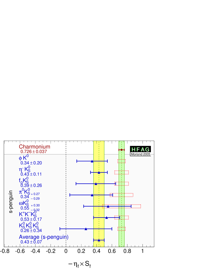
Figure 18: Averages for $S_{b\to q\overline{q}s}$ compared to $S_{b\to c\overline{c}s}$, with coarse dimensional estimates of associated theoretical uncertainties indicated by the open boxes.

5.7 Time-dependent $C\!P$ asymmetries in $b\to c\overline{c}d$ transitions

The transition $b\to c\overline{c}d$ can occur via either a $b\to c$ tree or a $b\to d$ penguin amplitude. Similarly to Eq. (98), the amplitude for the $b\to d$ penguin can be written

$$\begin{array}[]{ccccc}A_{b\to d}&=&\lx@intercol F_{u}V_{ub}V^{*}_{ud}+F_{c}V_{cb}V^{*}_{cd}+F_{t}V_{tb}V^{*}_{td}\hfil\lx@intercol\\ &=&(F_{u}-F_{c})V_{ub}V^{*}_{ud}&+&(F_{t}-F_{c})V_{tb}V^{*}_{td}\\ &=&{\cal O}(\lambda^{3})&+&{\cal O}(\lambda^{3}).\\ \end{array}$$ (99)

From this it can be seen that the $b\to d$ penguin amplitude does not have a dominant weak phase.

In the above, we have followed Eq. (98) by eliminating the $F_{c}$ term using unitarity. However, we could equally well write

$$\begin{array}[]{ccccc}A_{b\to d}&=&(F_{u}-F_{t})V_{ub}V^{*}_{ud}&+&(F_{c}-F_{t})V_{cb}V^{*}_{cd},\\ &=&(F_{c}-F_{u})V_{cb}V^{*}_{cd}&+&(F_{t}-F_{u})V_{tb}V^{*}_{td}.\\ \end{array}$$ (100)

Since the $b\to c\overline{c}d$ tree amplitude has the weak phase of $V_{cb}V^{*}_{cd}$, either of the above expressions allow the penguin to be decomposed into parts with weak phases the same and different to the tree amplitude (the relative weak phase can be chosen to be either $\beta$ or $\gamma$). However, if the tree amplitude dominates, there is little sensitivity to any phase other than that from $B^{0}$-$\kern 1.79993pt\overline{\kern-1.79993ptB}{}^{0}$ mixing.

The $b\to c\overline{c}d$ transitions can be investigated with studies of various different final states. Results are available from both BABAR  and Belle  using the final states ${J\mskip-3.0mu/\mskip-2.0mu\psi\mskip 2.0mu}\pi^{0}$, $D^{*+}D^{*-}$ and $D^{*\pm}D^{\mp}$; the averages of these results are given in Table 31. The results using the $C\!P$ eigenstate (${\eta}=+1$) ${J\mskip-3.0mu/\mskip-2.0mu\psi\mskip 2.0mu}\pi^{0}$ are shown in Fig. 19. The vector-vector mode $D^{*+}D^{*-}$ is found to be dominated by the $C\!P$ even longitudinally polarized component; BABAR measures a $C\!P$ odd fraction of $0.124\pm 0.044\pm 0.007$ [198] while Belle measures a $C\!P$ odd fraction of $0.19\pm 0.08\pm 0.01$ [199] (here we do not average these fractions and rescale the inputs, however the average is almost independent of the treatment). We treat the uncertainty due to the error in the $C\!P$-odd fractions (quoted as a third uncertainty) as a correlated systematic error. For the non-$C\!P$ eigenstate mode $D^{*\pm}D^{\mp}$ BABAR uses fully reconstructed events while Belle combines both fully and partially reconstructed samples.

Table 31: Averages for $b\to c\overline{c}d$ modes.

Experiment		$S_{b\to c\overline{c}d}$	$C_{b\to c\overline{c}d}$
${J\mskip-3.0mu/\mskip-2.0mu\psi\mskip 2.0mu}\pi^{0}$
BABAR	[196]	$\phantom{-}0.05\pm 0.49\pm 0.16$	$0.38\pm 0.41\pm 0.09$
Belle	[197]	$-0.72\pm 0.42\pm 0.09$	$0.01\pm 0.29\pm 0.03$
Average		$-0.40\pm 0.33$	$0.12\pm 0.24$
Confidence level		combined average: $0.36$
$D^{*+}D^{*-}$
BABAR	[198]	$-0.65\pm 0.26\pm 0.04^{+0.09}_{-0.07}$	$0.04\pm 0.14\pm 0.02$
Belle	[199]	$-0.75\pm 0.56\pm 0.10\pm 0.06$	$0.26\pm 0.26\pm 0.05\pm 0.01$
Average		$-0.67\pm 0.25$	$0.09\pm 0.12$
Confidence level		$0.89$	$0.47$

Experiment		$S_{+-}$	$C_{+-}$	$S_{-+}$	$C_{-+}$	$A$
$D^{*\pm}D^{\mp}$
BABAR	[200]	$-0.82\pm 0.75\pm 0.14$	$-0.47\pm 0.40\pm 0.12$	$-0.24\pm 0.69\pm 0.12$	$-0.22\pm 0.37\pm 0.10$	$-0.03\pm 0.11\pm 0.05$
Belle	[201]	$-0.55\pm 0.39\pm 0.12$	$-0.37\pm 0.22\pm 0.06$	$-0.96\pm 0.43\pm 0.12$	$\phantom{-}0.23\pm 0.25\pm 0.06$	$\phantom{-}0.07\pm 0.08\pm 0.04$
Average		$-0.61\pm 0.36$	$-0.39\pm 0.20$	$-0.75\pm 0.38$	$0.09\pm 0.21$	$0.03\pm 0.07$

In the absence of the penguin contribution, the time-dependent parameters would be given by $S_{b\to c\overline{c}d}=-{\eta}\sin(2\beta)$, $C_{b\to c\overline{c}d}=0$, $S_{+-}=\sin(2\beta+\delta)$, $S_{-+}=\sin(2\beta-\delta)$, $C_{+-}=-C_{-+}$ and $A_{+-}=0$, where $\delta$ is the strong phase difference between the $D^{*+}D^{-}$ and $D^{*-}D^{+}$ decay amplitudes. In the presence of the penguin contribution, there is no clean interpretation in terms of CKM parameters, however direct $C\!P$ violation may be observed as any of $C_{b\to c\overline{c}d}\neq 0$, $C_{+-}\neq-C_{-+}$ or $A_{+-}\neq 0$.

The averages for the $b\to c\overline{c}d$ modes are shown in Fig. 20. Comparisons of the results for the $b\to c\overline{c}d$ modes to the $b\to c\overline{c}s$ and $b\to q\overline{q}s$ modes, can be seen in Fig. 21.

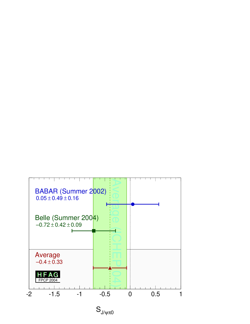
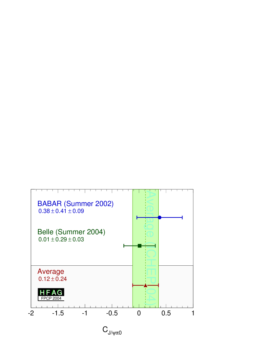
Figure 19: Averages of (left) $S_{b\to c\overline{c}d}$ and (right) $C_{b\to c\overline{c}d}$ for the mode $B^{0}\to J/\psi\pi^{0}$.

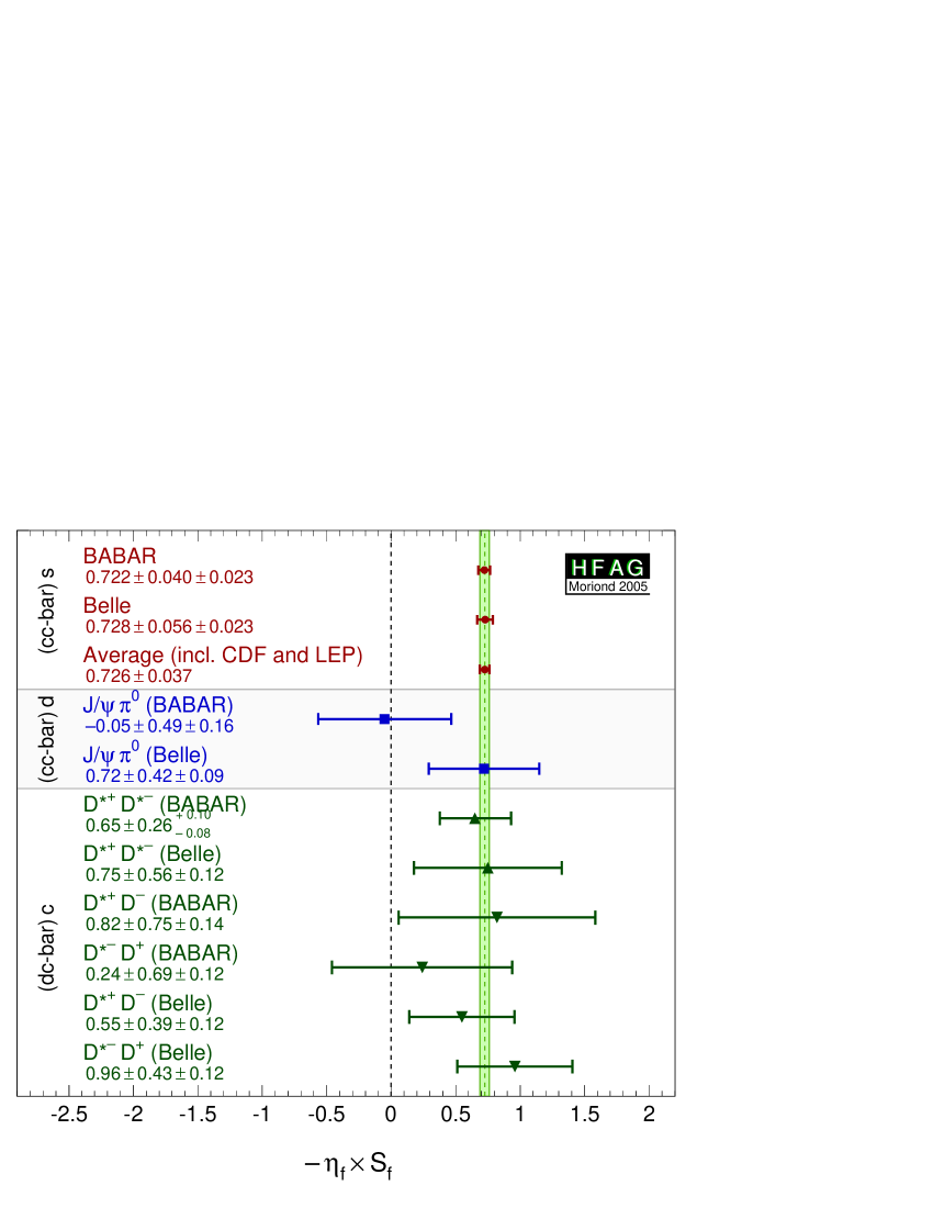
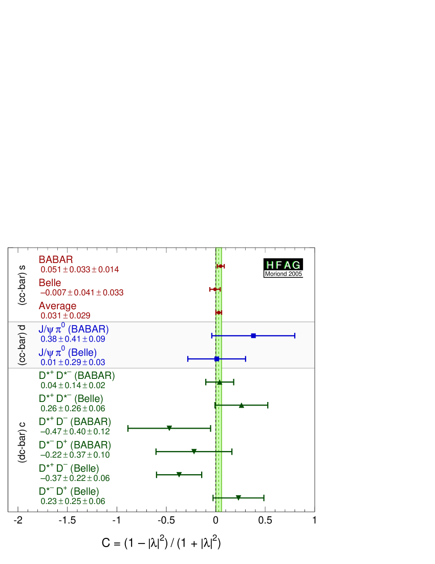
Figure 20: Averages of (left) $S_{b\to c\overline{c}d}$ and (right) $C_{b\to c\overline{c}d}$, compared to $S_{b\to c\overline{c}s}$ and $C_{b\to c\overline{c}s}$, respectively.

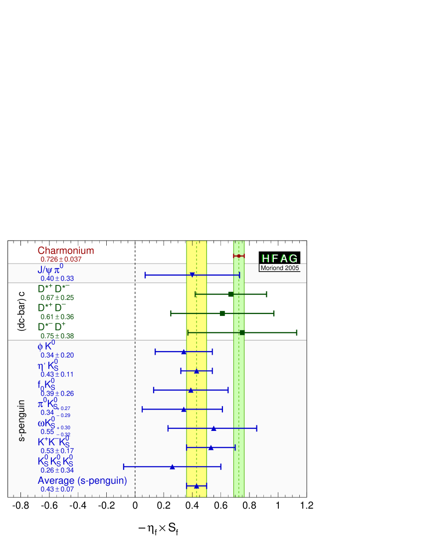
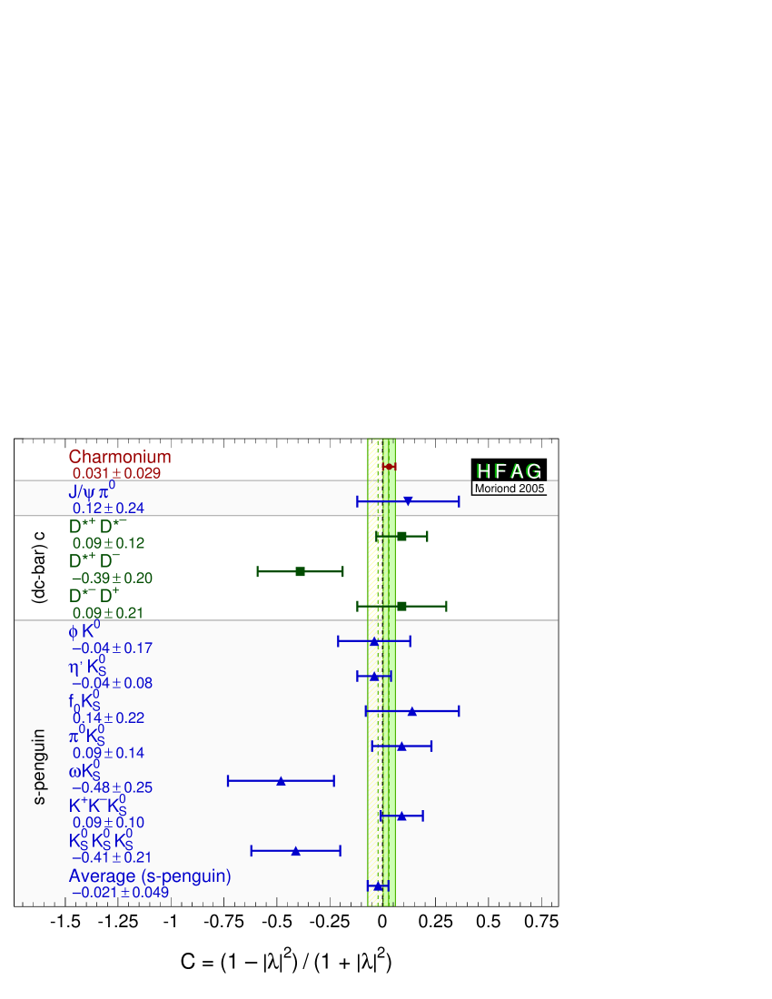
Figure 21: Comparisons of the averages of (left) $S_{b\to c\overline{c}s}$, $S_{b\to c\overline{c}d}$ and $S_{b\to q\overline{q}s}$, and (right) $C_{b\to c\overline{c}s}$, $C_{b\to c\overline{c}d}$ and $C_{b\to q\overline{q}s}$.

5.8 Time-dependent asymmetries in $b\to s\gamma$ transitions

The radiative decays $b\to s\gamma$ produce photons which are highly polarized in the Standard Model. The decays $B^{0}\to F\gamma$ and $\kern 1.79993pt\overline{\kern-1.79993ptB}{}^{0}\to F\gamma$ produce photons with opposite helicities, and since the polarization is, in principle, observable, these final states cannot interfere. The finite mass of the $s$ quark introduces small corrections to the limit of maximum polarization, but any large mixing induced $C\!P$ violation would be a signal for new physics. Since a single weak phase dominates the $b\to s\gamma$ transition in the Standard Model, the cosine term is also expected to be small.

Atwood et al. [171] have shown that an inclusive analysis with respect to $K^{0}_{\scriptscriptstyle S}\pi^{0}\gamma$ can be performed, since the properties of the decay amplitudes are independent of the angular momentum of the $K^{0}_{\scriptscriptstyle S}\pi^{0}$ system. However, if non-dipole operators contribute significantly to the amplitudes, then the Standard Model mixing-induced $C\!P$ violation could be larger than the naive expectation $S~{}-2(m_{s}/m_{b})\sin\left(2\beta\right)$, and the $C\!P$ parameters may vary over the $K^{0}_{\scriptscriptstyle S}\pi^{0}\gamma$ Dalitz plot, for example as a function of the $K^{0}_{\scriptscriptstyle S}\pi^{0}$ invariant mass.

With the above in mind, we quote two averages: one for $K^{*}(892)$ candidates only, and the other one for the inclusive $K^{0}_{\scriptscriptstyle S}\pi^{0}\gamma$ decay (including the $K^{*}(892)$). If the Standard Model dipole operator is dominant, both should give the same quantities (the latter naturally with smaller statistical error). If not, care needs to be taken in interpretation of the inclusive parameters, while the results on the $K^{*}(892)$ resonance remain relatively clean. Results from BABAR and Belle are used for both averages; both experiments use the invariant mass range $0.60\ {\rm GeV}/c^{2}<M_{K^{0}_{\scriptscriptstyle S}\pi^{0}}<1.80\ {\rm GeV}/c^{2}$ in the inclusive analysis.

Table 32: Averages for $b\to s\gamma$ modes.

Experiment		$S_{b\to s\gamma}$	$C_{b\to s\gamma}$
$K^{*}(892)\gamma$
BABAR	[202]	$-0.21\pm 0.40\pm 0.05$	$-0.40\pm 0.23\pm 0.04$
Belle	[203]	$-0.79\,^{+0.63}_{-0.50}\pm 0.10$	$0.00\,^{+0.37}_{-0.38}\pm 0.11$
Average		$-0.38\pm 0.34$	$-0.30\pm 0.20$
Confidence level		combined average: $0.50$
$K^{0}_{\scriptscriptstyle S}\pi^{0}\gamma$ (including $K^{*}(892)\gamma$)
BABAR	[202]	$-0.06\pm 0.37$	$-0.48\pm 0.22$
Belle	[203]	$-0.58\,^{+0.46}_{-0.38}\pm 0.11$	$-0.03\pm 0.34\pm 0.11$
Average		$-0.26\pm 0.29$	$-0.36\pm 0.19$
Confidence level		combined average: $0.38$

5.9 Time-dependent $C\!P$ asymmetries in $b\to u\overline{u}d$ transitions

The $b\to u\overline{u}d$ transition can be mediated by either a $b\to u$ tree amplitude or a $b\to d$ penguin amplitude. These transitions can be investigated using the time dependence of $B^{0}$ decays to final states containing light mesons. Results are available from both BABAR and Belle for the $C\!P$ eigenstate (${\eta}=+1$) $\pi^{+}\pi^{-}$ final state. BABAR  has also performed an analysis on the vector-vector final state $\rho^{+}\rho^{-}$, which they find to be dominated by the $C\!P$ even longitudinally polarized component (they measure $f_{\rm long}=0.978\pm 0.014\,^{+0.021}_{-0.029}$ [208]).

For the non-$C\!P$ eigenstate $\rho^{\pm}\pi^{\mp}$, Belle has performed a quasi-two-body analysis, while BABAR performs a time-dependent Dalitz plot (DP) analysis of the $\pi^{+}\pi^{-}\pi^{0}$ final state [205]; such an analysis allows direct measurements of the phases. These results, and averages, are listed in Table 33. The averages for $\pi^{+}\pi^{-}$ are shown in Fig. 22.

Table 33: Averages for $b\to u\overline{u}d$ modes.

Experiment		$S_{b\to u\overline{u}d}$	$C_{b\to u\overline{u}d}$
	$\pi^{+}\pi^{-}$
BABAR	[206]	$-0.30\pm 0.17\pm 0.03$	$-0.09\pm 0.15\pm 0.04$
Belle	[207]	$-0.67\pm 0.16\pm 0.06$	$-0.56\pm 0.12\pm 0.06$
Average		$-0.50\pm 0.12$	$-0.37\pm 0.10$
Confidence level		combined average: $0.019~{}(2.3\sigma)$
	$\rho^{+}\rho^{-}$
BABAR	[208]	$-0.33\pm 0.24\,^{+0.08}_{-0.14}$	$-0.03\pm 0.18\pm 0.09$

	$\rho^{\pm}\pi^{\mp}$ Q2B/DP analysis
Experiment		$S_{\rho\pi}$	$C_{\rho\pi}$	$\Delta S_{\rho\pi}$	$\Delta C_{\rho\pi}$	${\cal A}_{CP}^{\rho\pi}$
BABAR	[211]	$-0.10\pm 0.14\pm 0.04$	$0.34\pm 0.11\pm 0.05$	$\phantom{-}0.22\pm 0.15\pm 0.03$	$0.15\pm 0.11\pm 0.03$	$-0.088\pm 0.049\pm 0.013$
Belle	[210]	$-0.28\pm 0.23\,^{+0.10}_{-0.08}$	$0.25\pm 0.17\,^{+0.02}_{-0.06}$	$-0.30\pm 0.24\pm 0.09$	$0.38\pm 0.18\,^{+0.02}_{-0.04}$	$-0.16\pm 0.10\pm 0.02$
Average		$-0.13\pm 0.13$	$0.31\pm 0.10$	$0.09\pm 0.13$	$0.22\pm 0.10$	$-0.102\pm 0.045$
			${\cal A}^{+-}_{\rho\pi}$		${\cal A}^{-+}_{\rho\pi}$
BABAR	[211]		$\phantom{-}0.25\pm 0.17\,^{+0.02}_{-0.06}$		$-0.47^{\,+0.14}_{\,-0.15}\pm 0.06$
Belle	[210]		$-0.02\pm 0.16^{\,+0.05}_{\,-0.02}$		$-0.53\pm 0.29^{\,+0.09}_{\,-0.04}$
Average			$-0.15\pm 0.09$		$-0.47^{\,+0.13}_{\,-0.14}$

$\rho^{\pm}\pi^{\mp}$ DP analysis
Experiment		$\alpha\ (^{\circ})$	$\delta_{+-}\ (^{\circ})$
BABAR	[211]	$113\,^{+27}_{-17}\pm 6$	$-67\,^{+28}_{-31}\pm 7$

If the penguin contribution is negligible, the time-dependent parameters for $B^{0}\to\pi^{+}\pi^{-}$ and $B^{0}\to\rho^{+}\rho^{-}$ are given by $S_{b\to u\overline{u}d}={\eta}\sin(2\alpha)$ and $C_{b\to u\overline{u}d}=0$. With the notation described in Sec. 5.2 (Eq. (85)), the time-dependent parameters for $B^{0}\to\rho^{\pm}\pi^{\mp}$ are, neglecting penguin contributions, given by $S_{\rho\pi}=\sqrt{1-(\frac{\Delta C}{2})^{2}}\sin(2\alpha)\cos(\delta)$, $\Delta S_{\rho\pi}=\sqrt{1-(\frac{\Delta C}{2})^{2}}\cos(2\alpha)\sin(\delta)$ and $C_{\rho\pi}={\cal A}_{C\!P}^{\rho\pi}=0$, where $\delta=\arg(A_{-+}A^{*}_{+-})$ is the strong phase difference between the $\rho^{-}\pi^{+}$ and $\rho^{+}\pi^{-}$ decay amplitudes. In the presence of the penguin contribution, there is no straightforward interpretation of $B^{0}\to\rho^{\pm}\pi^{\mp}$ in terms of CKM parameters. However direct $C\!P$ violation may arise, resulting in either or both of $C_{\rho\pi}\neq 0$ and ${\cal A}_{C\!P}^{\rho\pi}\neq 0$. Equivalently, direct $C\!P$ violation may be seen by either of the decay-type-specific observables ${\cal A}^{+-}_{\rho\pi}$ and ${\cal A}^{-+}_{\rho\pi}$, defined in Eq. (86), deviating from zero. Results and averages for these parameters are also given in Table 33. They exhibit a linear correlation coefficient of $+0.59$. The significance of observing direct $C\!P$ violation computed from the difference of the $\chi^{2}$ obtained in the nominal average, compared to setting $C_{\rho\pi}={\cal A}^{\rho\pi}_{C\!P}=0$ is found to be $3.4\sigma$ in this mode. The confidence level contours of ${\cal A}^{+-}_{\rho\pi}$ versus ${\cal A}^{-+}_{\rho\pi}$ are shown in Fig. 23.

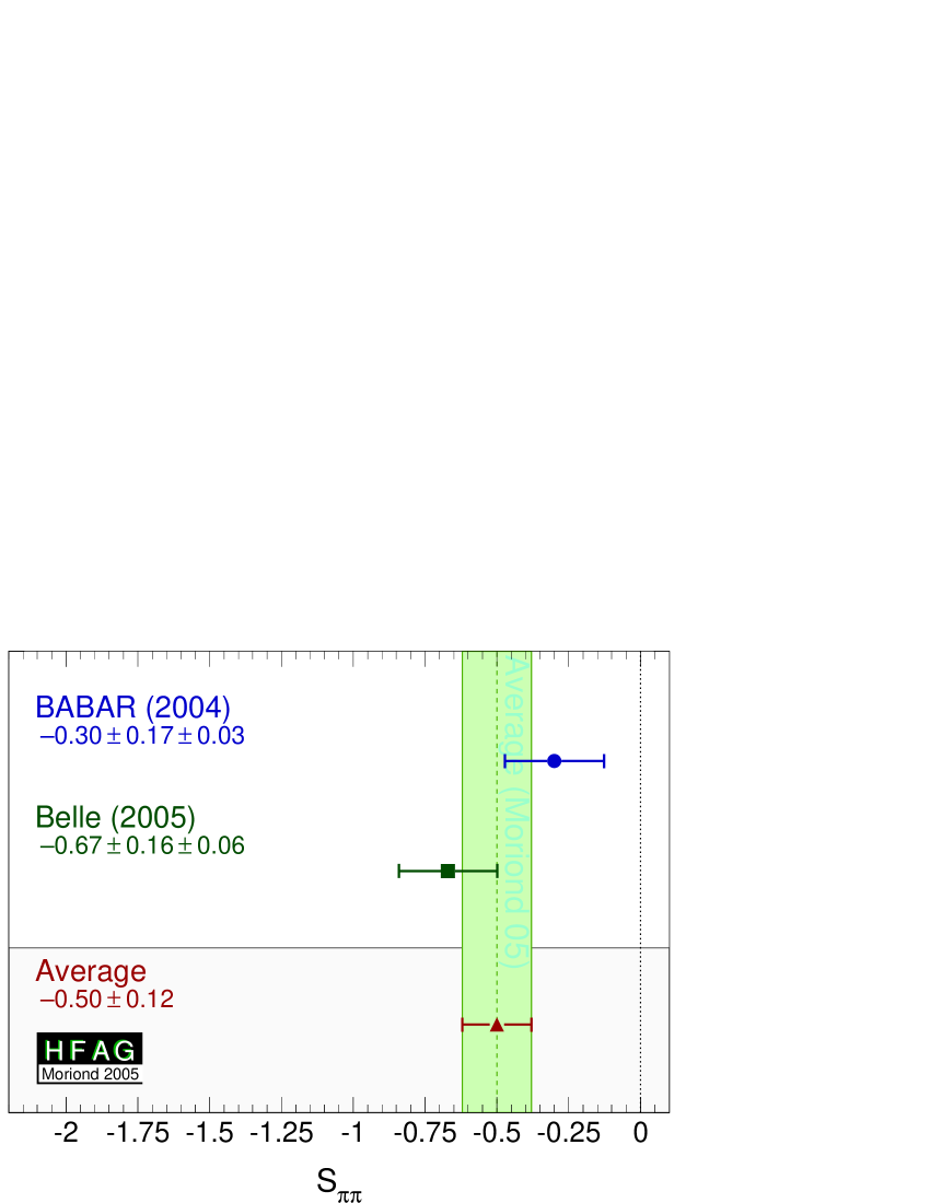
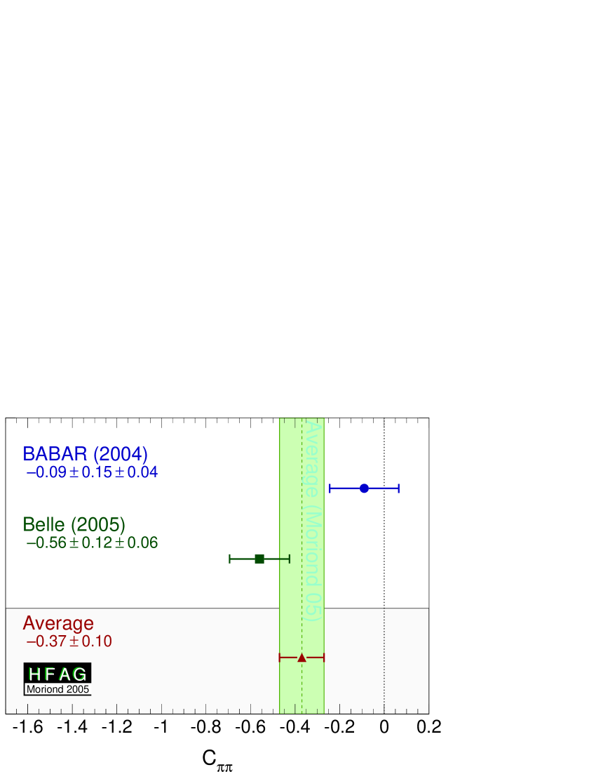
Figure 22: Averages of (left) $S_{b\to u\overline{u}d}$ and (right) $C_{b\to u\overline{u}d}$ for the mode $B^{0}\to\pi^{+}\pi^{-}$.

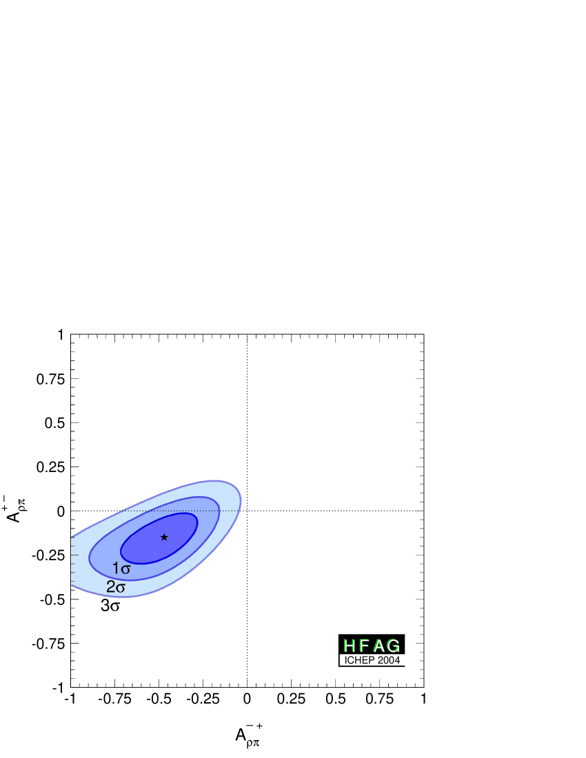
Figure 23: Direct $C\!P$ violation in $B^{0}\to\rho^{\pm}\pi^{\mp}$. The no-$C\!P$ violation hypothesis is excluded at the $3.4\sigma$ level.

Some difference is seen between the BABAR and Belle measurements in the $\pi^{+}\pi^{-}$ system. The confidence level of the average is $0.019$, which corresponds to a $2.3\sigma$ discrepancy. Since there is no evidence of systematic problems in either analysis, we do not rescale the errors of the averages.

The precision of the measured $C\!P$ violation parameters in $b\to u\overline{u}d$ transitions allows constraints to be set on the UT angle $\alpha$. In addition to the value of $\alpha$ from the BABAR time-dependent DP analysis, given in Table 33, constraints have been obtained with various methods:

• Both BABAR [206] and Belle [207] have performed isospin analyses in the $\pi^{+}\pi^{-}$ system. BABAR exclude $29^{\circ}<\alpha<61^{\circ}$ at the $90\%$ C.L. while Belle exclude $19^{\circ}<\alpha<71^{\circ}$ at the $95.4\%$ C.L. In both cases, only solutions in $0^{\circ}$—$180^{\circ}$ are considered.

• Using the measured time-dependent $C\!P$ violation parameters in longitudinally polarized $B^{0}\to\rho^{+}\rho^{-}$ decays [208], in combination with the upper limit for the $B^{0}\to\rho^{0}\rho^{0}$ branching fraction [213], and the measurement of the branching fraction and longitudinal polarization of $B^{+}\to\rho^{+}\rho^{0}$ [214, 215], BABAR performs an isospin analysis [216] and obtains $\alpha=(100\pm 13)^{\circ}$, using the solution closest to the CKM combined fit average. The $90\%$ C.L. allowed region for that solution is $79^{\circ}<\alpha<123^{\circ}$.

• The CKMfitter group [183] uses the measurements from Belle and BABAR given in Table 33, with other branching fractions and $C\!P$ asymmetries in $B\to\pi\pi,~{}\rho\pi$ and $\rho\rho$ modes, to perform isospin analyses for each system. They then combine the results to obtain $\alpha=(97.9\,^{+5.0}_{-6.4})^{\circ}$. Similarly, the UTFit group [184] obtain $\alpha=(94.9\pm 6.6)^{\circ}$.

Note that each method suffers from ambiguities in the solutions. All the above measurements correspond to the choice that is in agreement with the global CKM fit.

At present we make no attempt to provide an HFAG average for $\alpha$. More details on procedures to calculate a best fit value for $\alpha$ can be found in Refs. [183, 184].

5.10 Time-dependent $C\!P$ asymmetries in $b\to c\overline{u}d/u\overline{c}d$ transitions

Non-$C\!P$ eigenstates such as $D^{\pm}\pi^{\mp}$, $D^{*\pm}\pi^{\mp}$ and $D^{\pm}\rho^{\mp}$ can be produced in decays of $B^{0}$ mesons either via Cabibbo favoured ($b\to c$) or doubly Cabibbo suppressed ($b\to u$) tree amplitudes. Since no penguin contribution is possible, these modes are theoretically clean. The ratio of the magnitudes of the suppressed and favoured amplitudes, $R$, is sufficiently small (predicted to be about $0.02$), that terms of ${\cal O}(R^{2})$ can be neglected, and the sine terms give sensitivity to the combination of UT angles $2\beta+\gamma$.

As described in Sec. 5.2.4, the averages are given in terms of parameters $a$ and $c$. $C\!P$ violation would appear as $a\neq 0$. Results are available from both BABAR and Belle in the modes $D^{\pm}\pi^{\mp}$ and $D^{*\pm}\pi^{\mp}$; for the latter mode both experiments have used both full and partial reconstruction techniques. Results are also available from BABAR using $D^{\pm}\rho^{\mp}$. These results, and their averages, are listed in Table 34, and are shown in Fig. 24.

Table 34: Averages for $b\to c\overline{u}d/u\overline{c}d$ modes.

Experiment		$a$	$c$
$D^{*\pm}\pi^{\mp}$
BABAR (full rec.)	[217]	$-0.049\pm 0.031\pm 0.020$	$\phantom{-}0.044\pm 0.054\pm 0.033$
Belle (full rec.)	[218]	$\phantom{-}0.060\pm 0.040\pm 0.019$	$\phantom{-}0.049\pm 0.040\pm 0.019$
BABAR (partial rec.)	[219]	$-0.034\pm 0.014\pm 0.009$	$-0.019\pm 0.022\pm 0.013$
Belle (partial rec.)	[220]	$-0.030\pm 0.028\pm 0.018$	$-0.005\pm 0.028\pm 0.018$
Average		$-0.027\pm 0.013$	$0.001\pm 0.018$
Confidence level		$0.22$	$0.52$
$D^{\pm}\pi^{\mp}$
BABAR (full rec.)	[217]	$-0.032\pm 0.031\pm 0.020$	$-0.059\pm 0.055\pm 0.033$
Belle (full rec.)	[218]	$-0.062\pm 0.037\pm 0.018$	$-0.025\pm 0.037\pm 0.018$
Average		$-0.045\pm 0.027$	$-0.035\pm 0.035$
Confidence level		$0.59$	$0.66$
$D^{\pm}\rho^{\mp}$
BABAR (full rec.)	[217]	$-0.005\pm 0.044\pm 0.021$	$-0.147\pm 0.074\pm 0.035$

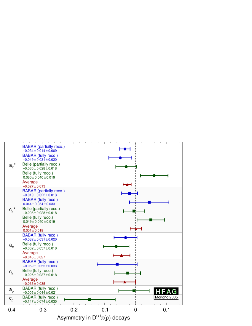
Figure 24: Averages for $b\to c\overline{u}d/u\overline{c}d$ modes.

5.11 Rates and asymmetries in $B^{\mp}\to D^{(*)}K^{(*)\mp}$ decays

As explained in Sec. 5.2.5, rates and asymmetries in $B^{\mp}\to D^{(*)}K^{(*)\mp}$ decays are sensitive to $\gamma$. Various methods using different $D^{(*)}$ final states exist.

Results are available from both BABAR and Belle on GLW analyses in the decay modes $B^{\mp}\to DK^{\mp}$, $B^{\mp}\to D^{*}K^{\mp}$ and $B^{\mp}\to DK^{*\mp}$. Both experiments use the $C\!P$ even $D$ decay final states $K^{+}K^{-}$ and $\pi^{+}\pi^{-}$ in all three modes; both experiments also use only the $D^{*}\to D\pi^{0}$ decay, which gives $C\!P(D^{*})=C\!P(D)$. For $C\!P$ odd $D$ decay final states, Belle uses $K^{0}_{\scriptscriptstyle S}\pi^{0}$, $K^{0}_{\scriptscriptstyle S}\eta$ and $K^{0}_{\scriptscriptstyle S}\phi$ in all three analyses, and also use $K^{0}_{\scriptscriptstyle S}\omega$ in $DK^{\mp}$ and $D^{*}K^{\mp}$ analyses. BABAR uses $K^{0}_{\scriptscriptstyle S}\pi^{0}$ only for $DK^{\mp}$ analysis; for $DK^{*\mp}$ analysis they also use $K^{0}_{\scriptscriptstyle S}\phi$ and $K^{0}_{\scriptscriptstyle S}\omega$ (and assign an asymmetric systematic error due to $C\!P$ even pollution in these $C\!P$ odd channels [225]). The results and averages are given in Table 35.

Table 35: Averages from GLW analyses of $b\to c\overline{u}d/u\overline{c}d$ modes.

Experiment		$A_{C\!P+}$	$A_{C\!P-}$	$R_{C\!P+}$	$R_{C\!P-}$
$D_{C\!P}K^{-}$
BABAR	[223]	$\phantom{-}0.40\pm 0.15\pm 0.08$	$\phantom{-}0.21\pm 0.17\pm 0.07$	$0.87\pm 0.14\pm 0.06$	$0.80\pm 0.14\pm 0.08$
Belle	[224]	$\phantom{-}0.07\pm 0.14\pm 0.06$	$-0.11\pm 0.14\pm 0.05$	$0.98\pm 0.18\pm 0.10$	$1.29\pm 0.16\pm 0.08$
Average		$0.22\pm 0.11$	$0.02\pm 0.12$	$0.91\pm 0.12$	$1.02\pm 0.12$
$D^{*}_{C\!P}K^{-}$
BABAR	[225]	$-0.10\pm 0.23\,^{+0.03}_{-0.04}$		$1.06\pm 0.26\,^{+0.10}_{-0.09}$
Belle	[224]	$-0.27\pm 0.25\pm 0.04$	$0.26\pm 0.26\pm 0.03$	$1.43\pm 0.28\pm 0.06$	$0.94\pm 0.28\pm 0.06$
Average		$-0.18\pm 0.17$	$0.26\pm 0.26$	$1.24\pm 0.20$	$0.94\pm 0.29$
$D_{C\!P}K^{*-}$
BABAR	[226]	$-0.09\pm 0.20\pm 0.06$	$-0.33\pm 0.34\pm 0.10\,^{+0.00}_{-0.06}$	$1.77\pm 0.37\pm 0.12$	$0.76\pm 0.29\pm 0.06\,^{+0.04}_{-0.14}$
Belle	[227]	$-0.02\pm 0.33\pm 0.07$	$0.19\pm 0.50\pm 0.04$
Average		$-0.07\pm 0.18$	$-0.16\pm 0.29$

For ADS analysis, both BABAR and Belle have studied the mode $B^{\mp}\to DK^{\mp}$; Belle has also studied $B^{\mp}\to\pi^{\mp}$ and BABAR has also analyzed the $B^{\mp}\to D^{*}K^{\mp}$ mode ($D^{*}\to D\pi^{0}$ and $D^{*}\to D\gamma$ are studied separately). In all cases the suppressed decay $D\to K^{+}\pi^{-}$ has been used. The results and averages are given in Table 36. Note that although no clear signals for these modes have yet been seen, the central values are given in Table 36. In $B^{-}\to D^{*}K^{-}$ decays there is an effective shift of $\pi$ in the strong phase difference between the cases that the $D^{*}$ is reconstructed as $D\pi^{0}$ and $D\gamma$ [176]. As a consequence, the different $D^{*}$ decay modes are treated separately.

Table 36: Averages from ADS analyses of $b\to c\overline{u}d/u\overline{c}d$ modes.

Experiment		$A_{ADS}$	$R_{ADS}$
$DK^{-}$, $D\to K^{+}\pi^{-}$
BABAR	[228]		$0.013\,^{+0.011}_{-0.009}$
Belle	[229]	$0.88\,^{+0.77}_{-0.62}\pm 0.06$	$0.023\,^{+0.016}_{-0.014}\pm 0.001$
Average		$0.88\,^{+0.77}_{-0.62}$	$0.017\pm 0.009$
$D^{*}K^{-}$, $D^{*}\to D\pi^{0}$, $D\to K^{+}\pi^{-}$
BABAR	[228]		$-0.001\,^{+0.010}_{-0.006}$
$D^{*}K^{-}$, $D^{*}\to D\gamma$, $D\to K^{+}\pi^{-}$
BABAR	[228]		$0.011\,^{+0.019}_{-0.013}$
$D\pi^{-}$, $D\to K^{+}\pi^{-}$
Belle	[229]	$0.30\,^{+0.29}_{-0.25}\pm 0.06$	$0.0035\,^{+0.0010}_{-0.0009}\pm 0.0002$

For the Dalitz plot analysis, both BABAR and Belle have studied the mode $B^{\mp}\to DK^{\mp}$. Both have also studied the mode $B^{\mp}\to D^{*}K^{\mp}$; Belle has used only $D^{*}\to D\pi^{0}$, while BABAR has used both $D^{*}$ decay modes and taken the effective shift in the strong phase difference into account. Belle has also released results using $B^{\mp}\to DK^{*\mp}$; in this case an additional uncertainty arises from other possible $B^{\mp}\to DK^{0}_{\scriptscriptstyle S}\pi^{\mp}$ contributions. In all cases the decay $D\to K^{0}_{\scriptscriptstyle S}\pi^{+}\pi^{-}$ has been used. The results are given in Table 37. Since the measured values of $r_{B}$ are positive definite, and since the error on $\gamma$ depends on the value of $r_{B}$, some statistical treatment is necessary to correct for bias. At present, both BABAR and Belle use frequentist treatments. At present, we make no attempt to average the results.

Table 37: Averages from Dalitz plot analyses of $b\to c\overline{u}d/u\overline{c}d$ modes.

Experiment		$\gamma\ (^{\circ})$	$\delta_{B}\ (^{\circ})$	$r_{B}$
$DK^{-}$, $D\to K^{0}_{\scriptscriptstyle S}\pi^{+}\pi^{-}$
BABAR	[230]		$104\pm 45\,+{+17}_{-21}\,^{+16}{}_{-24}$	$0.12\pm 0.08\pm 0.03\pm 0.04$
Belle	[231]	$64\pm 19\pm 13\pm 11$	$157\pm 19\pm 11\pm 21$	$0.21\pm 0.08\pm 0.03\pm 0.04$
Average		in preparation
$D^{*}K^{-}$, $D^{*}\to D\pi^{0}$ or $D\gamma$, $D\to K^{0}_{\scriptscriptstyle S}\pi^{+}\pi^{-}$
BABAR	[230]		$296\pm 41\,^{+14}_{-12}\pm 15$	$0.17\pm 0.10\pm 0.03\pm 0.03$
Belle	[231]	$75\pm 57\pm 11\pm 11$	$321\pm 57\pm 11\pm 21$	$0.12\,^{+0.16}_{-0.11}\pm 0.02\pm 0.04$
Average		in preparation
$DK^{-}$ and $D^{*}K^{-}$ combined
BABAR	[230]	$70\pm 31\,^{+12}_{-10}\,{}^{+14}_{-11}$
Belle	[231]	$68\,^{+14}_{-15}\pm 13\pm 11$
Average		in preparation
$DK^{*-}$, $D\to K^{0}_{\scriptscriptstyle S}\pi^{+}\pi^{-}$
Belle	[232]	$112\pm 35\pm 9\pm 11\pm 8$	$353\pm 35\pm 8\pm 21\pm 49$	$0.25\pm 0.18\pm 0.09\pm 0.04\pm 0.08$

6 Charmless $B$-decay branching fractions and their asymmetries

The aim of this section is to provide the branching fractions and the partial rate asymmetries ($A_{CP}$) of rare $B$ decays. The asymmetry is defined as $A_{CP}=\frac{N_{\kern 0.89996pt\overline{\kern-0.89996ptB}{}}-N_{B}}{N_{\kern 0.89996pt\overline{\kern-0.89996ptB}{}}+N_{B}}$, where $N_{\kern 1.25995pt\overline{\kern-1.25995ptB}{}}$ and $N_{B}$ are number of $\kern 1.79993pt\overline{\kern-1.79993ptB}{}^{0}/B^{-}$ and $B^{0}/B^{+}$, respectively. Four different $B$ decay categories are considered: charmless mesonic, baryonic, radiative and leptonic. Rare mesonic decays with charm are not in our scope but results of charmful baryonic decays are included. Measurements supported with written documents are accepted in our the averages; written documents could be journal papers, conference contributed papers, preprints or conference proceedings. Results from $A_{CP}$ measurements obtained from time dependent analyses are listed and described in Sec. 5.

So far all branching fractions assume equal production of charged and neutral $B$ pairs. The best measurements to date show that this is still a good approximation (see Sec. 3.1.1). For branching fractions, we provide either averages or the most stringent 90% confidence level upper limits. If one or more experiments have measurements with $>$4$\sigma$ for a decay channel, all available central values for that channel are used in the averaging. We also give central values and errors for cases where the significance of the average value is at least $3\sigma$, even if no single measurement is above $4\sigma$. For $A_{CP}$ we provide averages in all cases.

Our averaging is performed by maximizing the likelihood,

$${\mathcal{L}}=\prod_{i}{\mathcal{P}}_{i}(x),$$ (101)

where ${\mathcal{P}_{i}}$ is the probability density function (PDF) of the $i$th measurement, and $x$ is the branching fraction or $A_{CP}$. The PDF is modeled by an asymmetric Gaussian function with the measured central value as its mean and the quadratic sum of the statistical and systematic errors as the standard deviations. The experimental uncertainties are considered to be uncorrelated with each other when the averaging is performed. No error scaling is applied when the fit $\chi^{2}$ is greater than 1 since we believe that tends to overestimate the errors except in cases of extreme disagreement (we have no such cases).

At present, we have measurements of 236 $B$ decay modes including 4 $B_{s}$ decays newly added in this update cycle and asymmetry measurements for 43 of these decays. The averages of polarization measurements for $B\to$ charmless vector meson are also added in this update cycle. These results are reported in about 150 separate papers. Because the number of references is so large, we do not include them with the tables shown here but the full set of references is available quickly from active gifs at the “Winter 2005” link on the rare web page: http://www.slac.stanford.edu/xorg/hfag/rare/index.html

6.1 Mesonic charmless decays

Table 38: $B^{+}$ branching fractions (in units of $10^{-6}$). Upper limits are at 90% CL. Values in red (blue) are new published (preliminary) result since PDG2004 [as of April 2, 2005].

RPP#	Mode	PDG2004 Avg.	BABAR	Belle	CLEO	CDF	New Avg.
117	$K^{0}\pi^{+}$	$18.8\pm 2.1$	${{26.0}\pm{1.3}\pm{1.0}}$	${{22.0}\pm{1.9}\pm{1.1}}$	${{18.8}^{+3.7+2.1}_{-3.3-1.8}}$		$24.1\pm 1.3$
118	$K^{+}\pi^{0}$	$12.9\pm 1.2$	${{12.0}\pm{0.7}\pm{0.6}}$	${{12.0}\pm 1.3^{+1.3}_{-0.9}}$	${{12.9}^{+2.4+1.2}_{-2.2-1.1}}$		$12.1\pm 0.8$
119	${\eta^{\prime}}K^{+}$	$78\pm 5$	${{68.9}\pm{2.0}\pm{3.2}}$	${{78}\pm{6}\pm{9}}$	${{80}^{+10}_{-9}\pm 7}$		$70.8\pm 3.4$
120	${\eta^{\prime}}K^{*+}$	$<35$	$<14$	$<90$	$<35$		$<14$
121	$\eta K^{+}$	$<6.9$	${{3.3}\pm{0.6}\pm{0.3}}$	${{2.1}\pm{0.6}\pm{0.2}}$	${{2.2}^{+2.8}_{-2.2}}$		$2.6\pm 0.5$
122	$\eta K^{*+}$	${{26}^{+10}_{-9}}$	${{25.6}\pm{4.0}\pm{2.4}}$	${{22.8}^{+3.7}_{-3.5}\pm 2.2}$	${{26.4}^{+9.6}_{-8.2}\pm 3.3}$		${{24.3}^{+3.0}_{-2.9}}$
$~{}-$	$a_{0}^{0}(980)K^{+}$ ${\dagger}$	New	$<2.5$				$<2.5$
$~{}-$	$a_{0}^{+}(980)K^{0}$ ${\dagger}$	New	$<3.9$				$<3.9$
123	$\omega K^{+}$	${{9.2}^{+2.8}_{-2.5}}$	${{4.8}\pm{0.8}\pm{0.4}}$	${{6.5}^{+1.3}_{-1.2}\pm 0.6}$	${{3.2}^{+2.4}_{-1.9}\pm 0.8}$		$5.1\pm 0.7$
124	$\omega K^{*+}$	$<87$	$<7.4$		$<87$		$<7.4$
125	$K^{*0}\pi^{+}$	${{19}^{+6}_{-8}}$	${{10.5}\pm{1.9}\pm{1.6}}$	${{9.8}\pm 0.9^{+1.1}_{-1.2}}$	${{7.6}^{+3.5}_{-3.0}\pm 1.6}$		$9.7\pm 1.2$
126	$K^{*+}\pi^{0}$	$<31$	${{6.9}\pm{2.0}\pm{1.3}}$		${{7.1}^{+11.4}_{-7.1}\pm 1.0}$		$6.9\pm 2.3$
127	$K^{+}\pi^{+}\pi^{-}$	$57\pm 4$	${{61.4}\pm{2.4}\pm{4.5}}$	${{46.6}\pm{2.1}\pm{4.3}}$			$53.5\pm 3.5$
128	$K^{+}\pi^{+}\pi^{-}(NR)$	$<28$	${{4.9}\pm{0.6}\pm{1.4}}$		$<28$		$4.9\pm 1.5$
129	$K^{+}f_{0}(980)$ ${\dagger}$	seen	${{9.2}\pm{1.5}\pm{1.0}}$	${{7.6}\pm 1.2^{+1.6}_{-1.2}}$			${{8.4}^{+1.4}_{-1.3}}$
130	$K^{+}\rho^{0}$	$<12$	${{5.2}\pm{1.2}\pm{0.8}}$	${{4.78}\pm 0.75^{+1.01}_{-0.97}}$	${{8.4}^{+4.0}_{-3.4}\pm 1.8}$		${{5.15}^{+0.93}_{-0.91}}$
$~{}-$	$f_{2}(1270)K^{+}$ ${\dagger}$	New		$<1.3$			$<1.3$
$~{}-$	$f_{2}^{\prime}(1525)K^{+}$ ${\dagger}$	New		$<4.9$			$<4.9$
$~{}-$	$K^{*}_{0}(1430)^{0}\pi^{+}$ †	New	${{32.3}\pm{1.9}\pm{3.4}}$	$\mbox{${{45.0}^{+2.9}_{-15.0}\pm 10.7}$}{\ddagger}$			${{32.9}^{+3.7}_{-3.9}}$
131	$K^{*}_{2}(1430)^{0}\pi^{+}$${\dagger}$	$<680$		$<2.3$			$<2.3$
$~{}-$	$K^{*}(1680)^{0}\pi^{+}$ ${\dagger}$	New		$<3.1$			$<3.1$
132	$K^{-}\pi^{+}\pi^{+}$	$<1.8$	$<1.8$	$<4.5$			$<1.8$
135	$K^{0}\pi^{+}\pi^{0}$	$<66$			$<66$		$<66$
136	$K^{0}\rho^{+}$	$<48$			$<48$		$<48$
$~{}-$	$K^{*0}\rho^{+}$	New	${{17.0}\pm 2.9^{+2.0}_{-2.8}}$	${{8.9}\pm{1.7}\pm{1.0}}$			$10.5\pm 1.8$
138	$K^{*+}\rho^{0}$	$11\pm 4$	${{10.6}^{+3.0}_{-2.6}\pm 2.4}$		$<74$		${{10.6}^{+3.8}_{-3.5}}$
139	$K^{*+}\overline{K^{*0}}$	$<71$			$<71$		$<71$
142	$K^{+}\overline{K^{0}}$	$<2.0$	$<2.4$	$<3.3$	$<3.3$		$<2.4$
143	$K^{+}\overline{K^{0}}\pi^{0}$	$<24$			$<24$		$<24$
144	$K^{+}K_{S}K_{S}$	$13.4\pm 2.4$	${{10.7}\pm{1.2}\pm{1.0}}$	${{13.4}\pm{1.9}\pm{1.5}}$			$11.5\pm 1.3$
145	$K_{S}K_{S}\pi^{+}$	$<3.2$		$<3.2$			$<3.2$
146	$K^{+}K^{-}\pi^{+}$	$<6.3$	$<6.3$	$<13$			$<6.3$
148	$K^{+}K^{+}\pi^{-}$	$<1.3$	$<1.3$	$<2.4$			$<1.3$
150	$\overline{K^{*0}}K^{+}$	$<5.3$			$<5.3$		$<5.3$
152	$K^{+}K^{-}K^{+}$	$30.8\pm 2.1$	${{29.6}\pm{2.1}\pm{1.6}}$	${{30.6}\pm{1.2}\pm{2.3}}$			$30.1\pm 1.9$
153	$\phi K^{+}$	$9.3\pm 1.0$	${{10.0}^{+0.9}_{-0.8}\pm 0.5}$	${{9.60}\pm 0.92^{+1.05}_{-0.84}}$	${{5.5}^{+2.1}_{-1.8}\pm 0.6}$	${{7.6}\pm{1.3}\pm{0.6}}$	${{9.03}^{+0.65}_{-0.63}}$
$~{}-$	$a_{2}K^{+}$†	New		$<1.1$			$<1.1$
$~{}-$	$\phi(1680)K^{+}$†	New		$<0.8$			$<0.8$
156	$\phi K^{*+}$	$9.6\pm 3.0$	${{12.7}^{+2.2}_{-2.0}\pm 1.1}$	${{6.7}^{+2.1+0.7}_{-1.9-1.0}}$	${{10.6}^{+6.4+1.8}_{-4.9-1.6}}$		$9.7\pm 1.5$
159	$\phi\phi K^{+}$ §	${{2.6}^{+1.1}_{-0.9}}$		${{2.6}^{+1.1}_{-0.9}\pm 0.3}$			${{2.6}^{+1.1}_{-0.9}}$
173	$\pi^{+}\pi^{0}$	${{5.6}^{+0.9}_{-1.1}}$	${{5.8}\pm{0.6}\pm{0.4}}$	${{5.0}\pm{1.2}\pm{0.5}}$	${{4.6}^{+1.8+0.6}_{-1.6-0.7}}$		$5.5\pm 0.6$
174	$\pi^{+}\pi^{-}\pi^{+}$	$11\pm 4$	${{16.2}\pm{2.1}\pm{1.3}}$				$16.2\pm 2.5$
175	$\rho^{0}\pi^{+}$	$8.6\pm 2.0$	${{9.4}\pm{1.3}\pm{1.2}}$	${{8.0}^{+2.3}_{-2.0}\pm 0.7}$	${{10.4}^{+3.3}_{-3.4}\pm 2.1}$		${{9.1}^{+1.4}_{-1.3}}$
$~{}-$	$\rho^{0}(1450)\pi^{+}$	New	${{2.2}\pm{0.5}\pm{0.4}}$				$2.2\pm 0.6$
176	$\pi^{+}f_{0}(980)$ ${\dagger}$	$<140$					$<140$
177	$f_{2}(1270)\pi^{+}$	$<240$	${{2.3}\pm{0.5}\pm{0.4}}$				$2.3\pm 0.6$
180	$\rho^{+}\pi^{0}$	$<43$	${{10.9}\pm{1.9}\pm{1.9}}$	${{13.2}\pm 2.3^{+1.4}_{-1.9}}$	$<43$		$12.0\pm 2.0$
182	$\rho^{+}\rho^{0}$	$26\pm 6$	${{22.5}^{+5.7}_{-5.4}\pm 5.8}$	${{31.7}\pm 7.1^{+3.8}_{-6.7}}$			${{26.4}^{+6.1}_{-6.4}}$
185	$\omega\pi^{+}$	${{6.4}^{+1.8}_{-1.6}}$	${{5.5}\pm{0.9}\pm{0.5}}$	${{5.7}^{+1.4}_{-1.3}\pm 0.6}$	${{11.3}^{+3.3}_{-2.9}\pm 1.4}$		$5.9\pm 0.8$
186	$\omega\rho^{+}$	$<61$	${{12.6}^{+3.7}_{-3.3}\pm 1.6}$		$<61$		${{12.6}^{+4.0}_{-3.7}}$
187	$\eta\pi^{+}$	$<5.7$	${{5.1}\pm{0.6}\pm{0.3}}$	${{4.8}\pm{0.7}\pm{0.3}}$	${{1.2}^{+2.8}_{-1.2}}$		$4.9\pm 0.5$
188	${\eta^{\prime}}\pi^{+}$	$<7$	${{4.0}\pm{0.8}\pm{0.4}}$	$<7$	$1.0^{+5.8}_{-1.0}$		$4.0\pm 0.9$
189	${\eta^{\prime}}\rho^{+}$	$<33$	$<22$		$<33$		$<22$
190	$\eta\rho^{+}$	$<15$	${{8.4}\pm{1.9}\pm{1.1}}$	${{8.5}^{+2.6}_{-2.4}\pm 1.0}$	$4.8^{+5.2}_{-3.8}$		$8.4\pm 1.7$
$~{}-$	$a_{0}^{0}(980)\pi^{+}$ ${\dagger}$	New	$<5.8$				$<5.8$
191	$\phi\pi^{+}$	$<0.41$	$<0.41$		$<5$		$<0.41$
192	$\phi\rho^{+}$	$<16$			$<16$		$<16$

${\dagger}$Product BF - daughter BF taken to be 100%;  ${\ddagger}$Larger of two solutions taken;  §$M_{\phi\phi}<2.85$ GeV/$c^{2}$

Table 39: $B^{0}$ branching fractions (in units of $10^{-6}$). Upper limits are at 90% CL. Values in red (blue) are new published (preliminary) result since PDG2004 [as of April 2, 2005].

RPP#	Mode	PDG2004 Avg.	BABAR	Belle	CLEO	CDF	New Avg.
123	$K^{+}\pi^{-}$	$18.5\pm 1.1$	${{17.9}\pm{0.9}\pm{0.7}}$	${{18.5}\pm{1.0}\pm{0.7}}$	${{18.0}^{+2.3+1.2}_{-2.1-0.9}}$		$18.2\pm 0.8$
124	$K^{0}\pi^{0}$	${{9.5}^{+2.1}_{-1.9}}$	${{11.4}\pm{0.9}\pm{0.6}}$	${{11.7}\pm 2.3^{+1.2}_{-1.3}}$	${{12.8}^{+4.0+1.7}_{-3.3-1.4}}$		$11.5\pm 1.0$
125	${\eta^{\prime}}K^{0}$	$63\pm 7$	${{67.4}\pm{3.3}\pm{3.2}}$	${{68}\pm 10^{+9}_{-8}}$	${{89}^{+18}_{-16}\pm 9}$		$68.6\pm 4.2$
126	${\eta^{\prime}}K^{*0}$	$<24$	$<7.6$	$<20$	$<24$		$<7.6$
127	$\eta K^{*0}$	${{14}^{+6}_{-5}}$	${{18.6}\pm{2.3}\pm{1.2}}$	${{19.8}^{+2.1}_{-2.0}\pm 1.4}$	${{13.8}^{+5.5}_{-4.6}\pm 1.6}$		$18.7\pm 1.7$
128	$\eta K^{0}$	$<9.3$	$<2.5$	$<2.0$	$<9.3$		$<2.0$
$~{}-$	$\eta K^{+}\pi^{-}$	New		${{33.4}^{+3.5+2.1}_{-3.3-1.9}}$			${{33.4}^{+4.1}_{-3.8}}$
$~{}-$	$a_{0}^{-}(980)K^{+}$ ${\dagger}$	New	$<2.1$	$<2.9$			$<2.1$
$~{}-$	$a_{0}^{0}(980)K^{0}$ ${\dagger}$	New	$<7.8$				$<7.8$
129	$\omega K^{0}$	$<13$	${{5.9}\pm{1.0}\pm{0.4}}$	${{4.0}^{+1.9}_{-1.6}\pm 0.5}$	${{10.0}^{+5.4}_{-4.2}\pm 1.4}$		$5.6\pm 0.9$
131	$\omega K^{*0}$	$<23$	$<6.0$		$<23$		$<6.0$
132	$K^{+}K^{-}$	$<0.6$	$<0.6$	$<0.7$	$<0.8$	$<3.1$ ${\ddagger}$	$<0.6$
133	$K^{0}\overline{K^{0}}$	$<3.3$	${{1.19}^{+0.40}_{-0.35}\pm 0.13}$	$<1.5$	$<3.3$		${{1.19}^{+0.42}_{-0.37}}$
134	$K_{S}K_{S}K_{S}$	${{4.2}^{+1.8}_{-1.5}}$	${{6.9}^{+0.9}_{-0.8}\pm 0.6}$	${{4.2}^{+1.6}_{-1.3}\pm 0.8}$			$6.2\pm 0.9$
135	$K^{+}\pi^{-}\pi^{0}$	$<40$	${{34.9}\pm{2.1}\pm{3.9}}$	${{36.6}^{+4.2}_{-4.1}\pm 3.0}$	$<40$		${{35.6}^{+3.4}_{-3.3}}$
136	$K^{+}\rho^{-}$	$7.3\pm 1.8$	${{8.6}\pm{1.4}\pm{1.0}}$	${{15.1}^{+3.4+2.4}_{-3.3-2.6}}$	${{16}^{+8}_{-6}\pm 3}$		${{9.9}^{+1.6}_{-1.5}}$
$~{}-$	$K^{+}\rho(1450)^{-}$ †	New	$<3.2$				$<3.2$
$~{}-$	$K^{+}\rho(1700)^{-}$ †	New	$<1.7$				$<1.7$
137	$K^{0}\pi^{+}\pi^{-}$	$47\pm 7$	${{43.7}\pm{3.8}\pm{3.4}}$	${{45.4}\pm{5.2}\pm{5.9}}$	${{50}^{+10}_{-9}\pm 7}$		$44.9\pm 4.0$
$~{}-$	$K^{+}\pi^{-}\pi^{0}(NR)$	New	$<4.6$	$<9.4$			$<4.6$
$~{}-$	$K^{*}_{0}(1430)^{+}\pi^{-}$ †	New	${{11.2}\pm{1.5}\pm{3.5}}$				$11.2\pm 3.8$
$~{}-$	$K^{*}_{0}(1430)^{0}\pi^{0}$ †	New	${{7.9}\pm{1.5}\pm{2.7}}$				$7.9\pm 3.1$
138	$K^{0}\rho^{0}$	$<39$	${{5.1}\pm{1.0}\pm{1.2}}$	$<12.4$	$<39$		$5.1\pm 1.6$
139	$K^{0}f_{0}(980)$ ${\dagger}$	$<36$	${{6.0}\pm{0.9}\pm{1.3}}$	$<14$			$6.0\pm 1.6$
140	$K^{*+}\pi^{-}$	${{16}^{+6}_{-5}}$	${{11.9}\pm{1.7}\pm{1.1}}$	${{14.8}^{+4.6+2.8}_{-4.4-1.3}}$	${{16}^{+6}_{-5}\pm 2}$		${{12.7}^{+1.8}_{-1.7}}$
141	$K^{*0}\pi^{0}$	$<3.6$	${{3.0}\pm{0.9}\pm{0.5}}$	${{0.4}^{+1.9}_{-1.7}\pm 0.1}$	${{0.0}^{+1.3+0.5}_{-0.0-0.0}}$		$1.7\pm 0.8$
142	$K^{*}_{2}(1430)^{+}\pi^{-}$	$<18$	$<13.2$				$<13.2$
$~{}-$	$K^{*}_{2}(1430)^{0}\pi^{0}$	New	$<3.6$				$<3.6$
$~{}-$	$K^{*}(1680)^{+}\pi^{-}$	New	$<19.4$				$<19.4$
$~{}-$	$K^{*}(1680)^{0}\pi^{0}$	New	$<5.0$				$<5.0$
143	$K^{+}\overline{K^{0}}\pi^{-}$	$<21$		$<18$	$<21$		$<18$
144	$K^{+}K^{-}\pi^{0}$	$<19$			$<19$		$<19$
145	$K^{+}K^{-}K^{0}$	$28\pm 5$	${{23.8}\pm{2.0}\pm{1.6}}$	${{28.3}\pm{3.3}\pm{4.0}}$			$24.7\pm 2.3$
146	$\phi K^{0}$	${{8.6}^{+1.3}_{-1.1}}$	${{8.4}^{+1.5}_{-1.3}\pm 0.5}$	${{9.0}^{+2.2}_{-1.8}\pm 0.7}$	${{5.4}^{+3.7}_{-2.7}\pm 0.7}$		${{8.3}^{+1.2}_{-1.0}}$
149	$K^{*0}\rho^{0}$	$<34$		$<2.6$	$<34$		$<2.6$
$~{}-$	$K^{*+}\rho^{-}$	New	$<24$				$<24$
154	$\phi K^{*0}$	$10.7\pm 1.1$	${{9.2}\pm{0.9}\pm{0.5}}$	${{10.0}^{+1.6+0.7}_{-1.5-0.8}}$	${{11.5}^{+4.5+1.8}_{-3.7-1.7}}$		$9.5\pm 0.9$
155	$K^{*0}\overline{K^{*0}}$	$<22$			$<22$		$<22$
157	$K^{*+}K^{*-}$	$<141$			$<141$		$<141$
176	$\pi^{+}\pi^{-}$	$4.8\pm 0.5$	${{4.7}\pm{0.6}\pm{0.2}}$	${{4.4}\pm{0.6}\pm{0.3}}$	${{4.5}^{+1.4+0.5}_{-1.2-0.4}}$	$4.4\pm 1.3$ ${\ddagger}$	$4.5\pm 0.4$
177	$\pi^{0}\pi^{0}$	$1.9\pm 0.5$	${{1.17}\pm{0.32}\pm{0.10}}$	${{2.3}^{+0.4+0.2}_{-0.5-0.3}}$	$<4.4$		$1.45\pm 0.29$
178	$\eta\pi^{0}$	$<2.9$	$<2.5$	$<2.5$	$<2.9$		$<2.5$
179	$\eta\eta$	$<18$	$<2.8$	$<2.0$	$<18$		$<2.0$
180	${\eta^{\prime}}\pi^{0}$	$<5.7$	$<3.7$		$<5.7$		$<3.7$
181	${\eta^{\prime}}{\eta^{\prime}}$	$<47$	$<10$		$<47$		$<10$
182	${\eta^{\prime}}\eta$	$<27$	$<4.6$		$<27$		$<4.6$
183	${\eta^{\prime}}\rho^{0}$	$<12$	$<4.3$	$<14$	$<12$		$<4.3$
184	$\eta\rho^{0}$	$<10$	$<1.5$	$<5.5$	$<10$		$<1.5$
$~{}-$	$\eta\pi^{+}\pi^{-}$	New		${{16.6}^{+3.5+1.4}_{-3.2-1.0}}$			${{16.6}^{+3.8}_{-3.4}}$
$~{}-$	$a_{0}^{\mp}(980)\pi^{\pm}$ ${\dagger}$	New	$<5.1$	$<3.8$			$<3.8$
185	$\omega\eta$	$<12$	$<1.9$		$<12$		$<1.9$
186	$\omega{\eta^{\prime}}$	$<60$	$<2.8$		$<60$		$<2.8$
187	$\omega\rho^{0}$	$<11$	$<3.3$		$<11$		$<3.3$
189	$\phi\pi^{0}$	$<5$	$<1.0$		$<5$		$<1.0$
190	$\phi\eta$	$<9$	$<1.0$		$<9$		$<1.0$
191	$\phi{\eta^{\prime}}$	$<31$	$<4.5$		$<31$		$<4.5$
192	$\phi\rho^{0}$	$<13$			$<13$		$<13$
194	$\phi\phi$	$<12$	$<1.5$		$<12$		$<1.5$
196	$\rho^{0}\pi^{0}$	$<5.3$	${{1.4}\pm{0.6}\pm{0.3}}$	${{5.1}\pm{1.6}\pm{0.9}}$	${{1.6}^{+2.0}_{-1.4}\pm 0.8}$		$1.8\pm 0.6$
197	$\rho^{\mp}\pi^{\pm}$	$22.8\pm 2.5$	${{22.6}\pm{1.8}\pm{2.2}}$	${{29.1}^{+5.0}_{-4.9}\pm 4.0}$	${{27.6}^{+8.4}_{-7.4}\pm 4.2}$		$24.0\pm 2.5$
199	$\rho^{0}\rho^{0}$	$<2.1$	$<1.1$		$<18$		$<1.1$
200	$a_{1}^{-}\pi^{+}$	$<490$	${{42.6}\pm{4.2}\pm{4.1}}$				$42.6\pm 5.9$
203	$\rho^{+}\rho^{-}$	$<2200$	${{30}\pm{4}\pm{5}}$				$30\pm 6$
205	$\omega\pi^{0}$	$<3$	$<1.2$	$<1.9$	$<5.5$		$<1.2$

${\dagger}$Product BF - daughter BF taken to be 100%, ${\ddagger}$Relative BF converted to absolute BF

6.2 Radiative and leptonic decays

Table 40: Compilation of $B^{+}$ semileptonic and radiative branching fractions (in units of $10^{-6}$). Upper limits are at 90% CL. Values in red (blue) are new published (preliminary) result since PDG2004 [as of April 2, 2005].

RPP#	Mode	PDG2004 Avg.	BABAR	Belle	CLEO	New Avg.
160	$K^{*}(892)^{+}\gamma$	$38\pm 5$	$38.7\pm 2.8\pm 2.6$	$42.5\pm 3.1\pm 2.4$	${{37.6}^{+8.9}_{-8.3}\pm 2.8}$	$40.3\pm 2.6$
161	$K_{1}(1270)^{+}\gamma$	$<99$		${{43}\pm{9}\pm{9}}$		$43\pm 13$
162	$K^{+}\phi\gamma$	$3.4\pm 1.0$		${{3.4}\pm{0.9}\pm{0.4}}$		$3.4\pm 1.0$
163	$K^{+}\pi^{-}\pi^{+}\gamma$ §	${{24}^{+6}_{-5}}$		${{25.0}\pm{1.8}\pm{2.2}}$		$25.0\pm 2.8$
164	$K^{*0}\pi^{+}\gamma$ §	${{20}^{+7}_{-6}}$		${{20}^{+7}_{-6}\pm 2}$		${{20}^{+7}_{-6}}$
165	$K^{+}\rho^{0}\gamma$ §	$<20$		$<20$		$<20$
166	$K^{+}\pi^{-}\pi^{+}\gamma$ (N.R.) §	$<9.2$		$<9.2$		$<9.2$
167	$K_{1}(1400)^{+}\gamma$	$<50$		$<15$		$<15$
168	$K_{2}^{*}(1430)^{+}\gamma$	$<1400$	$14.5\pm 4.0\pm 1.5$			$14.5\pm 4.3$
172	$\rho^{+}\gamma$	$<2.1$	$<1.8$	$<2.2$	$<13$	$<1.8$
$~{}-$	$K^{+}\eta\gamma$	New		${{8.4}^{+1.5}_{-1.1}\pm 0.9}$		${{8.4}^{+1.7}_{-1.4}}$
207	$p\overline{\mathchar 28931\relax}\gamma$	New		${{2.16}^{+0.58}_{-0.53}\pm 0.20}$		${{2.16}^{+0.61}_{-0.57}}$
208	$p\overline{\mathchar 28934\relax^{0}}\gamma$	New		$<3.3$		$<3.3$
$~{}-$	$\pi^{+}\nu{\overline{\nu}}$	New	$<100$			$<100$
226	$K^{+}e^{+}e^{-}$	${{0.63}^{+0.19}_{-0.17}}$	${{1.05}^{+0.25}_{-0.22}\pm 0.07}$	${{0.63}^{+0.19}_{-0.17}\pm 0.03}$	$<2.4$	$0.80\pm 0.15$
227	$K^{+}\mu^{+}\mu^{-}$	${{0.45}^{+0.14}_{-0.12}}$	${{0.07}^{+0.19}_{-0.11}\pm 0.02}$	${{0.45}^{+0.14}_{-0.12}\pm 0.03}$	$<3.68$	$0.34\pm 0.10$
229	$K^{+}\nu{\overline{\nu}}$	$<240$	$<52$		$<240$	$<52$
230	$K^{*}(892)^{+}e^{+}e^{-}$	$<4.6$	${{0.20}^{+1.34}_{-0.87}\pm 0.28}$ ‡	${{2.02}^{+1.27+0.23}_{-1.01-0.24}}$ ‡		${{1.29}^{+0.90}_{-0.77}}$
231	$K^{*}(892)^{+}\mu^{+}\mu^{-}$	$<2.2$	${{3.07}^{+2.58}_{-1.78}\pm 0.42}$ ‡	${{0.65}^{+0.69+0.14}_{-0.53-0.15}}$ ‡		${{0.92}^{+0.70}_{-0.58}}$
238	$\pi^{-}e^{+}e^{+}$	$<1.6$			$<1.6$	$<1.6$
239	$\pi^{-}\mu^{+}\mu^{+}$	$<1.4$			$<1.4$	$<1.4$
240	$\pi^{-}e^{+}\mu^{+}$	$<1.3$			$<1.3$	$<1.3$
241	$\rho^{-}e^{+}e^{+}$	$<2.6$			$<2.6$	$<2.6$
242	$\rho^{-}\mu^{+}\mu^{+}$	$<5.0$			$<5.0$	$<5.0$
243	$\rho^{-}e^{+}\mu^{+}$	$<3.3$			$<3.3$	$<3.3$
244	$K^{-}e^{+}e^{+}$	$<1.0$			$<1.0$	$<1.0$
245	$K^{-}\mu^{+}\mu^{+}$	$<1.8$			$<1.8$	$<1.8$
246	$K^{-}e^{+}\mu^{+}$	$<2.0$			$<2.0$	$<2.0$
247	$K^{*-}e^{+}e^{+}$	$<2.8$			$<2.8$	$<2.8$
248	$K^{*-}\mu^{+}\mu^{+}$	$<8.3$			$<8.3$	$<8.3$
249	$K^{*-}e^{+}\mu^{+}$	$<4.4$			$<4.4$	$<4.4$

§ $M_{K\pi\pi}<2.4$ GeV/$c^{2}$  ‡ Central values are not significant.

Table 41: Compilation of $B^{0}$ semileptonic and radiative branching fractions (in units of $10^{-6}$). Upper limits are at 90% CL. Values in red (blue) are new published (preliminary) result since PDG2004 [as of April 2, 2005].

RPP#	Mode	PDG2004 Avg.	BABAR	Belle	CLEO	New Avg.
162	$K^{*}(892)^{0}\gamma$	$43\pm 4$	$39.2\pm 2.0\pm 2.4$	$40.1\pm 2.1\pm 1.7$	${{45.5}^{+7.2}_{-6.8}\pm 3.4}$	$40.1\pm 2.0$
163	$K^{0}\phi\gamma$	$<8.3$		$<8.3$		$<8.3$
164	$K^{+}\pi^{-}\gamma$ †	$4.6\pm 1.4$		${{4.6}^{+1.3+0.5}_{-1.2-0.7}}$		$4.6\pm 1.4$
$~{}-$	$K^{0}\pi^{+}\pi^{-}\gamma$	New		${{24}\pm{4}\pm{3}}$		$24\pm 5$
165	$K^{*}(1410)^{0}\gamma$	$<130$		$<130$		$<130$
166	$K^{+}\pi^{-}\gamma$ (N.R.) †	$<2.6$		$<2.6$		$<2.6$
167	$K_{1}(1270)^{0}\gamma$	$<7000$		$<58$		$<58$
168	$K_{1}(1400)^{0}\gamma$	$<4300$		$<12$		$<12$
169	$K_{2}^{*}(1430)^{0}\gamma$	$13\pm 5$	$12.2\pm 2.5\pm 1.0$	$13\pm 5\pm 1$		$12.4\pm 2.4$
$~{}-$	$K^{0}\eta\gamma$	New		${{8.7}^{+3.1+1.9}_{-2.7-1.6}}$		${{8.7}^{+3.6}_{-3.1}}$
173	$\rho^{0}\gamma$	$<1.2$	$<0.4$	$<0.8$	$<17$	$<0.4$
174	$\omega\gamma$	$<1.0$	$<1.0$	$<0.8$	$<9.2$	$<0.8$
175	$\phi\gamma$	$<3.3$	$<0.94$		$<3.3$	$<0.94$
237	$\mbox{$K^{0}$}e^{+}e^{-}$	$<0.54$	${{-0.21}^{+0.23}_{-0.16}\pm 0.08}$ ‡	${{0.00}^{+0.20+0.02}_{-0.12-0.05}}$ ‡	$<8.45$	${{-0.06}^{+0.14}_{-0.10}}$
238	$\mbox{$K^{0}$}\mu^{+}\mu^{-}$	${{0.56}^{+0.29}_{-0.24}}$	${{1.63}^{+0.82}_{-0.63}\pm 0.14}$	${{0.56}^{+0.29}_{-0.23}\pm 0.05}$	$<6.64$	${{0.73}^{+0.28}_{-0.25}}$
240	$K^{*}(892)^{0}e^{+}e^{-}$	$<2.4$	${{1.11}^{+0.56}_{-0.47}\pm 0.11}$	${{1.29}^{+0.57+0.13}_{-0.49-0.10}}$		${{1.20}^{+0.41}_{-0.35}}$
241	$K^{*}(892)^{0}\mu^{+}\mu^{-}$	$1.3\pm 0.4$	${{0.86}^{+0.79}_{-0.58}\pm 0.11}$	${{1.33}^{+0.42}_{-0.37}\pm 0.11}$		${{1.22}^{+0.39}_{-0.33}}$

† $1.25$ GeV/$c^{2}<M_{K\pi}<1.6$ GeV/$c^{2}$  ‡  Central values are not significant.

Table 42: Compilation of $B$ semileptonic and radiative branching fractions (in units of $10^{-6}$). Upper limits are at 90% CL. Values in red (blue) are new published (preliminary) result since PDG2004 [as of April 2, 2005].

RPP#	Mode	PDG2004 Avg.	BABAR	Belle	CLEO	New Avg.
60	$K_{3}^{*}(1780)\gamma$	$<3000$		$<2.8$		$<2.8$
67	$s\gamma$	$330\pm 40$	${{338}\pm 19^{+64}_{-42}}$	${{355}\pm 32^{+30+11}_{-31-7}}$	${{321}\pm 43^{+32}_{-29}}$	${{339}^{+30}_{-27}}$
$~{}-$	$s\gamma$ with baryons	New			$<38$ †	$<38$ †
71	$\rho\gamma$	$<1.9$	$<1.2$	$<1.4$	$<14$	$<1.2$
$~{}-$	$K\eta\gamma$	New		${{8.5}^{+1.3}_{-1.2}\pm 0.9}$		${{8.5}^{+1.6}_{-1.5}}$
101	$se^{+}e^{-}$ ‡	$5.0\pm 2.6$	${{6.0}\pm{1.7}\pm{1.3}}$	${{4.04}\pm 1.30^{+0.80}_{-0.76}}$	$<57$	${{4.70}^{+1.24}_{-1.23}}$
102	$s\mu^{+}\mu^{-}$	${{7.9}^{+3.0}_{-2.6}}$	${{5.0}\pm{2.8}\pm{1.2}}$	${{4.13}\pm 1.05^{+0.73}_{-0.69}}$	$<58$	${{4.26}^{+1.18}_{-1.16}}$
103	$s\ell^{+}\ell^{-}$ ‡	${{6.1}^{+2.0}_{-1.8}}$	${{5.6}\pm{1.5}\pm{1.3}}$	${{4.11}\pm 0.83^{+0.74}_{-0.70}}$	$<42$	${{4.46}^{+0.98}_{-0.96}}$
104	$Ke^{+}e^{-}$	${{0.48}^{+0.15}_{-0.13}}$	${{0.74}^{+0.18}_{-0.16}\pm 0.05}$	${{0.454}^{+0.116+0.023}_{-0.104-0.025}}$		${{0.547}^{+0.098}_{-0.095}}$
105	$K^{*}(892)e^{+}e^{-}$	$1.5\pm 0.5$	${{0.98}^{+0.50}_{-0.42}\pm 0.11}$	${{1.84}^{+0.48}_{-0.44}\pm 0.17}$		${{1.44}^{+0.35}_{-0.34}}$
106	$K\mu^{+}\mu^{-}$	$0.48\pm 0.12$	${{0.45}^{+0.23}_{-0.19}\pm 0.04}$	${{0.626}^{+0.103+0.033}_{-0.064-0.034}}$		${{0.605}^{+0.090}_{-0.064}}$
107	$K^{*}(892)\mu^{+}\mu^{-}$	${{1.17}^{+0.37}_{-0.33}}$	${{1.27}^{+0.76}_{-0.61}\pm 0.16}$	${{1.81}^{+0.30}_{-0.28}\pm 0.11}$		${{1.73}^{+0.30}_{-0.27}}$
108	$K\ell^{+}\ell^{-}$	$0.54\pm 0.08$	${{0.65}^{+0.14}_{-0.13}\pm 0.04}$	${{0.550}^{+0.075}_{-0.070}\pm 0.027}$	$<1.7$	${{0.574}^{+0.071}_{-0.066}}$
109	$K^{*}(892)\ell^{+}\ell^{-}$	$1.05\pm 0.20$	${{0.88}^{+0.33}_{-0.29}\pm 0.10}$	${{1.65}^{+0.23}_{-0.23}\pm 0.10}$	$<3.3$	$1.38\pm 0.20$
111	$\pi e^{\pm}\mu^{\mp}$	$<1.6$			$<1.6$	$<1.6$
112	$\rho e^{\pm}\mu^{\mp}$	$<3.2$			$<3.2$	$<3.2$
113	$Ke^{\pm}\mu^{\mp}$	$<1.6$			$<1.6$	$<1.6$
114	$K^{*}e^{\pm}\mu^{\mp}$	$<6.2$			$<6.2$	$<6.2$

†$E_{\gamma}>2.0$ GeV;  ‡$M(\ell^{+}\ell^{-})>0.2$ GeV/$c^{2}$

Table 43: Compilation of $B$ leptonic branching fractions (in units of $10^{-6}$). Upper limits are at 90% CL. Values in red (blue) are new published (preliminary) result since PDG2004 [as of April 2, 2005].

RPP#	Mode	PDG2004 Avg.	BABAR	Belle	CLEO	CDF	D0	New Avg.
12	$e^{+}\nu$	$<15$		$<5.4$	$<15$			$<5.4$
13	$\mu^{+}\nu$	$<21$	$<6.6$	$<2.0$	$<21$			$<2.0$
14	$\tau^{+}\nu$	$<570$	$<330$	$<290$	$<840$			$<290$
15	$e^{+}\nu_{e}\gamma$	$<200$		$<22$	$<200$			$<22$
16	$\mu^{+}\nu_{\mu}\gamma$	$<52$		$<23$	$<52$			$<23$
235	$e^{+}e^{-}$	$<0.19$	$<0.06$	$<0.19$	$<0.83$			$<0.06$
236	$\mu^{+}\mu^{-}$	$<0.16$	$<0.08$	$<0.16$	$<0.61$	$<0.15$		$<0.08$
244	$e^{\pm}\mu^{\mp}$	$<0.17$	$<0.18$	$<0.17$	$<1.5$			$<0.17$
247	$e^{\pm}\tau^{\mp}$	$<530$			$<110$			$<110$
248	$\mu^{\pm}\tau^{\mp}$	$<830$			$<38$			$<38$
$~{}-$	$\nu\overline{\nu}$	New	$<220$					$<220$
$~{}-$	$\nu\overline{\nu}\gamma$	New	$<47$					$<47$

6.3 Baryonic decays

Table 44: Compilation of $B^{+}$ baryonic branching fractions (in units of $10^{-6}$). Upper limits are at 90% CL. values in red (blue) are new published (preliminary) result since PDG2004 [as of April 2, 2005].

RPP#	Mode	PDG2004 Avg.	BABAR	Belle	CLEO	New Avg.
201	$p\overline{p}\pi^{+}$	$<3.7$		${{3.06}^{+0.73}_{-0.62}\pm 0.37}$	$<160$	${{3.06}^{+0.82}_{-0.72}}$
204	$p\overline{p}K^{+}$	${{4.3}^{+1.2}_{-1.0}}$	${{6.7}\pm{0.9}\pm{0.6}}$	${{5.30}^{+0.45}_{-0.39}\pm 0.58}$		${{5.74}^{+0.61}_{-0.60}}$
	$\Theta^{++}\overline{p}$ ${\dagger}$	New		$<0.091$		$<0.091$
	${\mathcal{G}}K^{+}$ ${\dagger}$	New		$<0.41$		$<0.41$
$~{}-$	$p\overline{p}K^{*+}$	New		${{10.31}^{+3.62+1.34}_{-2.77-1.65}}$		${{10.31}^{+3.86}_{-3.22}}$
206	$p\overline{\mathchar 28931\relax}$	$<1.5$		$<0.49$	$<1.5$	$<0.49$
$-$	$\mathchar 28931\relax\overline{\mathchar 28931\relax}K^{+}$	New		${{2.91}^{+0.90}_{-0.70}\pm 0.38}$		${{2.91}^{+0.98}_{-0.80}}$
$-$	$\mathchar 28931\relax\overline{\mathchar 28931\relax}\pi^{+}$	New		$<2.8$		$<2.8$
214	$\overline{\mathchar 28931\relax}_{c}^{-}p\pi^{+}$	$210\pm 70$		${{201}\pm{15}\pm{56}}$	${{240}\pm 60^{+63}_{-62}}$	$213\pm 48$
215	$\overline{\mathchar 28931\relax}_{c}^{-}p\pi^{+}\pi^{0}$	$1800\pm 600$			${{1810}\pm 290^{+520}_{-500}}$	${{1810}^{+595}_{-578}}$
216	$\overline{\mathchar 28931\relax}_{c}^{-}p\pi^{+}\pi^{+}\pi^{-}$	$2300\pm 700$			${{2250}\pm 250^{+630}_{-610}}$	${{2250}^{+677}_{-659}}$
218	$\overline{\mathchar 28934\relax}_{c}^{0}(2455)p$	$<80$		${{36.7}^{+7.4}_{-6.6}\pm 10.2}$	$<80$	${{36.7}^{+12.6}_{-12.1}}$
219	$\overline{\mathchar 28934\relax}_{c}^{0}(2520)p$	$<46$		${{12.6}^{+5.6}_{-4.9}\pm 3.5}$		${{12.6}^{+6.6}_{-6.0}}$
$~{}-$	$X_{c}^{0}(3350)\pi^{+}$ ${\dagger}$	New		${{38.7}^{+7.7}_{-7.2}\pm 11.0}$		${{38.7}^{+13.4}_{-13.1}}$
220	$\overline{\mathchar 28934\relax}_{c}^{0}(2455)p\pi^{0}$	$440\pm 180$			${{420}\pm{130}\pm{170}}$	$420\pm 214$
221	$\overline{\mathchar 28934\relax}_{c}^{0}(2455)p\pi^{+}\pi^{-}$	$440\pm 170$			${{440}\pm{120}\pm{120}}$	$440\pm 169$
222	$\overline{\mathchar 28934\relax}_{c}^{--}(2455)p\pi^{+}\pi^{+}$	$280\pm 120$			${{280}\pm{90}\pm{90}}$	$280\pm 127$
223	$\overline{\mathchar 28931\relax}_{c}^{-}(2593)p\pi^{+}$	$<190$			$<190$	$<190$

${\dagger}$ Product BF - daughter BF taken to be 100%: $\Theta(1540)^{++}\to K^{+}p$ (pentaquark candidate); ${\mathcal{G}}(2220)\to p\overline{p}$ (glueball candidate); $X_{c}^{0}(3350)\to\overline{\mathchar 28931\relax_{c}}^{-}p$.

Table 45: Compilation of $B^{0}$ baryonic branching fractions (in units of $10^{-6}$). Upper limits are at 90% CL. values in red (blue) are new published (preliminary) result since PDG2004 [as of April 2, 2005].

RPP#	Mode	PDG2004 Avg.	BABAR	Belle	CLEO	New Avg.
212	$p\overline{p}$	$<1.2$	$<0.27$	$<0.41$	$<1.4$	$<0.27$
214	$p\overline{p}K^{0}$	$<7.2$		${{1.20}^{+0.32}_{-0.22}\pm 0.14}$		${{1.20}^{+0.35}_{-0.26}}$
	$\Theta^{+}K^{0}$ ${\dagger}$	New		$<0.23$		$<0.23$
$~{}-$	$p\overline{p}K^{*0}$	New		$<7.6$		$<7.6$
215	$p\overline{\mathchar 28931\relax}\pi^{-}$	${{4.0}^{+1.1}_{-1.0}}$		${{3.27}^{+0.62}_{-0.51}\pm 0.39}$	$<13$	${{3.27}^{+0.73}_{-0.64}}$
216	$p\overline{\mathchar 28931\relax}K^{-}$	$<0.82$		$<0.82$		$<0.82$
217	$p\overline{\mathchar 28934\relax}^{0}\pi^{-}$	$<3.8$		$<3.8$		$<3.8$
218	$\mathchar 28931\relax\overline{\mathchar 28931\relax}$	$<1.0$		$<0.69$	$<1.2$	$<0.69$
224	$\overline{\mathchar 28931\relax}_{c}^{-}p\pi^{+}\pi^{-}$	$1300\pm 400$		$1030\pm 90\pm 295$	${{1670}\pm 190^{+470}_{-460}}$	$1207\pm 262$
225	$\overline{\mathchar 28931\relax}_{c}^{-}p$	$22\pm 8$		${{21.9}^{+5.6}_{-4.9}\pm 6.5}$	$<90$	${{21.9}^{+8.6}_{-8.1}}$
229	$\overline{\mathchar 28934\relax}_{c}^{--}(2520)p\pi^{+}$	$160\pm 70$		${{104}\pm{23}\pm{30}}$		$104\pm 37$
230	$\overline{\mathchar 28934\relax}_{c}^{0}(2520)p\pi^{-}$	$<121$		${{33}\pm{19}\pm{10}}$		$33\pm 21$
231	$\overline{\mathchar 28934\relax}_{c}^{0}(2455)p\pi^{-}$	$100\pm 80$		${{97}\pm{21}\pm{30}}$	$220\pm 60\pm 64$	$115\pm 33$
232	$\overline{\mathchar 28934\relax}_{c}^{--}(2455)p\pi^{+}$	$280\pm 90$		${{115}\pm{22}\pm{33}}$	$370\pm 80\pm 113$	$134\pm 38$
233	$\overline{\mathchar 28931\relax}_{c}^{-}(2593)p$	$<110$			$<110$	$<110$

${\dagger}$ Product BF - daughter BF taken to be 100%: $\Theta(1540)^{+}\to pK^{0}$ (pentaquark candidate).

6.4 $B_{s}$ decays

Table 46: Compilation of $B_{s}$ branching fractions (in units of $10^{-6}$). Upper limits are at 90% CL. values in red (blue) are new published (preliminary) result since PDG2004 [as of April 2, 2005].

RPP#	Mode	PDG2004 Avg.	CDF	D0	New Avg.
$15$	$\phi\phi$	$<1183$	${{14}^{+6}_{-5}\pm 6}$		${{14}^{+8}_{-7}}$
$24$	$\mu^{+}\mu^{-}$	$<2.0$	$<0.58$	$<0.41$	$<0.41$
$26$	$e^{\pm}\mu^{\mp}$	$<6.1$	$<6.1$		$<6.1$
$27$	$\phi\mu^{+}\mu^{-}$	$<47$	$<47$		$<47$

6.5 Charge asymmetries

Table 47: Compilation of charmless hadronic $CP$ asymmetries for charged $B$ decays. Values in red (blue) are new published (preliminary) result since PDG2004 [as of April 2, 2005].

RPP#	Mode	PDG2004 Avg.	BABAR	Belle	CLEO	CDF	New Avg.
117	$K^{0}\pi^{+}$	$0.03\pm 0.08$	${{-0.087}\pm{0.046}\pm{0.010}}$	${{0.05}\pm{0.05}\pm{0.01}}$	${{0.18}\pm{0.24}\pm{0.02}}$		$-0.020\pm 0.034$
118	$K^{+}\pi^{0}$	$-0.10\pm 0.08$	${{0.06}\pm{0.06}\pm{0.01}}$	${{0.04}\pm{0.05}\pm{0.02}}$	${{-0.29}\pm{0.23}\pm{0.02}}$		$0.04\pm 0.04$
119	${\eta^{\prime}}K^{+}$	$0.009\pm 0.035$	${{0.033}\pm{0.028}\pm{0.005}}$	${{-0.015}\pm{0.070}\pm{0.009}}$	${{0.03}\pm{0.12}\pm{0.02}}$		$0.027\pm 0.025$
121	$\eta K^{+}$	New	${{-0.20}\pm{0.15}\pm{0.01}}$	${{-0.49}\pm{0.31}\pm{0.07}}$			$-0.25\pm 0.14$
122	$\eta K^{*+}$	New	${{0.13}\pm{0.14}\pm{0.02}}$	${{-0.09}^{+0.16}_{-0.15}\pm 0.01}$			${{0.03}^{+0.11}_{-0.10}}$
123	$\omega K^{+}$	${{-0.21}\pm{0.28}\pm{0.03}}$	${{-0.09}\pm{0.17}\pm{0.01}}$	${{0.06}^{+0.21}_{-0.18}\pm 0.01}$			${{-0.02}^{+0.13}_{-0.12}}$
125	$K^{*0}\pi^{+}$	New		${{-0.14}\pm 0.08^{+0.04}_{-0.07}}$			${{-0.14}^{+0.09}_{-0.11}}$
126	$K^{*+}\pi^{0}$	New	${{0.04}\pm{0.29}\pm{0.05}}$				$0.04\pm 0.29$
127	$K^{+}\pi^{+}\pi^{-}$	${{0.01}\pm{0.07}\pm{0.03}}$	${{0.01}\pm{0.07}\pm{0.03}}$	${{0.046}\pm 0.030^{+0.17}_{-0.12}}$			${{0.018}^{+0.068}_{-0.063}}$
129	$K^{+}f_{0}(980)$	New		${{-0.13}\pm 0.11^{+0.16}_{-0.06}}$			${{-0.13}^{+0.19}_{-0.12}}$
130	$K^{+}\rho^{0}$	New		${{0.27}\pm 0.12^{+0.59}_{-0.04}}$			${{0.27}^{+0.60}_{-0.13}}$
	$K^{*}_{0}(1430)^{0}\pi^{+}$	New		${{0.06}\pm 0.05^{+0.02}_{-0.32}}$			${{0.06}^{+0.05}_{-0.32}}$
$~{}-$	$K^{*0}\rho^{+}$	New	${{-0.14}\pm{0.17}\pm{0.4}}$				$-0.14\pm 0.43$
138	$K^{*+}\rho^{0}$	${{0.20}^{+0.32}_{-0.29}\pm 0.04}$	${{0.20}^{+0.32}_{-0.29}\pm 0.04}$				${{0.20}^{+0.32}_{-0.29}}$
$144$	$K^{+}K_{S}K_{S}$	New	${{-0.04}\pm{0.11}\pm{0.02}}$				$-0.04\pm 0.11$
152	$K^{+}K^{-}K^{+}$	${{0.02}\pm{0.07}\pm{0.03}}$	${{0.02}\pm{0.07}\pm{0.03}}$				$0.02\pm 0.08$
153	$\phi K^{+}$	$0.03\pm 0.07$	${{0.054}\pm{0.056}\pm{0.012}}$	${{0.01}\pm{0.12}\pm{0.05}}$		${{-0.07}\pm 0.17^{+0.03}_{-0.02}}$	$0.037\pm 0.050$
156	$\phi K^{*+}$	$0.09\pm 0.15$	${{0.16}\pm{0.17}\pm{0.03}}$	${{-0.02}\pm{0.14}\pm{0.03}}$			$0.05\pm 0.11$
173	$\pi^{+}\pi^{0}$	$0.05\pm 0.15$	${{-0.01}\pm{0.10}\pm{0.02}}$	${{-0.02}\pm{0.10}\pm{0.01}}$			$-0.02\pm 0.07$
174	$\pi^{+}\pi^{-}\pi^{+}$	${{-0.39}\pm{0.33}\pm{0.12}}$	${{-0.39}\pm{0.33}\pm{0.12}}$				$-0.39\pm 0.35$
175	$\rho^{0}\pi^{+}$	New	${{-0.19}\pm{0.11}\pm{0.02}}$				$-0.19\pm 0.11$
180	$\rho^{+}\pi^{0}$	New	${{0.24}\pm{0.16}\pm{0.06}}$	${{0.06}\pm 0.19^{+0.04}_{-0.06}}$			$0.16\pm 0.13$
182	$\rho^{+}\rho^{0}$	$-0.09\pm 0.16$	${{-0.19}\pm{0.23}\pm{0.03}}$	${{0.00}\pm{0.22}\pm{0.03}}$			$-0.09\pm 0.16$
185	$\omega\pi^{+}$	$-0.21\pm 0.19$	${{0.03}\pm{0.16}\pm{0.01}}$	${{0.50}^{+0.23}_{-0.20}\pm 0.02}$	${{-0.34}\pm{0.25}\pm{0.02}}$		$0.10\pm 0.11$
186	$\omega\rho^{+}$	New	${{0.05}\pm{0.26}\pm{0.02}}$				$0.05\pm 0.26$
187	$\eta\pi^{+}$	New	${{-0.13}\pm{0.12}\pm{0.01}}$	${{0.07}\pm{0.15}\pm{0.03}}$			$-0.05\pm 0.09$
188	${\eta^{\prime}}\pi^{+}$	New	${{0.14}\pm{0.16}\pm{0.01}}$				$0.14\pm 0.16$
190	$\eta\rho^{+}$	New	${{0.02}\pm{0.18}\pm{0.02}}$	${{-0.17}^{+0.33}_{-0.29}\pm 0.02}$			$-0.03\pm 0.16$

Table 48: Compilation of charmless hadronic $CP$ asymmetries for $B^{\pm}/B^{0}$ admixtures. Values in red (blue) are new published (preliminary) result since PDG2004 [as of April 2, 2005].

RPP#	Mode	PDG2004 Avg.	BABAR	Belle	CLEO	CDF	New Avg.
56	$K^{*}\gamma$	$-0.01\pm 0.07$	$-0.013\pm 0.036\pm 0.010$	$-0.015\pm 0.044\pm 0.012$	$0.08\pm 0.13\pm 0.03$		$-0.010\pm 0.028$
67	$s\gamma$	${{-0.079}\pm{0.108}\pm{0.022}}$	${{0.025}\pm{0.050}\pm{0.015}}$	${{0.002}\pm{0.050}\pm{0.026}}$	${{-0.079}\pm{0.108}\pm{0.022}}$		$0.004\pm 0.036$
103	$s\ell\ell$	New	${{-0.22}\pm{0.26}\pm{0.02}}$				$-0.22\pm 0.26$

Table 49: Compilation of charmless hadronic $CP$ asymmetries for neutral $B$ decays. Values in red (blue) are new published (preliminary) result since PDG2004 [as of April 2, 2005].

RPP#	Mode	PDG2004 Avg.	BABAR	Belle	CLEO	CDF	New Avg.
123	$K^{+}\pi^{-}$	$-0.09\pm 0.04$	${{-0.133}\pm{0.030}\pm{0.009}}$	${{-0.101}\pm{0.025}\pm{0.005}}$	${{-0.04}\pm{0.16}\pm{0.02}}$	${{-0.04}\pm{0.08}\pm{0.006}}$	$-0.109\pm 0.019$
124	$K^{0}\pi^{0}$ ${\dagger}$
127	$\eta K^{*0}$	New	${{0.02}\pm{0.11}\pm{0.02}}$	${{-0.04}^{+0.11}_{-0.10}\pm 0.01}$			$-0.01\pm 0.08$
136	$K^{+}\rho^{-}$	$0.28\pm 0.19$	${{0.13}^{+0.14}_{-0.17}\pm 0.14}$	${{0.22}^{+0.22+0.06}_{-0.23-0.02}}$			${{0.17}^{+0.15}_{-0.16}}$
$~{}-$	$K^{*}_{0}(1430)^{+}\pi^{-}$	New	${{-0.07}\pm{0.12}\pm{0.08}}$				$-0.07\pm 0.14$
$~{}-$	$K^{*}_{0}(1430)^{0}\pi^{0}$	New	${{-0.34}\pm{0.15}\pm{0.11}}$				$-0.34\pm 0.19$
140	$K^{*+}\pi^{-}$	$0.26\pm 0.35$	$-0.04\pm 0.13$		${{0.26}^{+0.33+0.10}_{-0.34-0.08}}$		$-0.00\pm 0.12$
$~{}-$	$K^{+}\pi^{-}\pi^{0}$	New		${{0.07}\pm{0.11}\pm{0.01}}$			$0.07\pm 0.11$
141	$K^{*0}\pi^{0}$	New	${{-0.01}^{+0.24}_{-0.22}\pm 0.13}$				${{-0.01}^{+0.27}_{-0.26}}$
154	$\phi K^{*0}$	$0.05\pm 0.10$	${{-0.01}\pm{0.09}\pm{0.02}}$	${{0.02}\pm{0.09}\pm{0.02}}$			$0.03\pm 0.07$
177	$\pi^{0}\pi^{0}$	New	${{0.12}\pm{0.56}\pm{0.06}}$	${{0.44}^{+0.53}_{-0.52}\pm 0.17}$			${{0.28}^{+0.40}_{-0.39}}$
197	$\rho^{+}\pi^{-}$ ${\dagger}$

† Measurements of time-dependent $CP$ asymmetries are listed on the Unitarity Triangle home page. (http://www.slac.stanford.edu/xorg/hfag/triangle/index.html)

6.6 Polarization measurements

Table 50: Compilation of the longitudinal polarization fraction $f_{L}$ for $B^{+}$ decays. Values in red (blue) are new published (preliminary) result since PDG2004 [as of April 2, 2005].

RPP#	Mode	PDG2004 Avg.	BABAR	Belle	New Avg.
$~{}-$	$K^{*0}\rho^{+}$	New	${{0.79}\pm{0.08}\pm{0.04}}$	${{0.43}\pm 0.11^{+0.05}_{-0.02}}$	$0.66\pm 0.07$
138	$K^{*+}\rho^{0}$	${{0.96}^{+0.04}_{-0.15}\pm 0.04}$	${{0.96}^{+0.04}_{-0.15}\pm 0.04}$		${{0.96}^{+0.06}_{-0.15}}$
156	$\phi K^{*+}$	$0.46\pm 0.12\pm 0.03$	${{0.46}\pm{0.12}\pm{0.03}}$	${{0.52}\pm{0.08}\pm{0.03}}$	$0.50\pm 0.07$
182	$\rho^{+}\rho^{0}$	$0.96\pm 0.06$	${{0.97}^{+0.03}_{-0.07}\pm 0.04}$	${{0.95}\pm{0.11}\pm{0.02}}$	${{0.97}^{+0.05}_{-0.07}}$
186	$\omega\rho^{+}$	New	${{0.88}^{+0.12}_{-0.15}\pm 0.03}$		${{0.88}^{+0.12}_{-0.15}}$

Table 51: Compilation of the full angular analysis of $B^{+}\to\phi K^{*+}$ Values in red (blue) are new published (preliminary) result since PDG2004 [as of April 2, 2005].

	Parameter	PDG2004 Avg.	BABAR	Belle	New Avg.
	$f_{\perp}$	New		${{0.19}\pm{0.08}\pm{0.02}}$	$0.19\pm 0.08$
	$\phi_{\parallel}$	New		${{2.10}\pm{0.28}\pm{0.04}}$	$2.10\pm 0.28$
	$\phi_{\perp}$	New		${{2.31}\pm{0.30}\pm{0.07}}$	$2.31\pm 0.31$

BR, $f_{L}$ and $A_{CP}$ are tabulated separately.

Table 52: Compilation of the longitudinal polarization fraction $f_{L}$ for $B^{0}$ decays. Values in red (blue) are new published (preliminary) result since PDG2004 [as of April 2, 2005].

RPP#	Mode	PDG2004 Avg.	BABAR	Belle	New Avg.
154	$\phi K^{*0}$	$0.57\pm 0.11$	${{0.52}\pm{0.05}\pm{0.02}}$	${{0.45}\pm{0.05}\pm{0.02}}$	$0.48\pm 0.04$
203	$\rho^{+}\rho^{-}$	New	${{0.99}\pm 0.03^{+0.04}_{-0.03}}$		${{0.99}^{+0.05}_{-0.04}}$

Table 53: Compilation of the full angular analysis of $B^{0}\to\phi K^{*0}$ Values in red (blue) are new published (preliminary) result since PDG2004 [as of April 2, 2005].

	Parameter	PDG2004 Avg.	BABAR	Belle	New Avg.
	$f_{\perp}=\mathchar 28931\relax_{\perp\perp}$	New	${{0.22}\pm{0.05}\pm{0.02}}$	${{0.31}^{+0.06}_{-0.05}\pm 0.02}$	$0.26\pm 0.04$
	$\phi_{\parallel}$	New	${{2.34}^{+0.23}_{-0.20}\pm 0.05}$	${{2.40}^{+0.28}_{-0.24}\pm 0.07}$	${{2.36}^{+0.18}_{-0.16}}$
	$\phi_{\perp}$	New	${{2.47}\pm{0.25}\pm{0.05}}$	${{2.51}\pm{0.25}\pm{0.06}}$	$2.49\pm 0.18$
	$A_{CP}^{0}$	New	${{-0.06}\pm{0.10}\pm{0.01}}$	${{0.13}\pm{0.12}\pm{0.04}}$	$0.01\pm 0.08$
	$A_{CP}^{\perp}$	New	${{-0.10}\pm{0.24}\pm{0.05}}$	${{-0.20}\pm{0.18}\pm{0.04}}$	$-0.16\pm 0.15$
	$\Delta\phi_{\parallel}$	New	${{0.27}^{+0.20}_{-0.23}\pm 0.05}$	${{-0.32}\pm{0.27}\pm{0.07}}$	$0.03\pm 0.18$
	$\Delta\phi_{\perp}$	New	${{0.36}\pm{0.25}\pm{0.05}}$	${{-0.30}\pm{0.25}\pm{0.06}}$	$0.03\pm 0.18$
	$f_{\parallel}=\mathchar 28931\relax_{\parallel\,\parallel}$	New	${{0.26}\pm{0.05}\pm{0.02}}$	${{0.24}\pm{0.06}\pm{0.02}}$	$0.25\pm 0.04$
	$\mathcal{A}_{T}^{0}=-0.5\mathchar 28931\relax_{\perp 0}$	New	${{0.11}\pm{0.05}\pm{0.01}}$	${{-0.08}\pm{0.08}\pm{0.02}}$	$0.06\pm 0.04$
	$\mathcal{A}_{T}^{\parallel}=-0.5\mathchar 28931\relax_{\perp\parallel}$	New	${{-0.02}\pm{0.04}\pm{0.01}}$	${{-0.01}\pm{0.05}\pm{0.01}}$	$-0.02\pm 0.03$
	$\mathchar 28931\relax_{\parallel 0}$	New	${{-0.50}\pm{0.12}\pm{0.03}}$	${{-0.45}\pm{0.11}\pm{0.02}}$	$-0.47\pm 0.08$
	$\mathchar 28934\relax_{00}$	New	${{0.03}\pm{0.05}\pm{0.01}}$	${{-0.06}\pm{0.05}\pm{0.01}}$	$-0.02\pm 0.04$
	$\mathchar 28934\relax_{\parallel\parallel}$	New	${{-0.05}\pm{0.06}\pm{0.01}}$	${{-0.01}\pm{0.06}\pm{0.01}}$	$-0.03\pm 0.04$
	$\mathchar 28934\relax_{\perp\perp}$	New	${{0.02}^{+0.06}_{-0.05}\pm 0.01}$	${{0.06}\pm{0.06}\pm{0.01}}$	$0.04\pm 0.04$
	$\mathchar 28934\relax_{\perp 0}$	New	${{-0.41}\pm{0.14}\pm{0.03}}$	${{-0.41}^{+0.16}_{-0.14}\pm 0.04}$	${{-0.41}^{+0.11}_{-0.10}}$
	$\mathchar 28934\relax_{\perp\parallel}$	New	${{-0.06}^{+0.09}_{-0.08}\pm 0.02}$	${{-0.06}\pm{0.10}\pm{0.01}}$	${{-0.06}^{+0.07}_{-0.06}}$
	$\mathchar 28934\relax_{\parallel 0}$	New	${{0.18}^{+0.11}_{-0.13}\pm 0.03}$	${{-0.11}\pm{0.11}\pm{0.02}}$	$0.01\pm 0.09$

Results below the line have been derived from the primary results. BR, $f_{L}$ and $A_{CP}$ are tabulated separately.

7 Summary

This article provides the updated world averages for $b$-hadron properties as of winter 2005 conferences (Moriond and CKM05 etc.). A brief summary of the results described in Secs. 3-6 is given in Table 54.

Table 54: Brief summary of the world averages as of winter 2005 conferences.

$b$-hadron lifetimes
$\tau(B^{0})$	$1.528\pm 0.009~{}\rm ps$
$\tau(B^{+})$	$1.643\pm 0.010~{}\rm ps$
$\tau(B^{0}_{s}\to~{}\mbox{flavour specific})$	$1.472\pm 0.045~{}\rm ps$
$\overline{\tau}(B^{0}_{s})=1/\Gamma_{s}$	$1.405^{+0.043}_{-0.047}~{}\rm ps$
$\tau(B^{+}_{c})$	$0.45\pm 0.12~{}\rm ps$
$\tau(\mathchar 28931\relax_{b}^{0})$	$1.232\pm 0.072~{}\rm ps$
$b$-hadron fractions
$f^{+-}/f^{00}$ in $\mathchar 28935\relax(4S)$ decays	$1.021\pm 0.034$
$f_{d}=f_{u}$ at high energy	$0.399\pm 0.010$
$f_{s}$ at high energy	$0.102\pm 0.014$
$f_{\rm baryon}$ at high energy	$0.100\pm 0.017$
$B^{0}$ and $B^{0}_{s}$ mixing parameters
$\Delta m_{d}$	$0.509\pm 0.004~{}\rm ps^{-1}$
$|q/p|_{d}$	$1.0013\pm 0.0034$
$\Delta m_{s}$	$>\rm 14.5~{}\rm ps^{-1}~{}at~{}95\%~{}\mbox{CL}$
$\Delta\Gamma_{s}/\Gamma_{s}=(\Gamma_{\rm L}-\Gamma_{\rm H})/\Gamma_{s}$	$+0.33^{+0.09}_{-0.11}$
Semileptonic $B$ decay parameters
${\cal B}(\overline{B}^{0}\to D^{*+}\ell^{-}\overline{\nu})$	$(5.33\pm 0.20)\%$
${\cal B}(\overline{B}^{0}\to D^{+}\ell^{-}\overline{\nu})$	$(2.13\pm 0.20)\%$
${\cal B}(\kern 1.79993pt\overline{\kern-1.79993ptB}{}\to X\ell\overline{\nu})$	$(10.90\pm 0.23)\%$
$|V_{cb}|\ (\overline{B}^{0}\to D^{*+}\ell^{-}\overline{\nu})$	$[41.4\pm 1.0({\rm exp})\pm 1.8({\rm theo})]\times 10^{-3}$
$|V_{cb}|\ (\overline{B}^{0}\to D^{+}\ell^{-}\overline{\nu})$	$[40.4\pm 3.6({\rm exp})\pm 2.3({\rm theo})]\times 10^{-3}$
$|V_{ub}|$ (inclusive)	$(4.70\pm 0.44)\times 10^{-3}$
$C\!P(t)$ and Unitarity Triangle angles
$\sin\!2\beta(\phi_{1})$ (all charmonium)	$0.726\pm 0.037$
$\sin\!2\beta(\phi_{1})_{\rm eff}$ (all $b\to s$ penguin)	$0.43\pm 0.07$
Rare $B$ decays
$A_{C\!P}(B^{0}\to K^{+}\pi^{-})$	$-0.109\pm 0.019$ ($5.7\,\sigma$)

The HFAG provided the first averages at 2003 winter conferences and have given updates at summer and winter conferences, as well as annual PDG averages.

The accuracies of $b$-hadron lifetimes and $B^{0}$ mixing parameters have been considerably improved with the asymmetric $B$ factory results compared to the previous LEP working group averages [2]. In 2004 summer, the BABAR and Belle collaborations reported the simultaneous measurements of $B$ lifetime and $\Delta m_{d}$ with improved precision using increased data samples. Because of correlation between lifetime and $\Delta m_{d}$ which complicates the average procedures, these new results were not included in the last averages [3]. In this update, the two-dimensional averaging technique has been developped taking into account the correlations. Inclusion of these results changed the average of $\Delta m_{d}$ from $0.502\pm 0.006~{}\rm ps^{-1}$ [3] to $0.509\pm 0.004~{}\rm ps^{-1}$. In the previous update, the average of $|q/p|_{d}$ was newly added. In this update, the average of $\Delta\Gamma_{s}/\Gamma_{s}$ is provided including recent results from CDF and DØ using $B^{0}_{s}\to J/\psi\phi$ decay mode with time-dependent angular analysis.

For $|V_{cb}|$ and $|V_{ub}|$ average values, various new measurements have been available from CLEO, BABAR, and Belle. Accordingly, the statistical uncertainties of averages are significantly reduced from LEP working group averages [2]. Considerable progress has been also made in theoretical side, but the reduction of uncertainty is somewhat slower in some cases (e.g. $|V_{cb}|$ in exclusive modes). The determination of $|V_{cb}|$ from the inclusive semileptonic branching fraction in combination with hadronic mass and lepton energy moments is under discussion and foreseen in the future update. In the previous update, a substantial change occurred with the usage of the Belle photon spectrum measurement in $b\to s\gamma$ decays. This is used for the determination of shape function parameters which enter the $|V_{ub}|$ calculation in inclusive charmless semileptonic $B$ decays. The new shape function parameters result in substantially smaller error in $|V_{ub}|$ than previous one. In this update, several preliminary results have become published results. Only small changes happen in averages from the previous averages due to above changes and rescaling by updated common input parameters.

Measurements by BABAR and Belle of the time-dependent $C\!P$ violation parameter $S_{b\to c\overline{c}s}$ in $B$ decays to charmonium and a neutral kaon have established $C\!P$ violation in $B$ decays, and allow a precise extraction of the Unitarity Triangle parameter $\sin\!2\beta/\sin\!2\phi_{1}$. The $B$ factories have also provided various measurements of time-dependent $C\!P$ asymmetries in hadronic $b\to s$ penguin decays, establishing $C\!P$ violation in these modes. In this update cycle, the results for $K^{0}_{S}K^{0}_{S}K^{0}_{S}$ and $\omega K^{0}_{S}$ from BABAR are added in the average. Intriguingly, the measured parameters exhibit deviations from the Standard Model expectation. The significance of this effect depends on the treatment of the theoretical error. Results from time-dependent analyses with the decays $B^{0}\to\pi^{+}\pi^{-},\rho^{\pm}\pi^{\mp}$ and $\rho^{+}\rho^{-}$ allow, via various methods, constraints on the Unitarity Triangle angle $\alpha/\phi_{2}$. Constraints on the third Unitarity Triangle angle $\gamma/\phi_{3}$ have been obtained by BABAR and Belle, using $B^{-}\to D^{(*)}K^{-}$ decays with Dalitz plot analysis of the subsequent $D\to K^{0}_{\scriptscriptstyle S}\pi^{+}\pi^{-}$ decay.

For the rare $B$ decays, branching fractions and charge asymmetries of many new decay modes have been measured recently, mostly by BABAR and Belle. Since there are several hundred measurements in the tables in Sec. 6, we highlight only the measurement of $A_{C\!P}(B^{0}\to K^{+}\pi^{-})$, which provides the observation of direct $C\!P$ violation ($5.7\,\sigma$) in the $B$ meson system. The averages of polarization measurements for $B\to$ charmless vector meson pair and branching fractions for $B^{0}_{s}$ meson decays which have been newly available from CDF and DØ are added from this update cycle.

Acknowledgements

We would like to thank collaborators of BABAR, Belle, CDF, CLEO, DØ, LEP, and SLD experiments who provided fruitful results on $b$-hadron properties and cooperated with the HFAG for averaging. These results are thanks to the excellent operations of the accelerators and collaborations with experimental groups by the accelerator groups of PEP-II, KEKB, CESR, Tevatron, LEP, and SLC. We specially thank J. Alexander and U. Langenegger who lead the averaging work and essential contributions until the previous update cycle. Some of the averages have been obtained based on the discussions between theorists for better understanding and improvement on the theoretical uncertainties.

References

- [1] N. Cabibbo, Phys. Rev. Lett. 10, 531 (1963); M. Kobayashi and T. Maskawa, Prog. Theor. Phys. 49, 652 (1973).
- [2] ALEPH, CDF, DELPHI, L3, OPAL, and SLD collaborations, “Combined results on -hadron production rates and decay properties”, CERN-EP-2000-096, hep-ex/0009052 (2000); updated in CERN-EP-2001-050, hep-ex/0112028 (2001).
- [3] Heavy Flavor Averaging Group (HFAG) “Averages of -hadron Properties as of Summer 2004” hep-ex/0412073 (2004).
- [4] S. Eidelman et al. (Particle Data Group Collaboration), Phys. Lett. B 592, 1 (2004).
- [5] J.P. Alexander et al. (CLEO Collaboration), Phys. Rev. Lett. 86, 2737 (2001).
- [6] B. Aubert et al. (BABAR Collaboration), Phys. Rev. D 65, 032001 (2002).
- [7] S.B. Athar et al. (CLEO Collaboration), Phys. Rev. D 66, 052003 (2002).
- [8] N.C. Hastings et al. (Belle Collaboration), Phys. Rev. D 67, 052004 (2003).
- [9] B. Aubert et al. (BABAR Collaboration), Phys. Rev. D 69, 071101 (2004).
- [10] B. Aubert et al. (BABAR Collaboration), hep-ex/0504001, submitted to Phys. Rev. Lett.
- [11] B. Barish et al. (CLEO Collaboration), Phys. Rev. Lett. 76, 1570 (1996).
- [12] P. Abreu et al. (DELPHI Collaboration), Phys. Lett. B 289, 199 (1992); P.D. Acton et al. (OPAL Collaboration), Phys. Lett. B 295, 357 (1992); D. Buskulic et al. (ALEPH Collaboration), Phys. Lett. B 361, 221 (1995).
- [13] P. Abreu et al. (DELPHI Collaboration), Z. Phys. C 68, 375 (1995).
- [14] R. Barate et al. (ALEPH Collaboration), Eur. Phys. J. C 2, 197 (1998).
- [15] P. Abreu et al. (DELPHI Collaboration), Z. Phys. C 68, 541 (1995).
- [16] D. Buskulic et al. (ALEPH Collaboration), Phys. Lett. B 384, 449 (1996).
- [17] R. Barate et al. (ALEPH Collaboration), Eur. Phys. J. C 5, 205 (1998).
- [18] J. Abdallah et al. (DELPHI Collaboration), Phys. Lett. B 576, 29 (2003).
- [19] T. Affolder et al. (CDF Collaboration), Phys. Rev. Lett. 84, 1663 (2000).
- [20] F. Abe et al. (CDF Collaboration), Phys. Rev. D 60, 092005 (1999).
- [21] This value was obtained by the LEP Electroweak Working Group for the 2004 edition of the Review of Particle Physics. It is one of the 18 parameters determined from the so-called “Heavy Flavour fit” performed on all LEP and SLD data. Details on the combination procedures can be found in: LEP collaborations ALEPH, CDF, DELPHI, L3, OPAL, LEP Electroweak Working Group, SLD Electroweak and Heavy Flavour Working Groups, “A combination of preliminary electroweak measurements and constraints on the Standard Model”, CERN-EP/2003-091, hep-ex/0312023, December 2003.
- [22] D. Acosta et al. (CDF Collaboration), Phys. Rev. D 69, 012002 (2004).
- [23] M.A. Shifman and M.B. Voloshin, Sov. Phys. JETP 64, 698 (1986); J. Chay, H. Georgi and B. Grinstein, Phys. Lett. B 247, 399 (1990); I.I. Bigi, N.G. Uraltsev and A.I. Vainshtein, Phys. Lett. B 293, 430 (1992), erratum ibid. B 297, 477 (1993).
- [24] I. Bigi, UND-HEP-95-BIG02 (1995); G. Bellini, I. Bigi, and P. Dornan, Phys. Reports 289, 1 (1997).
- [25] M. Ciuchini, E. Franco, V. Lubicz, and F. Mescia, Nucl. Phys. B 625, 211 (2002); M. Beneke, G. Buchalla, C. Greub, A. Lenz and U. Nierste, Nucl. Phys. B 639, 389 (2002); E. Franco, V. Lubicz, F. Mescia, and C. Tarantino, Nucl. Phys. B 633, 212 (2002).
- [26] C. Tarantino, Eur. Phys. J. C 33, S895 (2004), hep-ph/0310241; F. Gabbiani, A. Onishchenko, and A. Petrov, Phys. Rev. D 68, 114006 (2003).
- [27] F. Gabbiani, A. Onischenko and A. Petrov, Phys. Rev. D 70, 094031 (2004).
- [28] L. Di Ciaccio et al., internal note by former lifetime working group (1996), http://lepbosc.web.cern.ch/LEPBOSC/lifetimes/ps/final_blife.ps
- [29] D. Buskulic et al. (ALEPH Collaboration), Phys. Lett. B 314, 459 (1993).
- [30] P. Abreu et al. (DELPHI Collaboration), Z. Phys. C 63, 3 (1994).
- [31] P. Abreu et al. (DELPHI Collaboration), Phys. Lett. B 377, 195 (1996).
- [32] J. Abdallah et al. (DELPHI Collaboration), Eur. Phys. J. C 33, 307 (2004).
- [33] M. Acciarri et al. (L3 Collaboration), Phys. Lett. B 416, 220 (1998).
- [34] K. Ackerstaff et al. (OPAL Collaboration), Z. Phys. C 73, 397 (1997).
- [35] K. Abe et al. (SLD Collaboration), Phys. Rev. Lett. 75, 3624 (1995).
- [36] D. Buskulic et al. (ALEPH Collaboration), Phys. Lett. B 369, 151 (1996).
- [37] P.D. Acton et al. (OPAL Collaboration), Z. Phys. C 60, 217 (1993).
- [38] F. Abe et al. (CDF Collaboration), Phys. Rev. D 57, 5382 (1998).
- [39] R. Barate et al. (ALEPH Collaboration), Phys. Lett. B 492, 275 (2000).
- [40] D. Buskulic et al. (ALEPH Collaboration), Z. Phys. C 71, 31 (1996).
- [41] P. Abreu et al. (DELPHI Collaboration), Z. Phys. C 68, 13 (1995).
- [42] W. Adam et al. (DELPHI Collaboration), Z. Phys. C 68, 363 (1995).
- [43] P. Abreu et al. (DELPHI Collaboration), Z. Phys. C 74, 19 (1997).
- [44] M. Acciari et al. (L3 Collaboration), Phys. Lett. B 438, 417 (1998).
- [45] R. Akers et al. (OPAL Collaboration), Z. Phys. C 67, 379 (1995).
- [46] G. Abbiendi et al. (OPAL Collaboration), Eur. Phys. J. C 12, 609 (2000).
- [47] G. Abbiendi et al. (OPAL Collaboration), Phys. Lett. B 493, 266 (2000).
- [48] K. Abe et al. (SLD Collaboration), Phys. Rev. Lett. 79, 590 (1997).
- [49] F. Abe et al. (CDF Collaboration), Phys. Rev. D 58, 092002 (1998).
- [50] D. Acosta et al. (CDF Collaboration), Phys. Rev. D 65, 092009 (2003).
- [51] CDF Collaboration, CDF note 7409, http://www-cdf.fnal.gov/physics/new/bottom/040428.blessed-lft/ (2004).
- [52] CDF Collaboration,, http://www-cdf.fnal.gov/physics/new/bottom/050224.blessed-bsemi-life/ (2005).
- [53] CDF Collaboration,, http://www-cdf.fnal.gov/physics/new/bottom/050303.blessed-bhadlife/ (2005).
- [54] V.M. Abazov et al. (DØ Collaboration), Phys. Rev. Lett. 94, 042001 (2005)
- [55] V.M. Abazov et al. (DØ Collaboration), Phys. Rev. Lett. 94, 102001 (2005)
- [56] B. Aubert et al. (BABAR Collaboration), Phys. Rev. Lett. 87, 201803 (2001).
- [57] B. Aubert et al. (BABAR Collaboration), Phys. Rev. Lett. 89, 011802 (2002), erratum ibid. 89, 169903 (2002).
- [58] B. Aubert et al. (BABAR Collaboration), Phys. Rev. D 67, 072002 (2003).
- [59] B. Aubert et al. (BABAR Collaboration), Phys. Rev. D 67, 091101 (2003).
- [60] B. Aubert et al. (BABAR Collaboration), BABAR-CONF-04/15, hep-ex/0408039, submitted to ICHEP04.
- [61] K. Abe et al. (Belle Collaboration), Phys. Rev. D 71, 072003 (2005).
- [62] V.M. Abazov et al. (DØ Collaboration), hep-ex/0410052, submitted to Phys. Rev. Lett.
- [63] A. Lenz, hep-ph/0412007; M. Beneke et al., Phys. Lett. B 459, 631 (1999).
- [64] K. Hartkorn and H.-G. Moser, Eur. Phys. J. C 8, 381 (1999).
- [65] D. Buskulic et al. (ALEPH Collaboration), Phys. Lett. B 377, 205 (1996).
- [66] F. Abe et al. (CDF Collaboration), Phys. Rev. D 59, 032004 (1999).
- [67] P. Abreu et al. (DELPHI Collaboration), Eur. Phys. J. C 16, 555 (2000).
- [68] K. Ackerstaff et al. (OPAL Collaboration), Phys. Lett. B 426, 161 (1998).
- [69] V.M. Abazov et al. (DØ Collaboration), DØ Note 4729-CONF, 3 March 2005, submitted to Moriond 2005.
- [70] CDF Collaboration, CDF note 7386, 23 March 2005, submitted to Moriond 2005.
- [71] D. Buskulic et al. (ALEPH Collaboration), Eur. Phys. J. C 4, 367 (1998).
- [72] P. Abreu et al. (DELPHI Collaboration), Eur. Phys. J. C 18, 229 (2000).
- [73] K. Ackerstaff et al. (OPAL Collaboration), Eur. Phys. J. C 2, 407 (1998).
- [74] F. Abe et al. (CDF Collaboration), Phys. Rev. Lett. 81, 2432 (1998).
- [75] V.M. Abazov et al. (DØ Collaboration), DØ Note 4539, contribution 11-0559 to ICHEP04, August 2004.
- [76] A preliminary result of (stat) (sys) MeV/ exists from CDF, CDF Note 6557, 15 July 2003, consistent with the world average. The PDG value is used for scaling, and its precision is not the dominant common systematic uncertainty.
- [77] D. Buskulic et al. (ALEPH Collaboration), Phys. Lett. B 365, 437 (1996).
- [78] F. Abe et al. (CDF Collaboration), Phys. Rev. Lett. 77, 1439 (1996).
- [79] M. Paulini et al. (CDF Collaboration), FERMILAB-CONF-04/013-E, proc. Advanced Studies Institute “Physics at LHC” (LHC-Praha-2003), Prague, Czech Republic, July 2003; see also http://www-cdf.fnal.gov/physics/new/bottom/030710.blessed-lambdab-lifetime/
- [80] P. Abreu et al. (DELPHI Collaboration), Eur. Phys. J. C 10, 185 (1999).
- [81] P. Abreu et al. (DELPHI Collaboration), Z. Phys. C 71, 199 (1996).
- [82] R. Akers et al. (OPAL Collaboration), Z. Phys. C 69, 195 (1996).
- [83] M. Beneke, G. Buchalla, and I. Dunietz, Phys. Rev. D 54, 4419 (1996); Y. Keum and U. Nierste, Phys. Rev. D 57, 4282 (1998).
- [84] M.B. Voloshin, Phys. Rep. 320, 275 (1999); B. Guberina, B. Melic, and H. Stefancic, Phys. Lett. B 469, 253 (1999); M. Neubert, and C.T. Sachrajda, Nucl. Phys. B 483, 339 (1997).
- [85] J. Bartelt et al. (CLEO Collaboration), Phys. Rev. Lett. 71, 1680 (1993).
- [86] B.H. Behrens et al. (CLEO Collaboration), Phys. Lett. B 490, 36 (2000).
- [87] D.E. Jaffe et al. (CLEO Collaboration), Phys. Rev. Lett. 86, 5000 (2001).
- [88] F. Abe et al. (CDF Collaboration), Phys. Rev. D 55, 2546 (1997).
- [89] K. Ackerstaff et al. (OPAL Collaboration), Z. Phys. C 76, 401 (1997).
- [90] R. Barate et al. (ALEPH Collaboration), Eur. Phys. J. C 20, 431 (2001).
- [91] B. Aubert et al. (BABAR Collaboration), Phys. Rev. Lett. 92, 181801 (2004).
- [92] B. Aubert et al. (BABAR Collaboration), Phys. Rev. Lett. 88, 231801 (2002).
- [93] K. Abe et al. (Belle Collaboration), BELLE-CONF-0451, hep-ex/0409012, submitted to ICHEP04, August 2004.
- [94] G. Abbiendi et al. (OPAL Collaboration), Eur. Phys. J. C 12, 609 (2000).
- [95] M. Beneke, G. Buchalla and I. Dunietz, Phys. Lett. B 393, 132 (1997); I. Dunietz, Eur. Phys. J. C 7, 197 (1999).
- [96] D. Buskulic et al. (ALEPH Collaboration), Z. Phys. C 75, 397 (1997).
- [97] P. Abreu et al. (DELPHI Collaboration), Z. Phys. C 76, 579 (1997).
- [98] J. Abdallah et al. (DELPHI Collaboration), Eur. Phys. J. C 28, 155 (2003).
- [99] M. Acciarri et al. (L3 Collaboration), Eur. Phys. J. C 5, 195 (1998).
- [100] K. Ackerstaff et al. (OPAL Collaboration), Z. Phys. C 76, 417 (1997).
- [101] K. Ackerstaff et al. (OPAL Collaboration), Z. Phys. C 76, 401 (1997).
- [102] G. Alexander et al. (OPAL Collaboration), Z. Phys. C 72, 377 (1996).
- [103] G. Abbiendi et al. (OPAL Collaboration), Phys. Lett. B 493, 266 (2000).
- [104] F. Abe et al. (CDF Collaboration), Phys. Rev. Lett. 80, 2057 (1998) and Phys. Rev. D 59, 032001 (1999).
- [105] F. Abe et al. (CDF Collaboration), Phys. Rev. D 60, 051101 (1999).
- [106] F. Abe et al. (CDF Collaboration), Phys. Rev. D 60, 072003 (1999).
- [107] T. Affolder et al. (CDF Collaboration), Phys. Rev. D 60, 112004 (1999).
- [108] CDF Collaboration, CDF note xxxx, Xxxx xx, 2005, to appear soon at http://www-cdf.fnal.gov/physics/new/bottom/bottom.html ††margin: xxx
- [109] CDF Collaboration, CDF note 7187, August 12, 2004, submitted to ICHEP04 conference.
- [110] DØ Collaboration, DØ Note 4578-CONF, August 30, 2004, submitted to DPF 2004 conference.
- [111] B. Aubert et al. (BABAR Collaboration), Phys. Rev. Lett. 88, 221802 (2002) and Phys. Rev. D 66, 032003 (2002).
- [112] B. Aubert et al. (BABAR Collaboration), Phys. Rev. Lett. 88, 221803 (2002).
- [113] Y. Zheng et al. (Belle Collaboration), Phys. Rev. D 67, 092004 (2003).
- [114] H. Albrecht et al. (ARGUS Collaboration), Z. Phys. C 55, 357 (1992); Phys. Lett. B 324, 249 (1994).
- [115] H.-G. Moser and A. Roussarie, Nucl. Instrum. Methods A 384, 491 (1997).
- [116] A. Heister et al. (ALEPH Collaboration), Eur. Phys. J. C 29, 143 (2003).
- [117] F. Abe et al. (CDF Collaboration), Phys. Rev. Lett. 82, 3576 (1999).
- [118] CDF Collaboration, CDF note 7542, March 10, 2005, submitted to winter 2005 conferences.
- [119] CDF Collaboration, CDF note 7538, March 23, 2005, submitted to winter 2005 conferences.
- [120] DØ Collaboration, DØ note 4724, March 28, 2005, submitted to winter 2005 conferences.
- [121] P. Abreu et al. (DELPHI Collaboration), Eur. Phys. J. C 16, 555 (2000).
- [122] J. Abdallah et al. (DELPHI Collaboration), Eur. Phys. J. C 35, 35 (2004).
- [123] G. Abbiendi et al. (OPAL Collaboration), Eur. Phys. J. C 11, 587 (1999).
- [124] G. Abbiendi et al. (OPAL Collaboration), Eur. Phys. J. C 19, 241 (2001).
- [125] K. Abe et al. (SLD Collaboration), Phys. Rev. D 67, 012006 (2003).
- [126] K. Abe et al. (SLD Collaboration), Phys. Rev. D 66, 032009 (2002).
- [127] SLD Collaboration, SLAC-PUB-8568, contrib. to 30th Int. Conf. on High-Energy Physics, Osaka, Japna (2000).
- [128] R. Barate et al. (ALEPH Collaboration), Phys. Lett. B 486, 286 (2000).
- [129] R. Aleksan, Phys. Lett. B 316, 567 (1993).
- [130] D. Acosta et al. (CDF Collaboration), Phys. Rev. Lett. 94, 101803 (2005).
- [131] DØ Collaboration, DØ Conference Note 4557, 9 March 2005, submitted to Moriond 2005.
- [132] M. Artuso and E. Barberio, on page 786-793 of S. Eidelman et al. (Particle Data Group Collaboration), Phys. Lett. B 592, 1 (2004).
- [133] M. Battaglia and L. Gibbons, on page 793-802 of S. Eidelman et al. (Particle Data Group Collaboration), Phys. Lett. B 592, 1 (2004).
- [134] J. E. Duboscq et al. (CLEO Collaboration), Phys. Rev. Lett. 76, 3898 (1996).
- [135] D. Buskulic et al. (ALEPH Collaboration), Phys. Lett. B 395, 373 (1997).
- [136] G. Abbiendi et al. (OPAL Collaboration), Phys. Lett. B 482, 15 (2000).
- [137] P. Abreu et al. (DELPHI Collaboration), Phys. Lett. B 510, 55 (2001).
- [138] K. Abe et al. (Belle Collaboration), Phys. Lett. B 526, 247 (2002).
- [139] N. E. Adam et al. (CLEO collaboration), Phys. Rev. D 67, 032001 (2003).
- [140] J. Abdallah et al. (DELPHI Collaboration), Eur. Phys. J. C 33, 213 (2004).
- [141] B. Aubert et al. (BABAR Collaboration), hep-ex/0408027.
- [142] M. Battaglia et al., proceedings of the 1st workshop on CKM Unitarity Triangle, Feb. 2002, hep-ph/0304132.
- [143] J. Bartelt et al. (CLEO Collaboration), Phys. Rev. Lett. 82, 3746 (1999).
- [144] K. Abe et al. (Belle Collaboration), Phys. Lett. B 526, 258 (2002).
- [145] For recent introductions, see, e.g., Z. Ligeti, eConf C020805, L02 (2002) hep-ph/0302031; G. Buchalla, hep-ph/0202092; N. Uraltsev, hep-ph/9804275.
- [146] B.O. Lange, M. Neubert and G. Paz, “Theory of Charmless Inclusive B Decays and the Extraction of ”, hepph 0504071.
- [147] LEP Electroweak working group, hep-ex/0412015.
- [148] H. Albrecht et al. (ARGUS Collaboration), Phys. Lett. B 318, 397 (1993).
- [149] U. Langenegger (BABAR Collaboration), in proceedings of EPS 2001, hep-ex/0204001.
- [150] K. Abe et al. (Belle Collaboration), Phys. Lett. B 547, 181 (2002).
- [151] B. Aubert et al. (BABAR Collaboration), Phys. Rev. D 67, 031101 (2003).
- [152] Talk given by A. Sugiyama at Moriond EW, March 2003, France.
- [153] A. H. Mahmood et al. (CLEO Collaboration), Phys. Rev. D 70, 032003 (2004).
- [154] C. J. Stepaniak, Ph.D. thesis, University of Minnesota, 2004.
- [155] M. Battaglia et al., Phys. Lett. B 556, 41 (2003).
- [156] B. Aubert et al. (BABAR Collaboration), Phys. Rev. Lett. 93, 011803 (2004).
- [157] C. W. Bauer, Z. Ligeti, M. Luke, A. V. Manohar and M. Trott, Phys. Rev. D70, 094017 (2004).
- [158] B. H. Behrens et al. (CLEO Collaboration), Phys. Rev. D 61, 052001 (2000).
- [159] B. Aubert et al. (BABAR Collaboration), Phys. Rev. Lett. 90, 181801 (2003).
- [160] J. Dingfelder (BABAR Collaboration), semileptonic-tagged results from talk presented at CKM2005 workshop, San Diego, CA, March 2005.
- [161] C. Schwanda et al. (Belle Collaboration), Phys. Rev. Lett. 93, 131803 (2004).
- [162] J. Dingfelder (BABAR Collaboration), untagged results from talk presented at CKM2005 workshop, San Diego, CA, March 2005.
- [163] S. B. Athar et al. (CLEO Collaboration), Phys. Rev. D 68, 072003 (2003).
- [164] K. Abe et al. (Belle Collaboration), hep-ex/0408145.
- [165] D. del Re (BABAR Collaboration), talk presented at ICHEP 2004, Beijing.
- [166] See talks by I. Bizjak and C. Bozzi, presented at CKM2005 workshop, San Diego, CA, March 2005.
- [167] L.L. Chau and W.Y. Keung, Phys. Rev. Lett. 53, 1802 (1984).
- [168] L. Wolfenstein, Phys. Rev. Lett. 51, 1945 (1983).
- [169] A.J. Buras, M.E. Lautenbacher and G. Ostermaier, Phys. Rev. D 50, 3433 (1994).
- [170] D. Atwood, M. Gronau and A. Soni, Phys. Rev. Lett 79, 185 (1997).
- [171] D. Atwood, T. Gershon, M. Hazumi and A. Soni, hep-ph/0410036 (submitted to Phys. Rev. D).
- [172] I.I. Bigi and A.I. Sanda, Phys. Lett. B 211, 213 (1988).
- [173] M. Gronau and D. London, Phys. Lett. B 253, 483 (1991), M. Gronau and D. Wyler, Phys. Lett. B 265, 172 (1991).
- [174] D. Atwood, I. Dunietz, and A. Soni, Phys. Rev. Lett. 78, 3257 (1997), Phys. Rev. D 63, 036005 (2001).
- [175] A. Giri, Y. Grossman, A. Soffer and J. Zupan, Phys. Rev. D 68, 054018 (2003); A. Poluektov et al. (Belle Collaboration), Phys. Rev. D 70, 072003 (2004).
- [176] A. Bondar and T. Gershon, Phys. Rev. D 70, 091503(R) (2004).
- [177] B. Aubert et al. (BABAR Collaboration), Phys. Rev. D 71 032005 (2005).
- [178] K. Abe et al. (Belle Collaboration), BELLE-CONF-0438, hep-ex/0408104.
- [179] B. Aubert et al. (BABAR Collaboration), BABAR-CONF-04/38, hep-ex/0408127, submitted to Phys. Rev. Lett.
- [180] R. Barate et al. (ALEPH Collaboration), Phys. Lett. B 492, 259 (2000).
- [181] K. Ackerstaff et al. (OPAL Collaboration), Eur. Phys. J C 5, 379 (1998).
- [182] T. Affolder et al. (CDF Collaboration), Phys. Rev. D 61, 072005 (2000).
- [183] http://www.slac.stanford.edu/xorg/ckmfitter/
- [184] http://utfit.roma1.infn.it/
- [185] D. Aston et al. (LASS Collaboration), Nucl. Phys. B 296, 493 (1988).
- [186] M. Suzuki, Phys. Rev. D 64, 117503 (2001).
- [187] K. Abe et al. (Belle Collaboration), Phys. Rev. Lett. 91, 261602 (2003).
- [188] B. Aubert et al. (BABAR Collaboration), hep-ex/0502019, submitted to Phys. Rev. D (R).
- [189] K. Abe et al. (Belle Collaboration), BELLE-CONF-0435, hep-ex/0409049.
- [190] B. Aubert et al. (BABAR Collaboration), hep-ex/0502017, submitted to Phys. Rev. Lett.
- [191] B. Aubert et al. (BABAR Collaboration), BABAR-CONF-04/019, hep-ex/0408095.
- [192] B. Aubert et al. (BABAR Collaboration), hep-ex/0503011, submitted to Phys. Rev. Lett.
- [193] B. Aubert et al. (BABAR Collaboration), BABAR-CONF-05/001, hep-ex/0503018.
- [194] B. Aubert et al. (BABAR Collaboration), hep-ex/0502013, submitted to Phys. Rev. Lett.
- [195] K. Sumisawaet al. (Belle Collaboration), hep-ex/0503025, submitted to Phys. Rev. Lett.
- [196] B. Aubert et al. (BABAR Collaboration), Phys. Rev. Lett. 91, 061802 (2003).
- [197] S.U. Kataoka et al. (Belle Collaboration), Belle-Preprint-2004-23, hep-ex/0408105, to appear in Phys. Rev. Lett.
-
[198]
Talk by F. Wilson at Moriond EW
http://moriond.in2p3.fr/EW/2005/Transparencies/ 6_Friday/2_evening/3_F_Wilson/Wilson.pdf - [199] K. Abe et al. (Belle Collaboration), hep-ex/0501037, submitted to Phys. Lett. B.
- [200] B. Aubert et al. (BABAR Collaboration), Phys. Rev. Lett. 90, 221801 (2003).
- [201] T. Aushev, Y. Iwasaki et al. (Belle Collaboration), Phys. Rev. Lett. 93, 201802 (2004).
-
[202]
Talk by F. Wilson at Moriond EW
http://moriond.in2p3.fr/EW/2005/Transparencies/ 6_Friday/2_evening/3_F_Wilson/Wilson.pdf - [203] Y. Ushiroda et al. (Belle Collaboration), hep-ex/0503008, submitted to Phys. Rev. Lett.
- [204] CKMfitter Group (J. Charles et al.), LAL-04-21, hep-ph/0406184.
- [205] A.E. Snyder and H.R. Quinn, Phys. Rev. D 48, 2139 (1993).
- [206] B. Aubert et al. (BABAR Collaboration), hep-ex/0501071, submitted to Phys. Rev. Lett.
- [207] K. Abe et al. (Belle Collaboration), hep-ex/0502035, submitted to Phys. Rev. Lett.
- [208] B. Aubert et al. (BABAR Collaboration), hep-ex/0503049, submitted to Phys. Rev. Lett.
- [209] B. Aubert et al. (BABAR Collaboration), Phys. Rev. Lett. 91, 201802 (2003).
- [210] C.C. Wang et al. (Belle Collaboration), Belle-Preprint 2004-21, hep-ex/0408003, submitted to Phys. Rev. Lett.
- [211] B. Aubert et al. (BABAR Collaboration), BABAR-CONF-04/038, hep-ex/0408099.
- [212] M. Gronau and J.L. Rosner, Phys. Rev. D 65, 093012 (2002).
- [213] B. Aubert et al. (BABAR Collaboration), BABAR-CONF-04/037, hep-ex/0408061.
- [214] B. Aubert et al. (BABAR Collaboration), Phys. Rev. Lett. 91, 171802 (2003).
- [215] J. Zhang et. al. (Belle Collaboration), Phys. Rev. Lett. 91, 221801 (2003).
- [216] M. Gronau and D. London, Phys. Rev. Lett. 65, 3381 (1990).
- [217] B. Aubert et al. (BABAR Collaboration), BABAR-CONF-04/029, hep-ex/0408059.
- [218] T. Sarangi et al. (Belle Collaboration), Phys. Rev. Lett. 93, 031802 (2004); Erratum-ibid. 93, 059901 (2004).
- [219] B. Aubert et al. (BABAR Collaboration), hep-ex/0504035, submitted to Phys. Rev. D.
- [220] K. Abe et al. (Belle Collaboration), BELLE-CONF-0448, hep-ex/0408106, submitted to Phys. Lett. B.
- [221] O. Long, M. Baak, R.N. Cahn, D. Kirkby, Phys.Rev. D 68, 034010 (2003).
- [222] R. Fleischer, Nucl. Phys. B 671, 459 (2003).
- [223] B. Aubert et al. (BABAR Collaboration), BABAR-CONF-04/039, hep-ex/0408082.
- [224] K. Abe et al. (Belle Collaboration), BELLE-CONF-0443.
- [225] B. Aubert et al. (BABAR Collaboration), Phys. Rev. D 71, 031102 (2005).
- [226] B. Aubert et al. (BABAR Collaboration), BABAR-CONF-04/012, hep-ex/0408069.
- [227] K. Abe et al. (Belle Collaboration), BELLE-CONF-0316, hep-ex/0307074.
- [228] B. Aubert et al. (BABAR Collaboration), BABAR-CONF-04/13, hep-ex/0408028.
- [229] M. Saigo et al. (Belle Collaboration), Phys. Rev. Lett 94, 091601 (2005).
- [230] B. Aubert et al. (BABAR Collaboration), hep-ex/0504039, submitted to Phys. Rev. Lett.
- [231] K. Abe et al. (Belle Collaboration), BELLE-CONF-0476, hep-ex/0411049.
- [232] K. Abe et al. (Belle Collaboration), BELLE-CONF-0502, hep-ex/0504013.