First Measurements of $\eta_{c}$ Decaying into ${K^{+}K^{-}}2({\pi^{+}\pi^{-}})$ and $3({\pi^{+}\pi^{-}})$

Abstract

The decays of $\eta_{c}$ to $K^{+}K^{-}2(\pi^{+}\pi^{-})$ and $3(\pi^{+}\pi^{-})$ are observed for the first time using a sample of $5.8\times 10^{7}$ $J/\psi$ events collected by the BESII detector. The product branching fractions are determined to be $B(J/\psi\rightarrow\gamma\eta_{c})\cdot B(\eta_{c}\rightarrow K^{+}K^{-}\pi^{+}\pi^{-}\pi^{+}\pi^{-})$ $=(1.21\pm 0.32\pm 0.23)\times 10^{-4}$, $B(J/\psi\rightarrow\gamma\eta_{c})\cdot B(\eta_{c}\rightarrow K^{*0}\overline{K}^{*0}\pi^{+}\pi^{-})=(1.29\pm 0.43\pm 0.32)\times 10^{-4}$, and $B(J/\psi\rightarrow\gamma\eta_{c})\cdot B(\eta_{c}\rightarrow\pi^{+}\pi^{-}\pi^{+}\pi^{-}\pi^{+}\pi^{-})=(2.59\pm 0.32\pm 0.48)\times 10^{-4}$ . The upper limit for $\eta_{c}\rightarrow\phi\pi^{+}\pi^{-}\pi^{+}\pi^{-}$ is also obtained as $B(J/\psi\rightarrow\gamma\eta_{c})\cdot B(\eta_{c}\rightarrow\phi\pi^{+}\pi^{-}\pi^{+}\pi^{-})<6.03\times 10^{-5}$ at the 90% confidence level.

PACS: 13.25.Gv, 14.40.Gx, 13.40.Hq

1 Introduction

The $\eta_{c}$, a $~{}^{1}S_{0}$ state in the charmonium family, was found in the inclusive photon spectra from $J/\psi$ and $\psi(2S)$ [1] decays, as well as in hadronic decays [2]. A number of decay modes of $\eta_{c}$ were then measured [3]. More recent measurements of hadronic decays of $\eta_{c}$ are listed in Ref. [4]. According to Ref. [5], the $\eta_{c}$ is expected to have numerous decay modes into hadronic final states. Although a number of decay modes of $\eta_{c}$ have been measured by different experimental collaborations, the number of measured $\eta_{c}$ decay channels are few. This means that many decay modes of $\eta_{c}$ are unknown. The 58 million, $(57.70\pm 2.72)\times 10^{6}$ [6], $J/\psi$ events taken at BESII provide a chance to observe new decays. In this analysis, $\eta_{c}$ decaying into $K^{+}K^{-}\pi^{+}\pi^{-}\pi^{+}\pi^{-}$ and ${\pi^{+}\pi^{-}\pi^{+}\pi^{-}\pi^{+}\pi^{-}}$ are studied using $J/\psi\rightarrow\gamma\eta_{c}$.

The upgraded Beijing Spectrometer detector, located at the Beijing Electron-Positron Collider (BEPC), is a large solid-angle magnetic spectrometer which is described in detail in Ref. [7]. The momentum of the charged particle is determined by a 40-layer cylindrical main drift chamber (MDC) which has a momentum resolution of $\sigma_{p}$/p=$1.78\%\sqrt{1+p^{2}}$ ($p$ in GeV/c). Particle identification is accomplished by specific ionization ($dE/dx$) measurements in the drift chamber and time-of-flight (TOF) information in a barrel-like array of 48 scintillation counters. The $dE/dx$ resolution is $\sigma_{dE/dx}=8.0\%$; the TOF resolution for Bhabha events is $\sigma_{TOF}=180$ ps. Radially outside of the time-of-flight counters is a 12-radiation-length barrel shower counter (BSC) comprised of gas tubes interleaved with lead sheets. The BSC measures the energy and direction of photons with resolutions of $\sigma_{E}/E\simeq 21\%\sqrt{E}$ ($E$ in GeV), $\sigma_{\phi}=7.9$ mrad, and $\sigma_{z}=2.3$ cm. The iron flux return of the magnet is instrumentd with three double layers of counters that are used to identify muons.

A GEANT3 based Monte Carlo package (SIMBES) with detailed consideration of the detector performance is used to obtain the detection efficiency. The consistency between data and Monte Carlo has been carefully checked in many high purity physics channels, and the agreement is reasonable [8].

2 Analysis of $J/\psi\rightarrow\gamma\eta_{c},~{}\eta_{c}\rightarrow K^{+}K^{-}\pi^{+}\pi^{-}\pi^{+}\pi^{-}$

These events are observed in the topology $\gamma K^{+}K^{-}\pi^{+}\pi^{-}\pi^{-}\pi^{-}$. Events with six good charged tracks and at least one isolated photon are selected. The selection criteria for good charged tracks and isolated photons are described in detail in Ref. [9]. Each charged track must be well fitted to a helix, originating from the interaction region of R_xy $<$ 2 cm and $|z|~{}<$ 20 cm, and have a polar angle $\theta$ in the range $|\cos\theta|$ $<$ 0.8. Here R_xy is the distance from the beam axis, and $z$ is along the beam axis. Isolated photons are those that have energy deposited in the BSC greater than 60 MeV, the angle between the direction at the first layer of the BSC and the developing direction of the cluster less than 30^∘, and the angle between photons and any charged tracks larger than $5^{\circ}$. Two of the charged tracks should be identified as kaons by combined TOF and dE/dx information.

A four-constraint (4C) kinematic fit is performed under the hypothesis of $J/\psi\to\gamma K^{+}K^{-}\pi^{+}\pi^{-}\pi^{+}\pi^{-}$, and the $\chi^{2}_{\gamma K^{+}K^{-}\pi^{+}\pi^{-}\pi^{+}\pi^{-}}$ is required to be less than 10. To reject background from $J/\psi\rightarrow\gamma\gamma K^{+}K^{-}\pi^{+}\pi^{-}\pi^{+}\pi^{-}$, $\chi^{2}_{\gamma K^{+}K^{-}\pi^{+}\pi^{-}\pi^{+}\pi^{-}}$ is required to be less than $\chi^{2}_{\gamma\gamma K^{+}K^{-}\pi^{+}\pi^{-}\pi^{+}\pi^{-}}$. Background events from $J/\psi\rightarrow K^{+}K^{-}\pi^{+}\pi^{-}\pi^{+}\pi^{-}$ are eliminated by requiring $\chi^{2}_{\gamma K^{+}K^{-}\pi^{+}\pi^{-}\pi^{+}\pi^{-}}<$ $\chi^{2}_{K^{+}K^{-}\pi^{+}\pi^{-}\pi^{+}\pi^{-}}$ and $P_{miss}>55$ MeV/c, where $P_{miss}$ is the missing momentum of charged tracks.

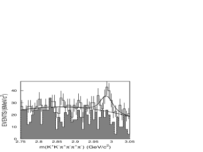
Figure 1: The distribution of $m_{K^{+}K^{-}\pi^{+}\pi^{-}\pi^{+}\pi^{-}}$ for selected events. The histogram with error bars is from data, the shaded part is the background estimated from $J/\psi\to anything$ Monte Carlo simulation, and the curve represents the fitting results described in the text.

After the above selection, the $K^{+}K^{-}\pi^{+}\pi^{-}\pi^{+}\pi^{-}$ invariant mass, $m_{K^{+}K^{-}\pi^{+}\pi^{-}\pi^{+}\pi^{-}}$, distribution is shown in Fig. 1. A peak at the $\eta_{c}$ mass is observed. The shaded histogram is the background estimated from 58 million $J/\psi\rightarrow anything$ Monte-Carlo events generated with the Lund-charm generator [10]; no prominent signal in the $\eta_{c}$ mass region is seen. Also, 100,000 events for the two possible background channels $J/\psi\rightarrow K^{+}K^{-}2(\pi^{+}\pi^{-})$ and $J/\psi\rightarrow\gamma 3(\pi^{+}\pi^{-})$ are simulated. After final selection, no events remain in the $\eta_{c}$ mass region. A Breit-Wigner folded with a Gaussian to take into account the mass resolution of 12.3 MeV/c² at the $\eta_{c}$ and a polynomial background are used in the fit. The fit gives $100\pm 26$ $\eta_{c}$ events with a statistical significance of 4.0 $\sigma$, where the mass and width of $\eta_{c}$ are fixed to the PDG values [11].

Using this sample, we search for the decay mode $\eta_{c}\rightarrow K^{*0}\overline{K}^{*0}\pi^{+}\pi^{-}$. To select $K^{*0}\overline{K}^{*0}\pi^{+}\pi^{-}$ events, we require that the invariant masses of $K^{+}\pi^{-}$ and $K^{-}\pi^{+}$ must statisfy $|m_{K\pi}-0.896|<0.05$ GeV/$c^{2}$. After the $K^{*0}$ and $\overline{K}^{*0}$ selection, the $K^{+}K^{-}2(\pi^{+}\pi^{-})$ invariant mass is shown in Fig. 2. A small peak at the $\eta_{c}$ mass is observed. The background events corresponding to the shaded histogram in Fig. 2 are estimated from $K^{*0}$ and $\overline{K}^{*0}$ sidebands (0.1 GeV/c² $<|m_{K^{+}\pi^{-}}-0.896|<0.15$ GeV/${}^{/}c^{2}$ and 0.1 GeV/c² $<|m_{K^{-}\pi^{+}}-0.896|<0.15$ GeV/${}^{/}c^{2}$), and there is no evident $\eta_{c}$ signal. $45\pm 15$ events are obtained by fitting the mass spectrum with a Breit-Wigner folded with a Gaussian to account for the $\eta_{c}$ mass resolution plus a second polynomial background. The corresponding mass and width of the $\eta_{c}$ are fixed to PDG values [11]. Since the significance of the peak is only 3$\sigma$, we also give the upper limit for $\eta_{c}\rightarrow K^{*0}\overline{K}^{*0}\pi^{+}\pi^{-}$. With the Bayes method, the fit of this distribution yields 65 events at the 90% confidence level.

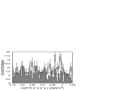
Figure 2: The distribution of $m_{K^{+}K^{-}\pi^{+}\pi^{-}\pi^{+}\pi^{-}}$ for $\eta_{c}\rightarrow K^{*0}\overline{K}^{*0}\pi^{+}\pi^{-}$ candidate events. The histogram with error bars is for data, the shaded part is the background estimated from $K^{*0}$($\overline{K}^{*0}$) sidebands, and the curve is the fitting results described in the text.

The $J/\psi\rightarrow\gamma K^{+}K^{-}\pi^{+}\pi^{-}\pi^{+}\pi^{-}$ sample can also be used to search for $\eta_{c}\rightarrow\phi\pi^{+}\pi^{-}\pi^{+}\pi^{-}$. For selecting a $\phi$ signal, the $K^{+}K^{-}$ mass, $m_{K^{+}K^{-}}$, is required to be in the region $|m_{K^{+}K^{-}}-1.02|<0.015$ GeV/c². After this selection, no clear $\eta_{c}$ signal is found in the distribution of $m_{K^{+}K^{-}\pi^{+}\pi^{-}\pi^{+}\pi^{-}}$, as shown in Fig. 3. Using Bayes method, a fit to $\eta_{c}\rightarrow K^{+}K^{-}\pi^{+}\pi^{-}\pi^{+}\pi^{-}$ with a Breit-Wigner folded with a Gaussian and a polynomial background gives 13.5 $\eta_{c}$ events at the 90% confidence level.

From Monte-carlo simulation, in which the angle ($\theta$) between the direction of the $e^{+}$ and $\eta_{c}$ in the laboratory frame is generated according to a $1+\cos^{2}\theta$ distribution and uniform phase-space is used for $\eta_{c}$ decaying into $K^{+}K^{-}2(\pi^{+}\pi^{-})$ and $\phi 2(\pi^{+}\pi^{-})$, the detection efficiencies of $J/\psi\rightarrow\gamma\eta_{c}(\eta_{c}\rightarrow K^{+}K^{-}\pi^{+}\pi^{-}\pi^{+}\pi^{-})$, $J/\psi\rightarrow\gamma\eta_{c}(\eta_{c}\rightarrow K^{*0}\overline{K}^{*0}\pi^{+}\pi^{-})$, and $J/\psi\rightarrow\gamma\eta_{c}(\eta_{c}\rightarrow\phi\pi^{+}\pi^{-}\pi^{+}\pi^{-})$ are determined as $(1.43\pm 0.04)\%$, $(1.36\pm 0.04)\%$, and $(1.01\pm 0.02)\%$, respectively. Therefore, the branching fractions obtained are

$B(J/\psi\rightarrow\gamma\eta_{c})\cdot B(\eta_{c}\rightarrow K^{+}K^{-}\pi^{+}\pi^{-}\pi^{+}\pi^{-})=(1.21\pm 0.32)\times 10^{-4}$,

$B(J/\psi\rightarrow\gamma\eta_{c})\cdot B(\eta_{c}\rightarrow K^{*0}\overline{K}^{*0}\pi^{+}\pi^{-})=(1.29\pm 0.43)\times 10^{-4}$
$B(J/\psi\rightarrow\gamma\eta_{c})\cdot B(\eta_{c}\rightarrow K^{*0}\overline{K}^{*0}\pi^{+}\pi^{-})<1.86\times 10^{-4}$,

and

$B(J/\psi\rightarrow\gamma\eta_{c})\cdot B(\eta_{c}\rightarrow\phi\pi^{+}\pi^{-}\pi^{+}\pi^{-})<4.72\times 10^{-5}$.

Figure 3: The distribution of $m_{K^{+}K^{-}\pi^{+}\pi^{-}\pi^{+}\pi^{-}}$ for $\eta_{c}\rightarrow\phi\pi^{+}\pi^{-}\pi^{+}\pi^{-}$ candidate events.

3 Analysis of $J/\psi\rightarrow\gamma\eta_{c}$,$\eta_{c}\rightarrow\pi^{+}\pi^{-}\pi^{+}\pi^{-}\pi^{+}\pi^{-}$

These events are observed in the topology $J/\psi\to\gamma\pi^{+}\pi^{-}\pi^{+}\pi^{-}\pi^{+}\pi^{-}$. Events with six good charged tracks and at least one isolated photon are selected. No particle identification is required. To suppress background, a 4C kinematic fit is performed under the hypothesis $\gamma\pi^{+}\pi^{-}\pi^{+}\pi^{-}\pi^{+}\pi^{-}$, and the $\chi^{2}$ is required to be less than 10. To reject background from $J/\psi\rightarrow{3(\pi^{+}\pi^{-})}$ and $J/\psi\rightarrow{3(\pi^{+}\pi^{-})}\pi^{0}$, we require $\chi^{2}_{\gamma\pi^{+}\pi^{-}\pi^{+}\pi^{-}\pi^{+}\pi^{-}}$ to be less than $\chi^{2}_{\pi^{+}\pi^{-}\pi^{+}\pi^{-}\pi^{+}\pi^{-}}$ and $\chi^{2}_{\pi^{+}\pi^{-}\pi^{+}\pi^{-}\pi^{+}\pi^{-}\pi^{0}}$.

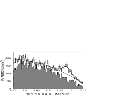
Figure 4: The distribution of $m_{\pi^{+}\pi^{-}\pi^{+}\pi^{-}\pi^{+}\pi^{-}}$ for selected events. The histogram with error bars is data, the shaded part is the background estimated from Monte Carlo simulation, and the curve is the fitting result described in the text.

Figure 4 shows the ${\pi^{+}\pi^{-}\pi^{+}\pi^{-}\pi^{+}\pi^{-}}$ invariant mass spectrum after the above selection. A clear $\eta_{c}$ peak is observed. The shaded histogram in Fig. 4 corresponds to background estimated from 58 million $J/\psi\rightarrow anything$ Monte-Carlo events generated using the Lund-Charm generator [10], where no $\eta_{c}$ signal is evident. A fit of the $m_{\pi^{+}\pi^{-}\pi^{+}\pi^{-}\pi^{+}\pi^{-}}$ distribution, which is shown as the solid curve in Fig. 4, using a Breit-Wigner convoluted with a Gaussian to represent the signal and a polynomial for the background, yields $427\pm 64$ $\eta_{c}$ events with a statistical significance of $6.9\sigma$. In the fit, the mass and width of $\eta_{c}$ are again fixed to PDG values [11].

The detection efficiency for $J/\psi\rightarrow\gamma\eta_{c},\eta_{c}\rightarrow\pi^{+}\pi^{-}\pi^{+}\pi^{-}\pi^{+}\pi^{-}$ is determined to be $(3.21\pm 0.04)\%$, by Monte-Carlo simulation with the distribution of $\theta$, the angle between the directions of $e^{+}$ and $\eta_{c}$ in the laboratory frame, being generated with a $1+\cos^{2}\theta$ and with $\eta_{c}$ decaying into $3(\pi^{+}\pi^{-})$ being generated with a uniform phase-space distribution. The branching ratio is then found to be

$B(J/\psi\rightarrow\gamma\eta_{c})\cdot B(\eta_{c}\rightarrow\pi^{+}\pi^{-}\pi^{+}\pi^{-}\pi^{+}\pi^{-})=(2.59\pm 0.32)\times 10^{-4}$.

4 Systematic errors

The systematic errors mainly come from the following sources:

(1) MDC tracking efficiency
This has been measured with clean channels like $J/\psi\rightarrow\Lambda\bar{\Lambda}$ and $\psi(2S)\rightarrow\pi^{+}\pi^{-}J/\psi,J/\psi\rightarrow\mu^{+}\mu^{-}$. It is found that the Monte Carlo simulation agrees with data within 1-2% for each charged track. Therefore, 12% is conservatively taken as the systematic error in the tracking efficiencies for the 6-prong final states analyzed here.

(2) Photon detection efficiency
This has been studied using different methods with $J/\psi\rightarrow\rho^{0}\pi^{0}$ events [12]. The difference between data and Monte Carlo simulation is less than 2% for each photon, and 2% is taken as the systematic error for the photon efficiency in this analysis.

(3) Particle identification (PID)
This has been studied with $J/\psi\rightarrow K^{+}K^{-}\pi^{0}$. The efficiency of the PID from data is consistent with that from Monte Carlo simulation. The average difference is less than 2%. For $J/\psi\rightarrow\gamma K^{+}K^{-}\pi^{+}\pi^{-}\pi^{+}\pi^{-}$ decay, 4% is taken as the systematic error from PID.

(4) Kinematic Fit
The kinematic fit is useful to reduce background. Using the same method for estimating the systematic error as in Ref. [9], the decay mode $J/\psi\rightarrow 3(\pi^{+}\pi^{-})\pi^{0}$ is also analyzed. The efficiency difference of the kinematic fit for data and Monte Carlo is 7.7%. Since the decay of $J/\psi\rightarrow 3(\pi^{+}\pi^{-})\pi^{0}$ is similar to the two channels analyzed in this paper, 7.7% is also taken here as the systematic error of the kinematic fit.

(5) $\eta_{c}$ parameters
Although the $\eta_{c}$ signal is clear, the number of events is not large enough to determine the Breit-Wigner parameters and the background shape well. The variation of the fit solution due to changes of the $\eta_{c}$ mass and width corresponding to the uncertainties in the PDG, as well as changes in the fitting mass region used, is taken as a systematic error and listed in Table 1.

(6) Background
For $\eta_{c}\rightarrow K^{+}K^{-}\pi^{+}\pi^{-}\pi^{+}\pi^{-}$, the biggest background comes from $\eta_{c}\rightarrow K^{0}_{S}K^{0}_{S}K^{+}K^{-}$. When the invariant mass of $\pi^{+}\pi^{-}$ is required to be within the $K^{0}_{S}$ mass region ($|m_{\pi^{+}\pi^{-}}-0.497|<0.02$ GeV/c²), five events remain in the $\eta_{c}$ mass region. If all of them are regarded as signal from $\eta_{c}\rightarrow K^{0}_{S}K^{0}_{S}K^{+}K^{-}$, the background from this decay mode is about 5.1%, and this is taken as the systematic error associated with background for this channel. No events remain for $\eta_{c}\rightarrow K^{*0}\overline{K}^{*0}\pi^{+}\pi^{-}$ and the upper limit is 2.3 events at 90% confidence level. Then the uncertainty caused by $\eta_{c}\rightarrow K^{0}_{S}K^{0}_{S}\pi^{+}\pi^{-}$ is 5.1%.

For the $\eta_{c}\rightarrow 3(\pi^{+}\pi^{-})$, Monte Carlo simulation is used to estimate the background from $\eta_{c}\rightarrow K^{0}_{S}K^{0}_{S}\pi^{+}\pi^{-}$. Using the branching fraction for $\eta_{c}\rightarrow K^{0}\overline{K}^{0}\pi^{+}\pi^{-}$, obtained from $B(\eta_{c}\rightarrow K^{+}K^{-}\pi^{+}\pi^{-})$ [11], Monte Carlo simulation indicates that 33 background events contribute to the $\eta_{c}$ signal. Compared to the 416 signal events from fitting the mass spectrum, the background fraction is 7.9% which is taken as the background systematic error for this channel.

(7) Number of $J/\psi$ events
The number of $J/\psi$ events is $(57.70\pm 2.72)\times 10^{6}$, determined from $J/\psi$ inclusive four-prong events. The uncertainty is taken as a systematic error in the branching ratio measurement. Table 1 lists the systematic errors from all sources, and the total systematic error is the sum of them added in quadrature.

Table 1: Systematic error sources and contributions (%)

Sources	$K^{+}K^{-}2(\pi^{+}\pi^{-})$	$K^{*0}\overline{K}^{*0}\pi^{+}\pi^{-}$	$\phi 2(\pi^{+}\pi^{-})$	$3(\pi^{+}\pi^{-})$
MDC tracking	12	12	12	12
Paticle ID	4	4	4	negligible
Photon efficiency	2	2	2	2
Kinematic fit	7.7	7.7	7.7	7.7
$\eta_{c}$ parameters	9.9	18.6	14.7	7.4
MC statistics	2.6	2.9	2.9	1.1
Background uncertainty	5.1	5.1		7.9
$B(\phi\rightarrow K^{+}K^{-})$			1.4
Number of $J/\psi$ events	4.7	4.7	4.7	4.7
Total	19.4	25.0	21.7	18.6

5 Results

The decays of $\eta_{c}\rightarrow K^{+}K^{-}\pi^{+}\pi^{-}\pi^{+}\pi^{-}$ and $\eta_{c}\rightarrow\pi^{+}\pi^{-}\pi^{+}\pi^{-}\pi^{+}\pi^{-}$ are observed for the first time, and their decay branching ratios are measured. The upper limits of $\eta_{c}\rightarrow\phi\pi^{+}\pi^{-}\pi^{+}\pi^{-}$ and $\eta_{c}\rightarrow K^{*0}\overline{K}^{*0}\pi^{+}\pi^{-}$ are also set at the 90% confidence level. To conservatively estimate the upper limit, the systematic error is included by lowering the efficiency by one standard deviation. Table 2 shows the branching ratio results including systematic errors.

Table 2: Numbers used in the calculations of branching fractions and upper limits.

Decay Modes	$N_{obs}$	$\varepsilon$ (%)	Branching Fraction
$J/\psi\rightarrow\gamma\eta_{c},\eta_{c}\rightarrow K^{+}K^{-}2(\pi^{+}\pi^{-})$	100$\pm$26	1.43$\pm$0.04	$(1.21\pm 0.32\pm 0.23)\times 10^{-4}$
$J/\psi\rightarrow\gamma\eta_{c},\eta_{c}\rightarrow K^{*0}\overline{K}^{*0}\pi^{+}\pi^{-}$	$45\pm 15$	$1.36\pm 0.04$	$(1.29\pm 0.43\pm 0.32)\times 10^{-4}$
$J/\psi\rightarrow\gamma\eta_{c},\eta_{c}\rightarrow K^{*0}\overline{K}^{*0}\pi^{+}\pi^{-}$	$<65$	$1.36\pm 0.04$	$<2.46\times 10^{-4}$ (90% C.L.)
$J/\psi\rightarrow\gamma\eta_{c},\eta_{c}\rightarrow\phi 2(\pi^{+}\pi^{-})$	$<13.5$	$1.01\pm 0.02$	$<6.03\times 10^{-5}$ (90% C.L.)
$J/\psi\rightarrow\gamma\eta_{c},\eta_{c}\rightarrow 3(\pi^{+}\pi^{-})$	427$\pm$64	3.21$\pm$0.04	$(2.59\pm 0.32\pm 0.48)\times 10^{-4}$

Using the branching fraction of $J/\psi\rightarrow\gamma\eta_{c}$ as $B(J/\psi\rightarrow\gamma\eta_{c})=(1.3\pm 0.4)\%$ from the PDG [11], we obtain:

$B(\eta_{c}\rightarrow K^{+}K^{-}\pi^{+}\pi^{-}\pi^{+}\pi^{-})=(0.93\pm 0.25\pm 0.34)\times 10^{-2}$

$B({\eta_{c}}\rightarrow K^{*0}\overline{K}^{*0}\pi^{+}\pi^{-})=(0.99\pm 0.33\pm 0.39)\times 10^{-2}$

$B({\eta_{c}}\rightarrow K^{*0}\overline{K}^{*0}\pi^{+}\pi^{-})<2.36\times 10^{-2}$

$B(\eta_{c}\rightarrow\phi\pi^{+}\pi^{-}\pi^{+}\pi^{-})<5.81\times 10^{-3}$ (90% C.L.)

$B({\eta_{c}}\rightarrow{\pi^{+}\pi^{-}\pi^{+}\pi^{-}\pi^{+}\pi^{-}})=(1.99\pm 0.25\pm 0.72)\times 10^{-2}$

The BES collaboration thanks the staff of BEPC and the computing center for their hard efforts. This work is supported in part by the National Natural Science Foundation of China under contracts Nos. 19991480, 10225524, 10225525, the Chinese Academy of Sciences under contract No. KJ 95T-03, the 100 Talents Program of CAS under Contract Nos. U-11, U-24, U-25, and the Knowledge Innovation Project of CAS under Contract Nos. U-602, U-34 (IHEP); and by the National Natural Science Foundation of China under Contract No.10175060 (USTC), and No. 10225522 (Tsinghua University); and by the U. S. Department of Energy under Contract N0. DE-FG02-04ER41291.

References

- [1] P. Partridge et al., Phys. Rev. Lett. 45 (1980) 1150.
- [2] T. Himel et al.m, Phys. Rev. Lett. 45 (1980) 1146.
- [3] R. M. Baltrusaitis et al., Phys. Rev.D33 (1986) 629; D. Bisello et al.,Phys. Lett. 179B (1986) 294; D. Bisello et al., Phys. Lett. 192B (1987) 294; J. Z. Bai et al., Phys. Rev. D62 (2000) 072001.
- [4] J.Z. Bai et al., Phys. Lett. B555 (2003) 174; J.Z. Bai et al., Phys. Lett. B578 (2004)16; H.-C Huang et al., hep-ex/0305068; F. Fang et al., Phys. Rev. Lett. 90 (2003) 071801; B. Aubert et al., Phys. Rev. D70 (2004) 011101.
- [5] C. Quigg and J. L. Rosner, Phys. Rev. D16 (1977) 1497.
- [6] S. S. Fang et al., High Energy Phys. Nucl. Phys. 27 (2003) 277(in Chinese).
- [7] J. Z. Bai et al., Nucl. Instrum. Methods A 458 (2001) 627.
- [8] BES Collaboration, physics/0503001. Accepted by Nucl. Instrum. Methods A.
- [9] J. Z. Bai et al., Phys. Rev. D70 (2004) 012005.
- [10] J. C. Chen et al., Phys. Rev. D62 (2000) 034003.
- [11] S. Eidelman et al., Phys. Lett. B592 (2004) 1.
- [12] S. M. Li et al., High Energy Phys. Nucl. Phys. 28 (2004) 859(in Chinese).