Study of $\Lambda^{+}_{c}$ Cabibbo Favored Decays Containing a $\Lambda$ Baryon in the Final State

Abstract

Using data from the FOCUS experiment (FNAL-E831), we study the decay of $\Lambda^{+}_{c}$ baryons into final states containing a $\Lambda$ hyperon. The branching fractions of $\Lambda^{+}_{c}$ into $\Lambda\pi^{+}$, $\Lambda\pi^{+}\pi^{+}\pi^{-}$ and $\Lambda\overline{K}\,\!^{0}K^{+}$ relative to that into $pK^{-}\pi^{+}$ are measured to be $0.217\pm 0.013\pm 0.020$, $0.508\pm 0.024\pm 0.024$ and $0.142\pm 0.018\pm 0.022$, respectively. We also report new measurements of $\frac{\Gamma(\Lambda^{+}_{c}\rightarrow\Sigma^{0}\pi^{+})}{\Gamma(\Lambda^{+}_{c}\rightarrow\Lambda\pi^{+})}=1.09\pm 0.11\pm 0.19$, $\frac{\Gamma(\Lambda^{+}_{c}\rightarrow\Sigma^{0}\pi^{+}\pi^{+}\pi^{-})}{\Gamma(\Lambda^{+}_{c}\rightarrow\Lambda\pi^{+}\pi^{+}\pi^{-})}=0.26\pm 0.06\pm 0.09$ and $\frac{\Gamma(\Lambda^{+}_{c}\rightarrow\Xi(1690)^{0}(\Lambda\overline{K}\,\!^{0})K^{+})}{\Gamma(\Lambda^{+}_{c}\rightarrow\Lambda\overline{K}\,\!^{0}K^{+})}=0.33\pm 0.10\pm 0.04$. Further, an analysis of the subresonant structure for the $\Lambda^{+}_{c}\rightarrow\Lambda\pi^{+}\pi^{+}\pi^{-}$ decay mode is presented.

The FOCUS Collaboration

1 Introduction

During the past several years there has been significant progress in the experimental study of hadronic decays of charmed baryons. However the precision on branching fraction measurements is only about 40% for many Cabibbo-favored modes and even worse for Cabibbo-suppressed decays [1]. As a result, we are not yet able to distinguish between the decay rate predictions made by different theoretical models, e.g., the quark model approach to non-leptonic charm decays and the Heavy Quark Effective Theory (HQET) [2, 3, 4]. In this paper we present a study of $\Lambda^{+}_{c}$ baryons produced by the FOCUS experiment. We present improved measurements of the branching fractions of the Cabibbo-favored decays $\Lambda^{+}_{c}\rightarrow\Lambda\pi^{+},\Lambda^{+}_{c}\rightarrow\Lambda\pi^{+}\pi^{+}\pi^{-}$ and $\Lambda^{+}_{c}\rightarrow\Lambda\overline{K}\,\!^{0}K^{+}$. From the measurement of the first two modes, we are also able to extract the relative branching ratios of the two decays $\Lambda^{+}_{c}\rightarrow\Sigma^{0}\pi^{+}$ and $\Lambda^{+}_{c}\rightarrow\Sigma^{0}\pi^{+}\pi^{+}\pi^{-}$. We report a new measurement of the subresonant mode $\Lambda^{+}_{c}\rightarrow\Xi(1690)^{0}K^{+}$. Finally we present the first study of the subresonant structure of the $\Lambda^{+}_{c}\rightarrow\Lambda\pi^{+}\pi^{+}\pi^{-}$ decay mode.

2 Event Reconstruction

This analysis uses data collected by the FOCUS experiment during the 1996–1997 fixed-target run at Fermilab.

FOCUS is a photo-production experiment equipped with very precise vertexing and particle identification detectors. The vertexing system is composed of a silicon microstrip detector (TS) embedded in the BeO target segments [5], and a second system of twelve microstrip planes (SSD) downstream of the target. Downstream of the SSD, five stations of multiwire proportional chambers and two large aperture dipole magnets complete the charged particle tracking and momentum measurement system. Three multicell threshold Čerenkov detectors are used to identify electrons, pions, kaons, and protons. The FOCUS apparatus also contains one hadronic and two electromagnetic calorimeters as well as two muon detectors.

All decay modes reported have a $\Lambda$ hyperon in the final state. A detailed description of $\Lambda$ and $K^{0}_{S}$ reconstruction techniques in FOCUS is reported in Reference [6].

Candidates are reconstructed by first forming a vertex with tracks consistent with a specific $\Lambda^{+}_{c}$ decay hypothesis. A cut on the confidence level that these tracks form a good vertex is applied. Production vertex candidates are found using a candidate driven vertexing algorithm which uses the $\Lambda^{+}_{c}$ candidate momentum to define the line of the flight of the charm particle [7]. This seed track is intersected with other tracks in the event to form a production vertex. The confidence level for the production vertex must be greater than 1%. Most of the background is rejected by applying a separation cut between the production and decay vertices: we require the significance of separation between the two vertices, $L/\sigma_{L}$, to be greater than some number, depending on the decay mode.

All charged microstrip track segments from the charm decay must be linked to a single multi-wire proportional chamber track segment, be of good quality, and be inconsistent with zero degree tracks from photon conversion. The likelihood for each charged particle to be proton, kaon, pion or electron based on Čerenkov particle identification is used to make additional requirements [8]. For pion candidates, we require a loose cut that no alternative hypothesis is favored over the pion hypothesis by more than 6 units of log-likelihood. In addition, for each kaon candidate we require the negative log-likelihood kaon hypothesis, $W_{K}=-2\ln$ (kaon likelihood), to be favored over the corresponding pion hypothesis $W_{\pi}$ by $W_{\pi}-W_{K}>3$.

The reconstructed mass of the $\Lambda$ candidates must be between 1.1 and 1.125 GeV/$c^{2}$; no cut is applied on the normalized mass $[M(\Lambda)-M(\Lambda)_{PDG}]/\sigma_{M(\Lambda)}$, because it is not centered around zero, probably due to the higher background under the signal region. We moreover require the higher momentum track used to reconstruct the $\Lambda$ candidates to be compatible with the proton hypothesis, applying the cut $W_{\pi}-W_{p}>4$. The reconstructed mass of the $K^{0}_{S}$ must be within three standard deviations of the nominal $K^{0}_{S}$ mass.

We require $\Lambda^{+}_{c}$ candidates to have a minimum momentum of 45 GeV/$c$ and to have a lifetime less than five times the nominal value [1]. Finally, in order to reduce backgrounds, we require the production vertex to be located inside the target material.

3 The normalization mode

The $\Lambda^{+}_{c}\rightarrow pK^{-}\pi^{+}$ channel is our highest statistics $\Lambda^{+}_{c}$ decay mode and it is used as the normalization mode for branching ratio measurements to minimize the overall statistical uncertainty. Moreover, all previous measurements in the literature [1] use this decay as a normalization mode, thus making any comparison straightforward.

In order to minimize systematic biases, the normalization mode is selected using the same cuts and the same fitting technique as the specific decay whenever possible. In addition, for each proton candidate we apply the cuts $W_{\pi}-W_{p}>4$ and $W_{K}-W_{p}>1$. The $pK^{-}\pi^{+}$ invariant mass distribution for an $L/\sigma_{L}>4$ cut is shown in Fig. 1 (b). The resultant yield is $16447\pm 193$ events.

4 The $\Lambda^{+}_{c}\rightarrow\Lambda\pi^{+}$ decay mode

We measure the branching ratio of $\Lambda^{+}_{c}\rightarrow\Lambda\pi^{+}$ relative to $\Lambda^{+}_{c}\rightarrow pK^{-}\pi^{+}$. In Fig. 1 (a) the $\Lambda\pi^{+}$ invariant mass distribution for an $L/\sigma_{L}>4$ cut is presented. The confidence level for the decay vertex must be greater than 1%. We also apply a $|\cos\theta|<$ 0.6 cut, where $\theta$ is the angle between the $\Lambda$ momentum in the $\Lambda^{+}_{c}$ rest frame and the $\Lambda^{+}_{c}$ laboratory momentum.

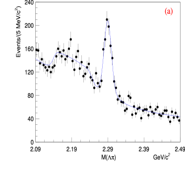
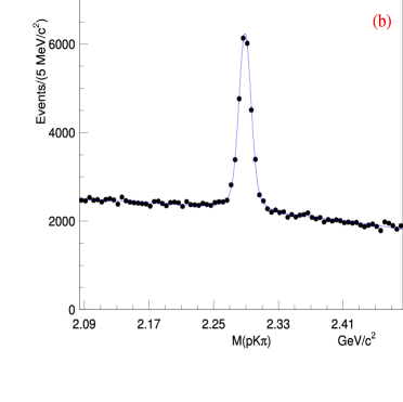
Figure 1: Invariant mass distributions for (a) $\Lambda^{+}_{c}\rightarrow\Lambda\pi^{+}$ and (b) $\Lambda^{+}_{c}\rightarrow pK^{-}\pi^{+}$. The fits are described in the text.

We note a broad structure around 2.2 GeV/$c^{2}$ coming from the decay mode $\Lambda^{+}_{c}\rightarrow\Sigma^{0}(\Lambda\gamma)\pi^{+}$ where the photon from the $\Sigma^{0}$ decay is not reconstructed. The shape for this reflection has been obtained from a Monte Carlo simulation of this decay mode. The fit is performed using two Gaussians with the same mean for the signal, the reflection from the $\Sigma^{0}\pi^{+}$ mode, and a second order Chebychev polynomial for the background. The ratio of yields and the resolutions of the two Gaussians are fixed to the Monte Carlo values. The resultant yield is $750\pm 44$ events. Correcting for the relative efficiencies estimated by our Monte Carlo simulation, we determine the branching ratio to be

$$\frac{\Gamma(\Lambda^{+}_{c}\rightarrow\Lambda\pi^{+})}{\Gamma(\Lambda^{+}_{c}\rightarrow pK^{-}\pi^{+})}=0.217\pm 0.013~{}(\mbox{stat.}).$$ (1)

The number of fitted $\Lambda^{+}_{c}\rightarrow\Sigma^{0}\pi^{+}$ reflection events is 919 $\pm$ 92. Correcting for the relative efficiencies, we extract the relative branching ratio:

$$\frac{\Gamma(\Lambda^{+}_{c}\rightarrow\Sigma^{0}\pi^{+})}{\Gamma(\Lambda^{+}_{c}\rightarrow\Lambda\pi^{+})}=1.09\pm 0.11~{}(\mbox{stat.}).$$ (2)

5 The $\Lambda^{+}_{c}\rightarrow\Lambda\pi^{+}\pi^{+}\pi^{-}$ decay mode

We measure the branching ratio of $\Lambda^{+}_{c}\rightarrow\Lambda\pi^{+}\pi^{+}\pi^{-}$ relative to $\Lambda^{+}_{c}\rightarrow pK^{-}\pi^{+}$. In Fig. 2 (a) the $\Lambda\pi^{+}\pi^{+}\pi^{-}$ invariant mass distribution for an $L/\sigma_{L}>5$ cut is presented. The confidence level for the decay vertex must be greater than 5%. We also apply a $\cos\theta>-0.9$ cut, where $\theta$ is the angle between the $\Lambda$ momentum in the $\Lambda^{+}_{c}$ rest frame and the $\Lambda^{+}_{c}$ laboratory momentum.

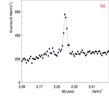
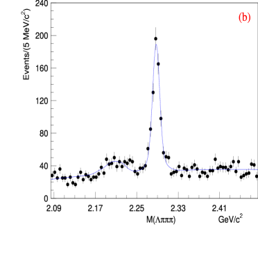
Figure 2: Invariant mass distributions for (a) $\Lambda^{+}_{c}\rightarrow\Lambda\pi^{+}\pi^{+}\pi^{-}$ and (b) $\Lambda^{+}_{c}\rightarrow\Lambda\pi^{+}\pi^{+}\pi^{-}$ for the subresonant analysis. The fits are described in the text.

We also note in this decay mode a broad structure around 2.2 GeV/$c^{2}$ coming from the decay mode $\Lambda^{+}_{c}\rightarrow\Sigma^{0}(\Lambda\gamma)\pi^{+}\pi^{+}\pi^{-}$ where the photon from the $\Sigma^{0}$ decay has not been reconstructed. This has been accounted for as in the $\Lambda^{+}_{c}\rightarrow\Lambda\pi^{+}$ decay. The components of the fitting function are the same as in the $\Lambda^{+}_{c}\rightarrow\Lambda\pi^{+}$ case. The resultant $\Lambda^{+}_{c}\rightarrow\Lambda\pi^{+}\pi^{+}\pi^{-}$ yield is $1356\pm 60$ events. Correcting for the relative efficiencies estimated by our Monte Carlo simulation, we determine the branching ratio to be

$$\frac{\Gamma(\Lambda^{+}_{c}\rightarrow\Lambda\pi^{+}\pi^{+}\pi^{-})}{\Gamma(\Lambda^{+}_{c}\rightarrow pK^{-}\pi^{+})}=0.508\pm 0.024~{}(\mbox{stat.}).$$ (3)

The number of fitted $\Lambda^{+}_{c}\rightarrow\Sigma^{0}\pi^{+}\pi^{+}\pi^{-}$ reflection events is 480 $\pm$ 110. Correcting for the relative efficiencies, we extract the relative branching ratio:

$$\frac{\Gamma(\Lambda^{+}_{c}\rightarrow\Sigma^{0}\pi^{+}\pi^{+}\pi^{-})}{\Gamma(\Lambda^{+}_{c}\rightarrow\Lambda\pi^{+}\pi^{+}\pi^{-})}=0.26\pm 0.06~{}(\mbox{stat.}).$$ (4)

We have studied the subresonant structure in the decay mode $\Lambda^{+}_{c}\rightarrow\Lambda\pi^{+}\pi^{+}\pi^{-}$. Considering our limited statistics, which would make a coherent analysis difficult, we use an incoherent binned fit method [9] developed by the E687 Collaboration, which assumes the final state is an incoherent superposition of subresonant decay modes.

For the resonant substructure analysis of $\Lambda^{+}_{c}\rightarrow\Lambda\pi^{+}\pi^{+}\pi^{-}$ we enhance the signal to noise ratio applying an $L/\sigma_{L}>8$ cut and requiring $1.11<M(\Lambda)<1.119$ GeV/$c^{2}$. In Fig. 2 (b) the $\Lambda\pi^{+}\pi^{+}\pi^{-}$ invariant mass distribution for events which satisfy these cuts is presented. The resultant yield is $594\pm 31$ events.

A study of the two-body invariant mass distributions was done to better identify which resonances may contribute to the $\Lambda\pi^{+}\pi^{+}\pi^{-}$ decay channel. In Fig. 3 the two body $\Lambda\pi^{-}$, $\Lambda\pi^{+}$ and $\pi^{+}\pi^{-}$ invariant mass distributions provide evidence for the $\Sigma(1385)^{\pm}$ and $\rho(770)^{0}$ resonances. For this study we require the $\Lambda\pi^{+}\pi^{+}\pi^{-}$ invariant mass to be within 2$\sigma$ (18 MeV/$c^{2}$) of the $\Lambda^{+}_{c}$ nominal mass and we perform a sideband subtraction to reduce the background. The fits are performed using Breit-Wigners for the signal shape, with the mean and width fixed to the Monte Carlo values, and Chebychev polynomials for the backgrounds.

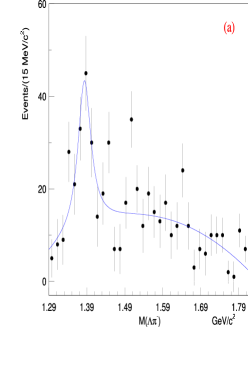
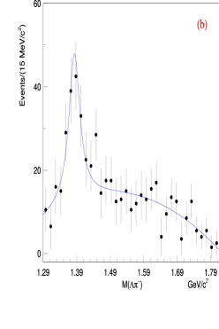
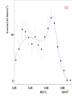
Figure 3: (a) $\Lambda\pi^{-}$, (b) $\Lambda\pi^{+}$ and (c) $\pi^{+}\pi^{-}$ invariant mass distributions in the decay mode $\Lambda^{+}_{c}\rightarrow\Lambda\pi^{+}\pi^{+}\pi^{-}$. The yields are, respectively, 143 $\pm$ 27, 149 $\pm$ 28 and 317 $\pm$ 68.

For subresonant modes in the resonant analysis we therefore consider the channels $\Sigma(1385)^{-}\pi^{+}\pi^{+}$, $\Sigma(1385)^{+}\pi^{+}\pi^{-}$, $\Lambda\rho(770)^{0}\pi^{+}$ and $\Sigma(1385)^{+}\rho(770)^{0}$, plus a nonresonant channel $(\Lambda\pi^{+}\pi^{+}\pi^{-})_{NR}$. All states not explicitly considered are assumed to be included in the nonresonant channel.

We determine the acceptance corrected yield into each subresonant mode using a weighting technique whereby each event is weighted by its kinematic values in the three submasses ($\Lambda\pi^{-}$), ($\Lambda\pi^{+}$) and ($\pi^{+}\pi^{-}$). We construct eight population bins depending on whether each of the three submasses falls into the expected resonance peak (within the nominal width). From a Monte Carlo simulation of each subresonant mode $\alpha$, we compute the bin population $n_{i}$ in the eight bins and we calculate a transport matrix $T_{i\alpha}$ between the number of generated Monte Carlo events $Y_{\alpha}$ and the bin populations:

$$n_{i}=\sum_{\alpha}T_{i\alpha}Y_{\alpha}.$$ (5)

The elements of the $T$ matrix can be summed to give the efficiency $\epsilon_{\alpha}$ for each mode:

$$\centering\epsilon_{\alpha}=\sum_{i}T_{i\alpha}.\@add@centering$$ (6)

This Monte Carlo determined matrix is inverted to create a new weighting matrix which multiplies the bin populations to produce efficiency corrected yields. Each data event can then be weighted according to its values in the submass bins. Once the weighted distributions for each of the five modes have been generated, we determine the acceptance corrected yields by fitting the distributions with two Gaussians with the same mean and a second order Chebychev polynomial for the background. Using incoherent Monte Carlo mixtures of the five subresonant modes we verify that the method is able to correctly reproduce the generated mixtures of the different modes.

The results for the $\Lambda\pi^{+}\pi^{+}\pi^{-}$ decay are summarized in Table 1. The five weighted histograms are shown in Fig. 4, where Fig. 4 (f) is the weighted distribution for the sum of all subresonant modes. The systematic uncertainty for the subresonant fractions is estimated varying the width of the resonance peaks in the construction of the kinematic bins. The goodness of fit is evaluated by calculating a $\chi^{2}$ for the hypothesis of consistency between the model predictions and the observed data yields in each of the 8 submass bins. We obtain a $\chi^{2}$ of 7.86 (for 3 degrees of freedom) and a confidence level of about 5%.

Table 1: Fractions relative to the inclusive mode for the subresonant structure of the $\Lambda^{+}_{c}\rightarrow\Lambda\pi^{+}\pi^{+}\pi^{-}$ decay mode.

Subresonant Mode	Fraction of $\Lambda^{+}_{c}\rightarrow\Lambda\pi^{+}\pi^{+}\pi^{-}$
$(\Lambda\pi^{+}\pi^{+}\pi^{-})_{NR}$	$<$ 0.30 @90% CL
$\Sigma^{*-}\pi^{+}\pi^{+}$	0.21 $\pm$ 0.03 $\pm$ 0.02
$\Sigma^{*+}\pi^{+}\pi^{-}$	0.28 $\pm$ 0.10 $\pm$ 0.08
$\Lambda\pi^{+}\rho$	0.40 $\pm$ 0.12 $\pm$ 0.12
$\Sigma^{*+}\rho$	0.14 $\pm$ 0.09 $\pm$ 0.07

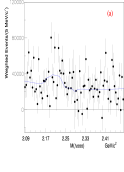
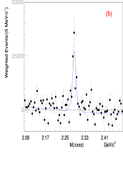
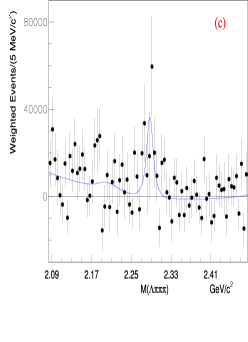
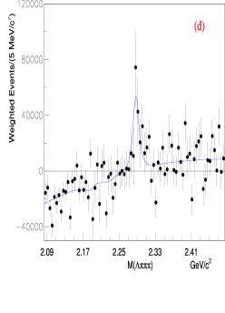
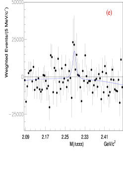
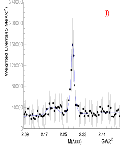
Figure 4: $\Lambda^{+}_{c}\rightarrow\Lambda\pi^{+}\pi^{+}\pi^{-}$ weighted invariant mass distributions for (a) $(\Lambda\pi^{+}\pi^{+}\pi^{-})_{NR}$, (b) $\Sigma(1385)^{-}\pi^{+}\pi^{+}$, (c) $\Sigma(1385)^{+}\pi^{+}\pi^{-}$, (d) $\Lambda\rho(770)^{0}\pi^{+}$, (e) $\Sigma(1385)^{+}\rho(770)^{0}$, (f) inclusive sum of all five modes.

6 The $\Lambda^{+}_{c}\rightarrow\Lambda\overline{K}\,\!^{0}K^{+}$ decay mode

We measure the branching ratio of $\Lambda^{+}_{c}\rightarrow\Lambda\overline{K}\,\!^{0}K^{+}$ relative to $\Lambda^{+}_{c}\rightarrow pK^{-}\pi^{+}$. The $\overline{K}\,\!^{0}$ are detected through $K^{0}_{S}$’s. Due to the limited phase space, the signal can be observed without the need for a $L/\sigma_{L}$ or decay vertex confidence level cut. In Fig. 5 the $\Lambda K^{0}_{S}K^{+}$ invariant mass distribution is presented.

The fit is performed using two Gaussians with the same mean for the signal and a second order Chebychev polynomial for the background. The ratio of yields and the resolutions of the two Gaussians are fixed to the Monte Carlo values. The resultant yield is $251\pm 31$ events. Correcting for the relative efficiencies estimated by our Monte Carlo simulation, we determine the branching ratio to be

$$\frac{\Gamma(\Lambda^{+}_{c}\rightarrow\Lambda\overline{K}\,\!^{0}K^{+})}{\Gamma(\Lambda^{+}_{c}\rightarrow pK^{-}\pi^{+})}=0.142\pm 0.018~{}(\mbox{stat.}).$$ (7)

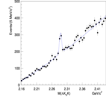
Figure 5: Invariant mass distribution for $\Lambda^{+}_{c}\rightarrow\Lambda K^{0}_{S}K^{+}$. The fit is described in the text.

The Belle collaboration [10] has recently shown evidence of the resonant contribution $\Lambda^{+}_{c}\rightarrow\Xi(1690)^{0}K^{+}$ in the decay $\Lambda^{+}_{c}\rightarrow\Lambda K^{0}_{S}K^{+}$ with the $\Xi(1690)^{0}$ reconstructed in $\Lambda K^{0}_{S}$. In our analysis, the $\Xi(1690)^{0}K^{+}$ events are selected using the same cuts used for the $\Lambda K^{0}_{S}K^{+}$ mode; the $\Lambda K^{0}_{S}K^{+}$ invariant mass is required to be within 2$\sigma$ (10 MeV/$c^{2}$) of the $\Lambda^{+}_{c}$ nominal mass. A sideband subtraction is performed to reduce the combinatoric background under the $\Lambda^{+}_{c}$ signal region.

The $\Lambda K^{0}_{S}$ invariant mass distribution is shown in Fig. 6. The fit is performed using a Breit-Wigner function for the signal and a first order Chebychev polynomial for the background. The mean and the width of the Breit-Wigner are fixed to the Monte Carlo values. The resultant yield is $84\pm 24$ events.

We measure the branching ratio relative to $\Lambda^{+}_{c}\rightarrow\Lambda\overline{K}\,\!^{0}K^{+}$ to be

$$\frac{\Gamma(\Lambda^{+}_{c}\rightarrow\Xi(1690)^{0}K^{+})}{\Gamma(\Lambda^{+}_{c}\rightarrow\Lambda\overline{K}\,\!^{0}K^{+})}\times B(\Xi(1690)^{0}\rightarrow\Lambda\overline{K}\,\!^{0})=0.33\pm 0.10~{}(\mbox{stat.}).$$ (8)

7 Systematic studies

The systematic effects are evaluated after investigation of different sources: uncertainties in the reconstruction efficiency and in the resonant substructure for multibody decays and the choice of fitting conditions.

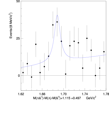
Figure 6: Invariant mass distribution for $\Lambda K^{0}_{S}$ in the decay $\Lambda^{+}_{c}\rightarrow\Lambda K^{0}_{S}K^{+}$. The fit is described in the text.

To determine the systematic error due to the reconstruction efficiency we follow a procedure based on the S-factor method used by the Particle Data Group [1]. For each mode we split the data sample into independent subsamples based on $\Lambda^{+}_{c}$ momentum, data-taking period, particle-antiparticle, significance of separation between production and decay vertices and different $\Lambda$ and $K^{0}_{S}$ categories, based on the location and geometry of the neutral particle decay. These splits provide a check on the Monte Carlo simulation of charm production, of the vertex detector and of different variables employed in the event selection. We define the split sample variance as the difference between the scaled variance and the statistical variance if the former exceeds the latter. The method is described in detail in Reference [11].

Considering the large uncertainty on the measured subresonant fractions in the multibody decays, we also vary these fractions in the Monte Carlo simulation and we use the variance in the branching ratios as a contribution to the systematic error.

We measure the systematic uncertainty due to fitting conditions using a fit variation technique, which includes variations in bin size, fitting range, background and signal shapes (different order of the Chebychev polynomial, leaving the two Gaussian parameters free in the fit or using a single Gaussian for the signal).

We also include a systematic error contribution from the absolute tracking efficiency for the different multiplicities in the final states. In Table 2 we summarize the systematic uncertainty for each mode. Several measurements for the modes reported here are present in the literature [12, 13, 14, 15, 16, 17, 18]. In Table 3 we present the FOCUS results with a comparison to the PDG values [1].

Table 2: The systematic uncertainties from the Monte Carlo simulation, the fitting condition and the the total for each mode.

Mode	Simulation	Subresonances	Tracking	Fit	Total
$\frac{\Gamma(\Lambda^{+}_{c}\rightarrow\Lambda\pi^{+})}{\Gamma(\Lambda^{+}_{c}\rightarrow pK^{-}\pi^{+})}$	0.017	—	0.005	0.008	0.020
$\frac{\Gamma(\Lambda^{+}_{c}\rightarrow\Sigma^{0}\pi^{+})}{\Gamma(\Lambda^{+}_{c}\rightarrow\Lambda\pi^{+})}$	0.19	—	—	0.04	0.19
$\frac{\Gamma(\Lambda^{+}_{c}\rightarrow\Lambda\pi^{+}\pi^{+}\pi^{-})}{\Gamma(\Lambda^{+}_{c}\rightarrow pK^{-}\pi^{+})}$	0.016	0.010	—	0.014	0.024
$\frac{\Gamma(\Lambda^{+}_{c}\rightarrow\Sigma^{0}\pi^{+}\pi^{+}\pi^{-})}{\Gamma(\Lambda^{+}_{c}\rightarrow\Lambda\pi^{+}\pi^{+}\pi^{-})}$	0.08	—	—	0.03	0.09
$\frac{\Gamma(\Lambda^{+}_{c}\rightarrow\Lambda\overline{K}\,\!^{0}K^{+})}{\Gamma(\Lambda^{+}_{c}\rightarrow pK^{-}\pi^{+})}$	0.021	0.001	0.004	0.005	0.022
$\frac{\Gamma(\Lambda^{+}_{c}\rightarrow\Xi(1690)^{0}(\Lambda\overline{K}\,\!^{0})K^{+})}{\Gamma(\Lambda^{+}_{c}\rightarrow\Lambda\overline{K}\,\!^{0}K^{+})}$	—	—	—	0.04	0.04

8 Conclusions

We have investigated and measured the branching ratios of several $\Lambda^{+}_{c}$ Cabibbo-favored decay modes containing the $\Lambda$ hyperon in the final state. These modes are $\Lambda^{+}_{c}\rightarrow\Lambda\pi^{+},\Lambda^{+}_{c}\rightarrow\Lambda\pi^{+}\pi^{+}\pi^{-}$ and $\Lambda^{+}_{c}\rightarrow\Lambda\overline{K}\,\!^{0}K^{+}$. From the fit to the first two modes, we are also able to extract the relative branching ratios of the two decays $\Lambda^{+}_{c}\rightarrow\Sigma^{0}\pi^{+}$ and $\Lambda^{+}_{c}\rightarrow\Sigma^{0}\pi^{+}\pi^{+}\pi^{-}$. These measurements are an improvement over previous results for the same decay modes. We report a new measurement of the subresonant mode $\Lambda^{+}_{c}\rightarrow\Xi(1690)^{0}K^{+}$ consistent with the recent Belle result. We have also performed an analysis of the subresonant structure of the decay $\Lambda^{+}_{c}\rightarrow\Lambda\pi^{+}\pi^{+}\pi^{-}$. We observe a small nonresonant component and the presence of vector resonances in the dominant modes, as it has been observed in most charm meson decays.

9 Acknowledgments

We wish to acknowledge the assistance of the staffs of Fermi National Accelerator Laboratory, the INFN of Italy, and the physics departments of the collaborating institutions. This research was supported in part by the U. S. National Science Foundation, the U. S. Department of Energy, the Italian Istituto Nazionale di Fisica Nucleare and Ministero dell’Istruzione, dell’Università e della Ricerca, the Brazilian Conselho Nacional de Desenvolvimento Científico e Tecnológico, CONACyT-México, and the Korea Research Foundation of the Korean Ministry of Education.

Table 3: FOCUS results compared to previous measurements. No direct measurement exists for the relative branching ratios $\Gamma(\Lambda^{+}_{c}\rightarrow\Sigma^{0}\pi^{+})/\Gamma(\Lambda^{+}_{c}\rightarrow\Lambda\pi^{+})$ and $\Gamma(\Lambda^{+}_{c}\rightarrow\Sigma^{0}\pi^{+}\pi^{+}\pi^{-})/\Gamma(\Lambda^{+}_{c}\rightarrow\Lambda\pi^{+}\pi^{+}\pi^{-})$. The relative efficiency includes the branching fractions into the observed final state particles.

$\Lambda^{+}_{c}$ Decay	Signal	$\Lambda^{+}_{c}$ Reference	Reference	Relative	FOCUS	PDG [1]
Mode	Yield	Mode	Yield	Efficiency
$\Lambda\pi^{+}$	750 $\pm$ 44	$pK^{-}\pi^{+}$	16447 $\pm$ 193	0.209 $\pm$ 0.001	0.217 $\pm$ 0.013 $\pm$ 0.020	0.180 $\pm$ 0.032
$\Sigma^{0}\pi^{+}$	919 $\pm$ 92	$\Lambda\pi^{+}$	750 $\pm$ 44	1.119 $\pm$ 0.001	1.09 $\pm$ 0.11 $\pm$ 0.19	1.11 $\pm$ 0.49
$\Lambda\pi^{+}\pi^{+}\pi^{-}$	1356 $\pm$ 60	$pK^{-}\pi^{+}$	12898 $\pm$ 147	0.207 $\pm$ 0.001	0.508 $\pm$ 0.024 $\pm$ 0.024	0.66 $\pm$ 0.11
$\Sigma^{0}\pi^{+}\pi^{+}\pi^{-}$	480 $\pm$ 110	$\Lambda\pi^{+}\pi^{+}\pi^{-}$	1356 $\pm$ 60	1.375 $\pm$ 0.001	0.26 $\pm$ 0.06 $\pm$ 0.09	0.33 $\pm$ 0.16
$\Lambda\overline{K}\,\!^{0}K^{+}$	251 $\pm$ 31	$pK^{-}\pi^{+}$	10952 $\pm$ 132	0.161 $\pm$ 0.001	0.142 $\pm$ 0.018 $\pm$ 0.022	0.12 $\pm$ 0.02 $\pm$ 0.02
$\Xi(1690)^{0}(\Lambda\overline{K}\,\!^{0})K^{+}$	84 $\pm$ 24	$\Lambda\overline{K}\,\!^{0}K^{+}$	251 $\pm$ 31	1.00	0.33 $\pm$ 0.10 $\pm$ 0.04	0.26 $\pm$ 0.08 $\pm$ 0.03

References

- [1] S. Eidelman et al., Particle Data Group, Phys. Lett. B592 (2004) 1.
- [2] T. Utpal, R. C. Verma and M. P. Khana, Phys. Rev. D49 (1994) 3417.
- [3] J. G. Körner and M. Krämer, Z. Phys. C55 (1992) 659.
- [4] J. G. Körner, M. Krämer and J. Willrodt, Z. Phys. C2 (1979) 117.
- [5] J. M. Link et al., FOCUS Collaboration, Nucl. Instrum. Meth. A516 (2004) 364.
- [6] J. M. Link et al., FOCUS Collaboration, Nucl. Instrum. Meth. A484 (2002) 174.
- [7] P. L. Frabetti et al., E687 Collaboration, Nucl. Instrum. Meth. A320 (1992) 519.
- [8] J. M. Link et al., FOCUS Collaboration, Nucl. Instrum. Meth. A484 (2002) 270.
- [9] P. L. Frabetti et al., E687 Collaboration, Phys. Lett. B354 (1995) 486.
- [10] K. Abe et al., Belle Collaboration, Phys. Lett. B524 (2002) 33.
- [11] J. M. Link et al., FOCUS Collaboration, Phys. Lett. B555 (2003) 167.
- [12] H. Albrecht et al. ARGUS Collaboration, Phys. Lett. B274 (1992) 239.
- [13] P. Avery et al. CLEO Collaboration, Phys. Rev. D43 (1991) 3599.
- [14] J. C. Anjos et al. E691 Collaboration, Phys. Rev. D41 (1990) 801.
- [15] H. Albrecht et al. ARGUS Collaboration, Phys. Lett. B207 (1988) 109.
- [16] S. Barlag et al. ACCMOR Collaboration, Z. Phys. C48 (1990) 29.
- [17] P. Avery et al. CLEO Collaboration, Phys. Lett. B325 (1994) 257.
- [18] R. Ammar et al. CLEO Collaboration, Phys. Rev. Lett. 74 (1995) 3534.