Search for new physics in B to VV decays and other hot topics from Belle

We report studies in polarization in $B$ decay into two vector mesons with data equivalent to $253{\rm fb^{-1}}$ on $\Upsilon(4S)$ resonance at KEKB. In $B^{0}\to\phi K^{*0}$, $B^{+}\to\phi K^{*+}$ and $B^{+}\to\rho^{+}K^{*0}$ decays, we determine $f_{L}=0.45\pm 0.05({\rm stat.})\pm 0.02({\rm syst.})$, $f_{L}=0.52\pm 0.08({\rm stat.})\pm 0.03({\rm syst.})$ and $f_{L}=0.43\pm 0.11({\rm stat.})^{+0.05}_{-0.02}({\rm syst.})$ respectively, where $f_{L}$ is a ratio between longitudinal and transverse polarization, and a naïve theoretical estimation assumes $f_{L}\sim 1$. The discrepancy from 1 in $f_{L}$ may suggest existence of new amplitude within or/and beyond the Standard Model.

1 Introduction

Naïve factorization in the Standard Model (SM) predicts that the longitudinal polarization fraction ($f_{L}$) in $B$ meson decays to light vector-vector($VV$) final states is close to unity $\!{}^{{\bf?}}$. In the tree dominated $B^{+}\to\rho^{+}\rho^{0}$ and $B^{0}\to\rho^{+}\rho^{-}$ decays, this prediction has been confirmed $\!{}^{{\bf?},{\bf?},{\bf?},{\bf?}}$. In the contrast, for the pure $b\to s$ penguin $B\to\phi K^{*}$ decay, Belle$\!{}^{{\bf?}}$ and BaBar$\!{}^{{\bf?}}$ have found that longitudinal and transverse polarization fraction are comparable, which is in disagreement with the factorization expectation. Possible explanations for this discrepancy include enhanced non-factorizable contributions such as penguin annihilation$\!{}^{{\bf?}}$, large $SU(3)$ breaking in form factors$\!{}^{{\bf?}}$, or new physics$\!{}^{{\bf?},{\bf?}}$. It is therefore important to perform polarization measurements in $B\to\phi K^{*}$ with larger data set and in other $VV$ modes, in particular, in the pure penguin $b\to s\bar{d}d$ decay $B^{+}\to\rho^{+}K^{*0}$.

In this study, we use a amount of $253{\rm fb^{-1}}$ of data on $\Upsilon(4S)$ resonance, equivalent to approximately $274.5\times 10^{6}B\bar{B}$ pairs, collected by Belle detector$\!{}^{{\bf?}}$ at KEKB $e^{+}e^{-}$ collider$\!{}^{{\bf?}}$. Detailed description of Belle detector is found in elsewhere$\!{}^{{\bf?}}$.

2 $B\to\phi K^{*}$ Analysis

The event reconstruction is performed as follows; Candidate $B$ mesons are reconstructed from $\phi$ and $K^{*}$ candidates and are identified by the energy difference $\Delta E=E^{\rm cms}_{B}-E^{\rm cms}_{\rm beam}$, the beam constrained mass $M_{\rm bc}=\sqrt{(E^{\rm cms}_{\rm beam})^{2}-(p^{\rm cms}_{B})^{2}}$, and $K^{+}K^{-}$ invariant mass ($M_{K^{+}K^{-}}$). $E^{\rm cms}_{\rm beam}$ is the beam energy in the center-of-mass (cms), and $E^{\rm cms}_{B}$ and $p^{\rm cms}_{B}$ are the cms energy and momentum of the reconstructed $B$ candidate. The $B$-meson signal region is defined as $M_{\rm bc}>5.27{\rm GeV}/c^{2}$, $|\Delta E|<45{\rm MeV}$, and $|M_{K^{+}K^{-}}-M_{\phi}|<10{\rm MeV}/c^{2}$. The invariant mass of the $K^{*}$ candidate is required to be less than $70{\rm MeV}/c^{2}$ from the nominal $K^{*}$ mass. The signal region is enlarged to $-100{\rm MeV},\Delta E<80{\rm MeV}$ for $B^{+}\to\phi K^{*+}(K^{*+}\to K^{+}\pi^{0})$ because of the impact of shower leakage on $\Delta E$ resolution. The additional requirement $\cos\theta_{K^{*}}<0.8$ is applied to reduce low momentum $\pi^{0}$ background, where $\theta_{K^{*}}$ is the angle between the direction opposite to the $B$ and the daughter kaon in the rest frame of $K^{*}$.

The dominant background is $e^{+}e^{-}\to q\bar{q}(q=u,d,c,s)$ continuum production. Several variables including $S_{\perp}$$\!{}^{{\bf?}}$, the thrust angle, and the modified Fox-Wolfram moments $\!{}^{{\bf?}}$ are used to exploit the differences between the event shapes for continuum $q\bar{q}$ production (jet-like) and for $B$ decay (spherical) in the cms frame of the $\Upsilon(4S)$. These variables are combined into a single likelihood ratio $\mathcal{R}_{s}=\mathcal{L}_{s}/(\mathcal{L}_{s}+\mathcal{L}_{q\bar{q}}$, where $\mathcal{L}_{s}$($\mathcal{L}_{q\bar{q}}$) denotes the signal ( continuum) likelihood. The selection requirements on $\mathcal{R}_{s}$ are determined by maximizing the value of $N_{s}/\sqrt{N_{s}+N_{b}}$ in each $B$-flavor-tagging quality region$\!{}^{{\bf?}}$, where $N_{s}$($N_{b}$) represents the expected number of signal (background) events in the signal region.

Backgrounds from other $B$ decay modes such as $B\to K^{+}K^{-}K^{*}$, $B\to f_{0}(980)K^{*}(f_{0}\to K^{+}K^{-})$, $B\to\phi K\pi$, $B\to K^{+}K-K\pi$, and cross-feed between the $\phi K^{*}$ and $\phi K$ decay channels are studied by Monte Carlo(MC) simulations. The uncertainty in the $f_{0}(980)$ width (40-100 ${\rm MeV}/c^{2}$)$\!{}^{{\bf?}}$ is taken as a source of systematic error. The contribution from $B\to K^{+}K^{-}K^{*}$ ($B\to f_{0}K^{*}$) is estimated to be 1-7%(1-3%) of the signal yield. The background from $B\to\phi K\pi$ decays is evaluated with fits to the $K\pi$ invariant mass and is found to be about 1%. To remove the contamination from $\phi K$ decays, these decays are explicitly reconstructed and rejected.

The signal yields ($N_{S}$) are extracted by extended unbinned maximum-likelihood fits performed simultaneously to the $\Delta E$, $M_{bc}$ and $M_{K^{+}K^{-}}$ distributions. Reconstructed $B$ candidates with $|\Delta E|<0.25{\rm GeV}$, $M_{bc}>5.2{\rm GeV}/c^{2}$, and $M_{K^{+}K^{-}}<1.07{\rm GeV}/c^{2}$ are included in the fits. The signal probability density functions (PDFs) are products of Gaussians in $\Delta E$ and $M_{bc}$, and a Breit-Wigner shape in $M_{K^{+}K^{-}}$. Bifurcated Gaussians(Gaussians with different widths on either side of the mean) are added to model the tails in the $\Delta E$ distributions. The means and widths of $\Delta E$ and $M_{bc}$ are verified using $B\to J/\psi K^{*}$ decays. The mean and width of the $\phi$ mass peak are determined using an inclusive $\phi\to K^{+}K^{-}$ data sample.

The PDF shapes for the continuum events are parameterized by and ARGUS function$\!{}^{{\bf?}}$ in $M_{bc}$, a linear function in $\Delta E$, and a sum of a threshold function and a Breit-Wigner function in $M_{K^{+}K^{-}}$. The parameters of the functions are determined by a fit to the events in the sideband. The signal and background yields are allowed to float in the fit while other PDF parameters are fixed. The direct $CP$ asymmetries, $A_{CP}=\frac{N(\bar{B}\to\bar{f})-N(B\to f)}{N(\bar{B}\to\bar{f})+N(B\to f)}$, are also studied. The measured signal yields and direct $CP$ asymmetries are summarized in Table 1. The distributions of $\Delta E$, $M_{bc}$ and $M_{K^{+}K^{-}}$ are shown in Figure 2.

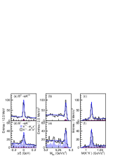
Figure 1: Distributions of the $\Delta E$, $M_{bc}$ and $M_{K^{+}K^{-}}$ for $B^{0}\to\phi K^{*0}$((a), (b) and (c)), and for $B^{+}\to\phi K^{*+}$((d), (e) and (f)), with other variables in signal region. Solid curves show the fit results. The continuum background components are shown by the dashed curves. The dark shaded areas represent the contributions from $B\to K^{+}K^{-}K^{*}$ and $B\to f_{0}K^{*}$ decays.

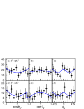
Figure 2: Projected distributions of the three transversity angles for $B^{0}\to\phi K^{*0}$((a), (b) and (c)), and for $B^{+}\to\phi K^{*+}$ ((d), (e) and (f)). Solid lines show the fit results. The points with error bars show the efficiency corrected data after background subtraction. The two $K^{*0}$ decay modes are combined in (d), (e) and (f). The discontinuity in (d) is due to the requirement of $\cos\theta_{K^{*}}$ in $B^{+}\to\phi K^{*+}(K^{*+}\to K^{+}\pi^{0})$.

Table 1: Number of events observed in the signal region($N_{ev}$) , signal yields ($N_{s}$), and the direct $CP$ asymmetries($A_{CP}$) obtained in the fits, with statistical and systematic uncertainties.

Mode	$N_{ev}$	$N_{s}$	$A_{CP}$
$\phi K^{*0}$	$309$	$173\pm 16$	$0.02\pm 0.09\pm 0.02$
$\phi K^{*+}$	$173$	$85^{+16}_{-11}$	$-0.02\pm 0.14\pm 0.03$
$\phi K^{*+}(K^{0}_{S}\pi^{+})$	$76$	$37.9^{+7.7}_{-7.0}$	$-0.14\pm 0.21\pm 0.04$
$\phi K^{*+}(K^{+}\pi^{0})$	$97$	$47.3^{+9.1}_{-8.1}$	$0.09\pm 0.19\pm 0.04$

Table 2: The decay amplitudes obtained for $B^{0}\to\phi K^{*0}$ and $B^{+}\to\phi K^{*+}$. the first uncertainties are statistical and the second are systematic.

$N_{ev}$	$\phi K^{*0}$	$\phi K^{*+}$
$|A_{0}|^{2}$	$0.45\pm 0.05\pm 0.02$	$0.52\pm 0.08\pm 0.03$
$|A_{\perp}|^{2}$	$0.30\pm 0.06\pm 0.02$	$0.19\pm 0.08\pm 0.02$
$\arg(A_{\parallel})$(rad)	$2.39\pm 0.24\pm 0.04$	$2.10\pm 0.28\pm 0.04$
$\arg(A_{\perp})$(rad)	$2.51\pm 0.23\pm 0.04$	$2.31\pm 0.30\pm 0.07$

Table 3: $\Lambda$ and $\Sigma$ values obtained from the decay amplitudes measured for $B^{0}$ and $\bar{B^{0}}$ separately.

	$B^{0}$	$\bar{B^{0}}$
$|A_{0}|^{2}$	$0.39\pm 0.08\pm 0.03$	$0.51\pm 0.07\pm 0.02$
$|A_{\perp}|^{2}$	$0.37\pm 0.09\pm 0.02$	$0.25\pm 0.07\pm 0.01$
$\arg(A_{\parallel})$(rad)	$2.72^{+0.46}_{-0.38}\pm 0.14$	$2.08\pm 0.31\pm 0.04$
$\arg(A_{\perp})$(rad)	$2.81\pm 0.36\pm 0.11$	$2.22\pm 0.35\pm 0.05$
$A^{0}_{T}$	$0.13^{+0.11}_{-0.14}\pm 0.04$	$0.28\pm 0.08\pm 0.01$
$A^{\parallel}_{T}$	$0.03\pm 0.08\pm 0.01$	$0.03\pm 0.06\pm 0.01$

Table 4: The measured decay amplitudes and triple-product correlations in the $B^{0}$ and $\bar{B^{0}}$ samples.

$\Lambda_{00}=0.45\pm 0.05\pm 0.02$	$\Sigma_{00}=-0.06\pm 0.05\pm 0.01$
$\Lambda_{\parallel\parallel}=0.24\pm 0.06\pm 0.02$	$\Sigma_{\parallel\parallel}=-0.01\pm 0.06\pm 0.01$
$\Lambda_{\perp\perp}=0.31\pm 0.06\pm 0.01$	$\Sigma_{\perp\perp}=-0.06\pm 0.05\pm 0.01$
$\Sigma_{\perp 0}=-0.41^{+0.16}_{-0.14}\pm 0.04$	$\Lambda_{\perp 0}=0.16^{+0.16}_{-0.14}\pm 0.03$
$\Sigma_{\perp\parallel}=-0.06\pm 0.10\pm 0.01$	$\Lambda_{\perp\parallel}=0.01\pm 0.10\pm 0.02$
$\Lambda_{\parallel 0}=-0.45\pm 0.11\pm 0.01$	$\Sigma_{\parallel 0}=-0.11\pm 0.11\pm 0.02$

The decay angles of a $B$-meson decaying to two vector mesons $\phi$ and $K^{*}$ are defined in the transversity basis$\!{}^{{\bf?}}$. The $x-y$ plane is defined to be the decay plane of $K^{*}$ and the $x$ axis is in the direction of the $\phi$ meson. The $y$ axis is perpendicular to the $x$ axis in the decay plane and is on the same side as the kaon from the $K^{*}$ decay. The $z$ axis is perpendicular to the $x-y$ plane according to the right-hand rule, $\theta_{\rm tr}(\phi_{\rm tr})$ is the polar(azimuthal) angle with respect to the $z$-axis of the $K^{+}$ from $\phi$ decay in the $\phi$ rest frame, and $\theta_{K^{*}}$ is defined earlier.

The distribution of the angles, $\theta_{K^{*}}$, $\theta_{\rm tr}$, and $\phi_{\rm tr}$ is given by$\!{}^{{\bf?}}$

$$\frac{d^{3}R_{\phi K^{*}}(\phi_{\rm tr},\cos\theta_{\rm tr},\cos\theta_{K^{*}})}{d\phi_{\rm tr}d\cos\theta_{\rm tr}d\cos\theta_{K^{*}}}=\frac{9}{32\pi}[|A_{\perp}|^{2}2\cos^{2}\theta_{\rm tr}\sin^{2}\theta_{K^{*}}+|A_{\parallel}|^{2}2\sin^{2}\theta_{\rm tr}\sin^{2}\phi_{\rm tr}\sin^{2}\theta_{K^{*}}$$

$$+|A_{0}|^{2}4\sin^{2}\theta_{\rm tr}\cos^{2}\phi_{\rm tr}\cos^{2}\theta_{K^{*}}+\sqrt{2}{\rm Re}(A_{\parallel}^{*}A_{0})\sin^{2}\theta_{\rm tr}\sin 2\phi_{\rm tr}\sin 2\theta_{K^{*}}$$

$$-\eta\sqrt{2}{\rm Im}(A_{0}^{*}A_{\perp})\sin 2\theta_{\rm tr}\cos\phi_{\rm tr}\sin 2\theta_{K^{*}}-2\eta{\rm Im}(A_{\parallel}^{*}A_{\perp})\sin 2\theta_{\rm tr}\sin\phi_{\rm tr}\sin^{2}\theta_{K^{*}}]$$

where $A_{0}$, $A_{\parallel}$, and $A_{\perp}$ are the complex amplitudes of the three helicity states in the transversity basis with the normalization condition $|A_{0}|^{2}+|A_{\parallel}|^{2}+|A_{\perp}|^{2}=1$, and $\eta==1(-1)$ corresponds to $B(\bar{B})$ mesons and is determined from the charge of the kaon or pion in the $K^{*}$ decay. The longitudinal polarization component is denoted by $A_{0}$ and $A_{\perp}(A_{\parallel})$ is the transverse polarization along the $z$-axis ($y$-axis). The value of $|A_{\perp}|$ $(|A_{0}|^{2}+|A_{\parallel}|^{2})$ is the $CP$-odd ($CP$-even) fraction in the decay $B\to\phi K^{*0}$ $\!{}^{{\bf?}}$. The presence of final state interactions (FSI) results in phases that differ from either $0$ or $\pm\pi$.

The complex amplitudes are determined by performing an unbinned maximum likelihood fit to the $B\to\phi K^{*}$ candidates in the signal region. The combined likelihood is given by

$$\mathcal{L}=\prod^{N_{ev}}_{i}\epsilon(\phi_{\rm tr},\cos\theta_{\rm tr},\cos\theta_{K^{*}})\sum_{j}f_{j}R_{j}(\phi_{\rm tr},\cos\theta_{\rm tr},\cos\theta_{K^{*}}),$$ (1)

where $j$ denotes the contributions from $\phi K^{*}$, $q\bar{q}$, $K^{+}K^{-}K^{*}$ and $f_{0}K^{*}$; $R_{j}$ is the angular distribution function (ADF). The ADF $R_{q\bar{q}}$ is determined from side-band data, and $R_{K^{+}K^{-}K^{*}}$ from events with $1.04{\rm GeV}/c^{2}<M_{K^{+}K^{-}}<1.075{\rm GeV}/c^{2}$; $R_{f_{0}K^{*}}$ is obtained from $B\to f_{0}K^{*}$ MC. The detection efficiency ($\epsilon$) is determined using MC simulations assuming a phase space decay. The fractions $f_{j}$ are parameterized as a function of $\Delta E$ $M_{bc}$ and $M_{K^{+}K^{-}}$. The value of $\arg(A_{0})$ is set to zero and $|A_{\parallel}|$ is calculated from the normalization condition. The four parameters ($|A_{0}|$, $|A_{\perp}|$, $\arg(A_{\parallel})$, and $\arg(A_{\perp})$) are determined from the fit. There is a two-fold ambiguity in the solutions for the phases; the chosen set of solutions is the one suggested in the reference $\!{}^{{\bf?}}$. Figure 2 shows the angular distributions with the projections of the fit superimposed. The obtained amplitudes are summarized in Table 2.

The systematic uncertainties on the amplitudes are dominated by the efficiency modeling (4-5%), continuum background (3-4%), slow pion efficiency (2-3%), and $K^{+}K^{-}K^{*}$ ADF (1-2%). The remaining possible systematic errors such as the angular resolution, signal yields, background from higher $K^{*}$ states, and width of the $f_{0}$ are estimated to be less than 1%.

The triple-product for a $B$ meson decay to two vector mesons takes the form $\vec{q}\cdot(\vec{\epsilon_{1}}\times\vec{\epsilon_{2}})$, where $\vec{q}$ is the momentum of one of the vector mesons, and $\vec{\epsilon_{1}}$ and $\vec{\epsilon_{2}}$ are the polarizations of the two vector mesons. The following two $T$-odd $\!{}^{{\bf?},{\bf?}}$ quantities

$$A^{0}_{T}={\rm Im}(A_{\perp}A^{*}_{0}),A^{\parallel}_{T}={\rm Im}(A_{\perp}A^{*}_{\parallel}),$$ (2)

provide information on the asymmetry of the triple products. The SM predicts very small values for $A^{0}_{T}$ and $A^{\parallel}_{T}$. The comparison of these triple product asymmetries ($A^{0}_{T}$ and $A^{\parallel}_{T}$) with the corresponding quantities for the $CP$-conjugated decays ($\bar{A}^{0}_{T}$ and $\bar{A}^{\parallel}_{T}$) provides an observable sensitive to $T$-violation.

Additional variables that can be measured through angular analysis are suggested$\!{}^{{\bf?}}$ and are given by

$$\Lambda_{\perp i}=-{\rm Im}(A_{\perp}A^{*}_{i}-\bar{A}_{\perp}\bar{A}^{*}_{i}), \Lambda_{\parallel 0}={\rm Re}(A_{\parallel}A^{*}_{0}+\bar{A}_{\parallel}\bar{A}^{*}_{0}),$$

$$\Sigma_{\perp i}=-{\rm Im}(A_{\perp}A^{*}_{i}+\bar{A}_{\perp}\bar{A}^{*}_{i}), \Sigma_{\parallel 0}={\rm Re}(A_{\parallel}A^{*}_{0}-\bar{A}_{\parallel}\bar{A}^{*}_{0}),$$

$$\Lambda_{\lambda\lambda}=\frac{1}{2}(|A_{\lambda}|^{2}+|\bar{A}_{\lambda}|^{2}), \Sigma_{\lambda\lambda}=\frac{1}{2}(|A_{\lambda}|^{2}-|\bar{A}_{\lambda}|^{2}),$$

where the subscript $\lambda$ is one of 0, $\parallel$, or $\perp$ and $i$ is one of 0 or $\parallel$. The variables $\Lambda_{\perp 0}$ and $\Lambda_{\perp\parallel}$ are sensitive to $T$-violating new physics. The following equations should hold in the absence of NP:

$$\Sigma_{\lambda\lambda}=0,\Sigma_{\parallel 0}=0,\Lambda_{\perp i}=0.$$

By separating $B^{0}$ and $\bar{B^{0}}$ samples and rearranging fitting parameters in the unbinned maximum likelihood fit, we obtain the decay amplitudes for the $B^{0}$ and $\bar{B^{0}}$, the triple-product correlations, and the other NP-sensitive observables, which are given in Table 3 and 4.

In summary improved measurements of the decay amplitudes $B\to\phi K^{*}$ are presented, based on fits to angular distributions in the transversity basis. The results are consistent with our previous measurements $\!{}^{{\bf?}}$ but with improved precision. The measured value of $|A_{\perp}|^{2}$ shows that $CP$-odd ($|A_{\perp}|^{2}$) and $CP$-even($|A_{0}|^{2}+|A_{\parallel}|^{2}$) components are present in $\phi K^{*}$ decays in a ratio of 1:2. Both phases of $A_{\perp}$ and $A_{\parallel}$ differ from zero or $-\pi$ rad by 4:3 standard deviations ($\sigma$) which provides evidence for the presence of final state interactions. The measured direct $CP$ asymmetries in these modes are consistent with zero. These correspond to 90% confidence level limits of $-0.14<A_{CP}(\phi K^{*0}(K^{+}\pi^{-}))<0.17$, and $-0.25<A_{CP}(\phi K^{*+})<0.22$. Difference between triple products asymmetries ($\Lambda_{\perp 0,\parallel}$) which are sensitive to $T$-violation are consistent with zero. The equations $\Sigma_{\lambda\lambda}=0$, $\Sigma_{\parallel 0}=0$, and $\Lambda_{\perp i}=0$ should be hold in the absence of NP. Our data does not show any significant violation of these relations. Measurements of the $T$-violation sensitive differences between triple product asymmetries, $A^{0}_{T}-\bar{A}^{0}_{T}$ and $A^{\parallel}_{T}-\bar{A}^{\parallel}_{T}$, indicate no significant deviations from zero. Our data indicates no significant deviations from the expectations: $\Sigma_{\lambda\lambda}=0$, $\Sigma_{\parallel 0}=0$, and $\Lambda_{\perp i}=0$, indicating no evidence for new physics.

3 $B\to\rho K^{*}$ Analysis

We select $B^{+}\to\rho^{+}K^{*0}$ candidate events by combining three charged tracks (two oppositely charged pions and on kaon) and one neutral pion. Each charged track is required to have a transverse momentum $p_{T}>0.1{\rm GeV}/c$ and be originated from the interaction point (IP). Candidates $\pi^{0}$ mesons are reconstructed from pairs of photons that have an invariant mass in the range $0.1178{\rm GeV}/c^{2}<M_{\pi^{0}}<0.1502{\rm GeV}/c^{2}$. The $\pi^{0}$ candidates are kinetically constrained to the nominal $\pi^{0}$ mass. In order to reduce the combinatorial background, we only accept $\pi^{0}$ candidates with momenta $p_{\pi^{0}}>0.40{\rm GeV}/c$ in the cms. Candidate $\rho^{+}$ mesons are reconstructed via their $\rho^{+}\to\pi^{+}\pi^{0}$ decay, and the $\pi^{+}\pi^{0}$ pairs are required to have an invariant mass in the region $0.62{\rm GeV}/c^{2}<M_{\pi^{+}\pi^{0}}<0.92{\rm GeV}/c^{2}$. Candidate $K^{*0}$ mesons are selected from the $K^{*0}\to K^{+}\pi^{-}$ decay with an invariant mass $0.83{\rm GeV}/c^{2}<M_{K^{+}\pi^{-}}<0.97{\rm GeV}/c^{2}$. To isolate the signal we accept events in the region $M_{bc}>5.2{\rm GeV}/c^{2}$ and $-0.3{\rm GeV}<\Delta E<0.3{\rm GeV}$, and define a signal region in $M_{bc}$ and $\Delta E$ as $M_{bc}>5.27{\rm GeV}/c^{2}$ and $-0.10{\rm GeV}<\Delta E<0.06{\rm GeV}$ respectively. The continuum process is the main source of background to be suppressed. In addition to the continuum process reduction at $B\to\phi K^{*}$ analysis, the displacement along the beam direction between the signal $B$ vertex and that of the other $B$, $\delta z$, also provides separation. For $B$ events, the average value of $\delta z$ is approximately $200\mu m$ while continuum events have a common vertex. This suppression removes 99.3% of the continuum background while retaining 41 % of the $B^{+}\to\rho^{+}K^{*0}$ events. The MC-determined efficiency with all selection criteria imposed is 2.7% for longitudinal polarization($A_{0}$) and 4.0% for transverse polarization ($A_{\pm}$).

To investigate backgrounds from $b\to c$ decays, we use a sample of $B\bar{B}$ MC events corresponding to an integrated luminosity of $412{\rm fb}^{-1}$. We find a contribution from $B^{+}\to\bar{D^{0}}(K^{+}\pi^{-}\pi^{0})\pi^{+}$ decays in the $\rho$ or $K^{*}$ sideband region and require$|M_{K\pi\pi^{0}}-M_{D^{0}}|>0.050{\rm GeV}/c^{2}$ to veto these events. Among the charmless $B$ decays, potential background arise from $B^{+}\to a_{1}^{0}K^{+}$, $B^{+}\to\rho^{+}K^{*0}(1430)$, non-resonant $B^{+}\to\rho^{+}K^{+}\pi^{-}$ and $B^{+}\to K^{*0}\pi^{+}\pi^{0}$. We separate signal from these backgrounds by fitting the $\rho$ and $K^{*}$ invariant mass distributions.

We extract the signal yield by applying an extended unbinned maximum-likelihood fit to the two-dimensional $M_{bc}-\Delta E$ distribution. The fit includes components for signal plus backgrounds from continuum events and $b\to c$ decays. The PDFs for signal and $b\to c$ decay are modeled by smoothed two-dimensional histograms obtained from large MC samples. The signal PDF is adjusted to account for small differences observed between data and MC for a high-statistics mode containing $\pi^{0}$ mesons, $B^{+}\to\bar{D^{0}}(K^{+}\pi^{-}\pi^{0})\pi^{+}$. The continuum PDF is described by a product of a threshold (ARGUS) function for $M_{bc}$ and a first-order polynomial for $\Delta E$, with shape parameters allowed to vary. All normalizations are allowed to float. Figure 4 shows the final event sample and the fit results. The five-parameter (three normalizations plus two shape parameters for continuum) fit yields $134.8\pm 16.9$ $B^{+}\to K^{+}\pi^{-}\pi^{+}\pi^{0}$ events.

Figure 3: Projections of $M_{bc}$ for events in the $\Delta E$ signal region (left), and projection of $\Delta E$ in the $M_{bc}$ signal region (right). The solid curves show the results of the fit. The hatched histograms represent the continuum background. The sum of the $b\to c$ and continuum background component is shown as dot-dashed lines.

Figure 4: Signal yields obtained from the $M_{bc}-\Delta E$ distribution in bins of $M_{\pi^{+}\pi^{0}}$ (left) for events in the $K^{*0}$ region and in bins of $M_{K\pi}$ (right) for events in the $\rho$ region. Solid curves show the results of the fit. Hatched histograms are for the non-resonant component.

We further distinguish the $\rho^{+}K^{*0}$ signal from non-resonant decays such as $B^{+}\to\rho^{+}K^{+}\pi^{-}$ or $B^{+}\to K^{*0}\pi^{+}\pi^{0}$ by fitting the $M_{\pi^{+}\pi^{0}}$ and $M_{K\pi}$ invariant mass distributions. The signal yields obtained from the $M_{bc}-\Delta E$ fit for different $M_{\pi^{+}\pi^{0}}$ and $M_{K\pi}$ bins are plotted in Figure 4, where the $M_{\pi^{+}\pi^{0}}$ distribution is for events in the $K^{*0}$ region ($0.83{\rm GeV}/c^{2}<M_{K\pi}<0.97{\rm GeV}/c^{2}$) and the the $M_{K\pi}$ distribution is for events in the $\rho$ region ($0.62{\rm GeV}/c^{2}<M_{\pi^{+}\pi^{0}}<0.92{\rm GeV}/c^{2}$). We perform separate $\chi^{2}$ fits to the $M_{\pi\pi}$ or $M_{K\pi}$ distributions. Each fit includes components for signal and non-resonant background. the signal $\rho$ and $K^{*}$ PDFs are modeled by relativistic $P$-wave Breit-Wigner functions with means and widths fixed at their known values $\!{}^{{\bf?}}$; the PDFs are convolved with a Gaussian of $\sigma=5.3{\rm MeV}$, which is obtained by fitting the $D^{0}(K^{-}\pi^{+})$ invariant mass, to account for the detector resolution. The non-resonant component is represented by a threshold function with parameters determined from MC events where the final states are distributed uniformly over phase space. The $M_{\pi\pi}$ mass fit gives $125.4\pm 15.8\rho$ and $-0.3\pm 3.0$ non-resonant events in the $K^{*}$ mass region. The statistical significance of the signal, defined as $\sqrt{\chi^{2}_{0}-\chi^{2}_{min}}$, where $\chi^{2}_{min}$ is the $\chi^{2}$ value at the best-fit signal yield and $\chi^{2}_{0}$ is the value with the $K^{*0}$ signal yield set to zero, is $5.3\sigma$($5.2\sigma$ with the inclusion of systematics). The contribution from non-resonant $\rho^{+}K^{+}\pi^{-}$ is significant and is taken into account in both the branching fraction and polarization determinations, while we neglect the non-resonant $K^{*0}\pi^{+}\pi^{0}$ contribution.

We use the $\rho^{+}\to\pi^{+}\pi^{0}$ and $K^{*0}\to K^{+}\pi^{-}$ helicity-angle ($\theta_{\rho},\theta_{K^{*}}$) distributions to determine the relative strengths of $|A_{0}|^{2}$ and $|A_{\pm}|^{2}$. Here $\theta_{\rho}(\theta_{K^{*}})$ is the angle between an axis anti-parallel to the $B$ flight direction and the $\pi^{+}(K^{+})$ flight direction in the $\rho(K^{*})$ rest frame. For the longitudinal polarization case, the distribution is proportional to $\cos^{2}\theta_{\rho}\cos^{2}\theta_{K^{*}}$, and for the transverse polarization case, it is proportional to $\sin^{2}\theta_{\rho}\sin^{2}\theta_{K^{*}}$ $\!{}^{{\bf?}}$. Figure 5 shows the signal yields obtained from $M_{bc}-\Delta E$ fits in bins of the cosine of the helicity angle for $\rho$ and $K^{*}$. We perform a binned simultaneous $\chi^{2}$ fit to the $\rho$ and $K^{*}$ helicity-angle distributions. The fit includes components for signal and non-resonant $\rho K\pi$. PDFs for signal $A_{0}$ and $A_{\pm}$ helicity states are determined from the MC simulation. The helicity-angle distribution for data in the high $M_{K\pi}$ sideband region $1.1{\rm GeV}/c^{2}<M_{K\pi}<1.5{\rm GeV}/c^{2}$, where $\rho K\pi$ events dominate, is consistent with a $\cos^{2}\theta$-like $\cos\theta_{\rho}$ and a flat $\cos\theta_{K^{*}}$ distribution. Thus, we assume an $S$-wave $K\pi$ system and model the non-resonant $B\to\rho K\pi$ PDF based on the MC simulation. The fraction of the non-resonant component is fixed at the values obtained from the $K^{*}$ mass fit. The two parameter (normalizations for $A_{0}$ and $A_{\pm}$) fit result deviates from 100% longitudinal polarization with a significance of $4.9\sigma$ ($4.3\sigma$ including systematic uncertainties). The significance is defined as $\sqrt{\chi^{2}_{0}-\chi^{2}_{\rm min}}$, where $\chi^{2}_{\rm min}$ is the $\chi^{2}$ value at the best-fit and $\chi^{2}_{0}$ is the value with the longitudinal polarization fraction set to 100%.

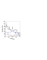
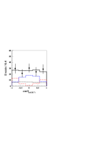
Figure 5: Fit to background-subtracted helicity distributions. The solid histograms show the results. The dot-dashed (dashed) histograms are the $A_{0}(A_{\pm})$ component of the fit; the dotted histograms are for non-resonant $\rho K\pi$. The low event near $\cos\theta_{\rho}=1$ is due to the $p_{\pi^{0}}>0.4{\rm GeV}/c$ requirement.

The largest uncertainties in the polarization measurement are due to uncertainties in the non-resonant $\rho K\pi$ PDF, potential scalar-pseudoscalar ($S-P$) interference, and the non-resonant fraction. We assign ${}^{+10.3}_{-0}\%$ systematic error for the non-resonant PDF. This uncertainty is estimated by adding a $1/3$ flat component to the $\rho$ helicity PDF for non-resonant $\rho K\pi$ in the helicity fit. Interference of the longitudinal amplitude $A_{0}$ with the $S$-wave ($K\pi$) system introduces a term with a $2e^{i\Delta\phi}|A_{\rho K\pi}|\cos\theta_{K^{*}}$ dependence, where $\Delta\phi$ is the phase difference and $|A_{\rho K\pi}|$ is amplitude of the $B\to\rho K\pi$ decay. The $S-P$ wave interference disappears in the $\cos\theta_{\rho}$ distribution, which is integrated over $\cos\theta_{K^{*}}$; however it remains in the $\cos\theta_{K^{*}}$ distribution. We include an additional linear function for the interference term in the $\cos\theta_{K^{*}}$ helicity and redo the $\chi^{2}$ fit. The resulting small change in $f_{L}$, 0.5%, is assigned as the systematic uncertainty for the $S-P$ interference. A ${}^{+4.0}_{-4.1}\%$ systematic error is assigned for the uncertainty in the fraction of non-resonant $\rho K\pi$, obtained by varying the non-resonant fraction by $\pm 1\sigma$. Adding the various systematic error contributions in quadrature, we obtain the longitudinal polarization fraction in $B^{+}\to\rho^{+}K^{*0}$ decays,

$$f_{L}(B^{+}\to\rho^{+}K^{*0})=0.43\pm 0.11({\rm stat.})^{+0.05}_{-0.02}({\rm syst.}).$$

To calculate the $B^{+}\to\rho^{+}K^{*0}$ branching fraction, we use the invariant mass fit result and MC-determined efficiencies weighted by the measured polarization components. We consider systematic errors in the branching fraction that are caused by uncertainties in the efficiencies of track finding, particle identification, $\pi^{0}$ reconstruction, continuum suppression, fitting, polarization fraction. We assign an error of 1.1% per track for the uncertainty in the track efficiency. This uncertainty is obtained from a study of partially reconstructed $D^{*}$ decays. We also assign an uncertainty of 0.7% per track on the particle identification efficiency, based on a study of kinematically selected $D^{*+}\to D^{0}(K^{-}\pi^{+})\pi^{+}$ decay. A 4.0% systematic error for the uncertainty in the $\pi^{0}$ detection efficiency is determined from data-MC comparisons of $\eta\to\pi^{0}\pi^{0}\pi^{0}$ with $\eta\to\pi^{+}\pi^{-}\pi^{0}$ and $\eta\to\gamma\gamma$. A 4.5% systematic error for continuum suppression is estimated from studying the process $B^{+}\to\bar{D^{0}}(K^{+}\pi^{-}\pi^{0})\pi^{+}$. A -4.2%/+1.7% error due to the uncertainty in the fraction of longitudinal polarization is obtained by varying $f_{L}$ by its errors. The uncertainty in non-resonant $K^{*}\pi\pi$ background gives a contribution of -2.2%/+0% in addition to -3.0%/+2.3% error from uncertainties in the background from other rare $B$ decays. A 1.1% error for the uncertainty in the number of $B\bar{B}$ events in the data sample. A 7.1% error for possible bias in the $\chi^{2}$ fit $\!{}^{{\bf?}}$, obtained from a MC study is also included. The quadratic sum of all of these errors is taken as the total systematic error. We obtain the branching fraction

$$\mathcal{B}(B^{+}\to\rho^{+}K^{*0})=(8.9\pm 1.7({\rm stat})\pm 1.2({\rm syst})\times 10^{-6}.$$

In summary, we have observed the $B^{+}\to\rho^{+}K^{*0}$ decay with a statistical significance of $5.3\sigma$. We measure the branching fraction to be $(8.9\pm 1.7({\rm stat})\pm 1.2({\rm syst})\times 10^{-6}$. We also perform a helicity analysis and find a substantial transversely polarized fraction with a statistical significance of $4.9\sigma$. The longitudinal polarization fraction $f_{L}$ measured is similar to the surprisingly low value found in $b\to s\bar{s}s$ decays $B\to\phi K^{*}$.

References

References

- [1] A. L. Kagan, Phys. Lett. B 601, 151 (2004).
- [2] Belle Collaboration, J. Zhang et al, Phys. Rev. Lett. 91, 221801 (2003).
- [3] BaBar Collaboration, B. Aubert et al, Phys. Rev. Lett. 93, 231801 (2004).
- [4] BaBar Collaboration, B. Aubert et al, Phys. Rev. Lett. 91, 171802 (2003).
- [5] BaBar Collaboration, B. Aubert et al, Phys. Rev. Lett. 93, 231804 (2004).
- [6] Belle Collaboration, K.-F. Chen et al, Phys. Rev. Lett. 91, 201801 (2003).
- [7] H-n Li, hep-ph/0411305 (2004).
- [8] Y. Grossman, Int. J. Mod. Phys. A 19, 907(2004).
- [9] Y. D Yang, R. M Wang, G. R Lu, hep-ph/0411211 (2004).
- [10] Belle Collaboration, A. Abashian et al., Nucl. Instr. and Meth. A 479, 117 (2002).
- [11] S. Kurokawa and E. Kikutani, Nucl. Instrum. Meth., A499, 1 (2003), and other papers included in this Volume.
- [12] CLEO Collaboration, R. Ammar et al, Phys. Rev. Lett. 71, 674 (1993).
- [13] Belle Collaboration, K. Abe et al, Phys. Lett. B 517, 309 (2001).
- [14] H. Kakuno et al, Nucl. Instrum. Methods A 499, 1 (2003).
- [15] A. Garmash et al, hep-ex/0412066.
- [16] S.Eidelman et al, Phys. Lett. B 592, 1 (2004).
- [17] ARGUS Collaboration, H. Albrecht et al, Phys. Lett. B 241, 278 (1990); 254, 288 (1991).
- [18] I. Dunietz et al, Phys. Rev. D 43, 2193 (1991).
- [19] K. Abe, M. Satpathy and H. Yamamoto, hep-ex/0103002.
- [20] M. Suzuki, Phys. Rev. D 64, 117503 (2001).
- [21] A. Datta and D. London, Int. J. Mod. Phys. A 19, 2505(2004).
- [22] D. London, N. Sinha and R. Sinha, Phys. Rev. D 69, 114013 (2004).
- [23] Definisions are , and , but , and .
- [24] S. Baker, R. D. Cousins, Nucl. Instrum. Methods A 221, 437 (1984).