Abstract

Polarized antiprotons, produced by spin filtering with an internal polarized gas target, provide access to a wealth of single– and double–spin observables, thereby opening a new window to physics uniquely accessible at the HESR. This includes a first measurement of the transversity distribution of the valence quarks in the proton, a test of the predicted opposite sign of the Sivers–function, related to the quark distribution inside a transversely polarized nucleon, in Drell–Yan (DY) as compared to semi–inclusive DIS, and a first measurement of the moduli and the relative phase of the time–like electric and magnetic form factors $G_{E,M}$ of the proton. In polarized and unpolarized $p\bar{p}$ elastic scattering, open questions like the contribution from the odd charge–symmetry Landshoff–mechanism at large $|t|$ and spin–effects in the extraction of the forward scattering amplitude at low $|t|$ can be addressed. The proposed detector consists of a large–angle apparatus optimized for the detection of DY electron pairs and a forward dipole spectrometer with excellent particle identification.

The design and performance of the new components, required for the polarized antiproton program, are outlined. A low–energy Antiproton Polarizer Ring (APR) yields an antiproton beam polarization of $P_{\bar{p}}$ = 0.3 to 0.4 after about two beam life times, which is of the order of 5–10 h. By using an internal $\rm H^{\uparrow}$ target and a detector installed in a 3.5 GeV/c Cooler Synchrotron Ring (CSR), the Phase–I experimental $\bar{p}^{\uparrow}p^{\uparrow}$ program could start in 2014, completely independent of the operation of the HESR. In Phase–II, the CSR serves as an injector for the polarized antiprotons into the HESR. A chicane system inside the HESR is proposed to guide the high–energy $\bar{p}^{\uparrow}$ beam to the PAX detector, located inside the CSR straight section. In Phase–II, fixed–target or collider $\bar{p}^{\uparrow}p^{\uparrow}$ experiments over a broad energy range become possible. In the collider mode, polarized protons stored in the CSR up to momenta of 3.5 GeV/c are bombarded head–on with 15 GeV/c polarized antiprotons stored in the HESR. This asymmetric double–polarized antiproton–proton collider is ideally suited to map e.g. the transversity distribution in the proton.

The appendices contained in this document were composed only after the main document had been submitted to the QCD-PAC. Appendix A discusses the polarization–transfer technique that PAX will exploit to produce a beam of polarized antiprotons, and applications of this technique in the high–energy sector. The spin–dependence of the antiproton–proton interaction and the special interest in double–polarized antiproton-proton scattering at very low energies, in view of the indications for the protonium state, is elaborated in Appendix B. In Appendix C, we discuss details of the impact of recent data from electron–positron collider experiments on the proton–antiproton physics, accessible in Phase I of the PAX experimental program. A comment on the Next-to-Leading-Order corrections to the Drell-Yan process is presented in Appendix D. Appendix E describes beam dynamics simulations that have been carried out recently for the proton–antiproton collider mode of the PAX experiment making use of the CSR and the HESR. Based on conservative assumptions about the number of antiprotons accumulated in the HESR, these calculations indicate that a luminosity of about ${\cal L}=1.5\times 10^{30}$ cm^-2s^-1 can be achieved in the PAX collider mode. An extensive program of Monte Carlo studies, described in Appendix F, has been started to investigate different options for the PAX detector configuration, aiming at an optimization of the achievable performance.

Members of the Collaboration

Alessandria, Italy, Universita^′ del Piemonte Orientale ^′′A. Avogadro^′′ and INFN

Vincenzo Barone

Beijing, China, School of Physics, Peking University

Bo–Qiang Ma

Bochum, Germany, Institut für Theoretische Physik II, Ruhr Universität Bochum

Klaus Goeke, Andreas Metz, and Peter Schweitzer

Bonn, Germany, Helmholtz–Institut für Strahlen– und Kernphysik, Universität Bonn

Jens Bisplinghoff, Paul–Dieter Eversheim, Frank Hinterberger, Ulf–G. Meißner, Heiko Rohdjeß, and Alexander Sibirtsev

Brookhaven, USA, Collider–Accelerator Department, Brookhaven National Laboratory

Christoph Montag

Brookhaven, USA, RIKEN BNL Research Center, Brookhaven National Laboratory

Werner Vogelsang

Cagliari, Italy, Dipartimento di Fisica, Universita^′ di Cagliari and INFN

Umberto D^′Alesio, and Francesco Murgia

Dublin, Ireland, School of Mathematics, Trinity College, University of Dublin

Nigel Buttimore

Dubna, Russia, Bogoliubov Laboratory of Theoretical Physics, Joint Institute for Nuclear Research

Anatoly Efremov, and Oleg Teryaev

Dubna, Russia, Dzhelepov Laboratory of Nuclear Problems, Joint Institute for Nuclear Research

Sergey Dymov, Natela Kadagidze, Vladimir Komarov, Anatoly Kulikov, Vladimir Kurbatov, Vladimir Leontiev, Gogi Macharashvili, Sergey Merzliakov, Igor Meshkov, Valeri Serdjuk, Anatoly Sidorin, Alexander Smirnow, Evgeny Syresin, Sergey Trusov, Yuri Uzikov, Alexander Volkov, and Nikolai Zhuravlev

Dubna, Russia, Laboratory of Particle Physics, Joint Institute for Nuclear Research

Oleg Ivanov, Victor Krivokhizhin, Gleb Meshcheryakov, Alexander Nagaytsev, Vladimir Peshekhonov, Igor Savin, Binur Shaikhatdenov, Oleg Shevchenko, and Gennady Yarygin

Erlangen, Germany, Physikalisches Institut, Universität Erlangen–Nürnberg

Wolfgang Eyrich, Andro Kacharava, Bernhard Krauss, Albert Lehmann, Davide Reggiani, Klaus Rith, Ralf Seidel, Erhard Steffens, Friedrich Stinzing, Phil Tait, and Sergey Yaschenko

Ferrara, Italy, Istituto Nazionale di Fisica Nucleare

Marco Capiluppi, Guiseppe Ciullo, Marco Contalbrigo, Alessandro Drago, Paola Ferretti–Dalpiaz, Francesca Giordano, Paolo Lenisa, Luciano Pappalardo, Giulio Stancari, Michelle Stancari, and Marco Statera

Frascati, Italy, Istituto Nazionale di Fisica Nucleare

Eduard Avetisyan, Nicola Bianchi, Enzo De Sanctis, Pasquale Di Nezza, Alessandra Fantoni, Cynthia Hadjidakis, Delia Hasch, Marco Mirazita, Valeria Muccifora, Federico Ronchetti, and Patrizia Rossi

Gatchina, Russia, Petersburg Nuclear Physics Institute

Sergey Barsov, Stanislav Belostotski, Oleg Grebenyuk, Kirill Grigoriev, Anton Izotov, Anton Jgoun, Peter Kravtsov, Sergey Manaenkov, Maxim Mikirtytchiants, Sergey Mikirtytchiants, Oleg Miklukho, Yuri Naryshkin, Alexander Vassiliev, and Andrey Zhdanov

Gent, Belgium, Department of Subatomic and Radiation Physics, University of Gent

Dirk Ryckbosch

Hefei, China, Department of Modern Physics, University of Science and Technology of China

Yi Jiang, Hai–jiang Lu, Wen–gan Ma, Ji Shen, Yun–xiu Ye, Ze–Jie Yin, and Yong–min Zhang

Jülich, Germany, Forschungszentrum Jülich, Institut für Kernphysik

David Chiladze, Ralf Gebel, Ralf Engels, Olaf Felden, Johann Haidenbauer, Christoph Hanhart, Michael Hartmann, Irakli Keshelashvili, Siegfried Krewald, Andreas Lehrach, Bernd Lorentz, Sigfried Martin, Ulf–G. Meißner, Nikolai Nikolaev, Dieter Prasuhn, Frank Rathmann, Ralf Schleichert, Hellmut Seyfarth, and Hans Ströher

Kosice, Slovakia, Institute of Experimental Physics, Slovak Academy of Sciences and P.J. Safarik University, Faculty of Science

Dusan Bruncko, Jozef Ferencei, Ján Mušinský, and Jozef Urbán

Langenbernsdorf, Germany, Unternehmensberatung und Service–Büro (USB), Gerlinde Schulteis & Partner GbR

Christian Wiedner (formerly at MPI-K Heidelberg)

Lecce, Italy, Dipartimento di Fisica, Universita^′ di Lecce and INFN

Claudio Corianó, and Marco Guzzi

Madison, USA, University of Wisconsin

Tom Wise

Milano, Italy, Universita’ dell’Insubria, Como and INFN sez.

Philip Ratcliffe

Moscow, Russia, Institute for Theoretical and Experimental Physics

Vadim Baru, Ashot Gasparyan, Vera Grishina, Leonid Kondratyuk, and Alexander Kudriavtsev

Moscow, Russia, Lebedev Physical Institute

Alexander Bagulya, Evgeni Devitsin, Valentin Kozlov, Adel Terkulov, and Mikhail Zavertiaev

Moscow, Russia, Physics Department, Moscow Engineering Physics Institute

Aleksei Bogdanov, Sandibek Nurushev, Vitalii Okorokov, Mikhail Runtzo, and Mikhail Strikhanov

Novosibirsk, Russia, Budker Institute for Nuclear Physics

Yuri Shatunov

Palaiseau, France, Centre de Physique Theorique, Ecole Polytechnique

Bernard Pire

Protvino, Russia, Institute of High Energy Physics

Nikolai Belikov, Boris Chujko, Yuri Kharlov, Vladislav Korotkov, Viktor Medvedev, Anatoli Mysnik, Aleksey Prudkoglyad, Pavel Semenov, Sergey Troshin, and Mikhail Ukhanov

Tbilisi, Georgia, Institute of High Energy Physics and Informatization, Tbilisi State University

Badri Chiladze, Nodar Lomidze, Alexander Machavariani, Mikheil Nioradze, Tariel Sakhelashvili, Mirian Tabidze, and Igor Trekov

Tbilisi, Georgia, Nuclear Physics Department, Tbilisi State University

Leri Kurdadze, and George Tsirekidze

Torino, Italy, Dipartimento di Fisica Teorica, Universita di Torino and INFN

Mauro Anselmino, Mariaelena Boglione, and Alexei Prokudin

Uppsala, Sweden, Department of Radiation Sciences, Nuclear Physics Division

Pia Thorngren–Engblom

Virginia, USA, Department of Physics, University of Virginia

Simonetta Liuti

Warsaw, Poland, Soltan Institute for Nuclear Studies

Witold Augustyniak, Bohdan Marianski, Lech Szymanowski, Andrzej Trzcinski, and Pawel Zupranski

Yerevan, Armenia, Yerevan Physics Institute

Norayr Akopov, Robert Avagyan, Albert Avetisyan, Garry Elbakyan, Zaven Hakopov, Hrachya Marukyan, and Sargis Taroian

Spokespersons:

Paolo Lenisa, E–Mail: lenisa@mail.desy.de
Frank Rathmann, E–Mail: f.rathmann@fz–juelich.de

Contents

1. I Physics Case
   1. 1 Preface
   2. 2 Accessing Transversity Distributions
      1. 2.1 Spin Observables and Transversity
      2. 2.2 Transversity in Drell–Yan Processes at PAX
      3. 2.3 Transversity in $D$–Meson Production at PAX
   3. 3 Single Spin Asymmetries and Sivers Function
   4. 4 Electromagnetic Form Factors of the Proton
   5. 5 Hard Scattering: Polarized and Unpolarized
   6. 6 Polarized Antiproton–Proton Soft Scattering
      1. 6.1 Low–$t$ Physics
      2. 6.2 Total Cross Section Measurement
      3. 6.3 Proton–Antiproton Interaction
2. II Polarized Antiprotons at FAIR
   1. 7 Overview
   2. 8 Antiproton Polarizer Ring
      1. 8.1 The Polarizing Process $\bar{p}+\vec{e}\to\vec{\bar{p}}+e$
      2. 8.2 Design Consideration for the APR
         1. 8.2.1 Polarizer Target
         2. 8.2.2 Beam Lifetime in the APR
      3. 8.3 Polarization Buildup
         1. 8.3.1 Space–Charge Limitations
         2. 8.3.2 Optimum Beam Energies for the Polarization Buildup
         3. 8.3.3 Polarized Targets containing only Electrons
      4. 8.4 Luminosity Estimate for a Fixed Target in the HESR
      5. 8.5 Technical Realization of the APR
         1. 8.5.1 Constraints
         2. 8.5.2 Layout of the APR Lattice
         3. 8.5.3 Features of the APR Design
         4. 8.5.4 Discussion of the APR Design
         5. 8.5.5 Realization of the APR based on Permanent Magnets
   3. 9 Cooler Synchrotron Ring CSR
      1. 9.1 Injector LINAC for 50 MeV Polarized Protons
      2. 9.2 Acceleration of Polarized Proton and Antiproton Beam
         1. 9.2.1 Imperfection Resonances
         2. 9.2.2 Intrinsic Resonances
   4. 10 PAX Requirements on the HESR Design
      1. 10.1 Introduction
      2. 10.2 Polarization Preservation
         1. 10.2.1 Depolarizing Resonances
         2. 10.2.2 Siberian Snake with Combined Fields
         3. 10.2.3 Siberian Snake with Solenoidal Fields
      3. 10.3 Spin Manipulation of Polarized Protons and Antiprotons
      4. 10.4 Interaction Region Design for the Asymmetric Collider
         1. 10.4.1 Luminosity Estimate for the Asymmetric Collider
         2. 10.4.2 Intensity dependent Limitations
            1. 10.4.2.1 Touschek Lifetime
            2. 10.4.2.2 Intrabeam Scattering
   5. 11 Polarimetry
3. III Staging of Experiments
   1. 12 Preparatory Phase
      1. 12.1 Accelerator: Design and Construction of the Antiproton Polarizer Ring
      2. 12.2 Physics in the Preparatory Phase
      3. 12.3 Development of Polarized Sources
   2. 13 Phase–I
      1. 13.1 Accelerator: Transfer of APR and CSR to FAIR
      2. 13.2 Physics in Phase–I
   3. 14 Phase–II
      1. 14.1 Accelerator: HESR modifications to collider mode or to polarized internal target.
      2. 14.2 Physics in Phase–II
4. IV Detector
   1. 15 Requirements and Design Considerations
      1. 15.1 Physical Channels
      2. 15.2 Particle Identification
      3. 15.3 Magnetic Field Configuration
      4. 15.4 Mass Resolution
      5. 15.5 General Remarks
   2. 16 Overview of the PAX Spectrometer
      1. 16.1 Toroid Magnet
      2. 16.2 Silicon Detector
      3. 16.3 Drift Chambers
      4. 16.4 Čerenkov Detector
      5. 16.5 Calorimeter
      6. 16.6 Hodoscopes
      7. 16.7 Forward Spectrometer
      8. 16.8 Recoil Detector
      9. 16.9 Trigger and Data Acquisition
   3. 17 Detector Phases
      1. 17.1 Detector Phase–I
         1. 17.1.1 The gaseous Fixed-Target
         2. 17.1.2 The Target Magnet
      2. 17.2 Detector Phase–II
   4. 18 Performance Summary
   5. 19 Alternative Scenarios
      1. 19.1 Drell–Yan with Muons
      2. 19.2 Solenoid Magnet
5. V Organization
   1. 20 Logistics of the Experiment
      1. 20.1 Floor Space
      2. 20.2 Radiation Environment
      3. 20.3 Responsibilities and Manpower
         1. 20.3.1 Institutional Responsibilities (preliminary list)
         2. 20.3.2 Manpower
      4. 20.4 Schedule
         1. 20.4.1 Milestones
         2. 20.4.2 Timelines
      5. 20.5 Cost Estimates
6. VI Appendix A
   1. A Polarization Transfer Technique & Applications
      1. A.1 Breit Hamiltonian and Antiproton Polarizer
      2. A.2 Polarized Electron–Proton Elastic Scattering: Theory
      3. A.3 Beam–target Double–spin Asymmetry and $G_{E}/G_{M}$
      4. A.4 Electron Proton Polarization Transfer and $G_{E}$/$G_{M}$: Theory
      5. A.5 Electron Proton Polarization Transfer: Experiment
      6. A.6 Electron–to–Neutron Polarization Transfer and $G_{E}^{n}/G_{M}^{n}$: Experiment
      7. A.7 Summary
7. VII Appendix B
   1. B Polarized Antiproton-Proton Soft Scattering
      1. B.1 Spin effects in the Interpretation of Coulomb–Nuclear Interference
      2. B.2 Separation of Spin–Singlet and Spin–Triplet Scattering at Low Energy
      3. B.3 The Impact of the Spin–Dependence of Antiproton–Proton Scattering on the Polarization Buildup
      4. B.4 Summary
8. VIII Appendix C
   1. C Resonance Structures and Phase Motion of the Electromagnetic Form Factors in the Time-like Region
      1. C.1 Resonance Structures and Nuclear Baryonium States in $N\bar{N}$ Interactions
      2. C.2 $N\bar{N}$ Interaction and the Interpretation of the BES Results
      3. C.3 Summary: Baryonium and $N\bar{N}$ Resonances in $p\bar{p}\to e^{+}e^{-}$
9. IX Appendix D
   1. D Comments on Drell-Yan Cross Sections and Spin Asymmetries in the PAX Kinematic Regime
      1. D.1 Factorization and Perturbation Theory for the Drell-Yan Process
      2. D.2 Phenomenological Studies in the PAX Kinematic Regimes
      3. D.3 Resummations and Nonperturbative Power Corrections
      4. D.4 Conclusions
10. X Appendix E
    1. E Beam Dynamics Simulations for the PAX using the BETACOOL code
       1. E.1 Introduction
       2. E.2 The Cooling Process
       3. E.3 Cycling of APR, CSR and HESR
       4. E.4 Possible Improvements
       5. E.5 Summary
11. XI Appendix F
    1. F Detector Simulation for PAX
       1. F.1 PAX detector concept
       2. F.2 Phase–I: Electromagnetic form factors of the proton and hard elastic scattering
          1. F.2.1 Electromagnetic form factors of the proton
       3. F.3 Hard elastic scattering
       4. F.4 Phase–II: The transversity measurement
          1. F.4.1 Detector Simulation
          2. F.4.2 Background Evaluation
          3. F.4.3 Detector Performance
       5. F.5 Summary
          1. F.5.1 Phase-I
          2. F.5.2 Phase–II

Part I Physics Case

1 Preface

The polarized antiproton–proton interactions at HESR will allow a unique access to a number of new fundamental physics observables, which can be studied neither at other facilities nor at HESR without transverse polarization of protons and/or antiprotons:

• The transversity distribution is the last leading–twist missing piece of the QCD description of the partonic structure of the nucleon. It describes the quark transverse polarization inside a transversely polarized proton [1]. Unlike the more conventional unpolarized quark distribution $q(x,Q^{2})$ and the helicity distribution $\Delta q(x,Q^{2})$, the transversity $h^{q}_{1}(x,Q^{2})$ can neither be accessed in deep–inelastic scattering of leptons off nucleons nor can it be reconstructed from the knowledge of $q(x,Q^{2})$ and $\Delta q(x,Q^{2})$. It may contribute to some single–spin observables, but always coupled to other unknown functions. The transversity distribution is directly accessible uniquely via the double transverse spin asymmetry $A_{TT}$ in the Drell–Yan production of lepton pairs. The theoretical expectations for $A_{TT}$ in the Drell–Yan process with transversely polarized antiprotons interacting with a transversely polarized proton target or beam at HESR are in the 30–40 per cent range [2, 3]; with the expected antiproton spin–filtering rate and luminosity of HESR the PAX experiment is uniquely suited for the definitive observation of $h^{q}_{1}(x,Q^{2})$ of the proton for the valence quarks.

• The PAX measurements can also provide completely new insights into the understanding of (transverse) single–spin asymmetries (SSA) which have been observed in proton–proton and proton–antiproton collisions as well as in lepton–nucleon scattering. For instance through charm production ($\bar{p}^{\uparrow}\,p\to D\,X$ or $\bar{p}\,p^{\uparrow}\to D\,X$) it will be possible to disentangle the Sivers [4] and the Collins mechanisms [5]. In general, both effects contribute to the measured SSA (mostly in $p^{\uparrow}\,p\to\pi\,X$ and $\bar{p}^{\uparrow}\,p\to\pi\,X$ ), but in the case of charm production the Collins mechanism drops out. Moreover, in conjunction with the data on SSA from the HERMES collaboration [6, 7], the PAX measurements of the SSA in Drell–Yan production on transversely polarized protons can for the first time provide a test of the theoretical prediction [8] of the sign–reversal of the Sivers function from semi–inclusive DIS to Drell–Yan processes. Both studies will crucially test and improve our present QCD–description of the intriguing phenomenon of SSA.

• The origin of the unexpected $Q^{2}$–dependence of the ratio of the magnetic and electric form factors of the proton, as observed at the Jefferson laboratory [9], can be clarified by a measurement of their relative phase in the time–like region, which discriminates strongly between the models for the form factor. This phase can be measured via SSA in the annihilation $\bar{p}p^{\uparrow}\to e^{+}e^{-}$ on a transversely polarized target [10, 11]. The first ever measurement of this phase at PAX will also contribute to the understanding of the onset of the pQCD asymptotics in the time–like region and will serve as a stringent test of dispersion theory approaches to the relationship between the space–like and time–like form factors [12, 13, 14]. The double–spin asymmetry will fix the relative phase ambiguity and allow independently the $G_{E}-G_{M}$ separation, which will serve as a check of the Rosenbluth separation in the time–like region.

• Arguably, in $p\bar{p}$ elastic scattering the hard scattering mechanism can be checked beyond $|t|={1\over 2}(s-4m_{p}^{2})$ accessible in the $t$–$u$–symmetric $pp$ scattering, because in the $p\bar{p}$ case the $u$–channel exchange contribution can only originate from the strongly suppressed exotic dibaryon exchange. Consequently, in the $p\bar{p}$ case the hard mechanisms [15, 16, 17] can be tested at $t$ almost twice as large as in $pp$ scattering. Even unpolarized large angle $p\bar{p}$ scattering data can shed light on the origin of the intriguing oscillations around the $s^{-10}$ behavior of the $90^{0}$ scattering in the $pp$ channel and put stringent constraints on the much disputed charge conjugation–odd independent-scattering Landshoff mechanism [18, 19, 20, 21]. In general, the interplay of different mechanisms is such that single and double transverse asymmetries in $p\bar{p}$ scattering are expected to be as large as the ones observed in the $pp$ case.

• The charge conjugation property allows direct monitoring of the polarization of antiprotons in HESR and the rate of polarization buildup constitutes a direct measurement of the transverse double spin asymmetry in the $p\bar{p}$ total cross section. This asymmetry has never been measured and its knowledge is crucial for the correct extraction of the real part of the forward $p\bar{p}$ scattering amplitude from Coulomb–nuclear interference. The PAX results on the asymmetry will help to clarify the origin of the discrepancy between the dispersion theory calculations [22] and the experimental extraction [23] of the value of the real part of the forward scattering amplitude usually made assuming the spin independence of forward scattering.

2 Accessing Transversity Distributions

2.1 Spin Observables and Transversity

There are three leading–twist quantities necessary to achieve a full understanding of the nucleon quark structure: the unpolarized quark distribution $q(x,Q^{2})$, the helicity distribution $\Delta q(x,Q^{2})$ and the transversity distribution $\Delta_{{}_{T}}q(x,Q^{2})$ [more usually denoted as $h^{q}_{1}(x,Q^{2})$] [1]. While $\Delta q$ describes the quark longitudinal polarization inside a longitudinally polarized proton, the transversity describes the quark transverse polarization inside a transversely polarized proton at infinite momentum. $h^{q}_{1}$ and $\Delta q$ are two independent quantities, which might be equal only in the non–relativistic, small $Q^{2}$ limit. Moreover, the quark transverse polarization does not mix with the gluon polarization (gluons carry only longitudinal spin), and thus the QCD evolutions of $h^{q}_{1}$ and $\Delta q$ are quite different. One cannot claim to understand the spin structure of the nucleon until all three leading–twist structure functions have been measured.

Whereas the unpolarized distributions are well known, and more and more information is becoming available on $\Delta q$, nothing is known experimentally on the nucleon transversity distribution. From the theoretical side, there exist only a few theoretical models for $h^{q}_{1}$. An upper bound on its magnitude has been derived: this bound holds in the naive parton model, and, if true in QCD at some scale, it is preserved by QCD evolution. Therefore, its verification or disproof would be by itself a very interesting result. The reason why $h^{q}_{1}$, despite its fundamental importance, has never been measured is that it is a chiral–odd function, and consequently it decouples from inclusive deep–inelastic scattering. Since electroweak and strong interactions conserve chirality, $h^{q}_{1}$ cannot occur alone, but has to be coupled to a second chiral–odd quantity.

This is possible in polarized Drell–Yan processes, where one measures the product of two transversity distributions, and in semi–inclusive Deep Inelastic Scattering (SIDIS), where one couples $h^{q}_{1}$ to a new unknown fragmentation function, the so–called Collins function [5]. Similarly, one could couple $h^{q}_{1}$ and the Collins function in transverse single–spin asymmetries (SSA) in inclusive processes like $p^{\uparrow}\,p\to\pi\,X$.

Both HERMES [7] and COMPASS experiments are now gathering data on spin asymmetries in SIDIS processes, which should yield information on some combination of $h^{q}_{1}$ and the Collins function. However, one cannot directly extract information on $h^{q}_{1}$ alone: the measured spin asymmetries can originate also from the Sivers function [4] – a spin property of quark distributions, rather than fragmentation – which does not couple to transversity; in addition, higher twist effects might still be sizeable at the modest $Q^{2}$ of the two experiments, thus making the interpretation of data less clear. The transverse SSA experimentally observed in $p^{\uparrow}\,p\to\pi\,X$ and $\bar{p}^{\uparrow}\,p\to\pi\,X$ processes [24, 25, 26] can be interpreted in terms of transversity and Collins functions; however, also here contributions from the Sivers function are important, or even dominant [27], and these processes could hardly be used to extract information on $h_{1}^{q}$ alone.

2.2 Transversity in Drell–Yan Processes at PAX

The most direct way to obtain information on transversity – the last leading–twist missing piece of the QCD nucleon spin structure – is the measurement of the double transverse spin asymmetry $A_{TT}$ in Drell–Yan processes with both transversely polarized beam and target:

$$A_{TT}\equiv\frac{d\sigma^{\uparrow\uparrow}-d\sigma^{\uparrow\downarrow}}{d\sigma^{\uparrow\uparrow}+d\sigma^{\uparrow\downarrow}}=\hat{a}_{TT}\>\frac{\sum_{q}e_{q}^{2}\,h_{1}^{q}(x_{1},M^{2})\,h_{1}^{\bar{q}}(x_{2},M^{2})}{\sum_{q}e_{q}^{2}\,q(x_{1},M^{2})\,\bar{q}(x_{2},M^{2})}\>,$$ (1)

where $q=u,\bar{u},d,\bar{d},...$, $M$ is the invariant mass of the lepton pair and $\hat{a}_{TT}$ is the double spin asymmetry of the QED elementary process, $q\bar{q}\to\ell^{+}\ell^{-}$,

$$\hat{a}_{TT}={\sin^{2}\theta\over 1+\cos^{2}\theta}\>\cos 2\phi\,,$$ (2)

with $\theta$ the polar angle of the lepton in the $l^{+}l^{-}$ rest frame and $\phi$ the azimuthal angle with respect to the proton polarization.

The measurement of $A_{TT}$ is planned at RHIC, in Drell–Yan processes with transversely polarized protons (for a review see [28]). In this case one measures the product of two transversity distributions, one for a quark and one for an antiquark (both in a proton). At RHIC energies one expects measurements at $\tau=x_{1}x_{2}=M^{2}/s\simeq 10^{-3}$, which mainly lead to the exploration of the sea quark proton content, where polarization is likely to be tiny. Moreover, the QCD evolution of transversity is such that, in the kinematical regions of RHIC data, $h^{q}_{1}(x,Q^{2})$ is much smaller than the corresponding values of $\Delta q(x,Q^{2})$ and $q(x,Q^{2})$. All this makes the double spin asymmetry $A_{TT}$ expected at RHIC very small, of the order of a few percents or less [29, 30].

The situation with the PAX measurement of the double transverse spin asymmetry $A_{TT}$ in Drell–Yan processes with polarized antiprotons and protons, $\bar{p}^{\uparrow}\,p^{\uparrow}\to\ell^{+}\ell^{-}\,X$, is entirely different. When combining the fixed target and the collider operational modes, the PAX experiment will explore ranges of $s\simeq 30$–200 GeV² and $M^{2}\simeq 4$–100 GeV², which are ideal for the measurement of large values of $A_{TT}$. There are some unique features which strongly suggest to pursue the study of $h_{1}^{q}$ in the $\bar{p}p$ channel with PAX:

• In $\bar{p}p$ processes both the quark (from the proton) and the antiquark (from the antiproton) contributions are large. For typical PAX kinematics in the fixed target mode ($s$ = 30 or 45 GeV², see Sec. 13) one has $\tau=x_{1}x_{2}=M^{2}/s\simeq 0.2$ – $0.3$, which means that only quarks and antiquarks with large $x$ contribute, that is valence quarks for which $h_{1}^{q}$ is expected to be large. Moreover, at such $x$ and $M^{2}$ values the QCD evolution does not suppress $h^{q}_{1}(x,Q^{2})$. $A_{TT}/\hat{a}_{TT}$ is expected to be as large as 30% [2]; this is confirmed by direct calculations using the available models for transversity distributions, some of which predict even larger values, up to 40–45% [3]. Actually, all these models agree in having $|h_{1}^{u}|\gg|h_{1}^{d}|$ [1], so that Eq. (1) for $\bar{p}p$ processes at PAX essentially becomes,

  $$A_{TT}\simeq\hat{a}_{TT}\>\frac{h_{1}^{u}(x_{1},M^{2})\,h_{1}^{u}(x_{2},M^{2})}{u(x_{1},M^{2})\,u(x_{2},M^{2})}\>,$$ (3)

  where all distribution functions refer to protons ($\bar{q}^{\,\bar{p}}=q^{p}=q$, etc.). $A_{TT}$ allows then a direct access to $|h_{1}(x)|$.

• When running in the collider mode (see Sec. 14) the energy range covered by PAX increases up to $s\simeq 200$ GeV² and $M^{2}\simeq 100$ GeV², while the value of $A_{TT}$ remains safely above 20%. The $(x_{1},x_{2})$ kinematical regions covered by the PAX measurements, both in the fixed target and collider mode, are described in Fig. 1, left side. The plots on the right side show the expected values of the asymmetry $A_{TT}$ as a function of Feynman $x_{F}=x_{1}-x_{2}$, for different values of $s$ and $Q^{2}=16$ GeV². The collider experiment plays, for the transversity distribution $h_{1}(x,M^{2})$, the same role polarized inclusive DIS played for the helicity distribution $\Delta q(x,Q^{2})$, with a kinematical $(x,Q^{2})$ coverage similar to that of the HERMES experiment.

  

  

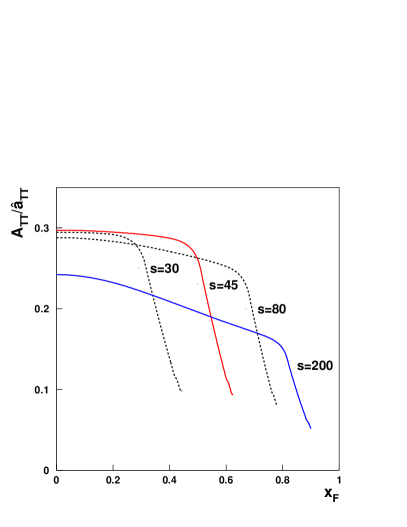
  Figure 1: Left: The kinematic region covered by the $h_{1}$ measurement at PAX in phase II. In the asymmetric collider scenario (blue) antiprotons of 15 GeV/c impinge on protons of 3.5 GeV/c at c.m. energies of $\sqrt{s}\sim\sqrt{200}$ GeV and $Q^{2}>4$ $\rm GeV^{2}$. The fixed target case (red) represents antiprotons of 22 GeV/c colliding with a fixed polarized target ($\sqrt{s}\sim\sqrt{45}$ GeV). Right: The expected asymmetry as a function of Feynman $x_{F}$ for different values of $s$ and $Q^{2}=16$ $\rm GeV^{2}$.

• The counting rates for Drell–Yan processes at PAX are estimated in Sec. 4. We notice here that in the quest for $h_{1}^{q}$ one should not confine to the $M\!>\!4$ GeV region, which is usually considered as the “safe” region for the comparison with the pQCD computations, as this cut–off eliminates the background from the $J/\Psi,\Psi^{\prime}$ production and their subsequent leptonic decay. Also the region $1.5\mathrel{\hbox to0.0pt{\lower 4.0pt\hbox{\hskip 1.0pt$\sim$}\hss}\raise 1.0pt\hbox{$<$}}M\mathrel{\hbox to0.0pt{\lower 4.0pt\hbox{\hskip 1.0pt$\sim$}\hss}\raise 1.0pt\hbox{$<$}}3$ GeV is free from resonances and can be exploited to access $h_{1}$ via Drell–Yan processes [3, 31].

• Even the $J/\Psi,\Psi^{\prime}$ resonance region at $M\simeq 3$ GeV could be crucial [2]. The cross section for dilepton production increases by almost 2 orders of magnitude going from $M=4$ to $M=3$ GeV [32, 33, 34]: this cross section involves unknown quantities related to the $q\bar{q}-J/\Psi$ coupling. However, independently of these unknown quantities, the $q\bar{q}-J/\Psi$ coupling is a vector one, with the same spinor and Lorentz structure as the $q\bar{q}-\gamma^{*}$ coupling; similarly for the $J/\Psi-e^{+}e^{-}$ decay. These unknown quantities cancel in the ratio giving $A_{TT}$, while the helicity structure remains, so that Eq. (3) still holds in the $J/\Psi$ resonance region [2]. This substantially enhances the sensitivity of the PAX experiment to $A_{TT}$ and the amount of direct information achievable on $h_{1}^{u}(x_{1},M^{2})\,h_{1}^{u}(x_{2},M^{2})$. The theoretical analysis of the NLO corrections to $A_{TT}$ for prompt photon production in hadronic collisions has already been accomplished [35], the full computation of QCD corrections to $A_{TT}$, relevant to PAX kinematical values (including the $J/\Psi,\Psi^{\prime}$ resonance region), is in progress [36].

2.3 Transversity in $D$–Meson Production at PAX

The double transverse spin asymmetry $A_{TT}$ can be studied also for other processes; in particular, the open charm production, $\bar{p}^{\uparrow}\,p^{\uparrow}\to D\,X$ looks like a very promising channel to extract further information on the transversity distributions. At PAX in collider mode ($\sqrt{s}\simeq\sqrt{210}$ GeV) the production of $D$ mesons with $p_{T}$ of the order of 2 GeV/$c$ is largely dominated by the $\bar{q}q\to\bar{c}c$ elementary process [37]; then one has (again, all distribution functions refer to protons):

$$A_{TT}^{{}^{D}}\simeq\frac{\sum_{q}h_{1}^{q}(x_{1})\otimes h_{1}^{q}(x_{2})\otimes\Delta\hat{\sigma}\otimes D(z)}{\sum_{q}q(x_{1})\otimes q(x_{2})\otimes\hat{\sigma}\otimes D}\>,$$ (4)

which supplies information about the convolution of the transversity distributions with the fragmentation functions $D(z)$ of $c$ quarks or antiquarks into $D$ mesons, which are available in the literature; $\Delta\hat{\sigma}=\hat{\sigma}^{\uparrow\uparrow}-\hat{\sigma}^{\uparrow\downarrow}$ is the known double spin asymmetry for the $\bar{q}q\to\bar{c}c$ elementary process. Eq. (4) holds above the resonance region ($M=\sqrt{x_{1}x_{2}s}\,>4$ GeV); the elementary interaction is a pQCD process, so that the cross section for $D$–production might even be larger, at the same scale, than the corresponding one for Drell–Yan processes. Notice that, once more, the same channel at RHIC cannot supply information on $h_{1}$, as at RHIC energy ($\sqrt{s}=200$ GeV), the dominant contribution to $D$ production comes from the $gg\to\bar{c}c$ elementary channel, rather than the $\bar{q}q\to\bar{c}c$ one [38].

3 Single Spin Asymmetries and Sivers Function

While the direct access to transversity is the outstanding, unique possibility offered by the PAX proposal concerning the proton spin structure, there are several other spin observables related to partonic correlation functions which should not be forgotten. These might be measurable even before the antiproton polarization is achieved.

The perturbative QCD spin dynamics, with the helicity conserving quark–gluon couplings, is very simple. However, such a simplicity does not always show up in the hadronic spin observables. The observed single spin asymmetries (SSA) are a symptom of this feature. By now it is obvious that the non–perturbative, long–distance QCD physics has many spin properties yet to be explored. A QCD phenomenology of SSA seems to be possible, but more data and new measurements are crucially needed. A new experiment with antiprotons scattered off a polarized proton target, in a new kinematical region, would certainly add valuable information on such spin properties of QCD.

As a first example we consider the transverse SSA

$$A_{N}=\frac{d\sigma^{\uparrow}-d\sigma^{\downarrow}}{d\sigma^{\uparrow}+d\sigma^{\downarrow}}\>,$$ (5)

measured in $p^{\uparrow}\,p\to\pi\,X$ and $\bar{p}^{\uparrow}\,p\to\pi\,X$ processes: the SSA at large values of $x_{F}$ ($x_{F}\mathrel{\hbox to0.0pt{\lower 4.0pt\hbox{\hskip 1.0pt$\sim$}\hss}\raise 1.0pt\hbox{$>$}}0.4$) and moderate values of $p_{T}$ ($0.7<p_{T}<2.0$ GeV/$c$) have been found by several $p^{\uparrow}\,p$ experiments [24, 25, 26] to be unexpectedly large (up to about 40$\%$), and similar values and trends of $A_{N}$ have been observed in experiments with center of mass energies ranging from 6.6 up to 200 GeV.

The large effects were unexpected because, within the standard framework of collinear QCD factorization, one has to resort to subleading twist functions in order to obtain non–zero SSA [39, 40]. However, if the factorization approach is extended to not only include longitudinal but also transverse parton momenta, non–vanishing SSA emerge already at leading twist. In such an approach the above mentioned Sivers parton distribution [4] and Collins fragmentation function [5] enter. In order to disentangle both effects the study of SSA for $D$–meson production ($\bar{p}^{\uparrow}\,p\to D\,X$ or $\bar{p}\,p^{\uparrow}\to D\,X$) is very promising. At the PAX collider energy, for a final $D$ with $p_{T}$ of about 2 GeV/c, the dominant subprocess is $\bar{q}q\to\bar{c}c$ [37], with the subsequent fragmentation of a charmed quark into a charmed meson. In this elementary annihilation process there is no transverse spin transfer and the final $c$ and $\bar{c}$ are not polarized. Therefore, there cannot be any contribution to the SSA from the Collins mechanism. A SSA could only result from the Sivers mechanism, coupled to an unpolarized elementary reaction and fragmentation. A measurement of a SSA in $\bar{p}^{\uparrow}\,p\to D\,X$ or $\bar{p}\,p^{\uparrow}\to D\,X$ would then allow a clean access to the quark Sivers function, active in an annihilation channel. This is not the case at RHIC energies, where the leading subprocess turns out to be $gg\to\bar{c}c$, which could lead to information on the gluon Sivers function [38].

The Sivers function (denoted by $f_{1T}^{\perp}$) attracted quite some interest over the past three years. It belongs to the class of the so–called (naive) time–reversal odd (T–odd) parton distributions, which are in general at the origin of SSA. Therefore, it was believed for about one decade that the Sivers function vanishes because of T–invariance of the strong interaction [5]. However, in 2002 it was shown that $f_{1T}^{\perp}$ can actually be non–zero [41, 8]. In this context it is crucial that the Wilson line, which ensures color gauge invariance, is taken into account in the operator definition of the Sivers function. The Wilson line encodes initial state interactions in the case of the Drell–Yan process and final state interactions of the struck quark in the case of DIS. The Sivers function, describing the (asymmetric) distribution of quarks in a transversely polarized nucleon [4], contains a rich amount of information on the partonic structure of the nucleon. E.g., it is related to the orbital angular momentum of partons, and the sign of the Sivers asymmetry of a given quark flavor is directly connected with the sign of the corresponding anomalous magnetic moment [42].

Figure 2: The SSA $A_{UT}^{\sin(\phi_{h}-\phi_{S})q_{\perp}/M_{N}}$ in Drell-Yan lepton pair production, $p^{\uparrow}\bar{p}\to\mu^{+}\mu^{-}X$, as function of the rapidity $y$ for typical PAX kinematics ($s=45\,\textrm{GeV}^{2}$, $M^{2}=2.5\,\textrm{GeV}^{2}$). The different curves correspond to equally good fits to the HERMES data[7].

It is now important that the Wilson line can be process dependent. This property leads to the very interesting prediction that the Sivers function in Drell–Yan and in semi–inclusive DIS (measured for instance via the transverse SSA $l\,p^{\uparrow}\to l\,\pi\,X$) should have a reversed sign [8], i.e.,

$$f_{1T}^{\perp}\Big{|}_{DY}=-f_{1T}^{\perp}\Big{|}_{DIS}\,.$$ (6)

In the meantime, the HERMES collaboration has already obtained first results for the Sivers asymmetry in semi–inclusive DIS [7]. Therefore, measuring $f_{1T}^{\perp}$ in Drell–Yan processes (like $\bar{p}\,p^{\uparrow}\to l^{+}\,l^{-}\,X$ or $\bar{p}^{\uparrow}\,p\to l^{+}\,l^{-}\,X$) at PAX would check the clear–cut prediction in Eq. (6) based on the QCD factorization approach. An experimental check of the sign–reversal would crucially test our present day understanding of T–odd parton distributions and, consequently, of the very nature of SSA within QCD. In passing, we note that, within slightly different contexts, recently several other papers have also stressed the importance of measuring SSA in Drell–Yan processes [43, 44, 45, 46, 47].

On the basis of the recent HERMES data [7] for $f_{1T}^{\perp}$ a prediction for the corresponding Sivers asymmetry in Drell Yan for PAX (for $p^{\uparrow}\bar{p}\to\mu^{+}\mu^{-}X$) has been reported [48]. The main result of this study is shown in Fig. 2, where the (weighted) asymmetry

$$A_{UT}^{\sin(\phi-\phi_{S})\frac{q_{T}}{M_{N}}}(y,M^{2})=2\;\frac{\sum_{a}e_{a}^{2}\,x_{1}f_{1T}^{\perp(1)a/p}(x_{1},M^{2})\,x_{2}f_{1}^{\bar{a}/\bar{p}}(x_{2},M^{2})}{\sum_{a}e_{a}^{2}\,x_{1}f_{1}^{a/p}(x_{1},M^{2})\,x_{2}f_{1}^{\bar{a}/\bar{p}}(x_{2},M^{2})}$$ (7)

is plotted. The weighting is performed for technical reasons and is done with $\sin(\phi-\phi_{S})$ ($\phi$ and $\phi_{S}$ respectively denoting the azimuthal angle of the virtual photon and the target spin vector), and with the transverse momentum $\vec{q}_{T}$ of the lepton pair. The quantity $f_{1T}^{\perp(1)}$ represents the second moment of the Sivers function with respect to the transverse quark momentum. In Fig. 2 the asymmetry is displayed as function of the rapidity $y$ of the lepton pair. (Note the relation $x_{1/2}=\sqrt{M^{2}/s}\,e^{\pm y}$.) On the basis of this study asymmetries of the order $5-10\%$ can be expected [48] — an effect which should definitely be measurable at PAX. This would allow one to check the predicted sign–flip of the Sivers function in the valence region, even if the error bars would be large.

In summary, combining information on SSA from $p\,p^{\uparrow}$ and $\bar{p}^{\uparrow}\,p$ processes would greatly help in disentangling the Sivers and Collins mechanism. In this context production of charmed mesons (via $\bar{p}^{\uparrow}\,p\to D\,X$ or $\bar{p}\,p^{\uparrow}\to D\,X$) can play a crucial role because these asymmetries are not sensitive to the Collins function. We have also emphasized the importance of measuring the Sivers function in Drell–Yan. Through such an experiment, in combination with the already available information on the Sivers function coming from semi–inclusive DIS, a crucial check of our current understanding of the origin of T–odd parton distributions and of SSA within QCD can be achieved in an unprecedented way.

4 Electromagnetic Form Factors of the Proton

The form factors of hadrons as measured both in the space–like and time–like domains provide fundamental information on their structure and internal dynamics. Both the analytic structure and phases of the form factors in the time–like regime are connected by dispersion relations (DR) to the space–like regime [12, 13, 14, 49, 50]. The recent experiments raised two serious issues: firstly, the Fermilab E835 measurements of $|G_{M}(q^{2})|$ of the proton at time–like $q^{2}$ = 11.63 and 12.43 GeV² ([51] and references therein) have shown that $|G_{M}(q^{2})|$ in the time–like region is twice as large as in the space–like region (there are some uncertainties because the direct $G_{E}-G_{M}$ separation was not possible due to statistics and acceptance); secondly, the studies of the electron–to–proton polarization transfer in $\overrightarrow{e}^{-}\,p\to e^{-}\,\overrightarrow{p}$ scattering at Jefferson Laboratory [9] show that the ratio of the Sachs form factors $G_{E}(q^{2})/G_{M}(q^{2})$ is monotonically decreasing with increasing $Q^{2}=-q^{2},$ in strong contradiction with the $G_{E}/G_{M}$ scaling assumed in the traditional Rosenbluth separation method, which may in fact not be reliable in the space–like region. Notice that the core of the PAX proposal is precisely the QED electron–to–nucleon polarization transfer mechanism, employed at Jefferson Laboratory.

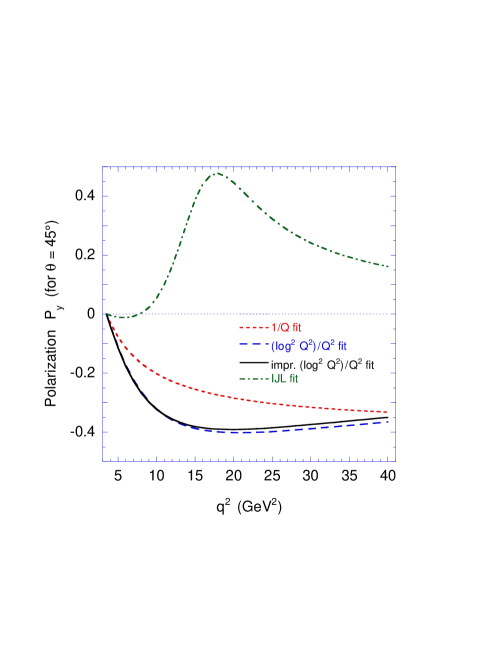
Figure 3: Predicted single–spin asymmetry ${\cal A}_{y}={\cal P}_{y}$ for $\theta=45^{\circ}$ in the time–like region for selected form factor fits: $F_{2}/F_{1}\propto 1/Q$ fit [11], the $(\log^{2}Q^{2})/Q^{2}$ fit of Belitsky et al. [52]; an improved $(\log^{2}Q^{2})/Q^{2}$ fit [53]; and a fit from Iachello et al., [54].

There is a great theoretical interest in the nucleon time–like form factors. Although the space–like form factors of a stable hadron are real, the time–like form factors have a phase structure reflecting the final–state interactions (FSI) of the outgoing hadrons. Kaidalov et al. argue that the same FSI effects are responsible for the enhancement of $|G_{M}(q^{2})|$ in the time–like region [55]; their evaluation of the enhancement based on the variation of Sudakov effects from the space–like to time–like region is consistent with general requirements from analyticity that FSI effects vanish at large $q^{2}$ in the pQCD asymptotics. A recent discussion can be found in Brodsky et al. [11] ( see also [14]). The same property of vanishing FSI at large $q^{2}$ is shared by the hybrid pQCD–DR description developed by Hammer, Meissner and Drechsel [13] and vector–dominance based models (VDM) [56], which are also able to accommodate the new results from the Jefferson Laboratory. Iachello et al. [57] stress the need for a better accuracy measurement of the neutron time–like form factors.

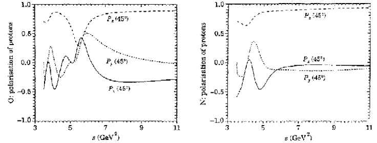
Figure 4: Predicted single–spin asymmetries (${\cal A}_{y}={\cal P}_{y}$) for $\theta=45^{\circ}$ in the time–like region for two versions (O (old) & N (new)) of the analytic and unitary vector–meson dominance (VDM) models [10]

Brodsky et al. make a strong point that the new Jefferson Laboratory results make it critical to carefully identify and separate the time–like $G_{E}$ and $G_{M}$ form factors by measuring the center–of–mass angular distribution and the polarization of the proton in $e^{+}e^{-}\to p\bar{p}$ or the transverse SSA in polarized $p^{\uparrow}\bar{p}\to\ell^{+}\ell^{-}$ reactions [11]. As noted by Dubnickova, Dubnicka, and Rekalo [10] and by Rock [58], the non–zero phase difference between $G_{E}$ and $G_{M}$ entails the normal polarization ${\cal P}_{y}$ of the final state (anti)baryons in $e^{-}e^{+}\to\overrightarrow{p}\bar{p}$ or the transverse SSA ${\cal A}_{y}={\cal P}_{y}$ in annihilation $p^{\uparrow}\bar{p}\to e^{-}e^{+}$ on transversely polarized protons:

$${\cal A}_{y}={\sin 2\theta\,{\rm Im}G_{E}^{*}G_{M}\over[(1+\cos^{2}\theta)|G_{M}|^{2}+\sin^{2}\theta|G_{E}|^{2}/\tau]\sqrt{\tau}}$$ (8)

where $\tau\equiv{q^{2}/4m_{p}^{2}}>1$ and $\theta$ is the scattering angle.

As emphasized already by Dubnickova et al. [10] the knowledge of the phase difference between the $G_{E}$ and $G_{M}$ may strongly constrain the models for the form factors. More recently there have been a number of explanations and theoretically motivated fits of the new data on the proton $F_{2}/F_{1}$ ratio [52, 59, 60, 53]. Each of the models predicts a specific fall–off and phase structure of the form factors from $s\leftrightarrow t$ crossing to the time–like domain. The predicted single–spin asymmetry is substantial and has a distinct $q^{2}$ dependence which strongly discriminates between the analytic forms which fit the proton $G_{E}/G_{M}$ data in the space–like region. This is clearly illustrated in Fig. 3. The further illustration of the discrimination power of $A_{y}$ comes from the analytic and unitary vector–meson dominance (VDM) models developed by Dubnicka et al. [10], see Fig. 4, which indicate a strong model–dependence of $P_{y}$ and more structure in the threshold region than suggested by large–$q^{2}$ parameterizations shown in Fig. 3. Finally, as argued in [61], the experimental observation of near–threshold exclusive Drell–Yan reactions $\bar{p}p\to\gamma^{*}\pi^{o}\to e^{+}e^{-}\pi^{o}$ would give unique, albeit a model-dependent, access to the proton form factors in the unphysical region of $q^{2}<4m_{p}^{2}$.

Despite the fundamental implications of the phase for the understanding of the connection between the space–like and time–like form factors, such measurements have never been made. The available data on $|G_{M}^{(p)}|$ in the time–like region are scarce, as can be seen from Fig. 5.

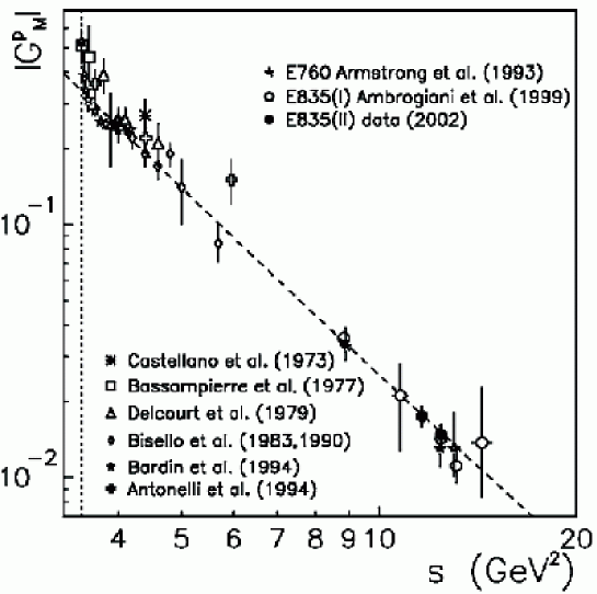
Figure 5: All existing magnetic form factor data of the proton in the time–like region obtained with the hypothesis $|G_{M}|=|G_{E}|$ versus $s=q^{2}$, as compiled in [51]; the summary of the earlier data can be found in [62].

However, these data suggest the existence of additional structures in the time–like form factor of the proton, especially in the near–threshold region; as Hammer, Meissner and Drechsel emphasized [13] that calls for improvements in the dispersion–theoretical description of form factors. We also recall recent indications for the baryonium–like states from BES in the $J/\Psi{\to}\gamma{\bar{p}}p$ decay [63] and from Belle [64, 65], which prompted much theoretical activity in low–energy proton–antiproton interactions ([66] and references therein). The phase structure of the form factors near threshold could be much richer than suggested by high–$Q^{2}$ parameterizations with an oversimplified treatment of the impact of the unphysical region.

At larger $q^{2}$ the data from E835 [62, 51] and E760 [67] seem to approach the power–law behavior predicted by pQCD. The PAX experiment would measure the relative phase $\phi_{EM}$ of the form factors from the SSA data with a transversely polarized proton target.

The modulus of $G_{E}$ and $G_{M}$ can be deduced from the angular distribution in an unpolarized measurement for $\bar{p}p\to e^{+}e^{-}$ as it can be carried out independently at PANDA as well as at PAX. However, the additional measurement of the transverse double spin asymmetry in $p^{\uparrow}\bar{p}^{\uparrow}\to\ell^{+}\ell^{-}$, that is feasible at PAX, could further reduce the systematic uncertainties of the Rosenbluth separation. We recall that, as emphasized by Tomasi–Gustaffson and Rekalo [68], the separation of magnetic and electric form factors in the time–like region allows for the most stringent test of the asymptotic regime and QCD predictions. According to Dubnicka et al. [10]

$${\cal A}_{yy}={\sin^{2}\theta\,(G_{M}|^{2}-|G_{E}|^{2}/\tau)/\rm Im\over[(1+\cos^{2}\theta)|G_{M}|^{2}+\sin^{2}\theta|G_{E}|^{2}/\tau]}\,.$$ (9)

Furthermore, in the fixed–target mode, the polarization of the proton target can readily be changed to the longitudinal direction, and the in–plane longitudinal–transverse double spin asymmetry would allow one [10] to measure ${\rm Re}G_{E}^{*}G_{M}$,

$${\cal A}_{xz}={\sin 2\theta\,{\rm Re}G_{E}^{*}G_{M}\over[(1+\cos^{2}\theta)|G_{M}|^{2}+\sin^{2}\theta|G_{E}|^{2}/\tau]},$$ (10)

which would resolve the remaining $\phi_{EM}-(\pi-\phi_{EM})$ ambiguity from the transverse SSA data. This will put tight constraints on current models of the form factor.

5 Hard Scattering: Polarized and Unpolarized

From the point of view of the theory of elastic and exclusive two–body reactions, the energy range of HESR corresponds to the transition from soft mechanisms to hard scattering with the onset of the power laws for the $s,t,u$–dependence of the differential cross sections [15, 16] which have generally been successful so far (for a review and further references see [69]). There remains, though, the open and much debated issue of the so–called Landshoff independent scattering–mechanism [18] which gives the odd–charge symmetry contribution to the $NN$ and $\bar{N}N$ amplitudes and may dominate at higher energies. The more recent realization of the importance of the so–called handbag contributions to the amplitudes of exclusive reactions made possible direct calculations of certain two–body annihilation cross sections and double–spin asymmetries in terms of the so–called Generalized Parton Distributions (GPD’s) [70, 71, 72]. The PAX experiment at HESR is uniquely poised to address several new aspects of hard exclusive scattering physics:

• The particle identification in the forward spectrometer of PAX would allow the measurement of elastic $p\bar{p}$ scattering in the small to moderately large $|t|$ in the forward hemisphere and, more interestingly, the backward hemisphere at extremely large $t$ not accessible in the $t-u$ symmetric $pp$ scattering.

• The high energy behavior of exotic baryon number, $B=2$, exchange in the $u$–channel is interesting in itself. Its measurements in the small to moderately large $u$ region of backward elastic $\bar{p}p$ scattering will be used for the isolation of hard $p\bar{p}$ scattering contribution at large $|u|$.

• After the isolation of the hard–scattering regime the importance of the odd–charge symmetry Landshoff (odderon) mechanism can be tested from the onset of the hard scattering regime in large–angle elastic $\bar{p}p$ scattering as compared to $pp$ scattering.

• The relative importance of odd–charge vs. even–charge symmetric mechanisms for the large transverse double spin asymmetry $A_{TT}$ in polarized $p^{\uparrow}p^{\uparrow}$ as observed at Argonne ZGS and BNL AGS can be clarified by a measurement of $A_{TT}$ in polarized $\bar{p}^{\uparrow}p^{\uparrow}$ elastic scattering at PAX and the comparison with the earlier data from $p^{\uparrow}p^{\uparrow}$ scattering.

• The future implementation of particle identification in the large angle spectrometer of PAX would allow an extension of measurements of elastic scattering and two–body annihilation, $\bar{p}p\to\gamma\gamma,\gamma\pi^{0},\pi^{+}\pi^{-},K^{+}K^{-},\Lambda_{c}\bar{\Lambda}_{c},...$ to large angles $\theta_{cm}\sim 90^{o}$.

• Exclusive Drell–Yan reactions with a lepton pair in the final state, accompanied by a photon or meson, may also be studied in the framework of the partonic description of baryons. Like in the conventional inclusive DY process, the large mass of the lepton pair sets the resolution scale of the inner structure of the baryon to photon or meson transition processes.

The theoretical background behind the high–$t$ or high–$Q^{2}$ ($Q^{2}=M_{e^{+}e^{-}}^{2}$) possibilities of PAX can be summarized as follows:

The scaling power law $s^{-N}$, where $N+2$ is the total number of elementary constituents in the initial and final state, for exclusive two–body hard scattering has been in the focus of high–energy scattering theory ever since the first suggestion in the early 70’s of the constituent counting rules by Matveev et al. [15] and Brodsky & Farrar [16] and Brodsky & Hiller [73]. The subsequent hard pQCD approach to the derivation of the constituent counting rules has been developed in late 70’s–early 80’s and has become known as the Efremov–Radyushkin–Brodsky–Lepage (ERBL) evolution technique ([74, 75], see also Chernyak et al. [76]). Experimentally, the constituent counting rule proves to be fairly successful, from the scattering of hadrons on protons to photoproduction of mesons [77] to reactions involving light nuclei, like the photodisintegration of deuterons studied at Jefferson Lab [78, 79] A good summary of the experimental situation is found in Ref. [80] and reviews by Brodsky and Lepage ([69] and references therein), and is summarized in Table 1, borrowed from the BNL E838 publication [80].

		Cross section		$n-2$
Experiment No. $N$	Interaction	E838	E755	$(\frac{d\sigma}{dt}\sim 1/s^{n-2})$
1	$\pi^{+}p\to p\pi^{+}$	$132\pm 10$	$4.6\pm 0.3$	$6.7\pm 0.2$
2	$\pi^{-}p\to p\pi^{-}$	$73\pm 5$	$1.7\pm 0.2$	$7.5\pm 0.3$
3	$K^{+}p\to pK^{+}$	$219\pm 30$	$3.4\pm 1.4$	$8.3^{+0.6}_{-1.0}$
4	$K^{-}p\to pK^{-}$	$18\pm 6$	$0.9\pm 0.9$	$\geq 3.9$
5	$\pi^{+}p\to p\rho^{+}$	$214\pm 30$	$3.4\pm 0.7$	$8.3\pm 0.5$
6	$\pi^{-}p\to p\rho^{-}$	$99\pm 13$	$1.3\pm 0.6$	$8.7\pm 1.0$
7	$\pi^{+}p\to\pi^{+}\Delta^{+}$	$45\pm 10$	$2.0\pm 0.6$	$6.2\pm 0.8$
8	$\pi^{-}p\to\pi^{+}\Delta^{-}$	$24\pm 5$	$\leq 0.12$	$\geq 10.1$
9	$pp\to pp$	$3300\pm 40$	$48\pm 5$	$9.1\pm 0.2$
10	$\overline{p}p\to p\overline{p}$	$75\pm 8$	$\leq 2.1$	$\geq 7.5$

Table 1: The computation of the experiments $N$ of the scaling power in the AFS BNL experiments E838 ($E_{p}=5.9$ GeV/c) and E755 ($E_{p}=9.9$ GeV/c). The constituent counting predicts $N=8$ for reactions 1 - 8 and $N=10$ for reactions 9 and 10. (Table from Ref. [80]).

The scale for the onset of the genuine pQCD asymptotics can only be deduced from the experiment, on the theoretical side the new finding is the importance of the so–called handbag mechanism in the sub–asymptotic energy range [81, 82]. As argued by P. Kroll et al., the handbag mechanism prediction for the sub–asymptotic $s$–dependence of the large–angle elastic $pp$ and $p\bar{p}$ cross–section [17] ,

$${d\sigma\over dt}\propto{1\over s^{2}t^{8}}\propto{f(\theta)\over s^{10}}$$ (11)

is similar to that of the constituent quark counting rules of Brodsky et al. [16].

There remains, though, an open and hot issue of the so–called Landshoff independent scattering–mechanism [18], which predicts ${d\sigma/dt}\propto{1/t^{8}}\propto f_{L}(\theta)/s^{8}$ and, despite the Sudakov suppression, may dominate at very large $s$. According to Ralston and Pire [19] certain evidence for the relevance of the Landshoff mechanism in the HESR energy range comes from the experimentally observed oscillatory $s$–dependence of $R_{1}=s^{10}{d\sigma/dt}$, shown in Fig. 6. Here the solid curve is the theoretical expectation [19] based on the interference of the Brodsky–Farrar and Landshoff mechanisms.

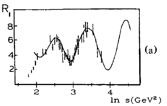
Figure 6: The energy dependence of $R_{1}=s^{10}{d\sigma_{pp}/dt}|_{90^{o}}$ for the high energy $pp$ elastic scattering at $90^{o}$ c.m. angle compared to the model calculation [19] from the interference of the Brodsky–Farrar and Landshoff mechanisms.

The Ralston–Pire mechanism has been corroborated to a certain extent by the experimental finding at BNL of the wash–up of oscillations in the quasielastic scattering of protons on protons bound in nuclei ([83] and references therein).

To the lowest order in pQCD the Landshoff amplitude corresponds to the charge conjugation–odd (odderon) exchange and alters the sign from the $pp$ to the $p\bar{p}$ case. If the Brodsky–Farrar and/or it’s handbag counterpart were crossing–even, then the Ralston–Pire scenario for the oscillations would predict the inversion of the sign of oscillation in $R_{1}$ from the $pp$ to the $p\bar{p}$ case. Because the first oscillation in Fig. 6 takes place at $s<20$ GeV², this suggests that $\bar{p}p$ elastic scattering at HESR is ideally suited for testing the oscillation scenarios. Although true in general, this expectation needs a qualification on the crossing from the proton–proton to the antiproton–proton channel. A natural origin for the constituent counting rules is offered by the quark interchange mechanism (QIM) which predicts $d\sigma_{el}(pp)\gg d\sigma_{el}(\bar{p}p)$ in accord with the experimental data from BNL E838 shown in Fig. 7.

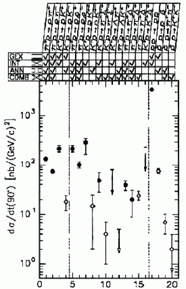
Figure 7: Differential cross sections for the 16 meson–baryon and 4 baryon–baryon reactions measured in the BNL AFS experiment E838 [80]. The four possible quark–gluon diagrams which contribute to each of the 20 reactions are given in the chart at the top of the figure. The experimental data for those reactions which have a contribution from quark interchange mechanism (INT) are shown by the solid black points.

Either the contribution from the independent scattering mechanism is small or at $E_{p}=5.9$ GeV in E838 the cancellation of the QIM and the Landshoff amplitudes is accidentally strong in which case the energy dependence of $d\sigma_{el}(\bar{p}p)$ could prove exceptionally non–smooth. On the theoretical side, as early as in 1974, Nielsen and Neal suggested the version of an independent scattering mechanism which allows for a substantial crossing–even component [84]. The Kopeliovich–Zakharov pQCD decameron (four–gluon) exchange realization [85] of the Rossi–Veneziano [86] baryon–junction, much discussed recently in view of the enhanced yield of baryons in nuclear collisions at RHIC [87], also is a multiple–scattering mechanism. The decameron amplitude decreases at large $|t|$ as slowly as the Landshoff amplitude and contributes only to the $p\bar{p}$ scattering.

The point that polarization observables are sensitive to mechanisms for the scaling behavior is conspicuous. As an example we cite the very recent experimental finding of the onset of pQCD constituent counting scaling [73] in photodisintegration of the deuteron starting from the proton transverse momentum $p_{T}$ above about 1.1 GeV [78]. On the other hand, the experimentally observed non-vanishing polarization transfer from photons to protons indicates that the observed scaling behavior is not a result of perturbative QCD [88].

Now we recall that very large double transverse asymmetries have been observed in hard proton–proton scattering ([89] and references therein). The HESR data with polarized antiprotons at PAX will complement the AGS–ZGS data in a comparable energy range. In 1974 Nielsen et al. argued [84] that within the independent scattering models the change from the dominance by $1\times 1$ parton–parton scattering to the $2\times 2$ and $3\times 3$ scattering leads in a natural way to the oscillatory ( and rising with $t$) behavior of polarization effects. Within this approach Nielsen et al. [90] reproduce the gross features of the ZGS data [89] although they underpredict $A_{TT}$ at largest $t$. Within the QCD motivated approach, initiated in Ref. [91], the helicity properties of different hard scattering mechanisms have been studied by Ramsey and Sivers [20]. These authors tried to extract the normalization of the Landshoff amplitude from the combined analysis of $pp$ and $p\bar{p}$ elastic scattering and argued it must be small to induce the oscillations or contribute substantially to the double spin asymmetry $A_{TT}$. This leaves open the origin of oscillations in $R_{1}$ but leads to the conclusion that the double spin asymmetry $A_{TT}$ in $p^{\uparrow}\bar{p}^{\uparrow}$ at PAX and $p^{\uparrow}p^{\uparrow}$ as observed at AGS–ZGS must be of comparable magnitude. The comparison of $A_{TT}$ in the two reactions will also help to constrain the Landshoff amplitude. More recently, Dutta and Gao [21] revisited the Ralston–Pire scenario with allowance for the helicity–non–conserving $pp$ scattering amplitudes (for the early discussion of helicity–non–conservation associated with the Landshoff mechanism, see Ref. [92]). They found good fits to the oscillatory behavior of $R_{1}$ and the energy dependence of $A_{TT}$ in $pp$ scattering at 90^o starting from $s\mathrel{\hbox to0.0pt{\lower 4.0pt\hbox{\hskip 1.0pt$\sim$}\hss}\raise 1.0pt\hbox{$>$}}8$ GeV². The extension of predictions from the models by Nielsen et al. and Dutta et al. to the crossing antiproton-proton channel is not yet unique, though. Brodsky and Teramond make a point that opening of the $|uuduudc\bar{c}\rangle$ channel at the open charm threshold would give rise to a broad structure in the $J=L=S=1$ proton-proton partial wave [93]. Such a threshold structure would have a negative parity and affect $p^{\uparrow}p^{\uparrow}$ scattering for parallel spins normal to the scattering plane. The threshold structure also imitates the ”oscillatory” energy dependence at fixed angle and the model is able to reproduce the gross features of the $s$ and $t$ dependence of $A_{NN}$. Arguably, in the $\bar{p}p$ channel the charm threshold is at much lower energy and the charm cross section will be much larger, and the Brodsky-Teramond mechanism would predict $A_{NN}$ quite distinct from that in $pp$ channel. Still, around the second charm threshold, $\bar{p}p\to\bar{p}p\bar{c}c$, the $A_{NN}$ for $\bar{p}p$ may repeat the behavior exhibited in $pp$ scattering.

Finally, the double–spin transverse-longitudinal asymmetry $A_{TL}$ is readily accessible in the fixed-target mode with the longitudinal polarization of the target. Its potential must not be overlooked and needs further theoretical scrutiny.

The differential cross section measured in the BNL E838 experiment is shown in Fig. 7. The expected $d\sigma/dt\propto s^{-10}$ behavior suggests that in the fixed-target Cooler Synchrotron Ring (CSR) stage (Phase-I) the counting rates will allow measurements of elastic $p\bar{p}$ scattering, both polarized and unpolarized, over the whole range of angles. In the fixed-target HESR stage the measurement of unpolarized scattering can be extended to energies beyond those of the E838 experiment. The expected counting rates will also allow the first measurement of the double–spin observables.

In the comparison of observables for the $pp$ and $\bar{p}p$ elastic scattering one would encounter manageable complications with the Pauli principle constraints in the identical particle $pp$ scattering, by which the spin amplitudes for $pp$ scattering have the $t$–$u$–(anti)symmetric form $M(\theta)\pm M(\pi-\theta)=M(t)\pm M(u)$ ([94] and references therein). Regarding the amplitude structure, the $\bar{p}p$ case is somewhat simpler and offers even more possibilities for the investigation of hard scattering. Indeed, for the hard scattering to be at work, in the general case one demands that both $|t|$ and $|u|$ are simultaneously large, $|t|\sim|u|\sim{1\over 2}(s-4m_{p}^{2})$. Here we notice an important distinction between the $t$–$u$ asymmetric $\bar{p}p$ from the $t$–$u$ symmetric identical particle $pp$ elastic scattering. In the $t$–$u$ symmetric case the accessible values of $t$ are bound from above by $|t|\leq|t_{max}|={1\over 2}(s-4m_{p}^{2})$. In the $p\bar{p}$ case the backward scattering corresponds to the strongly suppressed exotic baryon number two, $B=2$, exchange in the $u$–channel (for a discussion of the suppression of exotic exchanges see Refs. [95, 96] and references therein). Consequently, the hard scattering mechanism may dominate well beyond $\theta_{\rm cm}=90^{o}$ of $p\bar{p}$ elastic scattering. Because of the unambiguous $p$ and $\bar{p}$ separation in the forward spectrometer, the PAX will for the first time explore the transition from soft exotic $B=2$ exchange at $u\sim 0$ to the hard scattering at larger $|u|$: for 15 GeV stored $\bar{p}$’s the $p-\bar{p}$ separation is possible up to $|u|\leq 4$ GeV², while $|u|\leq 8$ GeV² is accessible at 22 GeV. Although still $|u|\ll s$, these values of $|u|$ are sufficiently large to suppress the $u$–channel exotic $B=2$ exchange, which allow the dominance of hard mechanisms, which thus become accessible at values of $|t|=s-4m_{p}^{2}-|u|$ almost twice as large than in $pp$ scattering at the same value of $s$. The investigation of the energy dependence of exotic $B=2$ exchange in the small–$u$ region is interesting by itself in order to better understand the related reactions, like the $\pi D$ backward elastic scattering.

Although not all annihilation reactions are readily accessible with the present detector configuration, they are extremely interesting from the theoretical standpoint. Within the modern handbag diagram description, they probe such fundamental QCD observables as the Generalized Parton Distributions (GPD’s), introduced by Ji and Radyushkin [70, 71]. These GPD’s generalize the conventional parton-model description of DIS to a broad class of exclusive and few–body reactions and describe off–forward parton distributions for polarized as well as unpolarized quarks; the Ferrara Manifesto, formulated at the recent Conference on the QCD Structure of the Nucleon (QCD–N’02), lists the determination of GPD’s as the major physics goal of future experiments in the electroweak physics sector [72]. The QCD evolution of GPD’s is a combination of the conventional QCD evolution for DIS parton densities and the ERBL evolution for the quark distribution amplitudes, GPD’s share with the DIS parton densities and the ERBL hard–scattering amplitudes the hard factorization theorems: the one and the same set of GPD’s at an appropriate hard scale enters the calculation of amplitudes for a broad variety of exclusive reactions.

There has been much progress in calculating the electromagnetic form factors of the nucleon and of the hard Compton scattering amplitudes in terms of the off–forward extension of the conventional parton densities [81, 82, 97, 98], Deeply Virtual Compton Scattering is being studied at all electron accelerators [99, 100] with the purpose to extract the specific GPD which would allow one to determine the fraction of the proton’s spin carried by the orbital angular momentum of partons (the Ji sum rule [70]).

More recently, the technique of GPD’s has been extended by P. Kroll and collaborators [101] to the differential cross sections and spin dependence of annihilation reactions. Here the hard scale needed for the applicability of the GPD technique is provided by $|t|$. The theory has been remarkably successful in the simplest case of $B\bar{B}\to\gamma\gamma$ with two point–like photons (the inverse reactions $\gamma\gamma\to p\bar{p}$, $\Lambda\bar{\Lambda}$, and $\Sigma\bar{\Sigma}$ have been studied experimentally by the CLEO [102] and VENUS [103] collaborations). A steady progress is being made by the DESY–Regensburg–Wuppertal group in extending these techniques to the $p\bar{p}\to\gamma\pi^{0}$ with a non–point–like $\pi^{0}$ in the final state [104], a further generalization to the two–meson final states is expected in the near future. As far as the theory of spin dependence of hard scattering is concerned the theoretical predictions are robust for the longitudinal double spin asymmetries, and thus their experimental confirmation will be of great theoretical interest. To make such observables accessible experimentally the spin of antiprotons in the HESR must be rotated by Siberian Snakes. In addition, the technique of GPD’s should allow one to relate the transverse asymmetries to the Generalized structure function $h_{1}^{q}$ (see above) but such a relationship has yet to be worked out.

A slightly different application of QCD factorization technique has been suggested recently by Pire and Szymanowski [105]. They propose to study the exclusive Drell-Yan annihilation reaction $p\bar{p}\to\gamma^{*}\gamma\to e^{+}e^{-}\gamma$. Like in the inclusive DY process, the required hard scale is provided by the large invariant mass of the lepton pair. Then one can study such reactions in the forward region which increases the observed cross section. The scaling of the cross section at fixed $Q^{2}/s$ is then a signal of the applicability of perturbative QCD techniques. New observables, called proton to photon transition distribution amplitudes (TDA’s), may then be measured which should shed light on the structure of the baryon wave functions. Polarization experiments are needed to separate the different TDA’s. The same theoretical framework can also be applied to other reactions involving mesons in the final state, like $p\bar{p}\to\gamma^{*}\pi$ or $p\bar{p}\to\gamma^{*}\rho$ [106] (the former reaction has already been discussed in Sect. 4 as a window to the time-like form factors of the proton in the unphysical region). Crossing relates these reactions to backward deep electroproduction which may be accessed at electron accelerators.

6 Polarized Antiproton–Proton Soft Scattering

6.1 Low–$t$ Physics

For energies above the resonance region elastic scattering is dominated by small momentum transfers and therefore total elastic cross sections are basically sensitive to the small $t$ region only.

Dispersion theory (DT) is based on a generally accepted hypothesis that scattering amplitudes are analytic in the whole Mandelstam plane up to singularities derived from unitarity and particle/bound state poles. This, in combination with unitarity and crossing symmetry, allows extracting of e.g. the real part of the forward elastic scattering amplitude from knowledge of the corresponding total cross sections. The major unknown in this context is the unphysical region: a left hand cut that starts at the two pion production threshold and extends up to the $\bar{N}N$ threshold, where one is bound to theoretical models for the discontinuity; the extrapolation to asymptotic energies is considered to be well understood [107] and does not effect the DT predictions in the HESR energy range.

Under certain assumptions, the real part of the forward scattering amplitude can be extracted from the elastic differential cross section measured in the Coulomb-nuclear interference (CNI) region ([108] and references therein). The most recent DT analysis [22] reproduces the gross features of the available data, see Fig. 8; still, the experiment suggests more structure at low energies (which may be related to the near-threshold structure in the electromagnetic form factor shown in Fig. 5) and there is a systematic departure of the theoretical prediction from the experiment in the region between 1 and 10 GeV/c. In particular the latest precise results from Fermilab E760 Collaboration [23] collected in the 3.7 to 6.2 GeV/c region are in strong disagreement with DT.

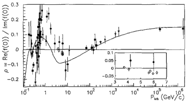
Figure 8: The compilation of the experimental data on the ratio of the real to imaginary part of the $\bar{p}p$ forward scattering amplitude (from E760 publication [23]). The insert shows on a larger scale the E760 results. The solid line shows the predictions from the dispersion relation calculation by P. Kroll et al. [22].

There are two explanations possible for this discrepancy. First one might doubt the theoretical understanding of the amplitude in the unphysical region. In this sense the DT analysis is a strong tool to explore the unphysical region. Since the discrepancy of the data to the result of the DT analysis occurs in a quite confined region, only a very pronounced structure in the unphysical region could be the origin. Such a structure can be an additional pole related to a $\bar{p}p$ bound state, discussed in Refs. [109, 110, 111, 112]. The appearance of a pole in the unphysical region might cause a turnover of the real part of the forward scattering amplitude to small values at momenta above 600 MeV/c [113, 114]. Indications of such states were seen recently at BES in the $J/\Psi{\to}\gamma{\bar{p}}p$ decay [63] and Belle [64, 65] and attracted much theoretical attention ([66] and references therein).

However, there is a second possible reason for the discrepancy of the DT result and the data, namely that not all assumptions in the analysis of CNI hold, the strongest one being a negligible spin dependence in the nuclear interference region [115]. A sizable spin dependence of the nuclear amplitude can well change the analysis used in Ref. [23]; such a sensitivity to a possible spin dependence has been discussed earlier [116]. The quantities to be measured are $\Delta\sigma_{T}=\sigma(\uparrow\downarrow)-\sigma(\uparrow\uparrow)$ and $\Delta\sigma_{L}=\sigma(\rightleftarrows)-\sigma(\rightrightarrows)$: their knowledge will eliminate the model–dependent extraction of the real part of the $p\bar{p}$ scattering amplitude [117]. Please note that a sizable value of $\Delta\sigma_{T}$ or $\Delta\sigma_{L}$ at high energies is an interesting phenomenon in itself since it contradicts the generally believed picture that spin effects die out with increasing energy (see also previous section).

Thus, a measurement of $\Delta\sigma_{L/T}$ in the energy region accessible at HESR not only allows one to investigate spin effects of the $\bar{p}p$ interaction at reasonably high energies but also to pin down the scattering amplitude in the unphysical region to deepen our understanding of possible $\bar{p}p$ bound states. Especially a determination of $\Delta\sigma_{T}$ can be done in a straightforward way as outlined in the next section. The low-$t$ physics program is ideally suited for the Phase–I with the polarized fixed target at CSR, and can further be extended to Phase–II.

6.2 Total Cross Section Measurement

The unpolarized total cross section $\sigma_{\rm 0,tot}$ has been measured at several laboratories over the complete HESR momentum range; however, the spin dependent total cross section is comprised of three parts [118]

$$\sigma_{\rm tot}=\sigma_{\rm 0,tot}+\sigma_{\rm 1,tot}\vec{P}\cdot\vec{Q}+\sigma_{\rm 2,tot}(\vec{P}\cdot\hat{k})(\vec{Q}\cdot\hat{k}).$$ (12)

where $\vec{P},\vec{Q}$ are the beam and target polarizations and $\hat{k}$ the unit vector along the beam momentum. Note that the spin–dependent contributions $\sigma_{1,2}$ are completely unexplored over the full HESR energy range. Only one measurement at much higher energies from E704 at 200 GeV/c [119] has been reported using polarized antiprotons from parity–non–conserving $\bar{\Lambda}$–decays.

With the PAX detector the transverse cross section difference $\Delta\sigma_{T}=-2\sigma_{\rm 1,tot}$ can be accessed by two methods:

• from the rate of polarization buildup for a transversely polarized target when only a single hyperfine state is used. The contribution from the electrons is known from theory and can be subtracted. However, the difference of the time constants for polarization buildup with hyperfine states 1 or 2 (cf. Fig. 11) injected into the target, would give direct access to $\Delta\sigma_{T}$, whereas the contribution from the electrons could be extracted from the average.

• from the difference in beam lifetime for a target polarization parallel or antiparallel to the beam. A sensitive beam–current transformer (BCT) can measure beam lifetimes of the antiproton beam after polarization and ramping to the desired energy. An accuracy at the $10^{-4}$ level has been achieved by the TRIC experiment at COSY using this method. Access to $\Delta\sigma_{T}$ by this technique is limited to beam momenta where losses are dominated by the nuclear cross section, e.g. above a few GeV/c – the precise limit will be determined by the acceptance of the HESR.

Both methods require knowledge of the total polarized target thickness exposed to the beam. With a calibrated hydrogen source fed into the storage cell, the target density can be determined to 2–3% as shown by the HERMES [120] and FILTEX [121] experiments.

In principle, $\Delta\sigma_{L}=-2(\sigma_{\rm 1,tot}+\sigma_{\rm 2,tot})$ can be measured by the same method; however, a Siberian snake would be needed in the ring to allow for a stable longitudinal polarization at the interaction point.

6.3 Proton–Antiproton Interaction

The main body of $\bar{N}N$ scattering data has been measured at LEAR (see [122] for a recent review) and comprises mainly cross section and analyzing power data, as well as a few data points on depolarization and polarization transfer. These data have been interpreted by phenomenological or meson–exchange potentials by exploiting the G–parity rule, linking the $\bar{N}N$ and the $NN$ systems.

At the HESR the spin correlation parameters $A_{\rm NN}$, $A_{\rm SS}$, and $A_{\rm SL}$ can be accessed for the first time by PAX which would add genuine new information on the spin dependence of the interaction and help to pin down parameters of phenomenological $\bar{N}N$ models. This part of the program will start with the polarized fixed-target experiments with polarized antiprotons in CSR (Phase–I) and can be extended to Phase–II.

Besides, available data on the analyzing power from LEAR will be used for polarimetry to obtain information on the target and beam polarization, independent from the polarimeter foreseen for the polarized target (cf. Sec. 11).

Part II Polarized Antiprotons at FAIR

7 Overview

A viable practical scheme which allows us to reach a polarization of the stored antiprotons at HESR–FAIR of $\simeq 0.3$ has been worked out and published in Ref. [123]. The basic approach to polarizing and storing antiprotons at HESR–FAIR is based on solid QED calculations of the spin transfer from electrons to antiprotons [124, 125], which is being routinely used at Jefferson Laboratory for the electromagnetic form factor separation [126], and which has been tested and confirmed experimentally in the FILTEX experiment [121].

The PAX Letter–of–Intent was submitted on January 15, 2004. The physics program of PAX has been reviewed by the QCD Program Advisory Committee (PAC) on May 14–16, 2004 [127]. The proposal by the ASSIA collaboration [128] to utilize a polarized solid target and to bombard it with a 45 GeV unpolarized antiproton beam extracted from the synchrotron SIS100 has been rejected by the GSI management. Such measurements would not allow one to determine $h^{q}_{1}(x,Q^{2})$, because in single spin measurements $h^{q}_{1}(x,Q^{2})$ appears always coupled to another unknown fragmentation function. Following the QCD–PAC report and the recommendation of the Chairman of the committee on Scientific and Technological Issues (STI) and the FAIR project coordinator [127], the PAX collaboration has optimized the technique to achieve a sizable antiproton polarization and is presenting here an updated proposal for experiments at GSI with polarized antiprotons [123]. From various working group meetings of the PAX collaboration, presented in part in 2004 at several workshops and conferences [127], we conclude:

• Polarization buildup in the HESR ring, operated at the lowest possible energy, as discussed in PAX LoI, does not allow one to achieve the optimum degree of polarization in the antiproton beam. The goal of achieving the highest possible polarization of antiprotons and optimization of the figure of merit dictates that one polarizes antiprotons in a dedicated low–energy ring (APR). The transfer of polarized low–energy antiprotons into the HESR ring requires pre–acceleration to about 1.5 GeV/c in a dedicated booster ring (CSR). Simultaneously, the incorporation of this booster ring into the HESR complex opens up, quite naturally, the possibility of building an asymmetric antiproton–proton collider.

The TSR experiment [121] and the analysis of the TSR results by Meyer and Horowitz [124, 125] have shown that several mechanisms contribute to the buildup of polarization, i.e., polarization dependent removal, small–angle scattering into–the–beam, and interaction with the polarized electrons of the target atoms. In the case of stored protons, the three mechanisms are of comparable strength, a comparison of the mechanisms for antiprotons is discussed in Sec. B.3. As a reference point, we discuss below the electromagnetic transfer of the electron polarization to scattered antiprotons.

The PAX collaboration proposes an approach that is composed of two phases. During these the major milestones of the project can be tested and optimized before the final goal is approached: An asymmetric proton–antiproton collider, in which polarized protons with momenta of about 3.5 GeV/c collide with polarized antiprotons with momenta up to 15 GeV/c. These circulate in the HESR, which has already been approved and will serve the PANDA experiment. In the following, we will briefly describe the overall machine setup of the APR, CSR, and HESR complex, schematically depicted in Fig. 9.

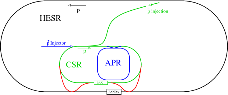
Figure 9: The proposed accelerator set–up at the HESR (black), with the equipment used by the PAX collaboration in Phase–I: CSR (green), APR, beam transfer lines and polarized proton injector (all blue). In Phase–II, by adding two transfer lines (red), an asymmetric collider is set up. It should be noted that, in this phase, also fixed target operation at PAX is possible. (The figure is drawn to scale.)

The main features of the accelerator setup are:

1. An Antiproton Polarizer Ring (APR) built inside the HESR area with the crucial goal of polarizing antiprotons at kinetic energies around $\approx 50$ MeV (see Table 3), to be accelerated and injected into the other rings.

2. A second Cooler Synchrotron Ring (CSR, COSY–like) in which protons or antiprotons can be stored with a momentum up to 3.5 GeV/c. This ring shall have a straight section, where a PAX detector could be installed, running parallel to the experimental straight section of HESR.

3. By deflection of the HESR beam into the straight section of the CSR, both the collider or the fixed–target mode become feasible.

It is worthwhile to stress that, through the employment of the CSR, effectively a second interaction point is formed with minimum interference with PANDA. The proposed solution opens the possibility to run two different experiments at the same time. In order to avoid unnecessary spin precession, all rings, ARP, CSR and HESR, should be at the same level such that no vertical deflection is required when injecting from one ring into the other.

In Sec. III, we discuss the staging of the physics program, which should be pursued in two phases.

8 Antiproton Polarizer Ring

For more than two decades, physicists have tried to produce beams of polarized antiprotons [129]. Conventional methods like atomic beam sources (ABS), appropriate for the production of polarized protons and heavy ions cannot be applied, since antiprotons annihilate with matter. Polarized antiprotons have been produced from the decay in flight of $\bar{\Lambda}$ hyperons at Fermilab. The achieved intensities with antiproton polarizations $P>0.35$ never exceeded $1.5\cdot 10^{5}$ s^-1 [130]. Scattering of antiprotons off a liquid hydrogen target could yield polarizations of $P\approx 0.2$, with beam intensities of up to $2\cdot 10^{3}$ s^-1 [131]. Unfortunately, both approaches do not allow efficient accumulation in a storage ring, which would greatly enhance the luminosity. Spin splitting using the Stern–Gerlach separation of the given magnetic substates in a stored antiproton beam was proposed in 1985 [132]. Although the theoretical understanding has much improved since then [133], spin splitting using a stored beam has yet to be observed experimentally.

8.1 The Polarizing Process $\bar{p}+\vec{e}\to\vec{\bar{p}}+e$

In 1992 an experiment at the Test Storage Ring (TSR) at MPI Heidelberg showed that an initially unpolarized stored 23 MeV proton beam can be polarized by spin–dependent interaction with a polarized hydrogen gas target [121, 134, 135]. In the presence of polarized protons of magnetic quantum number ${m=\frac{1}{2}}$ in the target, beam protons with ${m=\frac{1}{2}}$ are scattered less often, than those with ${m=-\frac{1}{2}}$, which eventually caused the stored beam to acquire a polarization parallel to the proton spin of the hydrogen atoms during spin filtering.

In an analysis by Meyer three different mechanisms were identified, that add up to the measured result [124]. One of these mechanisms is spin transfer from the polarized electrons of the hydrogen gas target to the circulating protons. Horowitz and Meyer derived the spin transfer cross section ${p+\vec{e}\rightarrow\vec{p}+e}$ (using ${c=\hbar=1}$) [125],

$$\sigma_{e_{||}}=-\frac{4\pi\alpha^{2}(1+a)m_{e}}{p^{2}m_{p}}\cdot C_{0}^{2}\cdot\frac{v}{2\alpha}\cdot\sin\left(\frac{2\alpha}{v}\ln(2pa_{0})\right)\;,$$ (13)

where ${\alpha}$ is the fine–structure constant, $a=\frac{g-2}{2}=1.793$ is the anomalous magnetic moment of the proton, ${m_{e}}$ and ${m_{p}}$ are the rest mass of electron and proton, ${p}$ is the momentum in the CM system, ${a_{0}=52900\;{\rm fm}}$ is the Bohr radius and ${C_{0}^{2}=2\pi\eta/[\exp(2\pi\eta)-1]}$ is the square of the Coulomb wave function at the origin. The Coulomb parameter ${\eta}$ is given by ${\eta=-z\alpha/v}$ (for antiprotons, $\eta$ is positive). ${z}$ is the beam charge number and ${v}$ the relative velocity of particle and projectile. In Fig. 10 the spin transfer cross section

Figure 10: Spin transfer cross section ${\sigma_{e_{||}}}$ of antiprotons scattered from longitudinally polarized electrons ${(\bar{p}+\vec{e}\rightarrow\vec{\bar{p}}+e)}$ as a function of the kinetic energy of the antiprotons.

${\sigma_{e_{||}}}$ of antiprotons scattered from longitudinally polarized electrons is plotted versus the beam kinetic energy ${T}$.

8.2 Design Consideration for the APR

In the following we evaluate a concept for a dedicated antiproton polarizer ring (APR). Antiprotons would be polarized by the spin–dependent interaction in an electron–polarized hydrogen gas target. This spin–transfer process is calculable, whereas, due to the absence of polarized antiproton beams in the past, a measurement of the spin–dependent $\bar{p}p$ interaction is still lacking, and only theoretical models exist [136]. The polarized antiprotons would be subsequently transferred to the HESR for measurements (Fig. 9).

Both the APR and the HESR should be operated as synchrotrons with beam cooling to counteract emittance growth. In both rings the beam polarization should be preserved during acceleration without loss [137]. The longitudinal spin–transfer cross section is twice as large as the transverse one [124], $\sigma_{e_{\parallel}}=2\cdot\sigma_{e_{\bot}}$, the stable spin direction of the beam at the location of the polarizing target should therefore be longitudinal as well, which requires a Siberian snake in a straight section opposite the polarizing target [138].

8.2.1 Polarizer Target

A hydrogen gas target of suitable substate population represents a dense target of quasi–free electrons of high polarization and areal density. Such a target can be produced by injection of two hyperfine states with magnetic quantum numbers $|m_{J}=+\frac{1}{2},m_{I}=+\frac{1}{2}\rangle$ and $|+\frac{1}{2},-\frac{1}{2}\rangle$ into a strong longitudinal magnetic holding field of about $B_{||}=300$ mT (Fig. 11).

Figure 11: Breit–Rabi diagram of hydrogen atoms in units of ${\Delta W=h\times 1420.4\;\mathrm{MHz}}$ [139]. The magnetic field is given in units of ${\chi=B/B_{\mathrm{c}}}$. The critical field for the ground state of hydrogen is ${B_{c}=50.7\;{\rm mT}}$.

The maximum electron and nuclear target polarizations in such a field are $Q_{e}=0.5\cdot(1+\chi/\sqrt{1+\chi^{2}})=0.993$ and $Q_{z}=0.5\cdot(1-\chi/\sqrt{1+\chi^{2}})=0.007$ [139], where $\chi=B_{||}/B_{c}$ and $B_{c}=50.7$ mT. Polarized atomic beam sources presently produce a flux of hydrogen atoms of about $q=1.2\cdot 10^{17}$ atoms/s in two hyperfine states [140]. Our model calculation for the polarization buildup assumes a moderate improvement of 20%, i.e. a flow of $q=1.5\cdot 10^{17}$ atoms/s.

8.2.2 Beam Lifetime in the APR

The beam lifetime in the APR can be expressed as function of the Coulomb–loss cross section $\Delta\sigma_{C}$ and the total hadronic $\bar{p}p$ cross section $\sigma_{\mathrm{tot}}$,

$$\tau_{\mathrm{APR}}=\frac{1}{(\Delta\sigma_{C}+\sigma_{\mathrm{tot}})\cdot d_{t}\cdot f_{\mathrm{APR}}}\;.$$ (14)

The density $d_{t}$ of a storage cell target depends on the flow of atoms $q$ into the feeding tube of the cell, its length along the beam $L_{\mathrm{beam}}$, and the total conductance $C_{\mathrm{tot}}$ of the storage cell $d_{t}=\frac{1}{2}\frac{L_{\mathrm{beam}}\cdot q}{C_{\mathrm{tot}}}$ [141]. The conductance of a cylindrical tube $C_{\mathrm{\circ}}$ for a gas of mass $M$ in the regime of molecular flow (mean free path large compared to the dimensions of the tube) as function of its length $L$, diameter $d$, and temperature $T$, is given by $C_{\mathrm{\circ}}=3.8\cdot\sqrt{\frac{T}{M}}\cdot\frac{d^{3}}{L+\frac{4}{3}\cdot d}.$ The total conductance $C_{\mathrm{tot}}$ of the storage cell is given by $C_{\mathrm{tot}}=C_{\mathrm{\circ}}^{\mathrm{feed}}+2\cdot C_{\mathrm{\circ}}^{\mathrm{beam}},$ where $C_{\mathrm{\circ}}^{\mathrm{feed}}$ denotes the conductance of the feeding tube and $C_{\mathrm{\circ}}^{\mathrm{beam}}$ the conductance of one half of the beam tube. The diameter of the beam tube of the storage cell should match the ring acceptance angle $\Psi_{\mathrm{acc}}$ at the target, $d_{\mathrm{beam}}=2\cdot\Psi_{\mathrm{acc}}\cdot\beta$, where for the $\beta$–function at the target, we use $\beta=\frac{1}{2}\,L_{\mathrm{beam}}$. One can express the target density in terms of the ring acceptance, $d_{t}\equiv d_{t}(\Psi_{\mathrm{acc}})$, where the other parameters used in the calculation are listed in Table 2.

circumference of APR	$L_{\mathrm{APR}}$	150 m
$\beta$–function at target	$\beta$	0.2 m
radius of vacuum chamber	$r$	5 cm
gap height of magnets	$2\,g$	14 cm
ABS flow into feeding tube	$q$	$1.5\cdot 10^{17}$ atoms/s
storage cell length	$L_{\mathrm{beam}}$	40 cm
feeding tube diameter	$d_{\mathrm{feed}}$	1 cm
feeding tube length	$L_{\mathrm{feed}}$	15 cm
longitudinal holding field	$B_{||}$	300 mT
electron polarization	$Q_{e}$	0.9
cell temperature	$T$	100 K

Table 2: Parameters of the APR and the polarizing target section.

The Coulomb–loss cross section $\Delta\sigma_{C}$ (using ${c=\hbar=1}$) can be derived analytically in terms of the square of the total energy $s$ by integration of the Rutherford cross section, taking into account that only those particles are lost that undergo scattering at angles larger than $\Psi_{\mathrm{acc}}$,

$$\Delta\sigma_{C}(\Psi_{\mathrm{acc}})=4\pi\alpha^{2}\frac{(s-2m_{\bar{p}}^{2})^{2}\,4m_{\bar{p}}^{2}}{s^{2}(s-4m_{\bar{p}}^{2})^{2}}\,\left(\frac{1}{\Psi_{\mathrm{acc}}^{2}}-\frac{s}{4m_{\bar{p}}^{2}}\right)\;.$$ (15)

The total hadronic cross section is parameterized using a function inversely proportional to the Lorentz parameter $\beta_{\mathrm{lab}}$. Based on the $\bar{p}p$ data [142] the parameterization $\sigma_{\mathrm{tot}}=\frac{75.5}{\beta_{\mathrm{lab}}}\;(\mathrm{mb})$ yields a description of $\sigma_{\mathrm{tot}}$ with $\approx 15$% accuracy up to $T\approx 1000$ MeV. The APR revolution frequency is given by

$$f_{\mathrm{APR}}=\frac{\beta_{\mathrm{lab}}\cdot c}{L_{\mathrm{APR}}}\;.$$ (16)

The resulting beam lifetime in the APR as function of the kinetic energy $T$ is depicted in Fig. 12 for different acceptance angles $\Psi_{\mathrm{acc}}$.

Figure 12: Beam lifetime in the APR as function of kinetic energy $T$. From top to bottom the lines denote $\Psi_{\mathrm{acc}}=50$, 40, 30, 20, and 10 mrad.

8.3 Polarization Buildup

The buildup of polarization due to the spin–dependent $\bar{p}e$ interaction in the target [Eq. (13)] as function of time $t$ is described by

$$P(t)=\tanh\left(\frac{t}{\tau_{p}}\right)\;,\,\mathrm{where}\;\tau_{p}=\frac{1}{\sigma_{e_{\parallel}}\,d_{t}\,f_{\mathrm{APR}}\,Q_{e}}$$ (17)

denotes the polarization buildup time. The time dependence of the beam intensity is described by

$$I(t)=I_{0}\cdot\exp{\left(-\frac{t}{\tau_{\mathrm{APR}}}\right)}\cdot\cosh{\left(\frac{t}{\tau_{p}}\right)}\;,$$ (18)

where $I_{0}=N_{\bar{p}}^{\mathrm{APR}}\cdot f_{\mathrm{APR}}$. The quality of the polarized antiproton beam can be expressed in terms of the figure of merit [143]

$$\mathrm{FOM}(t)=P(t)^{2}\cdot I(t)\;.$$ (19)

The optimum interaction time $t_{\mathrm{opt}}$, where $\mathrm{FOM}(t)$ reaches the maximum, is given by $\frac{\mathrm{d}}{\mathrm{d}\,t}\mathrm{FOM}(t)=0$. For the situation discussed here, $t_{\mathrm{opt}}=2\cdot\tau_{\mathrm{APR}}$ constitutes a good approximation that deviates from the true values by at most 3%. The magnitude of the antiproton beam polarization $P(t_{\mathrm{opt}})$ based on electron spin transfer [Eq. (17)] is depicted in Fig. 13 as function of beam energy $T$ for different acceptance angles $\Psi_{\mathrm{acc}}$.

Figure 13: Antiproton beam polarization $P(2\cdot\tau_{\mathrm{APR}})$ [Eq. (17)] as function of beam energy for different acceptance angles $\Psi_{\mathrm{acc}}$. (Lines are organized as in Fig. 12.)

8.3.1 Space–Charge Limitations

The number of antiprotons stored in the APR may be limited by space–charge effects. With an antiproton production rate of $R=10^{7}$ $\bar{p}/s$, the number of antiprotons available at the beginning of the filtering procedure corresponds to

$$N_{\bar{p}}^{\mathrm{APR}}(t=0)=R\cdot 2\cdot\tau_{\mathrm{APR}}\;.$$ (20)

The individual particle limit in the APR is given by [144]

$$N_{\mathrm{ind.}}=2\,\pi\,\varepsilon\,\beta_{\mathrm{lab}}^{2}\,\gamma_{\mathrm{lab}}^{3}\,(r_{p}\,F)^{-1}\,\Delta Q\;,$$ (21)

where $\varepsilon=\Psi_{\mathrm{acc}}^{2}\cdot\beta$ denotes the vertical and horizontal beam emittance, $\beta_{\mathrm{lab}}$ and $\gamma_{\mathrm{lab}}$ are the Lorentz parameters, $r_{p}=1.5347\cdot 10^{-18}$ m is the classical proton radius, and $\Delta Q=0.01$ is the allowed incoherent tune spread. The form factor $F$ for a circular vacuum chamber [144] is given by $F=1+\left(a_{y}\cdot\frac{a_{x}+a_{y}}{r^{2}}\right)\cdot\varepsilon_{2}\cdot(\gamma_{\mathrm{lab}}^{2}-1)\cdot\frac{r^{2}}{g^{2}}$, where the mean semi–minor horizontal $(x)$ and vertical $(y)$ beam axes $a_{x,y}=\sqrt{\varepsilon\cdot\beta_{x,y}}$ are calculated from the mean horizontal and vertical $\beta$–functions $\beta_{x,y}=L_{\mathrm{APR}}\cdot(2\pi\nu)^{-1}$ for a betatron–tune $\nu=3.6$. For a circular vacuum chamber and straight magnet pole pieces the image force coefficient $\varepsilon_{2}=0.411$. The parameter $r$ denotes the radius of the vacuum chamber and $g$ half of the height of the magnet gaps (Table 2). In Fig. 14 the individual particle limit is plotted for the different acceptance angles.

Figure 14: Individual particle limit $N_{\mathrm{{ind.}}}$ for the five different ring acceptance angles $\Psi_{\mathrm{acc}}$ (50 – 10 mrad) as function of beam energy. (Lines are organized as in Fig. 12.)

8.3.2 Optimum Beam Energies for the Polarization Buildup

The optimum beam energies for different acceptance angles at which the polarization buildup works best, however, cannot be obtained from the maxima in Fig. 13. In order to find these energies, one has to evaluate at which beam energies the FOM [Eq. (19)], depicted in Fig. 15, reaches a maximum. The optimum beam energies for polarization buildup in the APR are listed in Table 3. The limitations due to space–charge, $N_{\bar{p}}^{\mathrm{APR}}>N_{\mathrm{ind.}}$ [Eqs. (20, 21)], are visible as kinks in Fig. 15 for the acceptance angles $\Psi_{\mathrm{acc}}=40$ and 50 mrad, however, the optimum energies are not affected by space–charge.

Figure 15: Figure of Merit for the polarized antiproton beam for filtering times $t=2\cdot\tau_{\mathrm{APR}}$ as function of beam energy. The parameters associated with the maxima are summarized in Table 3. (Lines are organized as in Fig. 12.)

$\Psi_{\mathrm{acc}}$ (mrad)	$T$ (MeV)	$\tau_{\mathrm{APR}}$ (h)	$P(2\,\tau_{\mathrm{APR}})$
10	167	1.2	0.19
20	88	2.2	0.29
30	61	4.6	0.35
40	47	9.2	0.39
50	39	16.7	0.42

Table 3: Kinetic beam energies where the polarized antiproton beam in the APR reaches the maximum FOM for different acceptance angles.

8.3.3 Polarized Targets containing only Electrons

Spin filtering in a pure electron target greatly reduces the beam losses, because $\sigma_{\mathrm{tot}}$ disappears and Coulomb scattering angles in $\bar{p}e$ collisions do not exceed $\Psi_{\mathrm{acc}}$ of any storage ring. With stationary electrons stored in a Penning trap, areal densities of about $10^{12}$ electrons/cm² may be reached in the future [145]. A typical electron cooler operated at 10 kV with polarized electrons of intensity $\approx 1$ mA ($I_{e}\approx 6.2\cdot 10^{15}$ electrons/s) [146], $A=1$ cm² cross section, and $l=5$ m length reaches $d_{t}=I_{e}\cdot l\cdot(\beta_{\mathrm{lab}}\,c\,A)^{-1}=5.2\cdot 10^{8}$ electrons/cm², which is six orders of magnitude short of the electron densities achievable with a neutral hydrogen gas target. For a pure electron target the spin transfer cross section is $\sigma_{e_{||}}=670$ mb (at $T=6.2$ MeV) [125], about a factor $15$ larger than the cross sections associated to the optimum energies using a gas target (Table 3). One can therefore conclude that with present day technologies, both above discussed alternatives are no match for spin filtering using a polarized gas target.

8.4 Luminosity Estimate for a Fixed Target in the HESR

In order to estimate the luminosities, we use the parameters of the HESR ($L_{\mathrm{HESR}}=440$ m). After spin filtering in the APR for $t_{\mathrm{opt}}=2\cdot\tau_{\mathrm{APR}}$, the number of polarized antiprotons transfered to HESR is $N_{\bar{p}}^{\mathrm{APR}}(t=0)/e^{2}$ [Eq. (20)]. The beam lifetime in the HESR at $T=15$ GeV for an internal polarized hydrogen gas target of $d_{t}=7\cdot 10^{14}$ cm^-2 is about $\tau_{\mathrm{HESR}}=12$ h [Eqs. (14, 16)], where the target parameters from Table 2 were used, a cell diameter $d_{\mathrm{beam}}=0.8$ cm, and $\sigma_{\mathrm{tot}}=50$ mb. Subsequent transfers from the APR to the HESR can be employed to accumulate antiprotons. Eventually, since $\tau_{\mathrm{HESR}}$ is finite, the average number of antiprotons reaches equilibrium, $\overline{N_{\bar{p}}^{\mathrm{HESR}}}=R/e^{2}\cdot\tau_{\mathrm{HESR}}=5.6\cdot 10^{10}$, independent of $\tau_{\mathrm{APR}}$. An average luminosity of $\bar{{\cal L}}=R/(e^{2}\cdot\sigma_{\mathrm{tot}})=2.7\cdot 10^{31}\;\mathrm{cm}^{-2}\mathrm{s}^{-1}\$ can be achieved, with antiproton beam polarizations depending on the APR acceptance angle $\Psi_{\mathrm{acc}}$ (Table 3).

To summarize, we have shown that with a dedicated large acceptance antiproton polarizer ring ($\Psi_{\mathrm{acc}}=10$ to 50 mrad), beam polarizations of $P=0.2$ to 0.4 could be reached. The energies at which the polarization buildup works best range from $T=40$ to 170 MeV. In equilibrium, the average luminosity for double–polarization experiments in an experimental storage ring (e.g. HESR) after subsequent transfers from the APR could reach $\bar{{\cal L}}=2.7\cdot 10^{31}\;\mathrm{cm}^{-2}\mathrm{s}^{-1}$.

8.5 Technical Realization of the APR

Antiprotons are conveniently polarized at an energy of $\approx 50$ MeV ($\beta_{c}=0.28$) with an adequate gas target [141]. A storage ring is ideal to efficiently achieve a high degree of beam polarization due to the repeated beam traversal of the target. The beam degradation, the geometrical blow–up, and the subsequent smearing of the beam energy needs to be corrected by phase–space cooling, preferably by electron cooling. The shaking of the beam [147], leading to unwanted instabilities caused by positive ions accumulated around the beam, can be eliminated by a suitable RF cavity. Since the antiprotons should be longitudinally polarized, the ring has to contain a Siberian snake [138]. Finally efficient systems for injection and extraction of the antiproton beam have to be provided in the ring as well. The consequences of these insertions are at first, sufficient space in the ring and secondly, various specifications of the antiproton beam at the positions of these insertions, i.e. constraints on the ion–optical parameters. Obviously, for a high antiproton polarization, the divergence of the beam at the polarizer target should be large. The antiproton beam will be injected by stacking in phase space. The extraction will be done by bunch–to–bunch transfer. In the empty ring, the antiproton beam lifetime should be a several tens of hours, which sets also the requirements for the vacuum system.

The antiproton polarizer, discussed here, would provide highly polarized antiproton beams of unprecedented quality. In particular the implementation of this option at the Facility for Antiproton and Ion Research would open new and unique research opportunities for spin–physics experiments in $\bar{p}p$ interactions at the HESR and CSR.

8.5.1 Constraints

Following the known requests, we describe here a design for such a ring. Four straight sections are required for the following insertions:

1. Injection and extraction of the antiproton beam, for which free space of 4 m is foreseen.

2. For the gas target a low $\beta$–section is required in order to obtain a small beam spot and a large angular divergence, in this straight section a free space of 1 m is provided.

3. The opposite straight section should be reserved for the Siberian snake to longitudinally align the antiproton spin.

4. For electron cooling, in the straight section opposite to the injection straight, a free space of 4 m is reserved.

5. A small RF cavity may be provided in any section.

Various ion optical conditions have to be met in the four straight sections:

• In the target, e-cooler, and the Siberian snake sections the beam cross section has to be circular and the beams phase space ellipse has to be upright.

• In all straight sections the dispersion should be zero.

• The antiproton beam in the e-cooling section should be parallel and its cross section should be variable in order to match the size of the electron beam.

• The radius of the beam spot at the target should be $\approx 10$ mm.

The present APR is designed for antiprotons of 40 MeV, corresponding to a momentum of $p=276$ MeV/c and a magnetic rigidity of $B\rho=0.924$ Tm. Finally a large acceptance of the APR is required. We have anticipated an acceptance of the ring of

$$\epsilon_{x,y}=500\,\pi\mathrm{mm}\,\mathrm{mrad}\,,$$ (22)

sufficient to accommodate a flux of at least $10^{11}$ $\bar{p}$/s.

To provide longitudinal polarized beam at the position of the storage cell, an integrated field strength of roughly $1.2$ Tm is required in the opposite straight section of the APR (1.15 (1.04) Tm for 50 (40) MeV). Two scenarios are possible in combination with the solenoids of the electron cooler. The electron cooler is located in a different straight section than the snake. In this case correcting solenoids should be utilized to compensate for spin motion in the main solenoid of the cooling system. One could also apply the electron cooler solenoids as a snake. The integrated field of a conventional electron cooler, like the one in use at COSY is about 0.15 T with an effective length of 2m. Together with two compensation solenoids, this would provide a half–snake at APR energies. An additional solenoid of $0.6~{}Tm$ would then be sufficient to achieve the required integrated field. All solenoids would have to be in the same straight section, opposite to the storage cell. Only the additional solenoid would have to be rampable. For beam extraction and transfer, the beam should be vertically polarized. Therefore the snake has to be either adiabatically turned off (first solution) or ramped to opposite field strength (second solution) in order to compensate for the cooler solenoids. In both cases, depolarizing resonances can be crossed during ramping, since the spin tune moves from half integer for a full snake to $\gamma G$ = 1.88. If the fractional betatron tune in the APR is chosen to be larger than 0.83 or smaller than 0.17, no first order resonances are crossed. If this should not be possible, the ramping speed of the snake has to be chosen in such a way as to minimize polarization losses during spin resonance crossing.

8.5.2 Layout of the APR Lattice

The optical condition A, outlined above, leads to the utilization of symmetric quadrupole triplets. Thus for the arcs of the APR ring design, where the beam is bent by 90 degrees, the following structure has been chosen:

$$\mathrm{Triplet\;1}-\mathrm{Bend}(45^{\circ})-\mathrm{Triplet\;2}-\mathrm{Bend}(45^{\circ})-\mathrm{Triplet\;1}$$ (23)

In detail, denoting with F and D the focusing and defocusing strengths of the quadrupoles, the 2 triplets are realized by:

$$\mathrm{Triplet\;1}=\mathrm{D}-\mathrm{F}-\mathrm{D}\;\mathrm{and}\;\mathrm{Triplet\;2}=\mathrm{F}-\mathrm{D}-\mathrm{F}$$ (24)

For each of the four straight sections two triplets are foreseen to meet the ion–optical conditions mentioned above. For three straight sections two quadrupole doublets are needed in addition to provide the requested beam sizes and divergences, e.g. the low $\beta$–section around the gas target. The ion–optical imaging through each arc is telescopic, or more accurately, it constitutes a $(-1)$– telescope. In Fig. 16 a floor plan of the suggested APR is shown, which could be realized within a floor space of $30\times 30$ m².

Figure 16: Floor plan of the APR lattice.

The main parameters of the ring lattice are contained in Table 4. The important specifications for the dipole and quadrupole magnets are listed in Table 5 for the case of realizing the magnets conventionally by water–cooled electromagnets. In sec. 8.5.5 an economic solution based on permanent magnets is discussed.

Periodicity	$P$	4
Circumference	$C$	100.2	m
Floor area	$F$	$30\times 30$	m2
Magnetic rigidity	$B\rho$	0.924	Tm
$\gamma$		1.043
$\beta$	$v/c$	0.283
Beam emittance	$\epsilon_{x,y}$	500	$\pi$ mm mrad
Number of particles		$10^{11}$
Number of straight sections		4
Length of straight sections	$l_{\mathrm{s.s.}}$	12	m
Number of arcs		4
Length of arcs	$l_{a}$	13.05	m
Number of 45∘ dipole magnets		8
Number of quadrupoles		72
Length of electron cooler solenoid	$L_{\mathrm{sol.}}$	3.2	m
Cavity length	$L_{\mathrm{RF}}$	0.4	m
Injection	Septum—Kicker
Extraction	Kicker—Septum
Cavity type	Finemet

Table 4: Main parameters of the APR lattice.

Dipole magnets			Quadrupole magnets
8			72
bending angle	45	deg.	aperture diameter	135.1/143.3	mm
edge angle	22.5	deg.	effective length	25/50	cm
arc length	0.725	m	gradient	$1.33-1.62$	T/m
gap height	143	mm	pole tip field	$0.19-0.22$	T
magnetic field	1	T	weight	220/440	kg
weight	7000	kg

Table 5: Specifications of the electrically powered dipole and quadrupole magnets for the APR. Aperture diameter, effective length, and weight are given for the singlet and triplet quadrupole magnets.

8.5.3 Features of the APR Design

For the layout of the APR, the computer code WinAgile [148] has been used. In the following, we discuss the most important optical transfer functions. From the $\beta$–functions $\beta_{x,y}$, the radius of the corresponding beam size $(r_{x},r_{y})$ is readily obtained from the relation

$$(r_{x},r_{y})=\sqrt{\beta_{x,y}\cdot\epsilon_{x,y}}\;,$$ (25)

where $\epsilon_{x,y}$ denote the horizontal and vertical phase space, respectively.

In Fig. 17 the radius of the beam spot is shown for one of the four arcs of the present APR design. The large phase space of the beam leads to large sizes of the gaps and diameters of the dipole magnets and quadrupoles, as listed in Table 5.

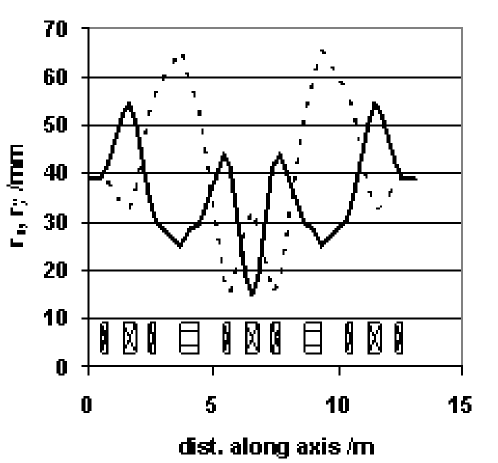
Figure 17: Beam radius $(r_{x},r_{y})$ along one arc of the APR lattice ($r_{x}$ – solid; $r_{y}$ – dashed).

The beam envelopes in the target section are shown in Fig 18, where a spot size of $r=10$ mm is required together with an angular divergence of 50 mrad.

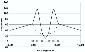
Figure 18: Beam radius $(r_{x},r_{y})$ around the gas target ($r_{x}$ – solid line, $r_{y}$ – dashed).

The phase space ellipse of the beam here is upright ($\alpha_{x,y}=0$).

In Fig. 19, the $\beta$–functions for the straight section provided for the electron cooling solenoid. Here $\beta_{x}=\beta_{y}=5$ m. Depending on the cross section of the electron beam $\beta_{x,y}$ can be adjusted to values between 1 and 10 m.

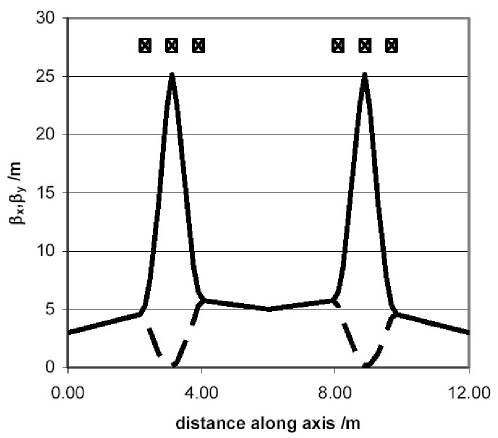
Figure 19: $\beta$–functions in the electron cooler section ($\beta_{x}$ – solid line, $\beta_{y}$ – dashed).

For the last section with Siberian snake and RF cavity, a wide variety of optical conditions may be realized with the foreseen quadrupoles. The same applies to the injection/ejection section.

8.5.4 Discussion of the APR Design

The APR lattice design presented here provides telescopic imaging through each of the 4 arcs of the ring. The quadrupole arrangements in the straight sections enable tuning of the beam within a wide choice of optical conditions. Plausible assumptions about the dimensions of the insertions have been made. The design of these insertions depends on the final lattice, and can be easily modified.

8.5.5 Realization of the APR based on Permanent Magnets

An important aspect concerning the realization of the APR concerns the employed conventional electromagnets (dipoles and quadrupoles). Since all APR magnets are set to a specific magnetic field or field gradient, the use of permanent magnets is an advisable alternative. For magnetic quadrupoles, the optical quality achieved so far with permanent magnetic material is excellent. Their great advantage would be:

1. Compactness of the quadrupoles,

2. savings in operational and investment costs, and

3. simple installation (neither power nor cooling water required).

A preliminary estimate for replacing the 72 conventional quadrupoles in this APR design with permanent ones leads to length reductions from 25 (50) cm to 10 (12) cm for the 2 families with a corresponding weight reduction from 220 (440) to 11 (31) kg. The reduced weight would also have profound implications for the support structure, alignment etc. The permanent quadrupole magnets would save operational power costs of 150 kW and the investment for water cooling. The design of dipoles with a specific bending strength employing permanent magnetic material is complicated, since they consist of an arrangement of circular slabs with appropriate spacing. A suitable design is under preparation and commercially available from the company UGS [149], which also offers the permanent magnet quadrupoles. Although details are not available at present, size and weight reductions for the dipoles are similar. The operation of the conventional dipoles would require a total power of 309 kW.

The antiproton polarizer, discussed here, would provide highly polarized antiproton beams of unprecedented quality. In particular the implementation of this option at the Facility for Antiproton and Ion Research would open new and unique research opportunities for spin–physics experiments in $\bar{p}p$ interactions at the HESR.

9 Cooler Synchrotron Ring CSR

The CSR has to accelerate polarized protons and antiprotons to momenta between 600 MeV/c and 3.65 GeV/c and is expected to be very similar to COSY [150]. A polarized ion source to provide a vector polarized proton beam is needed which is accelerated to about 50 MeV before injection into the CSR [151, 152]. The polarization is determined by measuring the asymmetry of $pC$ scattering from a carbon fiber target [153]. Additional polarimeters have to be installed after the LINAC to optimize the transition units in the polarized source for a high degree of polarization.

9.1 Injector LINAC for 50 MeV Polarized Protons

Low energy superconducting proton LINACs have been discussed recently as an optimum solution in terms of justifiable resources and available space. A layout for such a linac was worked out and proposed as a new injector for the COSY together with advanced ion sources and two interchangeable rf–quadrupoles (RFQ). It was designed to deliver both polarized and unpolarized pulsed H^-/D^- beams at a kinetic energy of  50MeV with a maximum repetition rate of 2Hz. The pulse length was limited to 500 ms and the beam current to 2 mA (peak). This compact design leads to a total LINAC length of less than 20 m. For producing the short pulses of high–intensity polarized H^-/D^- beams, a CIPIOS–type ion source like the one used at IUCF (Bloomington, Indiana) is suitable [154].

It should be noted that after the termination of the HERA program in 2007, the DESY proton LINAC might be available, which would also be a perfect CSR injector.

9.2 Acceleration of Polarized Proton and Antiproton Beam

In a strong–focusing synchrotron like the CSR two different types of strong depolarizing resonances are excited, namely imperfection resonances caused by magnetic field errors and misalignments of the magnets, and intrinsic resonances excited by horizontal fields due to the vertical focusing. In the momentum range of CSR, five imperfection resonances have to be crossed. Vertical correction dipoles or a weak partial snake of a few percentage can be utilized to overcome all imperfection resonances by exciting adiabatic spin flips without polarization losses. The number of intrinsic resonances depends on the superperiodicity of the lattice. In principle a typical magnetic structure of a synchrotron ring in this energy range allows to adjust superperiodicities of $P=2$ or even 6 like in COSY. However, due to symmetry–breaking modification of the interaction region and strong magnetic fields of detector magnets and the electron cooling system, a superperiodicity of $P=1$ is expected, leading to about ten intrinsic resonances. A tune–jump system consisting of fast quadrupoles has especially been developed to handle intrinsic resonances at COSY and will also be suitable for the CSR.

9.2.1 Imperfection Resonances

The imperfection resonances for polarized protons and antiprotons are listed in Table 6. They are crossed during acceleration, if the number of spin precessions per revolution of the particles in the ring is an integer ($\gamma G=k$, $k$: integer). The resonance strength depends on the vertical closed orbit deviation.

$\gamma G$	$E_{kin}$ (MeV)	$P$ (MeV/c)
2	108.4	463.8
3	631.8	1258.7
4	1155.1	1871.2
5	1678.5	2442.6
6	2201.8	2996.4

Table 6: Proton beam energies and momenta at which imperfection resonances occur in the CSR.

A solenoid with low magnetic field acting as a weak partial snake or vertical correction dipoles can be utilized in the CSR to preserve the polarization by exciting adiabatic spin flips. Both methods are successfully utilized in COSY and have the capability to overcome all imperfection resonances in the momentum range of the CSR.

9.2.2 Intrinsic Resonances

The number of intrinsic resonances depends on the superperiodicity $P$ of the lattice, which is given by the number of identical periods in the accelerator. CSR will be a synchrotron with a racetrack design consisting of two 180^∘ arc sections connected by straight sections. One straight section will be modified to allow interactions with the circulation beam in the HESR. In this case the superperiodicity of the ring will be one.

If the straight sections are tuned as telescopes with 1:1 imaging, giving a 2$\pi$ betatron phase advance, one then obtains for the resonance condition $\gamma G=k\cdot P\pm(Q_{y}-2)$, where $k$ is an integer and $Q_{y}$ is the vertical betatron tune. The corresponding intrinsic resonances in the momentum range of the CSR are listed in Table 7 for different superperiodicities $P$ and a vertical betatron tune of $Q_{y}=3.61$.

$P$	$\gamma G$	$E_{kin}$ (MeV)	$P$ (MeV/c)
1,2	$6-Q_{y}$	312.4	826.9
1	$-1+Q_{y}$	427.5	992.4
1	$7-Q_{y}$	835.6	1505.3
1,2	$0+Q_{y}$	950.7	1639.3
1,2,6	$8-Q_{y}$	1358.8	2096.5
1	$1+Q_{y}$	1473.9	2222.0
1	$9-Q_{y}$	1882.0	2659.4
1,2	$2+Q_{y}$	1997.1	2781.2
1,2	$10-Q_{y}$	2405.2	3208.9
1	$3+Q_{y}$	2520.3	3328.6

Table 7: Beam energy and momenta at which intrinsic resonances occur in the CSR for a working point $Q_{y}=3.61$, and superperiodicities of $P=1$, 2, and 6.

Intrinsic resonances in the CSR can be compensated by fast tune jumps with a similar system like in COSY. Due to symmetry–breaking installations like detector magnets and the arrangements for the interaction zone, the superperiodicity of the lattice is reduced to one, leading to ten intrinsic resonances. It has been proved that the tune–jump system of COSY can handle all ten intrinsic resonances in this momentum range. Therefore the same system is proposed for the CSR. Polarization measurements during acceleration confirm that the proposed concept allows the acceleration of a vertically polarized proton beam with polarization losses of only a few percent up to the maximum momentum of COSY. Therefore it is the ideal system for the CSR, which has very similar beam parameters.

10 PAX Requirements on the HESR Design

10.1 Introduction

For the Phase–II experimental program, polarized antiprotons stored in the HESR with energies up to 14.1 GeV are required. The APR–CSR system will provide antiprotons of up to 2.5 GeV. Therefore, polarized antiprotons have to be accelerated up to the highest HESR energies.

Instead of employing SIS 100 for acceleration, it appears to be much more economic to perform acceleration directly within the HESR. An efficient accumulation of polarized antiprotons in HESR, however, requires that at each cycle the remaining stack of polarized antiprotons is decelerated down to the injection energy and, after injection of additional antiprotons, is accelerated back to high energies.

Compared with the present HESR design [155], the following additional features are required:

• Acceleration using an rf–cavity,

• Slow ramping of the ring magnets,

• Stable spin during ramping and flat top by means of Siberian snakes,

• Spin manipulation of stored protons and antiprotons by means of rf–dipoles and solenoids,

• Injection of polarized antiprotons from CSR into the HESR, and

• Guiding the high–energy HESR beam to the PAX experiment in the CSR straight section by means of a chicane system.

10.2 Polarization Preservation

Acceleration and storage of polarized proton and antiproton beams in medium and high energy circular accelerator is complicated by numerous depolarizing spin resonances. In the following we discuss possible scenarios to accelerate and store polarized beams in the HESR.

The spin motion in an external electromagnetic field is governed by the so–called Thomas–BMT equation[156], leading to a spin tune of $\nu_{sp}=\gamma G$. In a strong–focusing ring like the HESR imperfection and intrinsic spin resonances can depolarize the beam.

10.2.1 Depolarizing Resonances

In total 25 imperfection resonances ranging from $\gamma G=4$ to $28$, and 50 intrinsic resonances from $\gamma G=16-Q_{y}$ to $16+Q_{y}$ for a vertical betatron tune of about $Q_{y}=12.2$ have to be crossed during acceleration. The corresponding imperfection and intrinsic resonances in the momentum range of the HESR for a vertical working point of $Q_{y}=12.14$ and superperiodicity $P=1$ are listed in Table 8

$\gamma G=...$	$\gamma G=...\pm Q_{y}$	$E_{kin}$ (GeV)	$P$ (GeV/c)
	16-	1.082	1.789
4		1.155	1.871
	-8+	1.228	1.953
	17-	1.605	2.364
5		1.678	2.443
	-7+	1.752	2.521
	18-	2.129	2.920
6		2.202	2.997
	-6+	2.275	3.073
	19-	2.652	3.465
7		2.725	3.541
	-5+	2.798	3.617
	20-	3.175	4.005
8		3.248	4.080
…	…	…	…
	15+	13.265	14.172
	40-	13.642	14.550
28		13.715	14.624
	16+	13.789	14.697

Table 8: Beam energy and momenta at which imperfection and intrinsic resonances occur in the HESR for a working point of $Q_{y}=12.14$.

The strength of the resonances depends on the orbit excursions for imperfection resonances and focusing structure of the lattice and beam emittance for intrinsic resonances and is ranging from $10^{-2}$ to $10^{-6}$ for the expected beam parameter. Due to coupling introduced by the 15 Tm solenoid of the Electron Cooler also strong coupling spin resonances are excited. The large number of resonances to be overcome in the HESR makes it very hard to apply techniques of individual manipulation of single spin resonances [157, 158, 159]. Siberian snakes seem to be to only option to guarantee a setup with low polarization losses during acceleration.

10.2.2 Siberian Snake with Combined Fields

In the HESR momentum range it is difficult use a RHIC–type [160] helical dipole snake due to large orbit excursions as shown in the upper left plot of Fig. 20.

Figure 20: Layout of a full Siberian snake with combined helical dipole and solenoidal magnetic fields.

A solenoidal field would require a pretty high integrated field strength of roughly 60 Tm. Therefore a magnet system with a combination of both field types was investigated, consisting of four RHIC–type helical dipole magnets with a maximum field of 2.5 T and a 15 Tm solenoid (see upper right plot in the same Figure). To provide a full spin flip in the whole momentum range the snake magnets have to be ramped according to the values given in the lower left plot, where $s$ is the solenoid and $d1,d2$ are the two helical dipole field values. The resulting spin motion at 15 GeV/c is shown in the lower right plot. This magnet system provides a full spin flip in the whole momentum range by keeping the maximum closed orbit excursion below 5 cm. Spin rotation induced by the DC Cooler solenoid at any possible field level can be compensated by the rampable 15 Tm snake solenoid, if snake and Cooler are installed in the same straight section.

10.2.3 Siberian Snake with Solenoidal Fields

The second proposed scheme contains four solenoids grouped on either side of the Cooler (see upper sketch of Fig. 21) with the same total integrated field strength of 15 Tm like the Cooler solenoid. From injection up to about 7.5 GeV/c all five solenoids will provide a full snake. At higher momenta they will work as partial snake with about $50\%$ partial snake at top momentum.

Figure 21: Layout of a Siberian snake with solenoidal fields (top) and optical functions (bottom).

To compensate for coupling, two groups of four quadrupole magnets are needed with rotation angles up to $8.6$, $6.3$, $4.3$ and $4.3$ degree. The rotation angles of the quadrupoles have to be adjusted for different solenoid fields and beam momenta. The whole magnet insertion provides a betatron phase advance of $\pi$ and $2\pi$ in the two transverse planes and has a total length of 56 m. To preserve polarization at first order spin resonances, the fractional part of the betatron tune has to be kept close to integer in the range $0.75<Q_{frac}<0.25$. This scheme does not excite orbit excursion and compensates for transverse phase space coupling. Applying higher integrated solenoidal field strength, it could also serve as a full Siberian snake.

The most serious drawback of a combined field scheme is large orbit excursion in the snake, which could be a major restriction for the beam quality in the HESR. Furthermore, ramping of the super–conducting snake magnets remains to be solved. Good field quality of the superconducting ring magnets is essential to apply a partial Siberian snake in order to keep the strength of higher–order spin resonances small combined with high flexibility of the lattice allowing for betatron tunes close to integer. A decision for one of the proposed schemes should be taken after intense particle and spin tracking including field errors and technical layout of the snake magnets.

10.3 Spin Manipulation of Polarized Protons and Antiprotons

Many polarized scattering experiments require frequent spin–direction reversals (spin–flips) during storage of the polarized beam to reduce their systematic errors. For maximum luminosity it is necessary to reverse the spins of the already stored antiprotons during the accumulation process, as was done in many IUCF experiments. Spin resonances induced by either an rf–solenoid or rf–dipole are well proven techniques to produce spin–flips in a controlled way. Spin flipping and spin manipulation of a stored beam was first studied in the IUCF Cooler Ring at 270 MeV [161]. In 2002, the SPIN@COSY collaboration was founded to continue these unique polarized beam studies in the GeV–regime at COSY [162]. Remarkably high measured proton spin–flip efficiencies of $99.92\pm 0.04\%$ were achieved by ramping the frequency of a strong ferrite–core water–cooled RF dipole through an rf–induced spin resonance at 2.1GeV/c [163]. The weak energy dependence of the spin–resonance strength induced by transversal rf fields indicates that only a slightly stronger rf dipole should allow efficient spin–flips of polarized antiprotons up to the maximum energy of the HESR.

10.4 Interaction Region Design for the Asymmetric Collider

To maximize luminosity, both the proton and the antiproton beam need to be focused to small spot sizes at the interaction point (IP) of the facility. Both beams also have to be separated close to the IP into their respective storage rings. Though a crossing angle would greatly simplify the interaction region design, luminosity loss due to the relatively long bunches makes it less desirable. We have therefore designed an interaction region for head–on collisions, where beams are magnetically separated, taking advantage of the unequal beam energies.

Due to the hourglass effect, the finite bunch length of some $30\,{\rm cm}$ results in a minimum reasonable $\beta$–function at the IP of $\beta^{\ast}=0.3\,{\rm m}.$ With normalized emittances of $\epsilon_{p,n}=1.7\pi\,\mu{\rm m}$ after cooling for the proton beam and $\epsilon_{\bar{p},n}=20\pi\,\mu{\rm m}$ for the antiproton beam and the requirement of equal beam sizes of both beams at the interaction point to avoid emittance blow–up of the larger beam due to the beam–beam effect, resulting $\beta$–functions at the IP are $\beta_{p}^{\ast}=0.3\,{\rm m}$ for the proton beam and $\beta_{\overline{p}}^{\ast}=1.0\,{\rm m}$ for the antiproton beam. Table 9 lists the design parameters of the interaction region.

bunch length $\sigma_{s}$	0.3 m
proton normalized emittance $\epsilon_{p.n}$	$1.7\pi\,\mu{\rm m}$
antiproton normalized emittance $\epsilon_{\overline{p}.n}$	$20\pi\,\mu{\rm m}$
proton $\beta^{\ast}$	$0.3\,{\rm m}$
antiproton $\beta^{\ast}$	$1.0\,{\rm m}$

Table 9: Parameter table.

With equal emittances in both transverse planes, the best beam–beam performance is obtained with round beams at the IP. The required equal $\beta$–functions in both planes are provided by low–$\beta$ quadrupole triplets near the interaction point. The quadrupoles for the low–energy proton beam are actually common to both beams; an additional vertical dipole field separates the two beams by deflecting the low–energy proton beam to a larger angle than the high–energy antiprotons. This field configuration is achieved by realization of those magnets as superconducting quadrupoles with additional dipole windings.

The low–$\beta$ triplet quadrupoles in the antiproton ring are designed as normal–conducting septum quadrupoles to minimize the required beam separation at the location of the first magnet. This configuration is schematically shown in Figure 22.

Figure 22: Schematic drawing of the interaction region configuration (top view).

Focusing for both beams is provided by quadrupole triplets. The shared superconducting low–$\beta$ magnets for the low–energy proton beam have peak fields of about $1.5\,{\rm T}$ for a beam pipe radius sufficient to provide a minimum aperture of $12\sigma$ for both beams, where $\sigma$ denotes the transverse rms beam size. Figure 23 shows the proton low–functions around the IP.

Figure 23: Proton low–$\beta$ lattice (one side only). Focusing is provided by a superconducting quadrupole triplet, starting at a distance of $3.0\,{\rm m}$ from the interaction point. The first and third magnet of the triplet are horizontally focusing, while the center quadrupole focuses in the vertical plane.

The normal–conducting septum quadrupoles for the high–energy antiproton beam have a peak field below $1.0\,{\rm T}$ for a minimum aperture of $12\sigma.$ The resulting $\beta$–functions are depicted in Figure 24.

Figure 24: Antiproton $\beta$–functions around the IP (one side only). Focusing is provided by a normal–conducting septum quadrupole triplet. The superconducting proton low–$\beta$ triplet on the left has only little effect on the antiproton optics due to the higher beam rigidity.

The septum itself is assumed to have a thickness of $5\,{\rm mm}$ in the horizontal mid–plane of the magnet. This is achieved by a triangular cut–out on the outside of the septum plate, which can be tolerated in terms of saturation since the magnetic field on the septum plate in the horizontal mid–plane of the magnet vanishes. Taking into account the wall thickness of the two beam pipes at the septum, the required separation of the two beams there is approximately

$$d = 12\sigma_{p}+12\sigma_{\overline{p}}+10\,{\rm mm}$$ (26)

$$= 67\,{\rm mm}.$$ (27)

This is achieved by a dipole field of $0.14\,{\rm T}$ over the total length of the superconducting quadrupoles.

With the parameters given in Table 9, the resulting beam–beam parameter

$$\xi=\frac{r_{p}}{4\pi\sigma^{2}}\cdot\frac{\beta^{\ast}}{\gamma}\cdot N$$ (28)

can be calculated. Here, $r_{p}$ denotes the classical proton radius, $\gamma$ the Lorentz factor of the beam under consideration, and $N$ the number of protons (antiprotons) per bunch. For $N=1.0\cdot 10^{11}$ protons and antiprotons, the resulting beam–beam tune shift is $\xi_{p}=6.25\cdot 10^{-3}$ for the proton beam and $\xi_{\overline{p}}=7.5\cdot 10^{-3}$ for the antiproton beam, which seems to be realistically achievable, based on experience at existing hadron colliders.

10.4.1 Luminosity Estimate for the Asymmetric Collider

The resulting luminosity for a single proton bunch colliding with three antiproton bunches of equal intensity of $N_{p}=N_{\overline{p}}=1.0\cdot 10^{11}$ particles yields

$${\cal{L}} = \frac{N_{p}N_{\overline{p}}f_{c}}{4\pi\sigma}$$ (29)

$$= 1\cdot 10^{30}\,{\rm cm}^{-2}{\rm sec}^{-1},$$ (30)

where $f_{c}$ denotes the bunch crossing frequency.

It should be emphasized here that in order to maximize luminosity the circumference ratio of the two storage rings needs to be reflected in the number of bunches circulating in each ring; hence the number of antiproton bunches needs to be three times larger than the number of proton bunches.

10.4.2 Intensity dependent Limitations

Due to the high bunch charge of $N=1.0\cdot 10^{11}$ particles per bunch in conjunction with low beam energies, intensity dependent effects need to be studied carefully. Here we list some estimates of high intensity effects that are to be expected at the proposed facility.

10.4.2.1 Touschek Lifetime

Single scattering of particles within the same bunch leads to momentum transfer from the transverse into the longitudinal plane, where particles get lost if their longitudinal momentum exceeds the momentum acceptance of the machine. The resulting Touschek lifetime is expressed as [164]

$$\tau_{\rm Touschek}^{-1} = \frac{Nr_{p}^{2}c}{8\pi\sigma_{x}\sigma_{y}\sigma_{s}}\cdot\frac{\left(\frac{\Delta p}{p}\right)^{-1}}{\gamma^{2}}\cdot D(\xi).$$ (31)

Here, $r_{p}$ denotes the classical proton radius, while $c$ is the velocity of light. The function $D(\xi)\approx 0.3$ for realistic parameter ranges [164]. Assuming a momentum acceptance of $\Delta p/p=0.01$ and using average values of $\sigma_{x}=\sigma_{y}=3.5\,{\rm mm}$ and $\sigma_{s}=0.3\,{\rm m}$ for the transverse and longitudinal rms beam sizes, respectively, this yields a Touschek lifetime exceeding a year. This effect is therefore of no concern for the facility.

10.4.2.2 Intrabeam Scattering

Multiple scattering of particles within the same bunch, also called intrabeam scattering, leads to emittance growth in all three dimensions. Growth rates are calculated as [164]

$$\frac{1}{T_{p}} = \left\langle A\frac{\sigma_{h}^{2}}{\sigma_{p}^{2}}f(a,b,q)\right\rangle,$$ (32)

$$\frac{1}{T_{x}} = \left\langle A\left[f\left(\frac{1}{a},\frac{b}{a},\frac{q}{a}\right)+\frac{D_{x}\sigma_{h}^{2}}{\sigma_{x\beta}^{2}}f(a,b,q)\right]\right\rangle,$$ (33)

$$\frac{1}{T_{y}} = \left\langle A\left[f\left(\frac{1}{b},\frac{a}{b},\frac{q}{b}\right)+\frac{D_{y}\sigma_{h}^{2}}{\sigma_{y\beta}^{2}}f(a,b,q)\right]\right\rangle,$$ (34)

with

$$A = \frac{r_{p}^{2}cN}{64\pi^{2}\beta^{3}\gamma^{4}\epsilon_{x}\epsilon_{y}\sigma_{s}\sigma_{p}},$$ (35)

$$\frac{1}{\sigma_{h}^{2}} = \frac{1}{\sigma_{p}^{2}}+\frac{D_{x}^{2}}{\sigma_{x\beta}^{2}}+\frac{D_{y}^{2}}{\sigma_{y\beta}^{2}},$$ (36)

$$a = \frac{\sigma_{h}\beta_{x}}{\gamma\sigma_{x\beta}},$$ (37)

$$b = \frac{\sigma_{h}\beta_{y}}{\gamma\sigma_{y\beta}},$$ (38)

$$q = \sigma_{h}\beta\sqrt{\frac{2d}{r_{p}}}.$$ (39)

$\epsilon_{x}$ and $\epsilon_{y}$ denote the horizontal and vertical emittance, respectively, while $d$ is the smaller of the horizontal and vertical rms beam sizes.

Using the beam emittances given in Table 9, $\sigma_{p}=1.0\cdot 10^{-3},$ and average $\beta$–functions $\beta_{x}=\beta_{y}=30\,{\rm m},$ the value of the function $f(a,b,q)$ can be obtained from Ref. [164] as $f(a,b,q)\approx-100.$ This yields a longitudinal emittance growth rate of

$$T_{p}^{-1}\approx 10^{-3}\,{\rm sec}^{-1},$$ (40)

and results of similar magnitude for the transverse rates $T_{x}^{-1}$ and $T_{y}^{-1},$ which is comparable to the design cooling times. This is a major concern for the proposed facility and requires a thorough investigation, taking into account the actual accelerator lattices.

11 Polarimetry

The beam and target polarization will be determined by the following scheme: First the target polarization using an unpolarized antiproton beam is established by either one of two methods:

• with reference to a suitable sampling polarimeter of the Breit–Rabi [165] or Lamb–shift [166] type, which spin–analyzes a small fraction of atomic hydrogen extracted from the target cell.

• elastic proton–antiproton scattering data at low energies (500–800 MeV) where analyzing power data from PS172 [167] are available. Scattering data of lower precision extend up to 2.5 GeV [168].

This allows one to calibrate a suitable detector asymmetry, derived from elastic scattering, in terms of an effective analyzing power. Since target and beam analyzing power in $\bar{p}p$ scattering are identical, the polarization of the beam can now be measured with an unpolarized target (e.g. by injecting unpolarized hydrogen gas into the cell). When subsequent fills of the HESR are made with different beam energies, it is straightforward to establish polarization standards at any energy within the HESR range by exploiting the fact, that the target polarization is constant with time – or monitored by the sampling polarimeter – and independent of energy [169].

Part III Staging of Experiments

The PAX collaboration proposes an approach that is composed of different stages. During these the major milestones of the project can be tested and optimized before the final goal is approached: a polarized proton–antiproton asymmetric collider, in which about 3.5 GeV/c polarized protons will collide head–on with polarized antiprotons with momenta up to 15 GeV/c.

12 Preparatory Phase

12.1 Accelerator: Design and Construction of the Antiproton Polarizer Ring

Tuning and commissioning of the APR will require a beam of polarized protons. Such a beam and a hall including infrastructure are readily available at COSY–Jülich. This makes Institut für Kernphysik of the Forschungszentrum Jülich the ideally suited site for the design, construction and testing of the APR.

12.2 Physics in the Preparatory Phase

The calculation of the polarization transfer employed to polarize the antiprotons is text book QED physics [170]. The polarization transfer technique is at the core of an extensive physics program at JLAB dedicated to experiments on the separation of the charge and magnetic form factors of the proton [126]. The existence of the effect has been verified in the FILTEX experiment at TSR–Heidelberg in 1992 with a 23 MeV proton beam. For antiprotons the optimal energy is around 50 MeV (see Sec. 8.3). We don’t consider necessary a further demonstration of the validity of this fundamental QED derivation and, unless specifically requested by the QCD–PAC, we would not embark on such endeavor. Instead, we would very much prefer to concentrate on the design, construction, commissioning and direct proof with the APR that protons can be polarized to a high degree with a design energy of 50 MeV. If however, the QCD–PAC will ask us for a pre–APR test, this can be carried out at COSY.

• A verification of $\sigma_{EM_{\perp}}$ at 40, 70 and 100 MeV is possible using the polarized internal target at the ANKE interaction point.

  The measurement can be performed by injecting pure states $\left|\,1\,\right>$ or $\left|\,3\,\right>$ in a weak transverse target guide field (10 G). In this situation the electron target polarization $Q_{e}$ is equal to the proton target polarization $Q_{p}$ and $Q_{p}$ can be measured by $pp$ elastic scattering by using the ANKE spectator detector system [171].

12.3 Development of Polarized Sources

The polarization mechanism relies on an efficient, high–intensity source for polarized hydrogen atoms. In the PAX collaboration, most of the world–expertise on polarized sources is already present (Erlangen, Ferrara, Gatchina, Jülich, Madison). A program for the development of a new generation of high–intensity atomic beam sources has been already started in Ferrara and it will be pursued and extended during the preparatory phase of the PAX experiment.

13 Phase–I

13.1 Accelerator: Transfer of APR and CSR to FAIR

APR and CSR will be placed inside the HESR. The straight sections of CSR and HESR are parallel, whereby an additional IP, independent of the PANDA IP, is formed.

13.2 Physics in Phase–I

A beam of unpolarized or polarized antiprotons with momentum up to 3.5 GeV/c in the CSR ring, colliding on a polarized hydrogen target in the PAX detector will be available. This phase is independent of the HESR performance. This first phase, at moderately high–energy, will allow for the first time the measurement of the time–like proton form factors in single and double polarized reactions from close to threshold up to 3.5 GeV/c. It will be possible to determine several (single and double) spin asymmetries in the elastic $p\bar{p}\to p\bar{p}$ process. By detecting back scattered antiprotons one can also explore hard scattering regions of large $t$: in the proton–proton scattering reaching the same region of $t$ requires a twice higher energy. This would allow us to carry out the measurements of form factors with a fixed polarized hydrogen target bombarded by antiprotons orbiting in the CSR with momenta of 3.5 GeV/c. The CSR would be fed with antiprotons from the APR.

14 Phase–II

14.1 Accelerator: HESR modifications to collider mode or to polarized internal target.

A chicane for CSR and HESR has to be built to bring the proton beam of the CSR and the antiproton beam of the HESR to a collision point at the PAX IP.

14.2 Physics in Phase–II

This phase will allow the first ever direct measurement of the quark transversity distribution $h_{1}$, by measuring the double transverse spin asymmetry $A_{TT}$ in Drell–Yan processes $p^{\uparrow}\bar{p}^{\uparrow}\rightarrow e^{+}e^{-}X$ as a function of Bjorken $x$ and $Q^{2}$ (= $M^{2}$). Two possible scenarios might be foreseen to perform the measurement.

• A beam of polarized antiprotons from 1.5 GeV/c up to 15 GeV/c circulating in the HESR, colliding on a beam of polarized protons of 3.5 GeV/c circulating in the CSR. This scenario requires to demonstrate that a suitable luminosity is reachable. Deflection of the HESR beam to the PAX detector in the CSR is necessary (see Fig. 9). By properly varying the energy of the two colliding beams, this setup would allow a measurement of the transversity distribution $h_{1}$ in the valence region of $0.1<x<0.8$ with corresponding $Q^{2}$ in the range $4<Q^{2}<100$ $\rm GeV^{2}$ (see Fig. 1). $A_{TT}$ is predicted to be larger than 0.2 in the full kinematic range, see Fig. 1, and the cross section is large enough to get $\sim 2000$ events per day at a luminosity of $5\cdot 10^{30}$ $\rm cm^{-2}s^{-1}$. Such an experiment can be considered, for $h_{1}$, the analogous of polarized DIS for the helicity distribution $\Delta q$; the kinematical coverage in $(x,Q^{2})$ will be similar to that of the HERMES experiment.

• Should the requested luminosity for the collider not be reachable, a fixed target experiment can be performed. A beam of 22 GeV/c (15 GeV/c) polarized antiprotons circulating in the HESR, can be used to collide on a polarized internal hydrogen target. Also this scenario requires the deflection of the HESR beam to the PAX detector in the CSR (see Fig. 9). A theoretical discussion of the significance of the measurement of $A_{TT}$ for a 15 GeV/c beam impinging on a fixed target is given is Refs. [2] and [3] and the recent review paper [11]. This measurement will explore the valence region of $0.3<x<0.8$ with corresponding $4<Q^{2}<16$ ${\rm GeV}^{2}$, see Fig. 1. In this region $A_{TT}$ is predicted to be large (of the order of 0.3, or more) and the expected number of events can be of the order of 2000 per day.

Part IV Detector

15 Requirements and Design Considerations

Since a definite choice has not been made yet on the accelerator configuration (fixed target or collider), it might be premature at this stage to define the detector details. Still some general considerations can be anticipated. What we present here is just meant as a conceptual detector design suitable for the PAX physics program. Possible alternative scenarios will be discussed at the end in Sec. 19.

In the following we focus on the most challenging task of the PAX physics program: the measurement of the Drell–Yan reaction to access the transversity distribution $h_{1}$. A detector optimized for this task can be designed to be suitable to achieve also the other goals of the PAX experimental program.

In the detector concept, presented below, the following criteria have been pursued:

• optimize the acceptance at large angles. The double spin asymmetry of the $q\bar{q}\to\ell^{+}\ell^{-}$ QED elementary process,

  $$\hat{a}_{TT}={\sin^{2}\theta\over 1+\cos^{2}\theta}\>\cos 2\phi\,,$$ (41)

  maximizes the sensitivity of the measured asymmetry $A_{TT}$ for the transversity distribution $h_{1}$ for 90–degree scattering in the center–of–mass of the partonic system, where $\sin^{2}\theta\sim 1$ (see Eq. (1). We note that also the $\overline{p}p$ elastic scattering at 90^∘ c.m. and the form–factor measurements benefit from a large angle detector;

• trigger efficiently on the rare Drell–Yan events. At the PAX energy the few nb Drell–Yan cross section should be clearly identified from a total $\overline{p}p$ cross–section of about 50 mb;

• cope with the overwhelming background. The lepton identification should provide a rejection factor of the order of $10^{4}$ to $10^{5}$ against hadrons. Secondary leptons, produced in meson decays and in secondary interactions in the detector material, should be vetoed as well;

• provide of the order of 1 % resolution for the invariant mass of the lepton pairs, in order to efficiently distinguish the contribution of the resonances ($J/\Psi$ and $\psi$) from the continuum;

• (if the collider option would be pursued) be compatible with the asymmetric collider lattice. In particular any effect of the spectrometer magnet should be perfectly compensated in order to not degrade the beam polarization;

• provide a unique facility as complete as possible and flexible to allow the study of auxiliary processes and additional physical channels which might become interesting during the next 10 years.

In order to best match the above requirements, the PAX detector is designed to measured electron–positron pairs of large invariant mass.

15.1 Physical Channels

To reveal rare reactions like the Drell–Yan process and the $\overline{p}p\rightarrow e^{+}e^{-}$ annihilation, the PAX detector has to be conceived as a large acceptance apparatus capable of unambiguously identifying electron–positron pairs of large invariant mass and precisely measuring their momenta. The detector has to be able to measure electron pairs with large opening angle, in a wide kinematic range with good angular and energy resolution. A clear particle identification is required to separate the electrons of the wanted processes from the large pion background.

Reactions characterized by two–body hadronic final states like elastic scattering, present a higher cross–section and put less stringent constraints on the detector design. They can be identified by measuring scattering angles and momenta of the hadronic particles by employing coplanarity and total momentum conservation. Finally, the PAX detector can measure the energy of gammas from radiative processes and $\pi^{0}$ and $\eta$ decays.

15.2 Particle Identification

The Drell–Yan production rate is of the order of $10^{-7}$ of the total $\overline{p}p$ reaction rate and results in a low yield of the $e^{+}e^{-}$ signal per interaction. In order to maximize the dilepton detection efficiency, the PAX spectrometer must provide a large geometrical acceptance. At the same time, the high interaction rate (of the order of 10⁶ s^-1) together with the hadron multiplicity represents a serious challenge to the trigger system which has to select the events containing the lepton tracks. An accurate lepton identification can only be achieved by detectors which are highly insensitive to the large flux of hadrons. In order to minimize the background from lepton misidentification at a typical prevailing $e/\pi$ ratio of $10^{-4}$, redundant recognition of lepton tracks is essential. For the considered range of momenta (between $0.5$ and $10$ GeV/c) electrons offer the advantage with respect to muons of that they can be identified in a hadron blind gas threshold Čerenkov detector. This device can be operated on a fast time scale to meet the stringent trigger requirements in the high–rate high–multiplicity environment. Additional discrimination against pions can be provided both by the cluster lateral profile in the electromagnetic calorimeter (CAL) and by the $E/p$ ratio between the energy $E$ measured in the CAL and the momentum $p$ measured in the spectrometer. With these constraints, the required rejection factor of the order of $10^{10}$ against hadronic events (corresponding to $10^{5}$ for single track events) is achievable, as demonstrated in other experiments [172, 173].

15.3 Magnetic Field Configuration

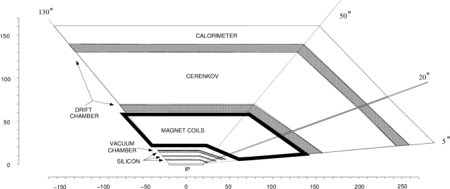
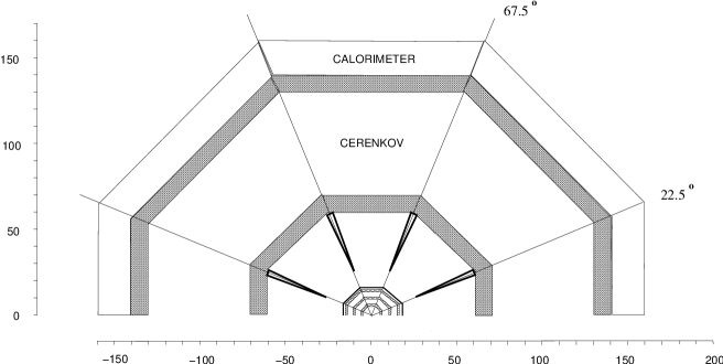
Figure 26: Sketch of the PAX detector, showing a side view ([$z,y$], top) and a view in beam direction ([$x,y$], bottom). The optional forward detector, sensitive at laboratory polar angles between $5^{\circ}$ and $20^{\circ}$, is also indicated.

The spectrometer magnet has to be compatible with the Čerenkov detector which needs to work in a field free region. A toroid configuration satisfies this requirement resulting in a negligible fringe field both along the beam line and external volume where the Čerenkov detector is located. A toroid field is always orthogonal to the particle momentum, hence the bending effect is optimized regardless of the scattering angle. An eight–coil configuration can be designed to give excellent coverage over the azimuthal angles, facilitating the detection of the $\cos(2\phi)$ modulation of the transverse asymmetry, covering the region around $2\phi=n\pi$, where the sensitivity is largest (see Fig. 26). The azimuthal acceptance is optimized by placing service and support structures of the various detectors in the shadow of the toroid coils. The detectors are arranged in an azimuthally eight–fold segmented, frustum–like geometry. For compactness, the inner tracking close to the interaction point is provided by silicon strip detectors. The outer tracking, behind the magnet, is provided by two sets of conventional drift–chambers. The Čerenkov detector is placed outside the magnet, in between the two sets of drift–chamber, fitting the $0.6-0.8$ m tracking arm required to obtain the $\sim 1$ % momentum resolution with a typical spatial resolution of $\sim 200$ $\mu$m.

15.4 Mass Resolution

A lepton pair invariant mass resolution close to 1 % is required to isolate the charmed resonance signals from the continuum. This value necessitates that the momentum resolution is of the same order of magnitude for lepton tracks with a momentum range between 0.5 and 10 GeV/c. This large momentum range leads to a non–focusing geometry with a transverse momentum kick up to $\Delta p\sim 0.3$ GeV/c. The maximum value of $\Delta p$ is required in the forward region where the particle momenta are larger and is provided by an integrated field along the particle trajectory of $Bl\sim 1$ Tm. In order to limit the cost of the external electromagnetic calorimeter, the detector should be compact: by assuming a value of $l=0.7$ m in the forward direction, the required magnetic field is of the order of 1.5 T. A transverse momentum kick of $\Delta p\sim 0.3$ GeV/c puts constraints on the position resolution of the tracking detectors to achieve the required momentum resolution. At a momentum of 10 GeV/c, the deflection angle equals about $2^{\circ}$. A model calculation shows that an uncertainty in the position lower than $30$ $\mu m$ ($200$ $\mu m$) in the inner (outer) tracking region is needed to obtain a relative momentum resolution of about 1 %. This resolution can be provided by conventional silicon strip detectors (SiD) close to the target and drift–chamber modules (DCH) outside the magnet. The high spatial resolution provided by the silicon detector will help to identify the background leptons from secondary vertex (like $D^{\pm}$ decays). The required momentum resolution can only be achieved by keeping multiple scattering in the magnetic field region small. If only multiple scattering is taken into account, the momentum resolution of $\sim 1$ % at the smallest accepted momenta of $0.5$ GeV/c requires an effective thickness less than $0.05$ $X_{0}$. The amount of material in the tracking region should be minimized also to reduce the gamma conversion probability and energy loss by radiation. The first active tracking layers placed inside the target vacuum chamber can be used to veto gamma conversions as close as possible to the interaction point.

15.5 General Remarks

The present conceptual detector design is based on existing experiments which have been proven to perform well measuring final–state particles and energies similar to the ones anticipated at PAX.

Once the PAX experiment is approved, each of the detector components will be further optimized depending on the chosen beam configuration. The performance of the detectors will finally depend (and benefit) from the development in technology over the course of the next ten years. Additional detectors can also be implemented to enhance the flexibility of the PAX instrument. As an example, hadron identification at forward scattering angles could be considerably improved by adding an internally–reflecting ring–imaging Čerenkov detector [174].

The PAX detector will be mounted on a platform which can be moved on rails in and out of the beam line. For simplicity, in the following we will refer only to Drell–Yan processes, the argument holds for $J/\Psi$ decays and time–like electromagnetic form factors as well.

16 Overview of the PAX Spectrometer

The PAX large–acceptance spectrometer (LAS) (Fig. 25) is optimized to detect electromagnetic final states with two charged tracks of high invariant mass.

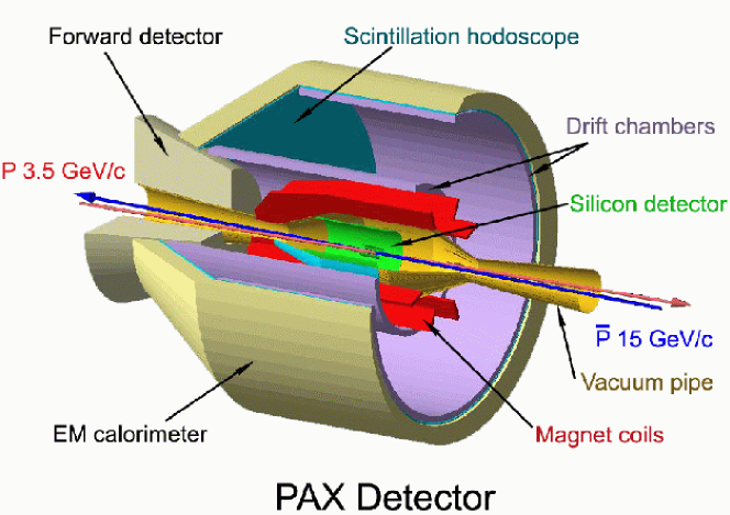
Figure 25: Artists view of the PAX spectrometer.

A clear identification of electrons is required to separate scattered electrons of the Drell–Yan mechanism from the large $\pi$ background. The detector is designed to also detect two–body hadron reactions using kinematical constraints, i.e. coplanarity and total momentum conservation. Moreover it can measure the energy of gammas from radiative processes and $\pi^{0}$ and $\eta$ decays.

The very inner part of the detector is devoted to triggering and tracking of charged particles. The scattering angles as well as the initial trajectory for the determination of the particle’s momentum are measured by a vertex tracking system consisting of three layers of double–sided silicon strip detectors (SiD). The momentum measurement is completed by two sets of drift chambers behind the magnet (DC). A possible additional set of drift chambers inside the magnet (MC) would improve the matching between the inner and outer tracks and help to resolve multiple tracks and to identify gamma conversions. This will allow us to detect low–momentum tracks which do not reach the external section of the spectrometer.

A threshold Čerenkov counter (CER) provides trigger capability for electrons and positrons produced in Drell–Yan processes. Electron and photon energies and directions are measured by the CAL. Both the CER and the CAL provide fast response and can be employed in the selection of electromagnetic particles to obtain a $\pi/e$ rejection factor $\lesssim$ 100 at trigger level and larger than $10^{4}$ in the off–line analysis for a single track. A pre–shower detector (PS) can possibly be added in front of the calorimeter to improve the pion rejection and the resolution on the impact point of photons. The outermost set of drift chambers can be filled with Xe–methane gas and can be complemented by a radiator to provide an additional $\pi$ rejection through transition radiation detection.

The central detector is designed to assure full acceptance between $\pm 20^{0}$ and $\pm 130^{0}$ for polar angles in the laboratory frame. It is not active in the small sectors of azimuthal angles in correspondence of the toroid coils. In these sectors the service systems for the detectors and the support structure of the system can be mounted. In the present design, no real limit exists for the maximum acceptable polar angle: the above values can be taken as indicative for the collider option and can be easily adapted to match different beam configurations. The detectors point toward the central part of the interaction region in a projective geometry.

An internal reflecting ring–imaging Čerenkov counter (DIRC) can be employed to identify charged hadrons (pions, kaons and protons). This provides flavor separation in single–spin asymmetry investigations, as well as in the analysis of other semi–inclusive and exclusive channels. The CAL allows the reconstruction of neutral pions in the hadronic final state. CER and CAL are included in the trigger together with a first hodoscope placed in front of the magnet and a second one before the calorimeter.

16.1 Toroid Magnet

The toroid magnet consists of 8 coils symmetrically placed around the beam axis. A support ring upstream of the target hosts the supply lines for electric power and for liquid helium. At the downstream end, an hexagonal plate compensates the magnetic forces to hold the coils in place. The field lines of an ideal toroid magnet are always perpendicular to the path of the particles originating from the beam line. Since the field intensity increases inversely proportional to the radial distance: greater bending power is available for particles scattered at smaller angles, which have higher momenta. These properties help to design a compact spectrometer that keeps the investment costs for the detector tolerable. The production of such a field requires the insertion of the coils into the tracking volume shadowing part of the azimuthal acceptance. Preliminary studies show that the use of superconducting coils, made by a $\rm Nb_{3}Sn$–Copper core surrounded by a winding of Aluminum for support and cooling, allows one to reach an azimuthal detector acceptance in excess of 80%, while the radius of the inner tracking volume can be kept below 0.7 m.

16.2 Silicon Detector

Three layers of double–sided silicon strip detector provide a precise vertex reconstruction and tracking of the particles before they reach the magnet. The design is based on the vertex detector of BABAR [174], with a smaller number of silicon layers to minimize the radiation length of the tracking material. The read–out electronic can be mounted in the front and back parts of the detector, outside the acceptance of the spectrometer. With a pitch of $50-100$ $\rm\mu m$ it is possible to reach an intrinsic spatial resolution of $10-20$ $\rm\mu m$. Such a spatial resolution should allow one to partially resolve and reject the secondary decays of $D^{\pm}$ mesons into leptons. Due to the associated production of charmed mesons, this kind of background can not be completely eliminated by subtracting the dilepton events with the same charge. The number of channels required to cover the 40 cm long interaction point is of the order of $2\cdot 10^{5}$, comparable with the BABAR experiment [174].

16.3 Drift Chambers

The required position resolution of $200$ $\mu$m after passage through the magnetic field can be achieved using conventional drift chambers [175, 176]. On the basis of an existing set–up [175], the chambers are assembled as modules consisting of four pairs of tracking planes with wires at $-30^{\circ},\,0^{\circ},\,0^{\circ},+30^{\circ}$ with respect to the direction transverse to the plane of the coil, i.e. parallel to the magnetic field lines. The wires of the planes oriented at $0^{\circ}$ are staggered in order to resolve left–right ambiguities. Uniform arrays of cathode wires separate the different cell layers. The tilted angles are optimized to provide a two–dimensional hit–point with emphasis on the polar (bending) coordinate. The support structure of the wires, together with the feedthroughs and the circuit boards for sector pairs, can fit within the shadow of the coils [176]. With a cell size of 0.5 cm, the total number of channels is about 32000. The expected momentum resolution is of the order of $1$ % over the kinematic range of the experiment.

16.4 Čerenkov Detector

A threshold gas Čerenkov counter is used to trigger and select electrons in the presence of a large hadronic background. The required background event reduction at trigger level is of the order of $10^{3}$, and is achieved with a $\pi/e$ rejection factor of $\lesssim 100$ on the single charged particle. The counter occupies a $60-80$ cm thick shell around the inner tracking detector and is divided into eight identical azimuthal sectors. Each sector can be further subdivided into s small number of gas cells. In this way the gas filling of each cell can be optimized cover the momentum range of interest by exploiting the correlation between scattering angle and particle momentum [177]. Freon–12 and $\rm CO_{2}$ are suitable gases for the energies involved in the PAX experiment [177, 178]. Čerenkov photons are reflected by aluminized carbon–fiber mirrors towards photomultipliers that can be located outside of the spectrometer acceptance within the shadow of the toroid coils [179]. The spatial resolution in the polar angle can be enhanced by segmenting the mirror and focalizing the light onto a row of photomultipliers [179]. A solution with multi-wire proportional chambers as photon detector with a solid CsI cathode pad is under study to obtain a higher spatial resolution [180].

16.5 Calorimeter

The calorimeter consists of radiation–resistant lead tungstate ($\rm PbWO_{4}$) crystals which have been selected for their high density, short radiation length and small Moliere radius. Unlike the CMS [181] and ALICE [182] experiments, the PAX calorimeter is not immersed inside a high magnetic field. This makes the use of photomultiplier tubes possible, to provide less noise and better resolution at low energies. The crystals are arranged in a barrel and in a conically–shaped endcap of the experiment in a quasi–projective geometry. They are supported from outside to minimize the material preceding the active region. The blocks have an area of $4\times 4\,\rm cm^{2}$ and a variable length matching the mean momentum of the impinging particles. The expected energy resolution can be parameterized as $\sigma(E)/E[\%]=1.8/\sqrt{(E[{\rm GeV}])}+0.4$ [183]. For the conditions at PAX this translates into an energy resolution of $2-3$ %. The calorimeter is used to trigger on Drell–Yan electrons by selecting the events with energy deposited in two clusters, both with a corresponding positive Čerenkov signal, which have large invariant mass. A back–to–back topology and a total deposited energy equal to the center–of–mass energy can be required to trigger on $\overline{p}p\rightarrow e^{+}e^{-}$ annihilation events. Assuming an electron identification efficiency of 90 %, a hadron rejection factor of several hundreds can be achieved by using the lateral profile of the deposited energy and the $E/p$ ratio between energy $E$ deposited in the calorimeter and the momentum $p$ measured in the spectrometer. The estimated number of crystals in the calorimeter is about 15000.

16.6 Hodoscopes

Two hodoscope planes are used for triggering together with CAL and CER detectors. A front trigger scintillator is placed directly upstream of the vacuum chamber. It consists of eight–fold segmented foils of standard plastic scintillator, 3.2 mm thick (0.7 % radiation length), read–out by phototubes. A second scintillator hodoscope is placed in front of the calorimeter. The counter is composed of modules of fast scintillators with a large attenuation length (300–400 cm). The modules are longitudinally oriented providing a barrel geometry. The scintillation light is detected by photomultiplier tubes. To provide additional particle identification, a passive Pb radiator (2 radiation lengths) can be placed in front of the external hodoscope to initiate electromagnetic showers that deposit typically much more energy in the scintillator than minimum–ionizing particles.

16.7 Forward Spectrometer

A forward spectrometer (FS) covering scattering angles below 20^∘, is envisaged to complement the LAS during data–taking at high energy. The tracking system of the forward spectrometer has the same design as the central one, and will benefit from the large field integral of the toroidal magnet at small angles (where the coils are closer each other).

The particle identification of the forward spectrometer has to be adapted to the chosen beam configuration. The sensitivity on the transverse distribution $h_{1}$ in the forward direction is poor, because $\hat{a}_{TT}$ is small there. In the asymmetric collider mode, Drell–Yan events with scattering angles below $20^{\circ}$ in the laboratory frame basically do not improve the statistical precision of the $h_{1}$ measurement. The forward region will be crucial for the SSA measurements at high energy and large values of $x_{F}$, so that the forward particle identification has to be optimized for hadrons. One promising option is to make use of a RICH detector [184]. For a fixed–target experiment with 22 GeV/c beam momentum, the lower limit of the useful scattering angle reduces to $5^{\circ}$ due to the relativistic boost. The PID of the FS has to be optimized for electron detection like the LAS.

16.8 Recoil Detector

A silicon recoil detector system is needed for the low–$t$ antiproton–proton elastic scattering program and will only be installed for these measurements, so that radiation damage will be a minor issue.

Figure 27: (a) Laboratory kinetic energy (top) and scattering angles (bottom) of the recoil proton for three different beam momenta. (b) Cross sectional view of the recoil detector.

At very low momentum transfer ($|t|=0.002\ldots 0.02$ GeV²) the recoil protons are detected by silicon strip detectors close to 90^∘ laboratory angle. At these angles (cf. Fig. 27a) the protons of interest have energies between 1 and 10 MeV and are stopped in a telescope comprised of a 65 $\mu$m thin surface barrier detector and a 1 mm thick microstrip detector. Such a telescope [171] has already been successfully operated in a similar environment at the ANKE experiment at COSY/Jülich. In view of the comparably large cross section (${\rm d}\sigma/{\rm d}t>150$ mb/GeV²) a precise measurement of the recoil energy is sufficient both to determine $t$ and to cleanly identify elastically scattered protons as in the E760 experiment at FNAL [185].

Four of these detectors cover azimuthal angle intervals of $\Delta\phi\approx 50^{\circ}$ in four quadrants, sketched in Fig. 27 (b). The acceptance is matched to the central part of the interaction region (collider mode) or of the storage cell (fixed–target mode). For the fixed–target Phase–I at moderately high energies, dedicated cell walls can be made as thin as 5 $\mu$m Teflon – as demonstrated by the PINTEX–experiment at IUCF [186] – and allow the detection of recoil protons down to about 500 keV kinetic energy. However, the low recoil momenta prohibit the use of a strong target guide field, such that measurements must be taken with a single pure hyperfine state and a weak (some mT) guide field to avoid strong bending of the recoils at very low $t$. The toroid magnet of the spectrometer provides a field free region around the interaction point and does not disturb the recoil trajectory.

The spin–dependent cross section $\frac{{\rm d}\sigma}{{\rm d}t}$ for vertical beam polarization $P_{y}$ and a transverse target polarization $Q_{x}$, or $Q_{y}$ is given by

$$\begin{array}[]{rcl}\frac{{\rm d}\sigma}{{\rm d}\Omega}(\vec{P},\vec{Q},\theta,\phi)=\left.\frac{{\rm d}\sigma}{{\rm d}\Omega}\right|_{\rm unpol.}\left(1\right.&+&\left[(P_{y}+Q_{y})\cos\phi+Q_{x}\sin\phi\right]A_{\rm N}\\ &+&P_{y}Q_{y}\left[A_{\rm NN}\cos^{2}\phi+A_{\rm SS}\sin^{2}\phi\right]\\ &+&\left.P_{y}Q_{x}\left[A_{\rm SS}-A_{\rm NN}\right]\sin\phi\cos\phi\right)\\ \end{array}$$ (42)

which relates by integration over $\phi$ and change of variables to the differential cross section difference

$$\frac{{\rm d}\Delta\sigma_{T}}{{\rm d}t}=-\frac{{\rm d}\sigma}{{\rm d}t}\left(A_{\rm NN}(t)+A_{\rm SS}(t)\right)$$ (43)

with $\Delta\sigma_{T}=\sigma\left(\uparrow\downarrow\right)-\sigma\left(\uparrow\uparrow\right)$. With this experiment spin correlation parameter $A_{NN}$, $A_{SS}$ as well as the analyzing power $A_{N}$ of $\bar{p}p$ elastic scattering are accessible.

16.9 Trigger and Data Acquisition

The actual interaction rate achievable by the PAX experiment will be precisely estimated only after the final beam configuration is known. However, an upper limit is anticipated to be of the order of a few MHz. A reduction factor of $10^{3}$ at trigger level is then required to keep the rate of read–out events below a few kHz.

For the different physics issues to be studied, dedicated trigger schemes have to be employed. The detection of Drell–Yan electron pairs will be accomplished by using coincidences comprising multiplicity information from the hodoscopes, silicon detectors, CAL and segments of the Čerenkov counter in the LAS. For single–spin asymmetries a single–prong trigger, derived from the forward scintillator hodoscopes and the calorimeter, can be used in a similar way as in the HERMES experiment [187]. For the low–$t$ elastic antiproton–proton scattering the recoil–detector hodoscope provides self–triggering capability for low energy hadrons, as demonstrated at ANKE [171].

High luminosity (above $10^{32}$ cm^-2s^-1 in the case of unpolarized antiproton beam) and wide solid angle acceptance lead to high counting rates of the detectors. Under these condition the architecture of the trigger and the data acquisition systems are essential in defining the capability of the setup to collect data without large dead time losses.

The trigger system has to be flexible enough to cover different physics issues which demand different trigger selection criteria. It is planned to use a multi–level trigger composed of a fast first level trigger and hardware and software processors at higher levels. The experience obtained in running of HERMES [187], ANKE [188] and other experiments [189] will be employed to a considerable extent. Due to the diversity of the various detectors, sufficient capability for event–selection at the trigger level is available, i.e. multiplicity information, energy loss and total energy, particle identification, tracking and hit–map correlations.

Pipelines and de–randomizing buffers will be used to store the events during the processing at the low–level trigger stages. The event builder will collect information from all the detector readout branches. The event builder protocol has still to be selected in view of fast developing network and computing technologies.

17 Detector Phases

17.1 Detector Phase–I

The fixed–target program of Phase–I in the CSR ring (see Sec. 13) concentrates on the time–like proton form factors and elastic scattering measurements. The simple and overconstraint kinematics of these events puts less stringent requirements on the detector performance. The momentum resolution, for instance, is not a crucial issue, as demonstrated by the E835 experiment [172]. The measurements can start even before the detector is completed and can be used to test and optimize each of the sub–systems, i.e. tracking system and Čerenkov PID. The trigger is provided by two back–to–back tracks. The Čerenkov signals above threshold and the total energy deposited in the calorimeter equal to the center–of–mass energy, can be employed to trigger the rare electron events. At the CSR energies, the outgoing particles have an almost isotropic distribution and a momentum between $0.5$ and $1.5$ GeV/c. Hadron identification is provided by time–of–flight measurement using the hodoscopes, [175, 176].

17.1.1 The gaseous Fixed-Target

In Phase–I, a storage cell gas target is inserted downstream of the detector. The atomic beam source (ABS) and the injection tube of the cell are placed in the empty solid angle in front of the detector. The conventional design of a storage cell target is described in details elsewhere (Sec. 8.2.1). The polarized gas atoms leave the target cell through the open ends and are differentially pumped by two stages along the beam pipe. This minimizes the degradation of the vacuum and thus its effect on the stored beam. The transition from the cell to the beam pipe could be made smooth using perforated tubes, to avoid the possible generation of wake fields that could cause heating and increase the emittance of the beam. Given the importance of the acceptance in the forward direction, the first pumping system at the cell position is located upstream, like the ABS. The vacuum region extends inside the conic–shaped internal space of the detector and reaches the second pumping system located just behind the CAL. Particles scattered into the detector exit the vacuum region through a 0.3 mm stainless–steel foil (corresponding to 0.5 % of radiation length) stretched by the toroid coil supports.

17.1.2 The Target Magnet

In order to minimize the material inside the detector acceptance, the magnet is composed of two superconducting coils surrounding the target in the horizontal plane and providing a vertical field up to $0.3$ T in the cell volume. The coils can be shaped or correcting coils can be added to improve the homogeneity of the field (if it is required to avoid depolarization effects from the beam current structure). The coils run inside a cooling tube where the liquid He is continuously flowing. The magnet is inside the vacuum region to provide thermal insulation. Four correcting dipoles are added to the beam line to compensate the effect of the PAX magnets on the orbits of the protons and/or antiprotons. For the case where longitudinal target polarization is required, the transverse field will be ramped down. If only one hyperfine state is injected, a longitudinal holding field of some mT is sufficient and can be provided by conventional Helmholtz coils. (When only one hyperfine state is injected in the target, spin–relaxation processes like spin–exchange collisions are practically absent and the condition for a strong holding field is consequently relaxed.)

17.2 Detector Phase–II

The asymmetric–collider program of Phase–II concentrates on the $h_{1}$ measurement. The inclusive $\overline{p}p\rightarrow e^{+}e^{-}X$ Drell–Yan process has poor kinematic constraints. The intrinsic transverse momentum of the quarks, for instance, breaks the coplanarity of the $e^{+}e^{-}$ pair. A rejection factor of $10^{3}$ against background events is required to reduce the rate from a few MHz to kHz levels. The trigger asks for two tracks in opposite hemispheres above the Čerenkov threshold. To reduce low–energetic combinatorial background, a cut on the dilepton invariant mass is applied using the deposited energy and the impact point at the calorimeter. The first layer of silicon is used to veto gamma conversions.

18 Performance Summary

The major sources of background to the Drell–Yan process are the $\pi^{0}$ (and $\eta$) Dalitz–decays, the gamma conversions and the charmed–meson decays. Dileptons coming from one single light meson decay or gamma conversion can be identified by the low invariant mass. Only multiple decays or conversions may generate a dilepton with invariant mass larger than 2 $\rm GeV/c^{2}$. An additional electromagnetic particle in the event can be used to identify the parent $\pi^{0}$ or photon and to reject the candidate. The residual background can be finally subtracted by identification of a lepton pair with the same charge. Due to large mass and associated production, charmed–mesons tend to produce dangerous unlike–sign candidates at high invariant mass. This kind of background can be reduced by reconstructing the secondary vertex of the decay with the silicon detector: the $D^{+},D^{-}$ mesons have a lifetime comparable to the one of B–mesons whose decay length is routinely measured at the B–factories. In the collider mode, after subtraction of the combinatorial background, a $10^{-1}$ contamination from charmed–meson decays is left (see Fig. 28). In the fixed–target mode the center–of–mass energy is too low to generate a significant contamination from charmed mesons.

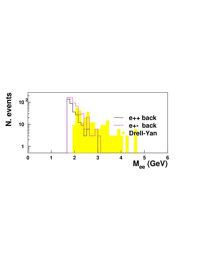
Figure 28: Background estimation for the collider mode. The Drell–Yan signal is generated with a minimum invariant mass of $2$ $\rm GeV/c^{2}$. The background below $1.5$ $\rm GeV/c^{2}$ is not shown since it is vetoed by the trigger. Only the gamma conversions taking place before the second tracking layer are taken into account. A perfect performance of the PID and tracking system is supposed here. The generated statistics is $4\cdot 10^{9}$ $\overline{p}p$ interactions, corresponding to about 4 hours of data taking at a luminosity of $5\cdot 10^{30}$ $\rm cm^{-2}s^{-1}$.

For the count rate estimates, we will focus on the Drell–Yan process, the reaction with the highest demand on luminosity. Other reaction channels of interest have larger cross–sections or, like single–spin asymmetries, may use an unpolarized antiproton beam.

The experimental uncertainty for double–spin asymmetries depends on the number of observed events $N$ as well as on the degree of polarization of the two beams. A value of ($P~{}\mathrel{\hbox to0.0pt{\lower 4.0pt\hbox{\hskip 1.0pt$\sim$}\hss}\raise 1.0pt\hbox{$>$}}~{}0.80$) can be assumed for the proton beam polarization, whereas values of $Q~{}\approx~{}0.30$ are anticipated for the antiproton beam polarization [123], see Sec. 8. The error is then roughly given by $(PQ\sqrt{N})^{-1}=4/\sqrt{N}$. It should be noted that an extensive study is foreseen to optimize the spin–filtering process: any beam polarization acquired in addition by the antiproton beam will reduce experimental uncertainties linearly.

Figure 29: Expected precision of the $h_{1}$ measurement for one year of data taking at 50 % efficiency (180 days). An indicative $A_{TT}/\hat{a}_{TT}=0.3$ has been considered in the simulation. For the collider mode a luminosity of $5\cdot 10^{30}$ $\rm cm^{-2}s^{-1}$ and a polar angle acceptance between $20^{\circ}$ and $130^{\circ}$ was assumed (left). For the fixed–target mode at 22 GeV/c beam momentum a luminosity of $2.7\cdot 10^{31}$ $\rm cm^{-2}s^{-1}$ and a polar angle acceptance between $5^{\circ}$ and $50^{\circ}$ was assumed (right).

For every event, the Bjorken $x$ of the proton and $\overline{x}$ of the antiproton can be extracted from the measured invariant mass ($M^{2}=Q^{2}$) and from the longitudinal momentum ($p_{L}=s/2\cdot x_{F}$) of the lepton pair. In the $u$ dominance hypothesis the $A_{TT}(x,\overline{x})$ asymmetry is related to the convolution of the transversity distributions $h_{1}(x)\cdot h_{1}(\overline{x})$ by the relation

$$A_{TT}(x,\overline{x})=\hat{a}_{TT}\;\frac{h_{1}(x)}{u(x)}\frac{h_{1}(\overline{x})}{u(\overline{x})}\;.$$

During one year of data taking, $h_{1}(x)$ can be measured in a wide $x$ range, from $0.7$ down to $0.05$, covering the most interesting valence region and extending to low values of $x$ where theoretical predictions show the largest deviations. The precision achievable in 180 days (one year of data taking with 50 % of efficiency) is shown in Fig. 29. These numbers entail only the non–resonant contribution to the Drell–Yan process: the $J/\Psi$ will enhance the number of events in the $M^{2}$ = 6–16 GeV² range considerably.

For low–$t$ proton–antiproton elastic scattering, recoil–detectors, with a typical area of 5$\times$4 cm² each, will be mounted with an angular acceptance matched to the center of the storage cell. Count rates of 6$\times 10^{6}$/week per $t$–bin of 0.0005 GeV² width are expected to be achieved with a polarized antiproton beam of $P=30\%$ polarization. Assuming a target polarization of $Q=90\%$ spin correlation parameters can be measured to a precision of 0.01 within a week, so this program can be finished within a few weeks of beam time.

19 Alternative Scenarios

Two alternative scenarios were considered for the detector design. The first is to select Drell–Yan events with muons. The second is to use a conventional solenoid magnet as spectrometer magnet for the collider mode.

19.1 Drell–Yan with Muons

The design of a detector for Drell–Yan with muons at the PAX energies presents a host of difficulties, which make this a challenging task. The only known way of separating muons from hadrons is to use their low interaction probability and consequent high capability of penetrating large amounts of heavy absorbing material. The hadronic background can originate from decays of charged pions and kaons before reaching the absorber and from hadrons penetrating the material (punch–through). At PAX energies, a typical detector with about 1 m of space before the absorber for charged particle tracking, particle identification and electron/photon detection, cannot guarantee a $\pi/\mu$ rejection factor of $10^{2}$ [190] due to the high probability of meson decays. These decays could be only reduced by moving the absorber closer to the interaction region at the expense of completely losing all the flexibility of the experimental facility. In any case, empty space has to be foreseen for the vacuum chamber as a housing for the vertex detector, so that the secondary–muon rejection factor can hardly exceed $10^{3}$. The absorber puts also severe limitations on the achievable resolution of the dilepton invariant mass. This approach was extensively adopted in the past for Drell–Yan measurements, but at a much higher energy where the decay probability reduces and the absorber filtering is more effective. To keep the background at an acceptable level and not being able to isolate the charmed resonances from the continuum due to the poor resolution, those experiments are limited to a kinematic range of dilepton invariant masses larger than 4 GeV [191]. Such a constraint would limit both the achievable statistics and the covered range in Bjorken $x$ at PAX. Even a large number of heavily instrumented material segments do not suppress hadrons faking muons entirely. Refined studies at the B–meson $e^{+}e^{-}$ facilities show that the maximum rejection factors against hadron punch–through achievable with active absorbers are of the order of $10^{3}$ [192, 102]. The above values of pion rejection factors are well below the $10^{4}$ to $10^{5}$ threshold required for an efficient Drell–Yan measurement.

Since there are several powerful well–established techniques to distinguish electrons from pions in the energy range of the PAX experiment, and since these are compatible with a precise measurement of the particle momenta, the Drell–Yan electron channel was selected to be a much more effective solution for PAX.

19.2 Solenoid Magnet

A solenoid field is a natural option for a collider detector since it provides an almost homogeneous field in a large empty volume suitable for tracking. This choice presents some drawbacks for the PAX physics case. Since the spin of the beam particles undergoes precession inside the longitudinal field of the spectrometer, a set of counteracting–solenoids inside the interaction region is required such that the longitudinal field integral that protons and antiprotons experience before a collision vanishes. Although it is in principle feasible, this solution would complicate the design of the collider IP. The correction has to work for any beam momentum employed in order to vary the center–of–mass energy of the collisions and explore different kinematic regimes. Moreover, the correction can not be exact over the about 30 cm long IP bunch–length and the unavoidable spin precession will be energy dependent. The solenoid is not compatible with a transverse polarized target, hence is not suitable for Phase–I or Phase–II (b) of the PAX physics program (see Sec. 13 and 14).

Because the threshold Čerenkov detector can not be efficiently operated in the strong field of a solenoid magnet, a possible alternative is to employ a transition radiation detector (TRD). The transition radiation, being proportional to the relativistic $\gamma$ factor of the particle, is effective at high momenta and the required $10^{3}$ pion rejection factor might represent a challenge at PAX energies [193, 194]. Additionally, TRDs typically add ten times more material than a Čerenkov detector (more than 0.1 radiation length), thus enhancing gamma conversions and energy losses by radiation of the Drell–Yan electrons. Triggering on rare di–electron events in the high–multiplicity PAX environment is not trivial. A pattern recognition, required to link the electromagnetic signatures to the helicoidal trajectory of the particle, is possible only with massive use of computing power.

It is desirable to match the bending power of the spectrometer to the momenta of the emerging particles. In the forward region, where the angle between the particle path and the beam direction is small, the rigidity increases and it is more difficult to provide the necessary bending power. A solenoid centered on the beam provides the maximum bending at large angles in the laboratory frame. Since there is no transverse force on a particle traveling along a magnet field line and the solenoid field lines are parallel to the beam axis, bending is reduced eventually to zero, as the scattering angle is decreased to zero.

The torus has none of the above drawbacks. It neither disturbs the beams nor the operation of the Čerenkov detector since the generated field is limited to a well defined region with negligible fringe fields. The field lines of a toroid field centered on the beam line are always perpendicular to the paths of particles originating from the axis. Its field intensity increases inversely with radius from the beam, such that larger bending power becomes available at small angles. The drawbacks of the toroid could be a not homogeneous field and the presence of the coil material inside the tracking volume. The first issue simply requires to use a detailed field map for tracking. As a conservative approach, it is planned to exploit the over–constraint kinematics of the physical channels of PAX during Phase–I to test and optimize the spectrometer performance before starting the more challenging measurements of PAX Phase–II. The second issue causes a reduction of the azimuthal acceptance; the loss in acceptance can be minimized by using superconducting technology to save material and by placing the support structures and utility lines of the detector in the blind region of the toroid coils. The approach of PHENIX to use Helmholtz coils together with large field–driving magnet yokes would have an even more severe impact on the azimuthal acceptance [195]. Due to the arguments mentioned above a toroidal field approach has been taken to be more suitable for the PAX program than a solenoid field. A feasibility study about the possibility to use the PANDA detector in the collider–mode must necessarily be started on the basis of the arguments discussed above.

Part V Organization

20 Logistics of the Experiment

20.1 Floor Space

As mentioned in chapter 7, all rings of the HESR complex should be in one plane. It is assumed that a hall for the CSR is provided, similar in space as the COSY hall. The APR is located inside the CSR. Furthermore we assume that PAX is the only user of CSR, allowing for a permanent installation of the PAX detector in one of the straight sections. For the experiment, a total space of about 300 m² is required. If the experiment has to be moved in and out, this space has to be enlarged to about 450 m².

Concerning the required height of the experimental hall, we assume a beam 3 m above the platform and 5 m above the floor. The upper edge of the detector frames is assumed at 7.5 m above floor, resulting in a maximum height of the crane hook of 10.5 m above the floor. With 1.5 m for the crane structure itself, an inner hall volume for the fixed experiment of about 3600 m³ and for the movable experiment of about 5400 m³ is estimated (Tab. 10).

Height of the experimental hall	12 m
Crane hook	10.5 m above floor
Assumed beam height	5 m above floor
Volume of the hall (exp. fixed)	300 m${}^{2}\times 12\,{\rm m}=3600$ m3
Volume of the hall (exp. movable)	450 m${}^{2}\times 12\,{\rm m}=5400$ m3

Table 10: Requirements of the experimental hall for PAX.

In addition laboratory space and a control room attached to the experimental hall are required.

20.2 Radiation Environment

The PAX experiment will operate with long beam lifetimes and thus slow antiproton consumption. Requirements for radiation safety at the target location will not be enhanced with respect to other areas along the HESR.

20.3 Responsibilities and Manpower

Although the APR needs institutional responsibilities, we assume that after demonstration and testing the APR will become part of the FAIR facility and is operated and maintained by the laboratory, i.e. GSI.

20.3.1 Institutional Responsibilities (preliminary list)

• Antiproton Polarizer Ring
  Ferrara, Jülich

• Targets (APR, CSR/HESR)
  Ferrara, Erlangen, Jülich, Gatchina, Madison

  • Target Magnet
    Ferrara, Gatchina

• Large–Acceptance Spectrometer

  • Toroid Magnet
    Ansaldo (Italy)

  • Vertex Detector
    Jülich

  • Electromagnetic Calorimeter
    Frascati, Moscow, Protvino, and Yerevan

  • Drift Chambers
    Gatchina, Dubna

  • Threshold Cherenkov
    Dubna, Gent

• Forward Spectrometer (optional)

  Partially recuperated from the HERMES experiment.

  • Particle Identification
    Dubna

• Data Acquisition and Trigger
  Dubna, Protvino, Gatchina, Jülich

• Computing, Technical Software, Simulations
  Ferrara, Tbilisi, Dubna, Beijing, Hefei

20.3.2 Manpower

The present status of manpower available for the experiment can be inferred from the Collaboration list (see p. 5ff). The list comprises about 170 participants from 13 countries and 35 institutions. Based on inquiries and discussions, we expect a very significant further growth of the collaboration in the next couple of years.

20.4 Schedule

20.4.1 Milestones

#	Date	Milestone
1	12/2006	Technical Design Reports finished; overall design of all PAX components
2	12/2008	Fabrication of APR components finished
3	12/2010	Spin filtering with protons in the APR tested
4	12/2010	Fabrication of detector components finished
5	12/2011	CSR operational with protons at FAIR
6	12/2012	Installation of PAX detector (Phase–I) finished
7	12/2013	Commissioning of PAX detector (Phase–I) with protons/antiprotons done
8	12/2013	Phase–I polarized antiproton facility (CSR & APR) ready for experiments
9	$>$ 2015	Commissioning of HESR in the (Phase–II) double–polarized collider mode

Table 11: Milestones of the PAX experiment.

20.4.2 Timelines

The timelines of the PAX experiment depend on the FAIR schedule, the availability of recuperated equipment, like components of the HERMES experiment, and on manpower and funding. A first scenario is presented in Fig. 30. It is based on the assumption that the Phase–I polarized antiproton facility is available in 2013, ready to accept antiprotons from the new antiproton source.

A central part of PAX is the antiproton polarizer ring (APR) which is required to be operational in 2010 for proton tests. Because of the availability of a polarized proton injector at Jülich, we prefer to set up the APR at COSY for proton tests as soon as possible. Installation and running–in at FAIR is scheduled for 2011/12. Furthermore, we assume that the CSR is fully operational at FAIR in 2011, and that the full CSR antiproton facility including the Phase–I PAX detector is available for proton tests in 2012, including acceleration of polarized beams.

The PAX detector is located permanently in the CSR straight section. It consists of the Large–Angle Spectrometer (LAS) and an optional Forward Spectrometer (FS). The FS is largely based on components recuperated from the HERMES detector. Commissioning of the full Phase–I detector is scheduled for 2013.

Two polarized internal gas targets (PIT) exist which can be utilized after improvements and modifications. PIT–I is the present HERMES target which is available in 2006, after the double–spin program is terminated. This target has been in operation since 1996. After a suitable upgrade, it can be installed at the APR in 2009 for proton tests. In addition, a development program at INFN Ferrara is conducted in order to study possible improvements by using superconductive sextupole magnets for a higher source intensity. PIT–II is the present ANKE target which will be available only after 2009 or later. It is foreseen for installation into the PAX detector at CSR.

Figure 30: Time Schedule for the PAX experiment.

20.5 Cost Estimates

The cost estimate for the fixed energy APR, listed in Table 12, is based on a ring built from permanent magnet material, which is a very economic solution, since there are no power supplies needed. For the same reason, the cost of operation is substantially reduced compared to a ring built from electromagnets.

The cost estimate for the PAX detector is divided into four main categories, which are briefly discussed below. The resulting figures, listed in Tab. 13, are based on the 1993 figures of the HERMES TDR [184], and were increased by 30% for inflation.

1. Large–Acceptance Spectrometer: Here the structure of the E835 detector has been assumed with the addition of a toroidal spectrometer magnet, calculated using HERMES figures (Cherenkov and Calorimeter), and the price of the HERMES recoil detector for the tracking part.

2. Forward Spectrometer: Here the cost is extrapolated from the one estimated for the Large–Acceptance Spectrometer, with the additional cost for hadron identification (from HERMES RICH).

3. The polarized target is needed for the fixed–target mode only. Here parts of the HERMES and/or ANKE targets can be recuperated, which should result in a reduction of the order of 40%.

4. Infrastructure: These costs are also based on HERMES figures for platform and support structures, cabling, cooling water lines, gas supply lines and a gas house, cold gases supply lines, electronic trailer with air conditioning etc.

Polarized target (HERMES)	1.0 MEU
Machine (permanent magnet version & vacuum)	6.0 MEU
Electron cooler	1.5 MEU
Injection/beam lines	0.5 MEU
Snake	0.2 MEU
Polarimeter	0.2 MEU
Total	9.4 MEU

Table 12: Cost estimate for the Antiproton Polarizer Ring (APR)

Toroid magnet	3.0 MEU
Polarized target (required only for fixed–target mode)	1.0 MEU
Large–Acceptance Spectrometer (LAS)	12.0 MEU
Forward Spectrometer (FS) (optional)	(5.0) MEU
Infrastructure (cabling, cooling, shielding)	3.0 MEU
Total, without (with) FS	19.0 (24.0) MEU

Table 13: Cost estimate for the PAX detector.

Part VI Appendix A

Appendix A Polarization Transfer Technique & Applications

This mini–review addresses the polarization–transfer technique and its high–energy applications.

A.1 Breit Hamiltonian and Antiproton Polarizer

The spin-filtering by electromagnetic antiproton-electron interaction is at the core of the proposed PAX experiment and a brief review on the QED foundations of this technique is in order. In the spin–filtering method one depends on the $e\bar{p}$ interaction at nonrelativistic kinetic energy of electrons in the proton rest frame

$$T_{e}={m_{e}\over m_{p}+m_{e}}T_{\bar{p}}\,,$$

where $T_{\bar{p}}$ is the kinetic energy of antiprotons in the Antiproton Polarizer Ring (APR). This interaction is described by the celebrated Breit Hamiltonian. In its application to the electron–proton interaction, ever since its derivation 75 years ago, in 1929, [1], the Breit Hamiltonian (improved for the anomalous magnetic moment of nucleons) has been the fundamental tool of atomic physics. It is found in any textbook on QED and atomic physics [2, 3] and need not be reproduced here. From the point of view of spin–dependence, it contains the spin–orbit, spin–tensor and hyperfine spin–spin interactions.

Now, recall that in the scattering of spin–0 particles off spin–${1\over 2}$ particles the target–spin asymmetry (analyzing power) and normal polarization of the recoil spin–${1\over 2}$ particle equal each other: $P_{y}=A_{y}$. In the more complex case of

$${1\over 2}+{1\over 2}\to{1\over 2}+{1\over 2}$$

scattering, the number of polarization observables is much higher [4]. Evidently, the existence of spin–tensor and hyperfine interactions would give rise to a beam–target double–spin asymmetry. Simultaneously, they entail the correlation between induced polarizations of scattered particles and, most importantly for the present discussion, of the polarization transfer from the polarized beam particle to the recoil target particle. For the Breit interaction the relationships between these observables are trivial; the general discussion with application to nucleon–nucleon interactions is found in the classic review by Bystricky et al. [4].

The Horowitz–Meyer derivation [5] of the polarization transfer from electrons in the polarized hydrogen atom to scattered (anti)protons can be described as based on the Breit Hamiltonian, although they use directly the relativistic approach and skip Breit’s reduction to the non–relativistic formalism. In terms of the Breit Hamiltonian, the factor of 2 difference between the transfer of the transverse and longitudinal polarizations from the electron to proton stems from the spin–tensor interaction.

A.2 Polarized Electron–Proton Elastic Scattering: Theory

Now we turn to a brief overview of applications to high–energy electron–nucleon scattering and the independent determination of the charge and magnetic moment structure of nucleons. Our coverage is far from being complete as we only wanted to emphasize an enormous advance in the form factor studies resulting from the electron–to–nucleon polarization transfer technique.

In 1957 Akhiezer et al. published the first analysis of the scattering of polarized electrons on polarized protons [6]. They noticed correctly that polarization effects could in principle be applied to determine $G_{E}$. In the quest for methods to determine the longitudinal polarization of leptons produced in weak interactions, Bincer in 1957 considered the electromagnetic scattering of longitudinally polarized leptons on leptons [7]. Electron–proton scattering for arbitrary polarizations, with allowance for the anomalous magnetic moments, has been treated by Scofield in 1959 ([8], see also the follow–up paper on three and four spin observables [9]).

The modern treatment of the scattering of polarized leptons at high energy is for the most part based on the 1969 Rev. Mod. Phys.  paper by N. Dombey [10]. For ultrarelativistic electrons the dependence on the transverse polarization of the electron vanishes. This is a consequence of the conservation of the helicity of ultrarelativistic electrons in high–energy QED, first noticed in 1954 by Yennie, Ravenhall and Wilson ([12], see also the textbook [13]). This is precisely the phenomenon by which the transverse polarization effects can only be seen in the annihilation processes $e^{-\uparrow}\vec{e}^{+\uparrow}\to\mu^{+}\mu^{-},q\bar{q}$, or in the Drell–Yan reaction $q^{\uparrow}\bar{q}^{\uparrow}\to e^{+}e^{-}$. Dombey shows that when the incident lepton is longitudinally polarized, the virtual photon is in a pure polarization state which is a coherent superposition of an elliptically polarized transverse state and a longitudinal state.

Extracting the new information contained in the interference between $xy$, i.e., $TT^{\prime}$, and $yz$, i.e., $LT$ components of the photon absorption amplitude, requires scattering off polarized targets or, alternatively, measurements of the recoil polarization. Dombey made a strong point, implicitly contained in Ref. [6] and especially in the 1968 paper by Akhiezer and Rekalo [11], that the most interesting experiment is to measure an interference term of the form $G_{E}G_{M}$ and so find $G_{E}$, including its sign. Dombey emphasized that the possibility of $G_{E}$ changing its sign at large $Q^{2}$ is not excluded. The target must be polarized perpendicular to the virtual photon in the Breit frame, i.e. perpendicular to the direction of the recoil nucleon in the laboratory and in the scattering plane. In modern language, one must measure the double–spin longitudinal–transverse asymmetry. The double–spin longitudinal–longitudinal asymmetry is proportional to $G_{M}^{2}$ (see also Eq. (1) below). Both the double–spin asymmetry and electron–to–proton polarization transfer techniques have been applied subsequently at SLAC, MIT–Bates, MAMI and Jlab.

A.3 Beam–target Double–spin Asymmetry and $G_{E}/G_{M}$

The first determination of the sign of $G_{E}/G_{M}$ by the double–polarization asymmetry in $\vec{e}\vec{p}$ elastic scattering at $Q^{2}=0.765$ GeV² was performed in 1976 at SLAC [14]. The authors comment that the practical usefulness of the method at higher $Q^{2}$ is limited by low counting rates. The first double polarization measurements of the neutron electric form factor via neutron knockout from a polarized ³He target, ${}^{3}\vec{\mathrm{He}}(\vec{e},e^{\prime}n)$, were carried out by the MAMI collaboration ([15], for the subsequent MAMI experiments see [16, 17] and references therein). In several Jlab experiments the neutron form factor has been evaluated from quasielastic scattering off polarized deuterons, $\vec{d}(\vec{e},e^{\prime}n)$ [18, 19, 20]. An excellent summary of these data is shown below in Fig. 31, borrowed from the MAMI publication by Glazier et al. [17].

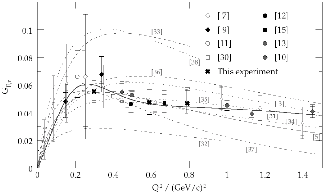
Figure 31: $G_{E,n}$ from double–polarization experiments as compiled by Glazier et al. (MAMI) [17]. Polarization–transfer measurements on the deuteron [38, 40, 39] are marked with diamonds, experiments using polarized Deuterium [18, 19, 20] or ${}^{3}\vec{\rm He}$ [43, 36] targets are shown as circles and squares, respectively. ”This experiment” refers to the MAMI experiment by Glazier et al. [17]. Open triangles refer to the analysis [42] of unpolarized data. The thin full curve represents the original Galster parameterization [41], the thick line represents the “pion–cloud” parameterization [44] (see text). The legend of the dashed and dotted lines is found in Ref. [17].

A.4 Electron Proton Polarization Transfer and $G_{E}$/$G_{M}$: Theory

The advantages of the electron–to–proton and electron–to–neutron polarization transfer technique were recognized in 1974 by Akhiezer and Rekalo [21] and elaborated in 1981 by Arnold, Carlsson and Gross [22]. The method requires that the polarization of the recoiling nucleon be measured in a second, analyzing, scattering. The recoil nucleon is polarized in the scattering plane and has polarization components either transverse (sideways), $P_{T}$, or longitudinal, $P_{L}$, to its momentum:

$$P_{T} = hD_{LT}={h\over I_{0}}\cdot\left(-2\sqrt{\tau(1+\tau)}G_{M}G_{E}\tan{\theta_{e}\over 2}\right)$$

$$P_{L} = hD_{LL}={h\over I_{0}}\cdot{E+E^{\prime}\over M_{p}}\cdot\sqrt{\tau(1+\tau)}(G_{M})^{2}\tan^{2}{\theta_{e}\over 2}\,.$$ (44)

Here $h$ is the helicity of the incident electron, $E$ and $E^{\prime}$ are the laboratory energies of the incident and scattered electron, respectively, $\theta_{e}$ is the electron scattering angle and $I_{0}$ is the unpolarized cross section (excluding the Mott cross section). In accordance with general theorems [4], there is a one–to–one correspondence between the double–spin beam–target asymmetries and electron–to–nucleon polarization–transfer. The recoil polarimeters give access to the transverse polarization of the recoil particle; using spin rotation in the special spin–rotator and/or spectrometer magnets, one can measure simultaneously both $P_{T}$ and $P_{L}$ in the same polarimeter. Then the ratio of the two polarization components would give the ratio of form factors,

$${G_{E}\over G_{M}}=-{P_{T}\over P_{L}}\cdot{E+E^{\prime}\over 2M_{p}}\cdot\tan{\theta_{e}\over 2}\,.$$ (45)

Neither the beam polarization nor the analyzing power needs to be known. Because the two polarization observables are measured simultaneously, this technique avoids a major systematic uncertainty of the Rosenbluth separation. An important virtue of the polarization–transfer technique is that it is viable at large $Q^{2}$.

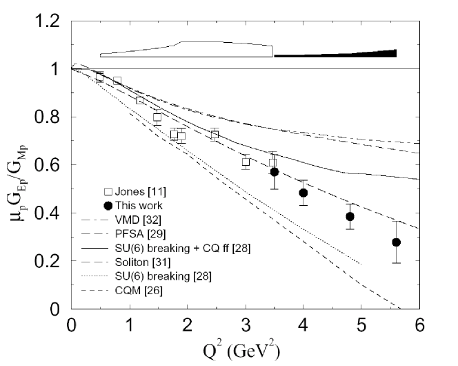
Figure 32: A compilation of the experimental data on the ratio $\mu_{p}G_{Ep}/G_{Mp}$ from the Jefferson lab experiments [25, 26] compared with theoretical calculations (for the references see [26]). Systematic errors are shown as a band at the top of the figure.

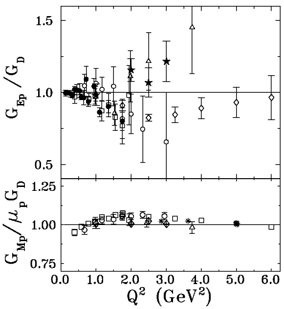
Figure 33: World data prior to 1998 for the ratio of form factors to the dipole parameterization $G_{D}$: (a) $G_{E}^{p}/G_{D}$ and (b) $G_{M}^{p}/\mu_{p}G_{D}$ versus $Q^{2}$. Refs. Litt et al. ($\triangle$) [28], Berger et al. ($\Box$) [29], Price et al. ($\bullet$) [30], Bartel et al. ($\circ$) [31], Walker et al. ($\star$) [32], Andivahis et al. ($\Diamond$) [33] and Sill et al. ($\ast$) [34].

A.5 Electron Proton Polarization Transfer: Experiment

Milbrath et al. were the first to apply recoil polarimetry to the determination of $G_{E}/G_{M}$ at low $Q^{2}$ for protons in the MIT–Bates experiment [23]. Similar measurements have been carried out at MAMI [24]. Particularly noteworthy is a series of beautiful large–$Q^{2}$ experiments at Jlab [25, 26] which resulted in the discovery of a steep decrease of the ratio $G_{E}^{p}/G_{M}^{p}$ with $Q^{2}$ which continues to the largest $Q^{2}$ studied (see Fig. 32, borrowed from Ref. [26]). These results must be compared to the world data prior to 1998 shown in Fig. 33, borrowed from Punjabi et al. [27]. The latter paper gives an excellent introduction to the experimental realization of the polarization–transfer technique.

The polarization–transfer technique has led to a dramatic improvement in the determination of $G_{E}^{p}/G_{M}^{p}$, which inspired the recent flurry of theoretical interest in the time–like form factors discussed in Section 4 of the PAX Technical Proposal. A very detailed discussion of implications of the new data for the theoretical description of form factors is found in Ref. [27].

A.6 Electron–to–Neutron Polarization Transfer and $G_{E}^{n}/G_{M}^{n}$: Experiment

The polarization–transfer technique proved equally fruitful in applications to the quasielastic scattering off polarized deuterons and as a source of information on the neutron form factors. Arenhövel et al. made an important point [35] that in the application of the technique to quasifree scattering off the deuteron, the corrections for final state interactions, meson exchange currents, isobar configurations, and the models of the deuteron structure, are well under control (for a further theoretical analysis of quasifree scattering off ${}^{3}\mathrm{He}$ within the Faddeev approach and the comparison of extraction of $G_{E}^{n}$ from quasifree scattering off the ${}^{3}\mathrm{He}$ and deuterium targets see [36]). This point has been confirmed experimentally by a direct comparison of the determinations of $G_{E}^{p}/G_{M}^{p}$ from recoil polarimetry in elastic, $\vec{e}p\to\vec{p}e$, and quasielastic, $\vec{e}(d,\vec{p}e^{\prime})$, scattering. The MIT–Bates experiment by Milbrath et al. [23] was the first to do so at low $Q^{2}$, and the results from the large–$Q^{2}$ Jlab experiment are reported in Ref. [37], where one would find further references.

Eden et al. in 1994 were the first to apply the polarization–transfer technique at MIT–Bates [38]; subsequently it has been used at MAMI [17] and Jlab ([39] and references therein). Madey et al. [39] make a convincing point that the recoil polarimetry made facilitated measurements at $Q^{2}$ as large as 1.13, and 1.45 (GeV/c)², which had never been achieved before in polarization measurements. Figure 31, borrowed from Ref. [17], summarizes the experimental data on $G_{E}^{n}$ from double–polarization experiments.

Besides the much smaller error bars compared to those provided by analysis of the earlier data from unpolarized scattering, the interpretation of the recoil–polarimetry data is free of model uncertainties inherent in the interpretation of the unpolarized data. This particular point prompted the use of polarization transfer in ${}^{4}\mathrm{He}(\vec{e},e^{\prime}\vec{p})^{3}\mathrm{H}$ by a recent Jlab experiment [45] as a sensitive probe of the long sought modification of the form factors of a proton bound in a nucleus ([45] and references therein).

A.7 Summary

The electron-to-proton polarization transfer at energies of the Antiproton Polarizer Ring (APR) is a simple quantum-mechanical problem based on the Breit Hamiltonian which has been derived in 1929 from fundamental QED. Ever since its derivation the Breit Hamiltonian has been at the core of the atomic physics. At relativistic energies precisely the same QED mechanism describes double-spin asymmetries in the scattering of longitudinally polarized electrons on polarized nucleons and/or the polarization transfer from longitudinally polarized electrons to recoil nucleons. In high-energy experiments the interest is not in testing the straightforward QED calculations per se, rather the polarization-transfer, in conjunction with the recoil polarimetry, has become a fundamental tool for the high-precision determinations of the charge and magnetic moment distributions in protons and neutrons. The unprecedented accuracy achieved in those experiments uncovered the properties of the form factors which triggered a lively theoretical dispute on the onset of hard pQCD asymptotics both in the space like and time like region, which is behind the experimental program outlined in this document.

Part VII Appendix B

Appendix B Polarized Antiproton-Proton Soft Scattering

In this Appendix we comment in more detail on the impact of the spin-dependence of antiproton-proton interaction on the interpretation of the Coulomb-Nuclear Interference data and on the special interest in double-polarized antiproton-proton scattering at very low energies in view of the indications for the protonium state.

B.1 Spin effects in the Interpretation of Coulomb–Nuclear Interference

The compilation of the experimental data on the ratio of the real to imaginary part, $\rho$, of the $p\bar{p}$ forward scattering amplitude, shown in Sec. 6.1 of the PAX Technical Proposal suggests a substantial departure of the experimental data points from the dispersion theory calculations (DT). The extraction of $\rho$ from the experimentally measured differential cross section of elastic scattering in the Coulomb-Nuclear Interference (CNI) region is usually done assuming a negligible spin dependence of the elastic scattering amplitude:

$${d\sigma\over dt} = {\pi\over p^{2}}\bigl{|}f_{C}\exp(i\delta_{B})+f_{N}\bigr{|}^{2}={d\sigma_{C}\over dt}+{d\sigma_{int}\over dt}+{d\sigma_{N}\over dt}\,,$$ (46)

$${d\sigma_{C}\over dt} = {4\pi\alpha_{em}^{2}G_{E}^{4}(t)\over\beta^{2}t^{2}}\,,$$ (47)

$${d\sigma_{N}\over dt} = {\sigma_{tot}^{2}(1+\rho^{2})\over 16\pi}\cdot\exp(-B|t|),$$ (48)

$${d\sigma_{int}\over dt} = {\alpha_{em}^{2}\sigma_{tot}G_{E}^{2}(t)\over\beta|t|}\cdot(\rho\cos\delta_{B}+\sin\delta_{B})\cdot\exp(-{1\over 2}B|t|)\,.$$ (49)

Jakob and Kroll [1] make a point that

• The optical point at $t=0$,

  $${d\sigma\over dt}\bigr{|}_{t=0}={1\over 16\pi}\left({1\over 4}\sigma_{s}^{2}(1+\rho_{s}^{2})+{3\over 4}\sigma_{t}^{2}(1+\rho_{t}^{2})\right)$$ (50)

  will differ from given by formula (3) with the spin averaged quantities,

  $$\sigma_{tot} = {1\over 4}\sigma_{s}+{3\over 4}\sigma_{t}\,$$ (51)

  $$\rho = {1\over\sigma_{tot}}\left({1\over 4}\sigma_{s}\rho_{s}+{3\over 4}\sigma_{t}\rho_{t}\right)\,.$$ (52)

  where, for the sake of illustration, we only consider the simplest example with

  $$f_{N}=\left({1\over 4}f_{s}+{3\over 4}f_{t}\right)+(f_{t}-f_{s})(\vec{s}_{p}\vec{s}_{\bar{p}})\,,$$ (53)

  the discussion of the general case is found in [1].

• The $t$-dependence of amplitudes $f_{s,t}$ for the spin-singlet and spin-triplet states could be different, i.e., taking one and the same diffraction slope $B$ in the exponential $t$-dependent factors in the strong interaction term (49) and the CNI term (49) is an assumption which must be tested experimentally

• The so-called Bethe phase, $\delta_{B}$, between the Coulomb and the strong-interaction amplitudes can vary from one spin state to another.

Figure 34: Predictions for the momentum-dependence of the spin-singlet, spin-triplet and spin-averaged antiproton-proton total cross section for the two models of $p\bar{p}$ interaction described in the text.

The spin-dependence of antiproton-proton scattering is an entirely uncharted territory and in order to get an idea on the expected effects one must resort to predictions of phenomenological models. Such models were developed earlier in connection with the experimental studies of the interactions of unpolarized antiprotons at LEAR and CPLEAR. We illustrate the major points on an example of the spin-singlet and spin-triplet forward scattering amplitudes evaluated in two $N\bar{N}$ models developed by the Jülich group [2, 3] within the meson-exchange picture. Specifically, we show here predictions of the models A(BOX) and D introduced in Refs. [2] and [3], respectively. The elastic part of these $N\bar{N}$ interaction models is obtained by a G-parity transform of the full Bonn $NN$ potential [4]. In case of A(BOX) annihilation is accounted for by a phenomenological spin-, isospin- and energy-independent complex optical potential of Gaussian form. Model D utilizes the same elastic part. However, annihilation is now described in part in terms of microscopic baryon-exchange processes based on $N$, $\Delta$, $\Lambda$, $\Sigma$, and $Y^{*}$ exchange and involving $N\bar{N}{\to}$ 2 meson decay channels with all possible combinations of $\pi$, $\eta$, $\rho$, $\omega$, $a_{0}$, $f_{0}$, $a_{1}$, $f_{1}$, $a_{2}$, $f_{2}$, $K$, $K^{*}$ - see Ref. [3] for details. For both models the results for the total and the integrated elastic and charge-exchange cross sections as well as for angular dependent observables are in good agreement with the available experimental information [2, 3].

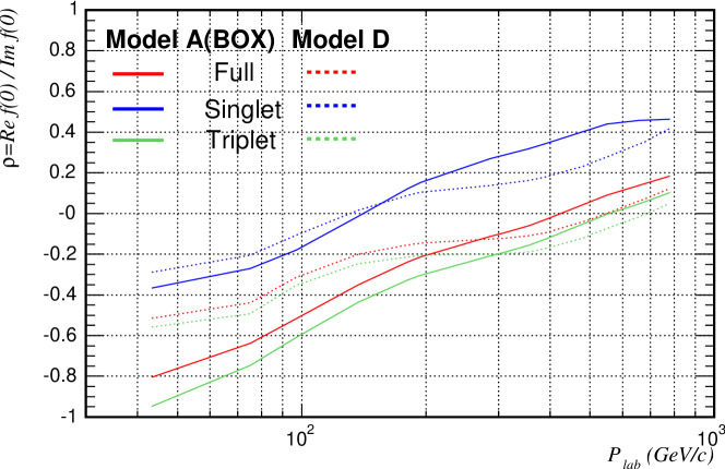
Figure 35: The momentum-dependence of the ratio of real and imaginary parts of the spin-singlet, spin-triplet and spin-averaged forward antiproton-proton scattering amplitudes as predicted by the two models for $p\bar{p}$ interaction described in the text.

In Fig. 34 we show the momentum dependence of the total cross section for the spin-triplet, spin singlet and spin-averaged interactions. Both models predict a dominance of the spin-triplet cross section over that in the spin-singlet case, typically by the factor $\sim 5$. The difference between the predictions from the two models is marginal. In Fig. 35 we show the ratio of the real to imaginary part for the amplitude of forward elastic scattering in the spin-triplet and spin-singlet states. To this end one must recall, see Figure 8 in the PAX TP, that in the considered momentum range the statistical error bars in the experimental data points for $\rho$ are of the order of $\Delta\rho\sim 0.05$. This must be contrasted with the very large variation of $\rho$, by $\approx 0.4$, from the spin-triplet to the spin-singlet state. Furthermore, the departure of predictions of the models from each other is of the order of 0.1. These results, in conjunction with the related results for the total cross section, suggest a substantial spin dependence of low and intermediate energy antiproton-proton interactions and make a strong case for the low-$t$ physics with polarized antiprotons scattering on polarized protons.

Such measurements at Phase-I will cover precisely the most interesting range of momentum, in which the early experimental data on $\rho$ exhibit a nontrivial momentum dependence and where the DT calculations and the data from the previous experiments seem to diverge most. The further measurements can also be extended to Phase-2 in the fixed target mode.

B.2 Separation of Spin–Singlet and Spin–Triplet Scattering at Low Energy

If polarized antiprotons stored in CSR can be decelerated down to $\sim 10$ MeV or still lower energies, one can also study the spin-dependence of the $N\bar{N}$ interaction at very low energies. This interaction is of strong relevance for the interpretation of the $p\bar{p}$ mass spectrum measured recently by the BES collaboration in the decay $J/\Psi\to\gamma p\bar{p}$ [5], which shows a strong enhancement near the $p\bar{p}$ threshold. The observed enhancement led to speculations that one has found a signal of an $N\bar{N}$ bound state (protonium) or an indication for a so far unobserved narrow resonance with the quantum numbers $J^{PC}$ = $0^{-+}$ or $0^{++}$ [5]. Investigations by Sibirtsev et al. [8] (among others) have shown that the interpretation of this enhancement in terms of the final state interaction in the $p\bar{p}$ system is not excluded. However, one has to keep in mind that the $p\bar{p}$ system in the $J/\Psi\to\gamma p\bar{p}$ decay is in a spin-singlet state near threshold and the corresponding $p\bar{p}$ cross section is very small compared to the spin-triplet cross section, as mentioned above, see Figure 34. As a consequence the spin-singlet amplitudes predicted by the models are only poorly constrained by the presently available $N\bar{N}$ data and, therefore, solid conclusions on the origin of the strong enhancement seen by the BES collaboration in the $p\bar{p}$ mass spectrum cannot be made at present. A measurement of the spin-dependence of $N\bar{N}$ interaction at low energies would certainly help to clarify this issue. Challenging though such a deceleration is, the cross sections one needs to measure are in the several hundred millibarn range, and the recoil detector described in Section 16.8 of the PAX TP can still be operated even at such low energies.

B.3 The Impact of the Spin–Dependence of Antiproton–Proton Scattering on the Polarization Buildup

The above presented model calculations suggest a non–vanishing proton–to–antiproton polarization transfer. The suggested approach to the polarization buildup, as outlined in Sec. 8.2 of the PAX Technical Proposal, is based on the injection into the hydrogen gas target of two hyperfine states such that the nuclear polarization of antiprotons is close to zero. The rate of polarization buildup is determined by the reliably known electron–to–proton polarization transfer. The method of the direct experimental determination of the proton–to–antiproton polarization transfer is described in Sec. 6.2 of the PAX TP. It might happen that the proton–to–antiproton polarization transfer is so strong that one can profit from the constructive interference of the electron and proton contributions, operating the polarized target at a lower density with one hyperfine state only. The current theory of spin effects in antiproton–proton interactions can not be trusted enough to serve as a basis for the decision about the polarization buildup mode employed for PAX. In Fig. 36, we give for the case longitudinal spin transfer the ratio $R=(\sigma_{e||}+\sigma_{\bar{p}p})/\sigma_{e||}$, where $\sigma_{e||}$ is the $ep$ spin transfer cross section, depicted in Fig. 10. The spin–dependent hadronic part $\sigma_{\bar{p}p}$ was taken from the two model predictions, A(Box) (red line) and D (blue), described earlier. The behavior should be taken as an indication that a sizeable improvement in the spin–dependent cross section, responsible for the polarization buildup of antiprotons, could be achieved. During spin–filtering using both electromagnetic and hadronic contributions, $\sigma_{e||}+\sigma_{\bar{p}p}$, the polarized target has to be operated by injection of a single hyperfine state into the storage cell, whereby the target density is reduced by a factor of two compared to spin–filtering with a purely electron–polarized gas target, for which two hyperfine states can be injected. Thus, in order to benefit from the constructive interference of electron and proton contributions, the value of $R$ must be larger than two.

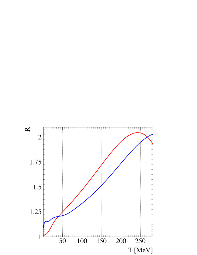
Figure 36: Energy dependence of the ratio $R=(\sigma_{e||}+\sigma_{\bar{p}p})/\sigma_{e||}$. The predictions of the two models A(Box) (red line) and D (blue) indicate a sizeable increase of the polarizing cross section in the energy range of interest.

B.4 Summary

The spin–dependence of the antiproton–proton interactions is an entirely uncharted territory. The available theoretical models were developed more than a decade ago. They give a good description of the wealth of the experimental data, predominantly on the two–body final states, from CPLEAR; however, they have never been tested against the experimental data on double–spin observables. The models indicate a fairly strong spin effects, for instance, a very strong suppression of the spin–singlet cross section.

Part VIII Appendix C

Appendix C Resonance Structures and Phase Motion of the Electromagnetic Form Factors in the Time-like Region

The experimental investigation of the time-like electromagnetic form factor of the proton has caused considerable interest in resonances in the vicinity of the proton-antiproton threshold. The $\bar{p}p\rightarrow e^{+}e^{-}$ data show considerable enhancements above the threshold, see Figure 5 in Section 4 of the PAX Technical Proposal, which can be explained by subthreshold mesons, see e.g. Refs. [5, 6, 7, 8, 9]. The point made in the PAX TP is that such structures seen in the modulus of the form factor imply, by virtue of the analyticity arguments, a nontrivial variation of the phase of form factors as a function of $q^{2}$, which can be measured in single- and double-polarized $\bar{p}p\rightarrow e^{+}e^{-}$ at Phase-I of PAX experiment. In this Appendix we discuss to more detail the impact of recent electron-positron collider results on proton-antiproton physics.

Figure 37: The $p{\bar{p}}$ scattering amplitudes for the ${}^{1}S_{0}$ and ${}^{3}S_{1}$ partial waves as a function of the center-of-mass energy. The solid lines show the results of the Jülich model while the dashed lines indicate the scattering length approximation.

C.1 Resonance Structures and Nuclear Baryonium States in $N\bar{N}$ Interactions

In the past, antiproton-proton reactions have made extremely important contributions to the knowledge about meson-like hadronic resonances. The Low-Energy Antiproton Ring LEAR at CERN has operated with low momentum antiprotons (momenta between 60 MeV/c and 140 MeV/c) in the time period between 1983 and 1996. A rich harvest of light mesons has been collected [1]. Our knowledge of scalar mesons has been substantially increased by the firm establishment of the $a_{0}(1450),f_{0}(1370)$, and $f_{0}(1500)$ and their decay modes. Two isoscalar $2^{-+}$ mesons, $\eta_{2}(1645)$ and $\eta_{2}(1870)$, and the $0^{-+}\eta(1410)$ have been observed. Moreover, an exotic $\bar{\rho}(1450)$ meson with quantum numbers $1^{-+}$ has been identified by its $\pi\eta$ decay. There is a general consensus that we have seen non-$\bar{q}q$ mesons [2].

The experimental quest for nuclear baryonia, i.e. quasibound $\bar{N}N$ states or resonances, on the other hand, never matched theoretical expectations, mainly because annihilation broadens any possible resonance structure. Some moderately broad baryonia candidates can survive, though  [4]. More details and references to early works can be found in a recent review by Klempt et al. [3].

Figure 38: Invariant $J/\Psi{\to}\gamma p{\bar{p}}$ amplitude $|A|^{2}$ as a function of the $p{\bar{p}}$ mass. The squares represent the experimental values of $|A|^{2}$ extracted from the BES data. The curves are the scattering amplitude squared ($|T|^{2}$) predicted by the $N\bar{N}$ model A(OBE) for the ${}^{1}S_{0}$ and ${}^{3}P_{0}$ partial waves and the $I{=}0$ (solid) and $I{=}1$ (dashed) channels, respectively. Note that the latter results have been normalized to $|A|^{2}$ at $M(p\bar{p}){-}2m_{p}{=}$50 MeV.

The new generation of electron-positron colliders has started to contribute to this discussion. BELLE observes threshold enhancements in B-decay, ${B^{+}}\rightarrow p\bar{p}K^{+}$ and $\bar{B^{0}}\rightarrow p\bar{p}D^{0}$, see Refs. [10, 11]. BES finds an even more pronounced threshold enhancement in the reaction $J/\psi\rightarrow p\bar{p}\gamma$, which the collaboration has interpreted as evidence for a $0^{-+}$-resonance with a mass of 1859 MeV/c², see Refs.  [12, 13]. The resonance claim has been challenged recently because a cusp effect might explain the experimental findings as well [14]. The Jülich theory group has performed calculations based on the Jülich meson-exchange potential for the $\bar{p}p$-reaction and finds that final state interactions are important but do not suffice to explain the BES data [15]. This finding leaves room for a possible resonance interpretation of the enhancement seen by BES. A recent preprint by Loiseau and Wycech is even more specific and claims that a new version of the Paris potential is compatible with a resonance in the ${}^{11}S_{0}$ partial wave [16].

C.2 $N\bar{N}$ Interaction and the Interpretation of the BES Results

The difficulties in interpreting the BES data are illustrated in the following figures. The scattering amplitudes for the ${}^{1}S_{0}$ partial wave are presented in Fig. 37. The solid lines are the result for the full amplitude while the dashed lines are based on the scattering length approximation. Note that the scattering lengths predicted by the Jülich $N\bar{N}$ model are $a_{0}{=}(-0.18{-}i1.18)$ fm and $a_{1}{=}(1.13{-}i0.61)$ fm for the isospin $I{=}0$ and $I{=}1$ channels, respectively. It is evident that the scattering length approximation does not reproduce the energy dependence of the scattering amplitude that well. For the $I{=}1$ channel the difference at an excess energy of 50 MeV amounts as much as 50 %. The difference is even more pronounced for the $I{=}0$ channel, where we already observe large deviations from the full result at rather low energies. This strong failure of the scattering length approximation is due to the much smaller scattering length predicted by the Jülich model for the $I{=}0$ partial wave.

Results for the ${}^{3}S_{1}$ partial wave are shown in the right panel of Fig. 37. Here the scattering lengths predicted by the $N\bar{N}$ model are $a_{0}{=}(1.16{-}i0.82)$ fm and $a_{1}{=}(0.75{-}i0.84)$ fm for the $I{=}0$ and $I{=}1$ channels, respectively. This partial wave cannot contribute to the reaction $J/\Psi{\to}\gamma p{\bar{p}}$.

One has to realize that the main uncertainty in estimating $p\bar{p}$ FSI effects does not come from the scattering length approximation but from our poor knowledge of the $p\bar{p}$ ${}^{1}S_{0}$ amplitudes near threshold and of the $J/\Psi{\to}\gamma p{\bar{p}}$ reaction mechanism. The scattering lengths employed in the literature are spin-averaged values. Since the ${}^{3}S_{1}$ partial wave contributes with a weighting factor 3 to the $p\bar{p}$ cross sections (and there are no experimental data on the spin-dependent observables at low energies that would allow one to disentangle the spin-dependence) it is obvious that their value should correspond predominantly to the ${}^{3}S_{1}$ amplitude. Thus, it is questionable whether it should be used for analyzing the BES data at all because the contribution of the ${}^{3}S_{1}$ partial wave to the decay $J/\Psi{\to}\gamma p{\bar{p}}$ is forbidden by charge-conjugation invariance.

Figure 39: The $p{\bar{p}}$ mass spectrum from the decay $J/\Psi{\to}\gamma p{\bar{p}}$. The circles show experimental results of the BES Collaboration [12], while the solid line is the spectrum obtained assuming a constant reaction amplitude.

The solid lines in Fig. 38 show the $p{\bar{p}}$ invariant scattering amplitudes squared for the ${}^{1}S_{0}$ and ${}^{3}P_{0}$ partial waves and the $I{=}0$ and $I{=}1$ channels. We consider the isospin channels separately because the actual isospin mixture in the final $p{\bar{p}}$ system depends on the reaction mechanism and is not known. The reaction $J/\Psi{\to}\gamma p{\bar{p}}$ can in principle have any isospin combination in the final $p\bar{p}$ state. Note that all squared $p\bar{p}$ scattering amplitudes $|T|^{2}$ were normalized to the BES data at the invariant mass $M(p{\bar{p}}){-}2m_{p}$=50 MeV by multiplying them with a suitable constant. The results indicate that the mass dependence of the BES data can indeed be described with FSI effects induced by the ${}^{1}S_{0}$ scattering amplitude in the $I{=}1$ isospin channel. The $I{=}0$ channel leads to a stronger energy dependence which is not in agreement with the BES data. We can also exclude dominant FSI effects from the ${}^{3}P_{0}$ partial waves. Here the different threshold behavior due to the $P$-wave nature cannot be brought in line with the data points very close to threshold.

One should note that the BES-data show a resonance structure in the $\bar{p}p$-invariant mass spectrum near 3 GeV/c² which corresponds to the $\eta_{c}$ meson, see Fig. 39. Another broad enhancement is seen near 2.3 GeV which might correspond to the $f_{0}(2200)$ meson.

C.3 Summary: Baryonium and $N\bar{N}$ Resonances in $p\bar{p}\to e^{+}e^{-}$

In the $p\bar{p}\to e^{+}e^{-}$ reaction the annihilation proceeds from the $S$-wave and $D$-wave spin-triplet, $J=1$ states. The charge and magnetic form factors receive different contributions from the $S$- and $D$-annihilation [17]. The above discussed BES data, in conjunction with the already available experimental evidence for the near-threshold structure in the time-like form factor, suggest that similar resonance behavior is quite likely also in the spin-triplet $S$- and $D$-waves. The phase motion of partial waves is a well known indicator for resonances; in the case of $p\bar{p}\to e^{+}e^{-}$ this phase motion is directly related to the relative phase of the time-like charge and magnetic form factors. The latter is measurable via the single- and double-spin asymmetries as discussed in Section 4 of the PAX TP. The Phase-I PAX experiment can explore the broad kinematical range from near-threshold to moderately high values of $q^{2}$ and is ideally suited to look for the phase variations associated with the expected resonance structures.

Part IX Appendix D

Appendix D Comments on Drell-Yan Cross Sections and Spin Asymmetries in the PAX Kinematic Regime

The Drell-Yan (DY) event rates and spin asymmetries reported in Section 2 of the PAX Technical Proposal are based on the leading-order (LO) formulas for the Drell-Yan cross section. The kinematical range of DY masses $M$ and of the principal scaling variable $\tau=M^{2}/s$ accessible in the asymmetrical collider mode at Phase-II are typical of the high-energy regime studied in the previous high-energy fixed-target experiments. Specifically, the masses $M$ above the $J/\Psi,\Psi^{\prime}$ resonances will readily be accessible. Here the situation with the higher order pQCD corrections to the LO formalism, as described in terms of the so-called $K$-factors, is well established. On the other hand, in the fixed-target mode at Phase-II, with Drell-Yan masses $M$ of $2-5$ GeV and relatively low center-of-mass energies of $\sqrt{s}\approx 5.5-6.7$ GeV, one is not in the “classic” regime discussed so far. A detailed theoretical understanding of Drell-Yan physics in this regime is crucial, as the interpretation of the experimentally observed $A_{TT}$ in terms of transversity relies exactly on the applicability of parton model ideas and factorization relations. Here we comment briefly on the origin of the $K$-factors and on ongoing work on the assessment of higher orders in perturbation theory as well as of non-perturbative corrections to the cross sections and spin asymmetries in this new kinematical domain.

D.1 Factorization and Perturbation Theory for the Drell-Yan Process

At high energies and large dimuon invariant mass $M$ the Drell-Yan cross section factorizes into convolutions of parton densities and perturbative partonic hard-scattering cross sections. Schematically,

$$M^{4}\,\frac{d\sigma}{dM^{2}}=\sum_{a,b}\,f_{a}\otimes f_{b}\otimes\frac{M^{4}d\hat{\sigma}_{ab}}{dM^{2}}\;+\;{\cal O}\left(\frac{\lambda}{M}\right)^{p}\;.$$ (54)

For brevity, we have considered here the unpolarized cross section, and we have also integrated over the rapidity of the lepton pair. The partonic cross sections, $\hat{\sigma}_{ab}$, for the reactions $ab\to\gamma^{\ast}X$ may be calculated in QCD perturbation theory. Their expansion in terms of the strong coupling constant $\alpha_{s}(M)$ reads

$$d\hat{\sigma}_{ab}=d\hat{\sigma}_{ab}^{(0)}+\frac{\alpha_{s}(M)}{\pi}\,d\hat{\sigma}_{ab}^{(1)}+\left(\frac{\alpha_{s}(M)}{\pi}\right)^{2}d\hat{\sigma}_{ab}^{(2)}+\ldots\;,$$ (55)

corresponding to lowest order (LO), next-to-leading order (NLO), and so forth. In the unpolarized Drell-Yan case, even the complete NNLO corrections are known [1] (see this reference for an account of the more than a decade long story of the theoretical derivation of these corrections. For a good summary of the experimental data, see Ref. [2]). The corrections are often presented in terms of the so-called $K$-factor, the ratio of the higher-order cross section to the LO one. Roughly speaking, at typical fixed-target energies, the perturbative corrections to the DY cross section evaluated with the parton densities determined from the deep inelastic lepton scattering (DIS) data, increase the predicted LO DY cross section by about 50% or even more [3]. Although this is a fairly large correction, its origin is well understood and under control theoretically, as we will discuss in the next paragraph. Taking into account the perturbative corrections is important for using DY data for precision determinations of the antiquark densities in the proton and, at colliders, for precision predictions of the $W,Z$-boson production cross sections.

Because of the intricate interplay of the virtual and real-emission perturbative corrections, the kinematical dependence of the $K$-factor may be very important. This will be the case in particular for the Phase-II experiments in the fixed-target mode. The variable $\tau=M^{2}/s$ is typically quite large for the corresponding kinematics, $0.2\lesssim\tau\lesssim 0.7$. This is a region where higher-order corrections to the partonic cross sections are particularly important. Specifically, for a given $M$, $z=\tau/x_{a}x_{b}=1$ sets a threshold for the partonic reaction to proceed and, as $z$ approaches unity, very little phase space for real gluon radiation remains in the partonic process, since most of the initial partonic energy is used to produce the virtual photon. Virtual and real-emission diagrams then become strongly imbalanced, and the infrared cancellations leave behind large logarithmic higher-order corrections to the partonic cross sections, the so-called threshold logarithms. At the $k$-th order in perturbation theory, the leading logarithms are of the form $\alpha_{\mathrm{S}}^{k}\ln^{2k-1}(1-z)/(1-z)$. For sufficiently large $z$, the perturbative calculation at fixed order in $\alpha_{s}$ will not be useful anymore, since the double logarithms will compensate the smallness of $\alpha_{s}(M)$ even if $M$ is of the order of a few GeV. If $\tau$ is itself close to unity, as is the case for the Phase-II fixed-target kinematics, the region of large $z\lesssim 1$ completely dominates, and it is crucial that the terms $\alpha_{\mathrm{S}}^{k}\ln^{2k-1}(1-z)/(1-z)$ be resummed to all orders in $\alpha_{s}$. Such a “threshold resummation” is a well established technique in QCD. In fact, it was developed first for the Drell-Yan process a long time ago [4]. It turns out that the soft-gluon effects exponentiate, not in $z$-space directly, but in Mellin moment space.

The NLO corrections for the transversely polarized Drell-Yan cross section have been calculated in [5, 6]. The evaluation of double-transverse spin asymmetry for the closely related direct photon production $p^{\uparrow}p^{\uparrow}\to\gamma X$ at RHIC energies can be found in [7]. They are technically somewhat harder to obtain than the corresponding corrections in the unpolarized or longitudinally polarized cases, because the transverse spin vectors lead to a non-trivial $\cos(2\phi)$-dependence on the azimuthal angle of one of the Drell-Yan leptons, so that one cannot integrate over its full phase space. One way of dealing with this is by using a projection method [7].

Close to partonic threshold, the transversely polarized cross section is subject to the same large logarithmic corrections as described for the unpolarized one above. The crucial point is that these corrections are spin-independent, which means that the spin asymmetry $A_{TT}$ is expected to be very robust with respect to higher-order corrections. The underlying spin-independence of soft-gluon emission is associated with the nature of the quark-gluon vertex and is also responsible for similar cancellations of the corrections in the case of the double-longitudinal spin asymmetry $A_{LL}$ observed in [8].

D.2 Phenomenological Studies in the PAX Kinematic Regimes

The definition of the $K$-factor for the unpolarized DY process is quite straightforward, because the pQCD expansion (55) is uniquely defined (within a given choice of the factorization scheme) in terms of parton densities determined from DIS. In this sense, the transversity distribution $h_{1}(x,Q^{2})$ is a special case since it cannot be measured independently in inclusive DIS. Nevertheless, once a factorization scheme (such as the customary $\overline{\mathrm{MS}}$-scheme) is adopted, the calculation of higher-order effects is completely specified. Of course, we currently have no knowledge about transversity, so that in order to make estimates of the expected $A_{TT}$ model assumptions need to be made, for instance, imposing [9] the saturation of the Soffer inequality [10] at some initial scale. An alternative is to start with equal helicity and transversity distributions at a low scale [6]. These are of course just simple assumptions – measurements of $A_{TT}$ in the PAX experiment at GSI FAIR will hopefully give us the true picture!

Figure 40 shows results of [11] for the $K$ factors for the unpolarized Drell-Yan cross section at $S=30$ GeV² (left) and $S=210$ GeV² (right), at NLO, NNLO, and for the next-to-leading logarithmic (NLL) resummed case, along with various higher-order expansions of the resummed result. As can be seen, the corrections are very large, in particular in the lower-energy case. Figure 41 shows the corresponding spin asymmetries $A_{TT}$. Here, saturation of Soffer’s inequality has been assumed in order to model the transversity densities. $A_{TT}$ indeed turns out to be extremely robust and remarkably insensitive to higher-order corrections. Perturbative corrections thus appear to make the cross sections larger independently of spin. They would therefore make easier the study of spin asymmetries, and ultimately transversity distributions. Additional work on the perturbative higher-order corrections is ongoing [12].

Figure 40: “$K$-factors” relative to LO for the Drell-Yan cross section in fixed-target $\bar{p}p$ collisions at $S=30$ GeV² (left) and for an asymmetric collider mode with $S=210$ GeV² (right), as functions of lepton pair invariant mass $M$. The symbols denote the results for the exact NLO and NNLO calculations, the curves are for the NLL resummed case and various fixed-order expansions. Taken from [11].

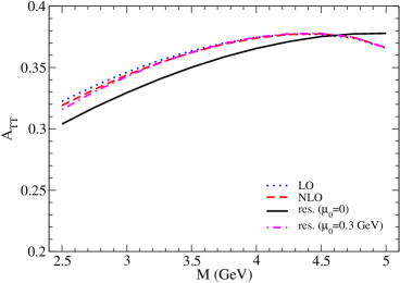
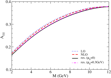
Figure 41: Corresponding spin asymmetries $A_{TT}(\phi=0)$ at LO, NLO and for the NLL resummed case.

D.3 Resummations and Nonperturbative Power Corrections

The measured spin asymmetry $A_{TT}$ can only be interpreted in terms of the transversity densities if the power corrections in (54) can either be shown to be small in the accessible kinematic domain, and/or if they are sufficiently well understood. There is a close relation between resummation and the nonperturbative power corrections. It has been shown that perturbative resummation suggests [13] the form of nonperturbative, power-suppressed, dynamics. There is reason to believe [11] that the large enhancement predicted by perturbation theory at $S=30$ GeV² (see Fig. 40) is only partly physical. As has been shown there, the very large corrections arise from a region where the resummed expression becomes sensitive to the behavior of the strong coupling at small scales. Further ongoing work focuses on the treatment of this “far-infrared” limit of resummed perturbation theory and its consequences.

D.4 Conclusions

Current work [11, 12] on the Drell-Yan cross section in the PAX kinematic regimes addresses NLO corrections, higher-order resummations, and also the study of nonperturbative power corrections. Large perturbative corrections to the Drell-Yan cross sections have been found which, however, cancel to a very large extent in the double-transverse spin asymmetry $A_{TT}$. Further studies aim to give an idea of the scale of non-perturbative power corrections. Studies performed so far suggest [11] that the Drell-Yan process is theoretically better understood for a GSI FAIR $\bar{p}p$ collider option than for the fixed-target case.

We finally emphasize that Drell-Yan measurements at PAX would allow us to enter uncharted territory in QCD: never before have precise Drell-Yan measurements been performed in this kinematic regime. Not only do we hope to learn about $A_{TT}$ and transversity. Also, measurements of the unpolarized cross section alone would shed light on the relationship between fixed orders, perturbative resummation and nonperturbative dynamics in hadronic scattering and thus enhance our understanding of QCD dynamics near the transition between the perturbative and nonperturbative regimes.

Part X Appendix E

Appendix E Beam Dynamics Simulations for the PAX using the BETACOOL code

E.1 Introduction

The simulations described in this appendix were carried out for the proton–antiproton collider mode of the PAX experiment using the CSR and the HESR The simulations made use of the RMS beam dynamics algorithm of the BETACOOL code [1]. The physical model of this algorithm is based on the following general assumptions:

1. the ion beam has a Gaussian distribution over all degrees of freedom, and this is not changed during the simulation;

2. the algorithm is considered to provide a solution of the equations for the RMS values of the beam phase space volume in three degrees of freedom, i.e. at this stage no tracking of individual particles is performed;

3. the maxima of all distribution functions coincide with the equilibrium orbit, all instability factors (linear and nonlinear resonances, space–charge effects, beam–beam tune shift, etc.) are not taken into account during the simulation.

The following effects are included in the simulation:

• Electron cooling (EC),

• Intrabeam scattering (IBS),

• Scattering on the residual gas (RG), and

• Particle losses (PL) from the hadronic interaction at the interaction point (IP).

The EC is taken into account using the Parkhomchuk model [5] of the friction force. The IBS growth rates are calculated with the Martini model [6] using ring lattice functions imported from the output file of the MAD program [3]. Interactions at the IP are used for the simulation of the luminosity and beam–beam parameters. The following PL effects were used during simulation: electron capture in EC for the proton beam, losses due to interactions at the IP with a total $\bar{p}p$ cross section of 40 mbarn, scattering on the residual gas (electron capture, single scattering, nuclear reactions).

The goal is to provide in the collider mode a luminosity in excess of $10^{30}$ cm^-2s^-1. In order to avoid the hourglass effect, the bunch lengths have to be about 30 cm, which is equal to the beta–functions at the IP. The parameters of the RF system are responsible to ensure a bunch length of 30 cm in equilibrium. The simulation for the collider mode was carried out for the highest energies achievable in each of the rings (HESR: 15 GeV/c, and CSR: 3.65 GeV/c). A list of initial parameters used in the simulation is given in Table 14.

The initial emittances of the proton and the antiproton beam in the collider mode were chosen such that the diameter of the ion beam is smaller than the diameter of the electron beam in the cooler section (Table 14). After equilibrium is reached, both the proton and the antiproton beam have approximately the same radius and bunch length at the collision point. The cooling rates in equilibrium are equal to the IBS growth rates.

The electron cooler for the HESR has the same design parameters as those required for experiments with a dense internal hydrogen pellet target of PANDA [2]. The electron cooler for the CSR requires a strong cooling force in order to provide cooling of the short proton bunches. The required length of the cooling section for the CSR is about 10 m, i.e. about 3 times longer than the 2 MV cooler to be built to provide a test bed for high energy electron cooling at COSY [4].

Initial Parameters	CSR	HESR
Particles	proton	antiproton
Momentum [GeV/c]	3.65	15
Relativistic factor $\gamma$	4.04	16.1
RF Harmonic Number	10	30
RF Voltage [kV]	200	200
Number of particles per bunch	$10^{11}$	$10^{10}$
Number of bunches	10	30
Beta function at IP [m]	0.3	1
Cross section at IP [mbarn]	40	40
Transverse emittance [mm mrad]	1	0.13
Momentum spread $\Delta P/P$	$10^{-3}$	$5\times 10^{-4}$
Electron Cooler
Cooler length [m]	10	30
Magnetic field [kG]	2	5
Beam radius [cm]	0.5	0.5
Beam current [A]	3	1
Horizontal beta function [m]	14	100
Vertical beta function [m]	14	100
Equilibrium Parameters
Beam parameter	$3\times 10^{-3}$	$6\times 10^{-3}$
Transverse emittance [mm mrad]	0.42	0.032
Momentum spread $\Delta P/P$	$2.5\times 10^{-4}$	$1.9\times 10^{-4}$
Bunch length [cm]	27	22
Transverse cooling/heating rate [$s^{-1}$]	0.059	0.012
Longitudinal cooling/heating rate [$s^{-1}$]	0.102	0.014
Cooling time [s]	$\approx 100$	$\approx 1500$
Peak luminosity [cm-2s-1]	$1.6\times 10^{30}$
Particle losses
Interaction point [s-1]	$6.5\times 10^{-8}$	$2.2\times 10^{-7}$
Electron Cooler [s-1]	$6.1\times 10^{-6}$	$1.2\times 10^{-7}$ ∗
Rest gas ($10^{-10}$ mbar) [$s^{-1}$]	$6.8\times 10^{-8}$	$1.3\times 10^{-7}$
Total beam life time [h]	$\approx 45$	$\approx 800$

Table 14: Initial parameters used in the simulation, parameters of the electron cooler, equilibrium parameters, and particle losses. (The particle losses in the electron cooler of the HESR (^∗) are calculated for protons, for antiprotons, this loss mechanism is absent.)

E.2 The Cooling Process

The behavior of the RMS beam parameters (emittance, momentum spread, bunch length, and luminosity) during the cooling process is presented in Fig. 42. The panels on the left side correspond to the CSR, those on the right to the HESR. The initial values are listed in Table 14. In the CSR, it takes about 200 s until the beam parameters reach equilibrium, while the in the HESR, a cooling time around 1500 s is required. After cooling, all parameters reach a constant value and do not change for a long time. Particle loss rates are a few order of magnitudes smaller than the cooling time and were not taken into account during the simulation.

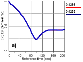
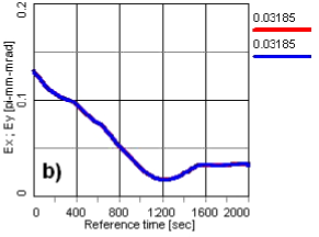
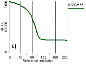
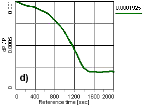
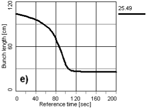
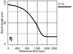
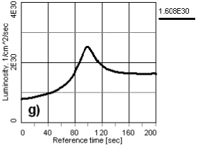
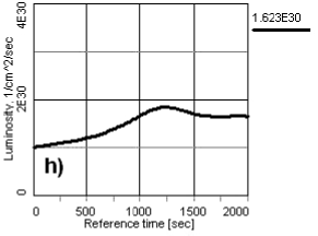
Figure 42: Results of the RMS beam dynamics calculation for CSR and HESR in the collider mode. The panels on the left side are for the CSR, those on the right for the HESR. From top to bottom, the panels denote the beam emittance, momentum spread, bunch length, and luminosity. The final numbers of each parameter are shown on the top right next to each panel.

The dip of the emittance and, respectively, of the luminosity as function of time can be explained with the help of three–dimensional diagrams, shown in Fig. 43, where the transverse emittance is shown as a function of the momentum spread. The vertical emittance is assumed to be equal to the horizontal one.

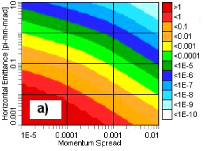
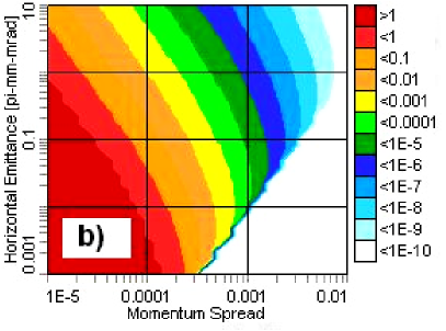
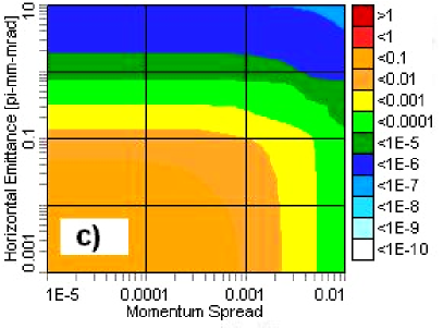
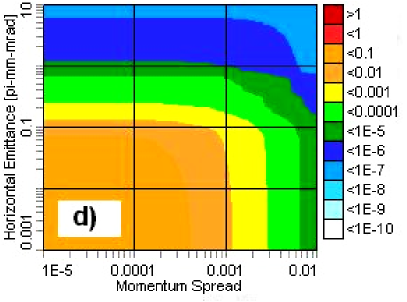
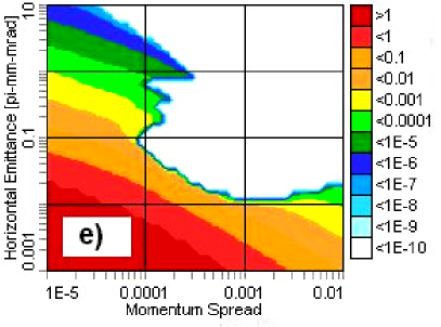
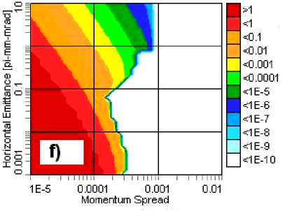
Figure 43: 3D diagrams of growth rates [s^-1] for the HESR as function of the momentum spread, in accordance with the RMS beam dynamics results, shown in Fig. 42. The panels on the left side apply to transverse, those on the right to longitudinal components. From top to bottom, the panels denote the IBS growth rates (a and b), cooling rates of the EC (c and d), and the combined effect of heating and cooling rates (e and f).

The cooling rates for the EC (Fig. 43, panels c and d) are calculated in accordance with the Parkhomchuk formula of the cooling force [5]. The transverse and longitudinal components of the cooling rates show approximately the same behavior. The combined effect of cooling and heating rates is presented in Fig. 43 (e and f). The boundaries between colored and white areas indicate the equilibrium between IBS and EC for the transverse and longitudinal components. The regions of the equilibrium can be found if one combines all four panels (a, b, c, and d) of Fig. 43, which results in Fig. 44. The final position of the equilibrium point does not depend on the initial coordinate.

In Fig. 44 the dependence of the transverse emittance on the momentum spread during the cooling process for the RMS dynamics of Fig. 42 (b and d) is shown.

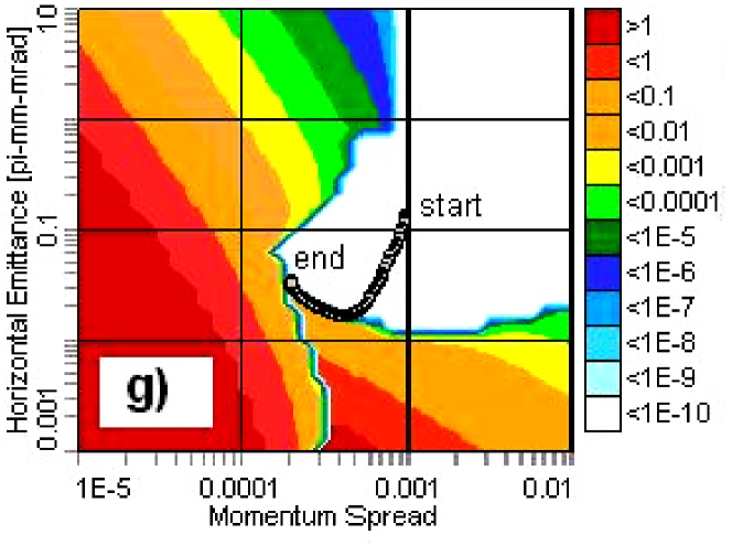
Figure 44: 3D diagram (transverse emittance vs momentum spread) of the transverse and longitudinal components of cooling and heating rates, arrived at by combining the panels e and f of Fig. 43 for the HESR. The open circles indicate the evolution of the beam parameters from a starting point (start) to the equilibrium point (end). The equilibrium point is unique, i.e. it does not depend on the particular choice of the starting point.

Initially, the electron cooling force achieves equilibrium with the transverse component of IBS. During this process, the emittance and the momentum spread are decreased. Subsequently, the cooling process continues and the beam parameters change in accordance with the equilibrium boundary of the transverse component. The momentum spread continues to decrease but the transverse emittance begins to increase. When the cooling force also reaches equilibrium with the longitudinal component of the IBS, the beam parameters converge to an equilibrium point, which does not depend on the initial parameters. The RMS dynamics is rather different and the cooling time can show large changes. This indicates that the initial parameters of the ion beam do not influence the equilibrium point but have a large effect on the cooling time.

E.3 Cycling of APR, CSR and HESR

The three rings, APR, CSR and HESR have to be operated together to provide the maximum luminosity for the collider experiments at the PAX experiment. A scheme showing how the three rings are cycled altogether, is shown in Fig. 45. Some details of the ring operation do not require much time, i.e. they are fast and do not affect the integrated luminosity. These are: injection, acceleration, bunching, and the cooling time. The following effects define the time table of experiment:

1. Production rate of antiprotons,

2. Polarization buildup time of antiprotons in the APR,

3. Space charge limit of particles at the injection energy, and

4. Beam lifetime in all storage rings.

The production rate of antiprotons is assumed to amount to about $10^{7}$ s^-1 ($=3.6\times 10^{10}$ h^-1). The polarization buildup time in the APR is defined by the lifetime of the antiproton beam in the interaction with the hydrogen target (see Sec. 8.2.2). In order to achieve the maximum polarization of about 0.4, a ring acceptance angle of $\psi_{\mathrm{acc}}=50$ mrad is required, which corresponds to a beam lifetime of $\tau_{\mathrm{APR}}=17$ h. The number of particles which can be injected into the APR at each injection is

$$N_{\bar{p}}=2\times R\times\tau_{\mathrm{APR}}=1.2\times 10^{12}\;.$$ (56)

This value is close to the space charge limit for the APR at the injection energy. After spin–filtering for two beam lifetimes, the number of antiprotons decreases by about one order of magnitude, i.e. to about $N_{\bar{p}}=10^{11}$.

Subsequently, antiprotons are injected into the CSR. After acceleration and bunching, the antiproton beam has 10 bunches with $10^{10}$ particles per bunch. Then antiprotons are injected into the HESR. The new fill should then be added to the antiprotons already circulating in the HESR, thus the antiproton beam should be decelerated to the injection energy. The antiprotons are then injected into the HESR, accelerated up to the experimental energy, and the cooling process can start.

At the same time, a proton beam with intensity $N_{\bar{p}}=10^{12}$ is injected into the CSR, which also corresponds to the space charge limit at injection energy. After acceleration and bunching of the proton beam, the electron cooler is switched on. After both beams are cooled down, colliding beam experiments can be started. The proton beam lifetime in the CSR is mainly defined by electron capture in the cooler section (Table 14). But this effect is absent for antiprotons in the HESR and the beam lifetime is defined by the total cross section at the IP and the residual gas pressure. The vacuum pressure at HESR should not exceed about $10^{-10}$ mbar.

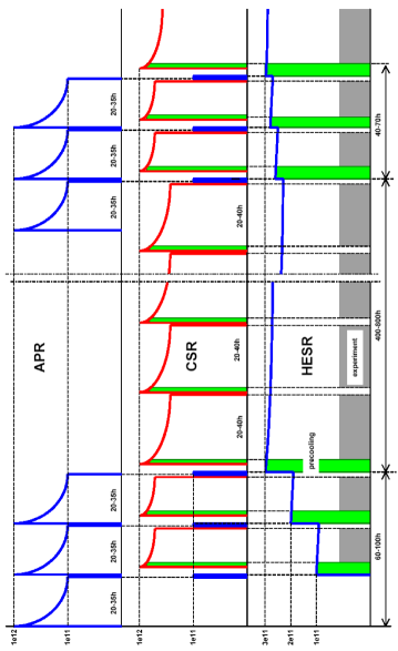
Figure 45: In the cycling scheme presented here, blue lines correspond to antiproton beam, red lines to proton beam . After the cooling process (green areas) in the CSR and in the HESR, the collider experiments can be started (black fill areas). The electron coolers stay in operation in both storage rings, CSR and HESR, to suppress intrabeam scattering during the experiments. Here we assume a conservative approach to the filling of the HESR. New fills from the APR are used to replace the antiprotons in the HESR with the largest dwell time.

The beam lifetime in the CSR is about one order of magnitude shorter less than in the HESR. The CSR should therefore be refilled with protons a couple of times, while antiprotons are circulated in the HESR. After the first injection of polarized antiprotons into the HESR, the experiments in the collider mode can be started. But the peak luminosity will be achieved only after injection of three cycles from the APR.

The cycling of the different rings for the PAX experiment is mainly defined by the lifetime of antiprotons in the HESR. After each cycle a new portion of antiproton beam replaces particles which were circulating in the ring before. In this scheme, the average luminosity is not so different from the peak luminosity. Because of the very long beam lifetime of the antiproton beam in the HESR ($\approx$ 800 h), in the collider mode antiprotons do not have to be delivered continously to the APR.

E.4 Possible Improvements

One way to increase the luminosity for PAX in the collider mode could consist of raising the injection energy in the CSR to avoid running into the space charge limit. But the lifetime of the antiproton beam is linearly proportional to the density of the proton beam. An increased proton beam intensity simply leads to a decrease of the beam lifetime of the antiproton beam.

Another option would be to increase the number of antiprotons in the HESR, which would lead to larger IBS growth rates and require longer cooling times. The time required to fill the HESR with antiprotons is linearly proportional to the particle number due to the fixed production rate of antiprotons. The estimate for the peak luminosity of ${\cal L}=1.6\times 10^{30}$ cm^-2s^-1 (listed in Table 14) is based on conservative assumptions about the number of antiprotons accumulated in the HESR. The number of antiprotons in the HESR can be increased by the transfer of more than just three shots from the APR, as depicted in Fig. 45. It should, however, be noted that the preparation (polarization buildup) of a single shot in the APR takes more than one day, thus the accumulation of ten shots in the HESR would take more than one week! In addition, any increase in the number of particles leads to larger instabilities due to space charge. In the present simulations, neither these effects nor instabilities due to resonances have been taken into account.

E.5 Summary

The present simulations show that in fact a high luminosity of ${\cal L}\approx 1.5\times 10^{30}$ cm^-2s^-1 in the collider mode can be achieved, however, to that end, a strong cooling force should be applied in both the CSR and the HESR. The parameters of the proton and antiproton beam are defined by the equilibrium between electron cooling and intrabeam scattering with values of heating growth rates of about 0.01–0.1 s^-1. The main particle loss mechanism in the CSR is electron capture in the cooler section. Particle losses in the HESR are mainly caused by scattering on the rest gas and by the hadronic interaction at the interaction point. The role of space–charge effects for the stability of the proton and antiproton beam should be further studied for the collider mode.

Part XI Appendix F

Appendix F Detector Simulation for PAX

F.1 PAX detector concept

The primary goal of this appendix to the PAX Technical Proposal is to show that the most challenging and outstanding measurement of the PAX experimental program, the direct measurement of the $h_{1}^{q}$ transversity distribution, is feasible. Moreover, the appendix is intended to show that other studies, like the measurement of the phases of the electromagnetic form factors of the proton and the spin correlations in the elastic proton-antiproton scattering, are much less demanding tasks, due to the high reaction rates involved.

An extensive program of studies has been started to investigate different options for the PAX detector configuration, aiming at an optimization of the achievable performance. We concentrate here on the detector design proposed in the PAX Technical Proposal (Fig. 46), which is well–suited to provide large invariant-mass $e^{+}e^{-}$ pair detection, from both Drell-Yan reactions and $\overline{p}p$ annihilations. In addition, such a detector is capable to efficiently detect secondaries in two body reactions, like elastic scattering events, where the over–constraint kinematics simplifies the event reconstruction and reduces the requirements for the particle identification. Alternative detector scenarios, e.g. based on $\mu^{+}\mu^{-}$ Drell–Yan pair detection, instrumented in the forward detector region or an extended hadron particle identification, will be studied at a later stage. The present detector is based on driving principles, outlined below.
The detector should:

• provide a large angular acceptance. Good azimuthal coverage and symmetry are needed to be sensitive to the dependence of the observables on the angle between production plane and target spin orientation. Several benchmark observables require an acceptance optmized for large polar angles, i.e. the $A_{TT}$ asymmetry in Drell-Yan reactions (Eq. 1) and the single ${\cal A}_{y}$ and double ${\cal A}_{yy}$, ${\cal A}_{zx}$ spin asymmetries in $\overline{p}p\rightarrow e^{+}e^{-}$ annihilations (Eq. 8) are weighted by trigonometric functions of the scattering angle, while the transverse spin effects on elastic scattering concentrate at large transverse momenta [1].

• be sensitive to electron pairs. Several detection tools allow one to efficiently identify electrons without an adverse effect on the momentum resolution. The overwhelming hadronic background requires excellent lepton identification. High momentum resolution is needed to be sensitive to $h_{1}$ dependence on Bjorken $x$; in addition it opens the interesting possibility to extend the measured range down to 2 GeV dilepton mass, thereby enlarging the Bjorken $x$ coverage of the $h_{1}$ measurement and facilitating the study of spin effects in the resonance production versus continuum region. A high resolution device with excellent particle identification constitutes a flexible and complete facility which can cope with new physics goals that may emerge in the upcoming years.

• use a toroid magnet. The spectrometer should provide high momentum resolution and measure the charge of secondaries. This is crucial in order to identify the wrong–charge control sample and subtract the combinatorial background. The spectrometer magnet should not affect the transverse spin orientation of the beam and provide an environment to ensure the operation of the Čerenkov detector. The toroid has almost negligible fringe-fields outside its active volume, both internally along the beam line and externally inside the tracking volume.

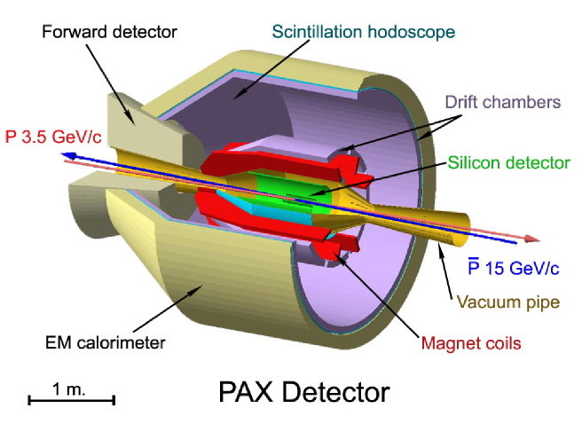
Figure 46: This conceptual design of the PAX detector is employed to estimate the performance of the detector and to show the feasibility of the transversity measurement in the asymmetric antiproton–proton collider mode at PAX. The artists view is produced by Geant.

F.2 Phase–I: Electromagnetic form factors of the proton and hard elastic scattering

This section presents the signal estimates for the benchmark measurements in Phase–I of PAX physics program. Here a (polarized) antiproton beam with momentum up to 3.6 GeV/c scatters off a polarized internal gas target in the CSR ring. The signal estimates show that the reaction rates are large enough to not put stringent requirements on the experimental set–up. The luminosity in fixed target mode is calculated as ${\cal L}=N_{\overline{p}}\cdot f\cdot d_{t}$ where $N_{\overline{p}}=10^{11}$ is the number of antiprotons stored in CSR, $f=L_{\rm CSR}/\beta_{\overline{p}}c\sim 1$ MHz is the antiproton revolution frequency depending on the antiproton velocity ($\beta_{\overline{p}}c$) and on the length of the CSR ring ($L_{\rm CSR}$), and $d_{t}=10^{14}$ $\rm cm^{-2}$ is the areal density of the target.

F.2.1 Electromagnetic form factors of the proton

Using the $p\overline{p}\rightarrow e^{+}e^{-}$ cross-section measured by PS170 [2] it is possible to estimate the running time required to get a precise measurement of the relative phases of the time–like electric and magnetic form–factors of the proton. For single spin asymmetries (SSA) and double spin asymmetries (DSA), the statistical error scales as

$$\Delta A_{\rm SSA}=\frac{1}{Q}\frac{1}{\sqrt{N_{\rm SSA}}}\hskip 56.9055pt\Delta A_{\rm DSA}=\frac{1}{QP}\frac{1}{\sqrt{N_{\rm DSA}}}$$

where $Q=0.8$ is the proton target and $P=0.3$ is the expected antiproton beam polarization. $N_{\rm SSA}$ ($N_{\rm DSA}$) is the number of collected events in the single (double) polarized mode. The following table lists the running time required to reduce the error down to $\Delta A=0.05$ for a few typical beam momenta, accessible in the CSR:

Beam	c.m. energy	$\sigma^{p\overline{p}\rightarrow e^{+}e^{-}}$	${\cal L}$	Running time	Running time
momentum	$\langle s\rangle$	PS170		DSA	SSA
(MeV/c)	($\rm GeV^{2}$)	(nbarn)	($\rm cm^{-2}s^{-1}$)	(days)	(days)
549	3.76	7.3	$7.8\cdot 10^{30}$	2.9	0.3
900	4.18	3.7	$1.1\cdot 10^{31}$	4.7	0.5
3600	8.75	0.044	$1.5\cdot 10^{31}$	132	13

Here a 50 % acceptance for $\sigma^{p\overline{p}\rightarrow e^{+}e^{-}}$ events is estimated basing on the conceptual PAX detector described in the previous section. Most of the measurements can be performed in a relatively short time, from less than 1 day up to few weeks. Only the most challenging measurement of double polarized asymmetries at the largest momenta requires a few months of data–taking. Note that the CSR ring be operated with polarized antiproton beam down to 200 MeV/c. Additional studies are foreseen to relax this limit and work even closer near threshold.

F.3 Hard elastic scattering

An estimate can be performed for the rate of hard $\overline{p}p$ elastic scatterings at the maximum transverse momentum achievable in the CSR. At the higher CSR antiproton beam energy of 3.6 GeV/c and at the largest scattering angles within the PAX detector acceptance (around $120^{\circ}$), the achievable momentum transfer is $t_{\rm PAX}=3.9$ $\rm GeV^{2}/c^{2}$. This is a benchmark experimental condition since there the cross–section is smallest, where one expects to observe the largest transverse spin effects. As a starting point we take the cross section measured by E838 at momentum transfer $t_{\rm E838}=5$ $\rm GeV^{2}/c^{2}$ [3]:

$$\left.\frac{d\sigma}{dt}\right|_{\rm E838}=10^{-4}\hskip 8.5359pt\frac{\rm mb}{\rm GeV}.$$

In a reasonable approximation the cross section scales with a tenth–power of the transverse momentum $t$, thus the E838 value can be rescaled to the PAX kinematics through

$$\left.\frac{d\sigma}{dt}\right|_{\rm PAX}=\left.\frac{d\sigma}{dt}\right|_{\rm E838}\cdot\left[\frac{t_{\rm E838}}{t_{\rm PAX}}\right]^{10}\sim 6\cdot 10^{-4}\hskip 8.5359pt\frac{\rm mb}{\rm GeV}.$$

Given the above estimated luminosity ${\cal L}=1.5\cdot 10^{31}$ $\rm cm^{-2}s^{-1}$, the event rate in a $\Delta t=0.1$ $\rm GeV^{2}/c^{2}$ interval, centered around the selected working point, is of the order of 1 Hz. The most challenging double–polarized measurement therefore requires only a few hours of data–taking to reach a precision of

$$\Delta A_{\rm DSA}=\frac{1}{QP}\frac{1}{\sqrt{N_{\rm DSA}}}=0.05.$$

F.4 Phase–II: The transversity measurement

The requirements to be fulfilled by the PAX detector have already been discussed in Sec. 15. Here we emphasize that the detector should be capable to cope with the overwhelming, $\sim 10^{7}$ times larger background than the Drell–Yan signal, and still should allow for reconstruction of the Drell–Yan kinematics with high resolution. A high resolution of the dilepton invariant–mass (and Feynman–$x_{F}$) allows one to efficiently isolate the resonance region from the continuum. Moreover, a precise determination of the Bjorken–$x$ of the proton and antiproton is important in order to maximize the sensitivity for the $x$–dependence of the $h_{1}^{q}(x)$ distribution function.

For these studies, the asymmetric–collider option, described in Sec. 7, was adopted as the most promising scenario, where a 15 GeV/c polarized antiproton beam from the HESR collides with a 3.5 GeV/c polarized proton beam from the CSR to produce $e^{+}e^{-}$ Drell-Yan events. In the following, we will label the Drell-Yan $e^{+}e^{-}$ candidate as right–sign dilepton pairs, whereas the background dilepton pairs, $e^{+}e^{+}$ and $e^{-}e^{-}$, will be labeled as wrong–sign dilepton pair.

F.4.1 Detector Simulation

Software
The proton-antiproton collisions are generated with the Pythia package implemented in Root. Particles generated from the interaction in antiproton–proton collisions are traced and particular detector responses are generated by the Geant 4 package. Whenever not explicitly stated, all physical processes regarding particles passing through the detector material, are accounted for in the simulation.

Data Samples
The interaction point was fixed at the origin of the coordinate system in order to maximize the detector acceptance in particular for the background events. Two data samples are generated:

Drell-Yan sample: it contains $10^{5}$ pure Drell–Yan events into electron–positron pairs. This sample is used to test the acceptance and resolution of the PAX detector.

Background sample: it consists of $2\cdot 10^{8}$ minimum–bias background events where Drell–Yan events and proton–antiproton elastic scattering events were excluded. This sample corresponds to about 40 minutes of data–taking with a cross-section of 40 mb and a luminosity of $2\cdot 10^{30}$ $\rm cm^{-2}s^{-1}$. The corresponding $e^{+}e^{-}$ Drell–Yan yield is of the order of 10 events.

Although the leptonic decays of charm resonances ($J/\Psi$ and $\Psi$) provide an alternative access to transversity [4], the simulation of these decays is not implemented yet.

Detector
The detector setup employed in the simulation is shown in Fig. 46: it consists of a somewhat simplified version of the one described in part IV, composed of a barrel section covering the $60^{\circ}$ to $120^{\circ}$ interval of polar angles, complemented by a detector part of conical shape, covering the smaller polar angles from $20^{\circ}$ to $60^{\circ}$. The right–handed coordinate system is defined as follows: the $z$–axis is pointing along the antiproton beam of 15 GeV/c momentum, $x$ points sideways, and the $y$–axis points upward. The origin of the coordinate system is located at the interaction point (IP).

Silicon detector (Si0, Si1): two layers of double–sided silicon strip detectors are placed close to the IP inside the vacuum of the beam pipe. They are utilized to measure the part of the track before the magnet, to reconstruct the vertex, and to veto neutral particles (especially gammas). The first layer has a thickness of 300 $\rm\mu m$ and a distance of 5 cm from the beam axes. The second layer has a thickness of 300 $\rm\mu m$ and a distance of 22 cm from the beam axes. The resolution is assumed to be 20 $\rm\mu m$ in both the longitudinal ($z$) and transverse ($R\phi$) coordinates [5].

Vacuum chamber (VC): the beam pipe connects with a vacuum chamber of 30 cm radius in correspondence with the IP. The windows of the vacuum chamber are made from a thin stainless–steel foil of 0.1 mm thickness.

Hodoscopes (H0, H1): two scintillation hodoscopes provide fast signals for triggering and time–of–flight information of low–momentum particles. The first scintillator, with a thickness of 4 mm, is placed just behind the vacuum window. The second one, with a thickness of 10 mm, is placed in front of the electromagnetic calorimeter.

Drift chambers (DC0, DC1): two drift chambers are placed at a distance of 65 and 135 cm from the beam axis to measure the track segments behind the magnet and to provide a momentum resolution of the order of 1 %. The assumed spatial resolution is 200 $\rm\mu m$ for both coordinates.

Čerenkov detector (CER): the detector is inserted into the free–space of the tracking arm of the drift chambers to provide an at least 60 cm thick radiator along the particle path. Since no particle–identification (PID) procedure is implemented into the simulation yet, the detector response is not generated. Nevertheless the detector material is accounted for during the particle tracking.

Calorimeter (EC): the electromagnetic calorimeter is a homogeneous detector with full azimuthal coverage and a length along the particle path extending up to 16 $X_{0}$, able to contain 5 GeV showers. In the present simulation it is assumed to consist of 14 cm long radiation–hard $\rm PbW0_{4}$ scintillator crystals. The response for electromagnetic particles ($e^{\pm}$ and $\gamma$) is parameterized by $\sigma_{E}/E=3\%/\sqrt{E}\oplus 0.5\%$ where $\oplus$ stands for summing in quadrature the two contributions [6]. All other particles are fully tracked inside the calorimeter material. Since the assumed resolution is achievable by other types of commonly used detectors, like lead glass or ionization calorimeters [7, 8, 9], the validity of the result is not limited to the scintillating material.

Spectrometer Magnet: the toroidal magnetic field for the momentum analysis of charged particles is generated by eight superconducting coils arranged symmetrically around the beam pipe. Each coil occupies a non–instrumented azimuthal sector of $5^{\circ}$. The acceptable solid angle is reduced by less than 11 % and ensures an azimuthal acceptance in excess of 80 % for Drell–Yan dilepton events. Although a coil design similar to the one of Atlas can be anticipated [10] and detailed studies on the realistic field map are in progress, the magnet details have not been taken into account yet in the simulation in order to save computing time. A homogeneous toroidal field is assumed with a total bending power of 0.4 Tm. Deep electromagnetic showers generated by the coil materials may prevent efficient event reconstruction within a time interval comparable with DC drift–time. Preliminary simulations have shown that the number of these showers is small enough to ensure a good detector performance.

Event Reconstruction
Track segments are constructed from the hits in the silicon layers (Si0 and Si1, inner segments before the magnet) and in the DC0 and DC1 (outer segments after passing the magnetic field). The impact point on the EC is assumed to correspond to the hit position in the DC2, located just in front of the calorimeter. Pattern recognition is simplified in directions perpendicular to the bending plane: only pairs of hits within an azimuthal $2^{\circ}$ interval are combined to form a track segment. Tracks from the inner segments are accepted if the minimal distance with the beam axis is smaller than 5 mm. In addition, inner and outer track segments should not differ by more than $2^{\circ}$ in azimuthal angle.

The outer segment should point to an electromagnetic cluster in the EC with an energy deposit of more than 300 MeV. This threshold is chosen to be above the one for minimum–ionizing particles (MIPs).

The Drell-Yan sample is simulated with the magnetic field turned on in order to test the momentum resolution of the detector. The large background sample is traced inside the detector without magnetic field and without drift chamber digitization to improve the speed of the simulation. In this case, the track is reconstructed using only an inner segment pointing toward an EC cluster, 300 MeV above threshold.

F.4.2 Background Evaluation

The major sources of background to the Drell–Yan process are the combinatorial background from Dalitz–decays ($\pi^{0}$, $\eta$) and gamma conversions, which can be studied and subtracted using the wrong–sign candidates, and the decays of charmed–mesons, which can be studied and reduced by reconstructing the secondary vertex of the decays.

Light meson decay: electron prongs from mesons decaying in flight are rejected by requiring that the track points when extended backwards towards the IP d not appear in the bending plane. Fast Dalitz decays (mainly $\pi^{0}$) appear to originate directly from the interaction point. Dileptons from the decay of one single light meson, can be identified by their low invariant mass. Only multiple decays may generate a dilepton with invariant mass larger than 2 $\rm GeV/c^{2}$. Although an additional electromagnetic particle in the event can be used to identify the parent $\pi^{0}$ and to reject the candidate, this kind of request is not implemented yet into the simulation: the result can be considered as conservative. Due to its combinatorial origin, this background can be studied and subtracted at large invariant mass by investigating wrong–sign candidates (control sample).

Gamma conversion: gamma conversions are vetoed requiring a charged hit in the first silicon layer, belonging to an electron candidate track. To reject conversions taking place before or inside the first tracking layer, one may in addition require silicon hits with a twice as large energy deposit or the second prong of the lepton pair to be reconstructed by the DC. In the present simulation, only the veto from the first silicon layer is implemented, providing a conservative result. The background from gamma conversions has a combinatorial origin like the one from meson decay. Hence, the residual background can be finally subtracted using wrong–sign control sample.

Decay of charmed mesons: due to their associated production, large mass and short lifetime, charmed–mesons tend to produce dangerous right–sign candidates at high invariant mass. In the fixed–target mode, the center–of–mass energy is too low to generate a significant contamination from charmed mesons. At the higher collider energies, charm background may become a serious issue. This kind of background can be studied and eventually reduced by reconstructing the secondary vertex of the decay with the silicon detector. As an example, we note that the Babar vertex detector was already successfully employed to study $D^{0}-\overline{D}^{0}$ mixing, by measuring the vertex distribution of semileptonic decays of $D$ mesons  [11]. Charm background was accounted for in the present simulation, but no criteria were adopted yet to reduce it.

Misidentifications: The PAX detector is designed to provide redundant high–level information about the particle type. This includes a signal above threshold in the Čerenkov detector, a close to one $E/p$ ratio (between the energy $E$ deposited in the EC and the momentum $p$ measured in the spectrometer), a compact lateral profile of the EC cluster. In addition $dE/dx$ measurements in the tracking system and time–of–flight information can be eventually employed. In the present simulation, the background by particle misidentification is assumed to be negligible and neglected.

The dielectron invariant mass distribution for the background sample ($2\cdot 10^{8}$ minimum-bias $p\overline{p}$ interactions) is shown in Fig. 47.

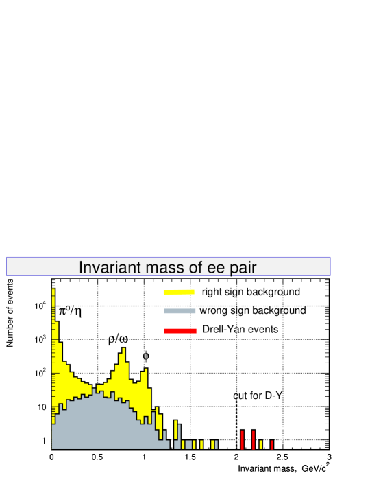
Figure 47: Background estimate for the PAX collider mode: right–sign background (yellow histogram) is dominated by single meson decay at low invariant mass. At high invariant mass the major component has combinatorial origin and can be subtracted by investigating the wrong–sign background (gray histogram). Here electron tracks with energy greater than 300 MeV should originate close to the beam axis; gamma conversions are vetoed by requiring a charged hit in the first silicon layer. PID and tracking system is assumed. One background event is found above the threshold imposed to Drell-Yan candidates, $M_{ee}=2$ $\rm GeV/c^{2}$. The generated statistics is $2\cdot 10^{8}$ $\overline{p}p$ inelastic interactions (40 minutes of data taking at a luminosity of $2\cdot 10^{30}$ $\rm cm^{-2}s^{-1}$). The corresponding yield of $e^{+}e^{-}$ Drell–Yan events inside the PAX detector acceptance is of the order of several events (red histogram). Although limited in statistics, this result supports the expectation of a signal over background ratio close to one before background subtraction. This is in agreement with what was anticipated in the TP basing on a simplified simulation without detailed detector description.

At low invariant mass, the right–sign candidates are dominated by the not–dangerous contribution from single meson decays [12]. This is indicated by the peaks in the distribution due to the high mass–resolution. The combinatorial background becomes the largest background source at dilepton masses larger than 1 $\rm GeV/c^{2}$. There it can be studied and subtracted by means of the wrong–sign control sample. Within the available statistics of $2\cdot 10^{8}$ $p\overline{p}$ collisions, the excess of right–sign candidates at large invariant masses due to the charm background is hardly visible. One background event is found with invariant mass above 2 $\rm GeV/c^{2}$. The corresponding Drell–Yan dielectron signal, inside the PAX detector acceptance with a mass greater than 2 $\rm GeV/c^{2}$, is expected to be of the order of several events. Note that the signal over background ratio is of the order of one before combinatorial background subtraction. Although limited in statistics, this study supports the view that the background for the $e^{+}e^{-}$ Drell-Yan measurement is well under control.

F.4.3 Detector Performance

For every Drell–Yan event, the Bjorken $x_{1}$ of the proton and $x_{2}$ of the antiproton can be extracted from the measured invariant mass ($x_{1}x_{2}s=M^{2}=Q^{2}$) and from the longitudinal momentum ($x_{1}-x_{2}=x_{F}=2p_{L}/\sqrt{s}$) of the lepton pair, where $s$ is the center–of–mass energy, as shown in Fig. 48.

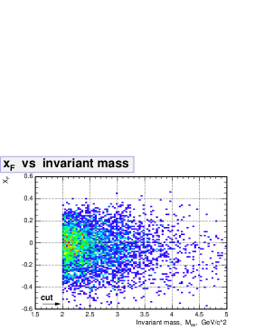
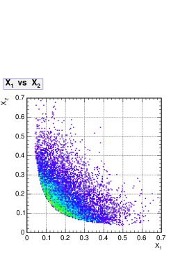
Figure 48: Kinematic distribution of the Drell–Yan events with $M_{ee}>2$ $\rm GeV/c^{2}$: Feynman $x_{F}=x_{1}-x_{2}$ versus invariant mass $M_{ee}=\sqrt{x_{1}x_{2}s}$ (left panel) and Bjorken $x_{2}$ versus $x_{1}$ (right).

In the $u$ dominance hypothesis, the $A_{TT}(x_{1},x_{2})$ asymmetry is related to the convolution of the transversity distributions $h_{1}^{u}(x_{1})\cdot h_{1}^{u}(x_{2})$ of the proton through the relation

$$A_{TT}(x_{1},x_{2})=\hat{a}_{TT}\;\frac{h_{1}^{u}(x_{1})}{u(x_{1})}\frac{h_{1}^{u}(x_{2})}{u(x_{2})}\hskip 56.9055pt\hat{a}_{TT}=\frac{\sin^{2}\theta}{1+\cos^{2}\theta}\cos(2\phi)\;.$$ (57)

where $u(x)$ is the up-quark unpolarized distribution and $\hat{a}_{TT}$ is the asymmetry of the elementary process $q\overline{q}\rightarrow e^{+}e^{-}$. The transverse asymmetry vanishes at small polar angles $\theta$. Moreover, the background from generic $p\overline{p}$ interactions concentrates in forward direction (Fig. 49).

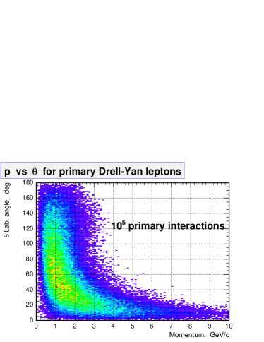
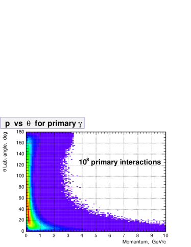
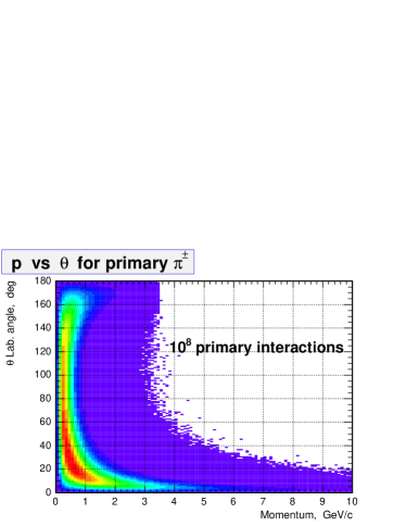
Figure 49: Phase space of Drell–Yan and background events: polar angle $\theta$ versus momentum $p$ of electrons (top left panel ) gamma (top right) and pions (bottom). Background particles concentrate at low energy and in the forward direction.

In the present simulation the PAX detector is not instrumented in the forward region, where the sensitivity to the $h_{1}^{u}$ is small. The active area of the detector is assumed to cover polar angles between $20^{\circ}$ and $120^{\circ}$. Although this reduces the acceptance for Drell–Yan events by about 50 %, it maximizes the sensitivity to the $h_{1}^{u}$ signal. The coils of the toroid cover only 11 % of the azimuthal acceptance. They are located outside of the $\phi=n\cdot\pi/2$ positions where the transverse asymmetry reaches its maximum.

A resolution of the order of 1 % in the lepton momentum and below 2 % in the dilepton invariant mass is achievable with the PAX spectrometer employing a magnetic bending power of 0.4 Tm, as shown in Fig. 50.

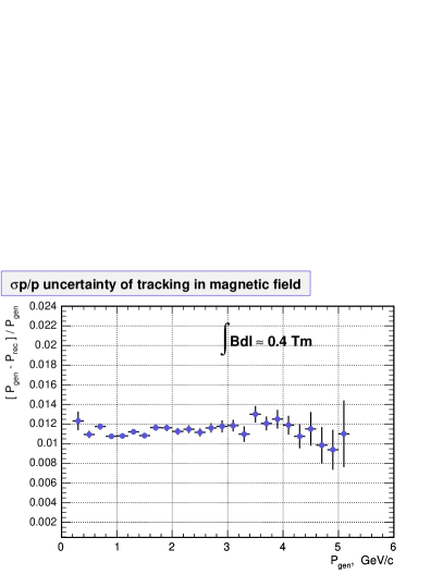
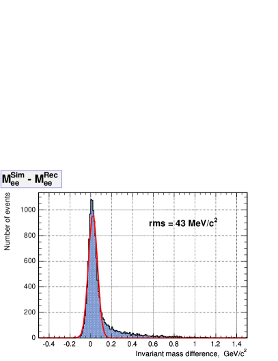
Figure 50: A 1 % resolution in the particle momentum (left panel) and a better than 2 % resolution in the dilepton invariant mass (right panel) are achievable by PAX spectrometer with a 0.4 Tm integrated field.

Such a resolution is required to efficiently distinguish the resonant contribution from the continuum contribution and to precisely extract the dependence of the $h_{1}^{u}$ distribution on the relevant kinematic variables (the Bjorken $x$ and the square of the four-momentum transfer $Q^{2}$). The silicon detector provides a $\sim 70$ $\rm\mu m$ resolution on the vertex position (Fig. 51). This value is in agreement with the design performance of the similar Babar silicon detector [5].

The Drell–Yan process is the reaction with the highest demand on luminosity among the ones proposed to be studied by PAX. The experimental uncertainty for double–spin asymmetries depends on the number of observed events $N$ as well as on the degrees of polarization of the two beams. A value of $P_{p}\mathrel{\hbox to0.0pt{\lower 4.0pt\hbox{\hskip 1.0pt$\sim$}\hss}\raise 1.0pt\hbox{$>$}}0.80$ can be assumed for the proton beam polarization, whereas values of $P_{\bar{p}}~{}\approx~{}0.30$ are anticipated for the antiproton beam polarization [13]. The statistical error of the transverse asymmetry $A_{TT}$ is then roughly given by $(P_{p}P_{\bar{p}}\sqrt{N})^{-1}=4/\sqrt{N}$. At a luminosity ${\cal L}=2\cdot 10^{30}$ $\rm cm^{-2}s^{-1}$, the expected signal rate is several hundreds of events per day inside the PAX detector acceptance. During one year of data–taking with the above assumed luminosity, the statistical error reduces to about 0.015. This uncertainty must be compared to the value of the measurable asymmetry which is ten times larger, of the order of $A_{TT}\sim\langle\hat{a}_{TT}\rangle\cdot 0.3\sim 0.15$. Here an indicative $A_{TT}/\hat{a}_{TT}=0.3$ value is assumed being supported by theoretical predictions [4, 14], whereas $\langle\hat{a}_{TT}\rangle\sim 0.5$ is the average value inside the PAX detector acceptance. It should be noted that an extensive study is foreseen to optimize the spin–filtering process: any beam polarization acquired in addition in the antiproton beam leads to a linear reduction of the experimental uncertainty.

The achievable precision of the ratio of the transverse $h_{1}^{u}(x)$ to the well–known unpolarized $u(x)$ distributions of the proton, in different intervals of Bjorken–$x$ and after one year of data–taking is shown in Fig. 52.

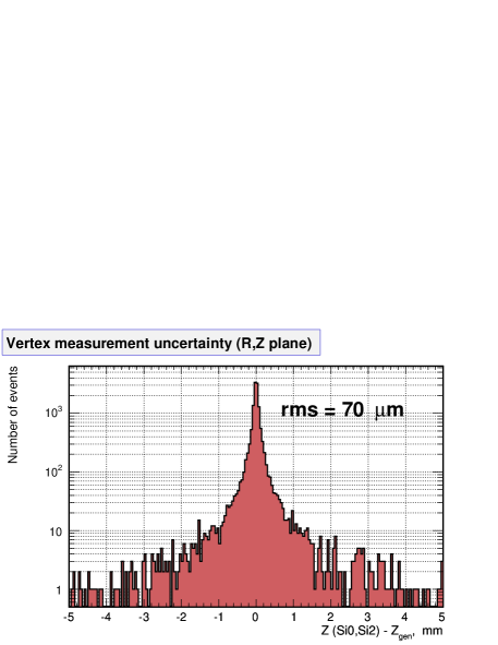
Figure 51: Resolution in the vertex position achievable with the PAX silicon detector. As demonstrated by Babar [11], this resolution is sufficient to study secondary vertices of charm–meson decays.

Figure 52: Expected precision of the $h_{1}^{u}(x)$ measurement for one year of data taking in the collider mode at PAX. A luminosity of $2\cdot 10^{30}$ $\rm cm^{-2}s^{-1}$ and a polar angle acceptance between $20^{\circ}$ and $120^{\circ}$ were assumed. An indicative $A_{TT}/\hat{a}_{TT}=0.3$ value (supported by theoretical predictions [4, 14]) is used as input to the simulation. The data points are plotted along the corresponding value of the $h_{1}^{u}(x)/u(x)$ ratio. The precision achievable within the full $Q^{2}>4$ $\rm GeV^{2}$ kinematic range is of the order of 10 % (top panel). The bottom panel shows the precision achievable in the restricted $Q^{2}>16$ $\rm GeV^{2}$ range. By tuning the beam energies, it should be possible to explore with high precision different $x$–intervals (see text).

The $h_{1}^{u}(x)$ transverse distribution can be measured in a wide $x$ range, from $x=0.7$ down to $x=0.05$, covering the most interesting valence region and extending to low values of $x$, where the theoretical predictions show the largest deviations. It should be noted that in principle the beam energies can be tuned to best explore different $x$ intervals. Indeed the highest sensitivity is achievable for $x\sim 1/\sqrt{p_{p}p_{\overline{p}}}$ (the center–of–mass energy $s\sim 4p_{p}p_{\overline{p}}$, and the Drell-Yan cross section peaks at low invariant masses of $M=\sqrt{x_{1}x_{2}s}\sim 2$ $\rm GeV/c^{2}$). These numbers entail only the non–resonant contribution to the Drell–Yan process: the exploitation of the $J/\Psi$ resonance region will lead to a considerable enhancement of the number of events in the $M^{2}$ = 9–16 GeV² range.

F.5 Summary

Extensive studies have been started to investigate different options for the PAX detector configuration, aiming at an optimization of the achievable performance.

F.5.1 Phase-I

In the Phase–I of the PAX physics program, where a (polarized) antiproton beam with momentum up to 3.6 GeV/c scatters off a polarized internal gaseous target, a luminosity of $1.5\cdot 10^{31}$ $\rm cm^{-2}s^{-1}$ can be safely achieved. Estimations of the expected signals show that

• the benchmark measurements of Phase–I, like the relative phases of electric and magnetic form factors of the proton or transverse spin effects in hard elastic scatterings, have no limiting reaction rates (see Fig. 53).

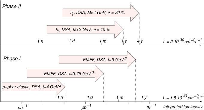
Figure 53: Integrated luminosities required to precise measure double–spin asymmetries (DSA) for the benchmark physics cases of the PAX program. The corresponding running time (h=hour, d=day, m=month, y=year) is indicated, as a function of the expected luminosity in Phase–I (fixed target, ${\cal L}=1.5\cdot 10^{31}$ $\rm cm^{-2}s^{-1}$) and in Phase–II (collider, ${\cal L}=2\cdot 10^{30}$ $\rm cm^{-2}s^{-1}$). An antiproton beam polarization of $P_{\overline{p}}=0.3$ and a proton polarization of $P_{p}=0.8$ are assumed. In Phase–I, polarized hard elastic scattering observables can be measured in a few hours of data–taking with an absolute error of $\Delta=0.05$, whereas the different measurements of the proton electromagnetic form factors entail from a few days up to a few months of data–taking to reach the same precision. In Phase–II, one year of running is enough to achieve a relative error of 10 % for the transversity distribution, if dilepton invariant masses larger than 2 GeV are accepted. In a few years, the $h_{1}$ measurement can be refined in the same mass range and verified with a relative error of 20 % at a higher mass scale, larger than 4 GeV and above the charm resonances.

F.5.2 Phase–II

The primary goal was to prove that the most challenging and outstanding measurement of the PAX experimental program, the direct measurement of the $h_{1}^{q}$ transversity distribution, is feasible. The asymmetric–collider option, described in Sec. 7 of the PAX Technical Proposal, was adopted as the most promising scenario, where a 15 GeV/c polarized antiproton beam from the HESR collides with a 3.5 GeV/c polarized proton beam from the CSR to produce $e^{+}e^{-}$ Drell-Yan events. A detailed simulation of the performances of the detector proposed in the PAX Technical Proposal, which is designed to provide $e^{+}e^{-}$ Drell–Yan pair detection, has been performed. Although preliminary, the results are very encouraging:

• the background is under control and can be studied with control samples: in particular the signal over background ratio is expected to be of the order of one but the major background component, being of combinatorial origin, can be subtracted by means of the measured wrong-sign candidates;

• a vertex detector similar to already working devices can provide a resolution in the vertex position better than 100 $\rm\mu m$: this is useful to control background from charm–meson decays;

• conventional tracking detectors can provide a resolution better than 2 % in dilepton invariant mass: this is sufficient to efficiently distinguish resonance from continuum contributions and to investigate the $h_{1}^{q}(x)$ dependence. As a consequence, the requirements on the calorimeter performance can be relaxed and solutions cheaper than scintillating devices can be investigated;

• during one year of data–taking, the most interesting valence region can be explored and the $h_{1}^{q}$ transverse distribution can be measured with a precision better than 10 %.

A conservative estimate of the luminosity achievable in the accelerator scheme presented in the PAX Technical Proposal, (and described in Appendix E) provides a value around $2\cdot 10^{30}$ $\rm cm^{-2}s^{-1}$. With this luminosity, a few years of data-taking would be sufficient to obtain a definite measurement of the last leading piece of the partonic description of the nucleon (Fig. 53).

References

- [1] A comprehensive review paper on the transverse spin structure of the proton can be found in: V. Barone, A. Drago and P. Ratcliffe, Phys. Rep. 359 (2002) 1.
- [2] M. Anselmino, V. Barone, A. Drago and N.N. Nikolaev, Phys. Lett. B594 (2004) 97.
- [3] A. Efremov, K. Goeke and P. Schweitzer, Eur. Phys. J.C35 (2004) 207.
- [4] D. Sivers, Phys. Rev. D41 (1990) 83; Phys. Rev. D43 (1991) 261.
- [5] J.C. Collins, Nucl. Phys. B396 (1993) 161.
- [6] HERMES Collaboration, A. Airapetian et al., Phys. Rev. Lett. 84 (2000) 4047; Phys. Rev. Lett. 90 (2003) 092002; Phys. Rev. D64 (2001) 097101; K. Rith, Progress in Part. and Nucl. Phys. 49 (2002) 245.
- [7] A. Airapetian et al., [HERMES Collaboration], Phys. Rev. Lett. 94 (2005) 012002.
- [8] J.C. Collins, Phys. Lett. B536 (2002) 43.
- [9] M. K. Jones et al., [Jefferson Lab Hall A Collaboration], Phys. Rev. Lett. 84 (2000) 1398. O. Gayou et al., [Jefferson Lab Hall A Collaboration], Phys. Rev. Lett. 88 (2002) 092301; Phys. Rev. C 64 (2001) 038202.
- [10] A. Z. Dubnickova, S. Dubnicka, and M. P. Rekalo, Nuovo. Cim. A 109 (1966) 241.
- [11] S. J. Brodsky, C. E. Carlson, J. R. Hiller and D. S. Hwang, Phys. Rev. D 69 (2004) 054022.
- [12] For a discussion on the validity of continuing space–like form factors to the time–like region, see, B. V. Geshkenbein, B. L. Ioffe, and M. A. Shifman, Sov. J. Nucl. Phys. 20 (1975) 66 [Yad. Fiz. 20 (1974) 128]; T. Gousset and B. Pire, Phys. Rev. D51 (1995) 15.
- [13] H.–W. Hammer, U.–G. Meißner and D. Drechsel, Phys. Lett. B385 (1996) 343; H.–W. Hammer and U.–G. Meißner, Eur. Phys. J A20 (2004) 469.
- [14] E. Tomasi–Gustafsson and M.P. Rekalo, Phys. Lett. B504 (2001) 291.
- [15] V. Matveev et al., Lett. Nuovo Cimento 7 (1972) 719.
- [16] S. Brodsky and G. Farrar, Phys. Rev. Lett. 31 (1973) 1153 and Phys. Rev. D11 (1973) 1309.
- [17] M. Diehl, T. Feldmann, R. Jakob and P. Kroll, Phys. Lett. B460 (1999) 204.
- [18] P. Landshoff, Phys. Rev. D10 (1974) 1024; P. Landshoff and D. Pritchard, Z. Phys. C6 (1980) 69.
- [19] J.P. Ralston and B. Pire, Phys. Rev. Lett. 61 (1988) 1823; ibid. 49 (1982) 1605; Phys. Lett. B117 (1982) 233.
- [20] G. P. Ramsey and D. W. Sivers, Phys. Rev. D52 (1995) 116; Phys. Rev. D47 (1993) 93; Phys. Rev. D45 (1992) 79.
- [21] D. Dutta and H. Gao, arXiv:hep-ph/0411267.
- [22] P. Kroll and W. Schweiger, Nucl. Phys. A503 (1989) 865.
- [23] T.A. Armstrong et al., Phys. Lett. B385 (1996) 479.
- [24] K. Krueger et al., Phys. Lett. B459 (1999) 412.
- [25] D.L. Adams et al., Phys. Lett. B264 (1991) 462; A. Bravar et al., Phys. Rev. Lett. 77 (1996) 2626.
- [26] J. Adams et al. [STAR Collaboration], Phys. Rev. Lett. 92 (2004) 171801
- [27] M. Anselmino, M. Boglione, U. D’Alesio, E. Leader and F. Murgia, Phys. Rev. D71 (2005) 014002.
- [28] W. Vogelsang, “QCD spin physics: Status, and prospects for RHIC,” Pramana 63 (2004) 1251 [arXiv:hep-ph/0405069].
- [29] V. Barone, T. Calarco and A. Drago, Phys. Rev. D56 (1997) 527.
- [30] O. Martin, A. Schäfer, M. Stratmann and W. Vogelsang, Phys. Rev. D57 (1998) 3084; Phys. Rev. D60 (1999) 117502.
- [31] A. Bianconi and M. Radici, e-Print Archive: hep-ph/0412368.
- [32] M.J. Corden et al., Phys. Lett. B98 (1981) 220.
- [33] E. Anassontzis et al., Phys. Rev. D38 (1988) 1377.
- [34] P.L. McGaughey, J.M. Moss and J.C. Peng, Ann. Rev. Nucl. Part. Sci. 45 (1999) 217.
- [35] A. Mukherjee, M. Stratmann and W. Vogelsang, Phys. Rev. D 67 (2003) 114006.
- [36] V. Barone, C. Corianò, M. Guzzi and P. Ratcliffe, in preparation.
- [37] U. D’Alesio, private communication
- [38] M. Anselmino, M. Boglione, U. D’Alesio, E. Leader and F. Murgia, Phys. Rev. D70 (2004) 074025.
- [39] A.V. Efremov and O.V. Teryaev, Phys. Lett. B150 (1985) 383.
- [40] J.W. Qiu and G. Sterman, Phys. Rev. Lett. 67 (1991) 2264.
- [41] S.J. Brodsky, D.S. Hwang and I. Schmidt, Phys. Lett. B530 (2002) 99.
- [42] M. Burkardt, Phys. Rev. D66 (2002) 114005.
- [43] N. Hammon, O. Teryaev and A. Schäfer, Phys. Lett. B390 (1997) 409.
- [44] D. Boer, P.J. Mulders and O. Teryaev, Phys. Rev. D57 (1998) 3057.
- [45] D. Boer and P.J. Mulders, Nucl. Phys. B569 (2000) 505.
- [46] D. Boer and J. Qiu, Phys. Rev. D65 (2002) 034008.
- [47] M. Anselmino, U. D’Alesio and F. Murgia, Phys. Rev. D67 (2003) 074010.
- [48] A.V. Efremov, K. Goeke, S. Menzel, A. Metz and P. Schweitzer, Phys. Lett. B612 (2005) 233.
- [49] R. Baldini, S. Dubnicka, P. Gauzzi, S. Pacetti, E. Pasqualucci, and Y. Srivastava, Eur. Phys. J. C11 (1999) 709; R. Baldini et al., Proc. of the Physics at Intermediate Energies Conference ed. Diego Bettoni, eConf C010430, T20 (2001) [hep–ph/0106006].
- [50] See also R. Calabrese, in Proc. of the Physics at Intermediate Energies Conference ed. Diego Bettoni, eConf C010430, W07 (2001); H. W. Hammer, ibid., W08 (2001) [arXiv:hep–ph/0105337]; Carl E. Carlson, ibid., W09 (2001) [arXiv:hep–ph/0106290]; M. Karliner, ibid., W10 (2001) [arXiv:hep–ph/0108106].
- [51] M. Andreotti et al., Phys. Lett. B559 (2003) 20.
- [52] A. V. Belitsky, X. Ji, and F. Yuan, Phys. Rev. Lett. 91 (2003) 092003.
- [53] S. J. Brodsky, J. R. Hiller, D. S. Hwang and V. A. Karmanov, Phys. Rev. D 69 (2004) 076001
- [54] F. Iachello, A. D. Jackson, and A. Lande, Phys. Lett. B43 (1973) 191.
- [55] A. Kaidalov, L. Kondratyuk and D. Tchekin, Phys. Atom. Nucl. 63 (2000) 1395.
- [56] S. Dubnicka and A.-Z. Dubnickova, Fizika B 13 (2004) 287 [e–Print Archive: hep-ph/0401081].
- [57] R. Bijker and F. Iachello, Phys. Rev. C 69 (2004) 068291; F. Iachello, Eur. Phys. J A 19 (2004) 29, and e–print Archive: nucl-th/031207.
- [58] S. Rock, Proc. of the Physics at Intermediate Energies Conference ed. Diego Bettoni, eConf C010430, W14 (2001) [hep–ex/0106084].
- [59] J. P. Ralston and P. Jain, hep–ph/0302043; J. P. Ralston, P. Jain, and R. V. Buniy, AIP Conf. Proc. 549 (2000) 302 [hep–ph/0206074].
- [60] G. A. Miller and M. R. Frank, Phys. Rev. c65 (2002) 065205; M. R. Frank, B. K. Jennings, and G. A. Miller, Phys. Rev. C54 (1996) 920.
- [61] A. Z. Dubnickova, S. Dubnicka, and M. P. Rekalo, Z. Phys. C 70 (1996) 473.
- [62] M. Ambrogiani et al., Phys. Rev. D60 (1999) 032002.
- [63] Z. Bai et al., Phys. Rev. Lett. 91 (2003) 022001.
- [64] K. Abe et al., Phys. Rev. Lett. 88 (2002) 181803.
- [65] K. Abe et al., Phys. Rev. Lett. 89 (2002) 151802.
- [66] A. Sibirtsev, J. Haidenbauer, S. Krewald, Ulf-G. Meissner and A.W. Thomas, e–print arXiv: hep-ph/0411386.
- [67] T.A.Armstrong et al., Phys. Rev. Lett. 70 (1992) 1212.
- [68] E. Tomasi–Gustaffson and M.P. Rekalo, e–print arXive:nucl-th/0307065.
- [69] S. J. Brodsky, in Exclusive Processes at High Momentum Transfer, Workshop Proceedings, May 15–18, 2002. Jefferson Lab, Newport News, Virginia, editors A. Radyushkin and P. Stoler, World Scientific, pp. 1–33; S. J. Brodsky and G.P. Lepage, in Advanced Series on Directions in High Energy Physics, v. 5 : Perturbative Quantum Chromodynamics, editor A.H. Mueller, World Scientific (1989), pp. 93–240.
- [70] X. D. Ji, Phys. Rev. Lett. 78 (1997) 610. X. D. Ji, Phys. Rev. D55 (1997) 7114.
- [71] A. V. Radyushkin, Phys. Lett. B380 (1996) 417.
- [72] THE QCD STRUCTURE OF THE NUCLEON (QCD–N’02): Proceedings. Edited by E. De Sanctis, W.–D. Nowak, M. Contalbrigo, V. Muccifora. Amsterdam, Netherlands, North–Holland, 2002. Nucl. Phys. A711 (2002).
- [73] S. L. Brodsky and J. R. Hiller, Phys. Rev. C 28 (1983) 475; for a review see C.E. Carlson, J.H. Hiller and R.J. Holt, Annu. Rev. Nucl. Part. Sci. 47 (1997) 395.
- [74] A. V. Efremov and A. V. Radyushkin, Phys. Lett. B94 (1980) 245.
- [75] G.P. Lepage and S.J. Brodsky, Phys. Rev. D22 (1980) 2157.
- [76] V. L. Chernyak, A. R. Zhitnitsky and V. G. Serbo, JETP Lett. 26 (1977) 594 [Pisma Zh. Eksp. Teor. Fiz. 26 (1977) 760]; V. L. Chernyak and A. R. Zhitnitsky, Phys. Rept. 112 (1984) 173.
- [77] L. Y. Zhu et al. [Jefferson Lab Hall A Collaboration], Phys. Rev. Lett. 91 (2003) 022003; H. Gao and L. Zhu, arXiv:nucl-ex/0411014.
- [78] P. Rossi et al. [CLAS Collaboration], Phys. Rev. Lett. 94 (2005) 012301
- [79] M. Mirazita et al. [CLAS Collaboration], Phys. Rev. C 70 (2004) 014005
- [80] C. G. White et al., Phys. Rev. D 49 (1994) 58.
- [81] M. Diehl, T. Feldmann, R. Jakob and P. Kroll, Eur. Phys. J. C8 (1999) 409.
- [82] V. Barone, M. Genovese, N. N. Nikolaev, E. Predazzi and B. G. Zakharov, Z. Phys. C58 (1993) 541.
- [83] J. L. S. Aclander et al., Phys. Rev. C 70 (2004) 015208.
- [84] H.A. Neal and H.B.Nielsen, Pys. Lett. B 51 (1974) 79.
- [85] B. Z. Kopeliovich and B. G. Zakharov, Z. Phys. C 43 (1989) 241.
- [86] G. C. Rossi and G. Veneziano, Nucl. Phys. B 123 (1977) 507; L. Montanet, G. C. Rossi and G. Veneziano, Phys. Rept. 63 (1980) 149.
- [87] S.E. Vance, M. Gyulassy and X.N. Wang, Phys. Lett. B (1998 45; V. T. Pop, M. Gyulassy, J. Barrette, C. Gale, X. N. Wang and N. Xu, arXiv:nucl-th/0407095; K. Itakura, Y. V. Kovchegov, L. McLerran and D. Teaney, Nucl. Phys. A 730 (2004) 160; A. Capella, Phys. Lett. B 542 (2002) 65;
- [88] K. Wijesooriya et al. [Jefferson Lab Hall A Collaboration], Phys. Rev. Lett. 86 (2001) 2975.
- [89] P. R. Cameron et al., Phys. Rev. D32 (1985) 3070. G. R. Court et al., Phys. Rev. Lett. 57 (1986) 507. D. G. Crabb et al., Phys. Rev. Lett. 60 (1988) 2351. F. Z. Khiari et al., Phys. Rev. D39 (1989) 45.
- [90] H.A. Neal, J.B. Kuah and H.B. Nielsen, Phys. Lett. B 439 (1998) 407.
- [91] J. P. Ralston and B. Pire, Phys. Rev. Lett. 57 (1986) 2330.
- [92] J. L. Cortes, B. Pire and J. P. Ralston, Z. Phys. C 55 (1992) 409; J. P. Ralston and B. Pire, AIP Conf. Proc. 223 (1991) 228.
- [93] S. J. Brodsky and G. F. de Teramond, Phys. Rev. Lett. 60 (1988) 1924; G. F. de Teramond, R. Espinoza and M. Ortega-Rodriguez, Phys. Rev. D 58 (1998) 034012.
- [94] C. Lechanoine–LeLuc and F. Lehar, Rev. Mod. Phys. 65 (1993) 47.
- [95] C. Quigg, Nucl. Phys. B34 (1971) 77.
- [96] D. P. Roy, J. Phys. G 30 (2004) R113
- [97] A. Mukherjee, I. V. Musatov, H. C. Pauli and A. V. Radyushkin, Phys. Rev. D67 (2003) 073014.
- [98] M. Diehl, T. Feldmann, R. Jakob and P. Kroll, arXiv:hep-ph/0408173.
- [99] L. Elouadrhiri, Nucl. Phys. A711 (2002) 154. S. Stepanyan et al. [CLAS Collaboration], Phys. Rev. Lett. 87 (2001) 182002.
- [100] V. A. Korotkov and W. D. Nowak, Eur. Phys. J. C23 (2002) 455.
- [101] M. Diehl, P. Kroll and C. Vogt, Eur. Phys. J. C26 (2003) 567. M. Diehl, P. Kroll and C. Vogt, Phys. Lett. B532 (2002) 99.
- [102] M. Artuso et al. [CLEO Collaboration], Phys. Rev. D50 (1994) 5484.
- [103] H. Hamasaki et al. [VENUS Collaboration], Phys. Lett. B407 (1997) 185.
- [104] P. Kroll, private communication.
- [105] B. Pire and L. Szymanowski, arXiv:hep-ph/0411387.
- [106] B. Pire and L. Szymanowski, arXiv:hep-ph/0504255.
- [107] A. Donnachie and P.V. Landshoff, Phys. Lett. B296 (1992) 227; J. R. Cudell et al., Phys. Rev. D65 (2002) 074024.
- [108] R. Jakob and P. Kroll, Z. Phys. A344 (1992) 87.
- [109] L.N. Bogdanova, O.D. Dalkarov and I.S. Shapiro, Ann. Phys. 84 (1974) 261.
- [110] I.S. Shapiro, Phys. Rept. 35 (1978) 129.
- [111] G.C. Rossi and G. Veneziano, Phys. Rep. 63 (1980) 153.
- [112] C.B. Dover, T. Gutsche and A. Faessler, Phys. Rev. C43 (1991) 379.
- [113] W. Grein, Nucl. Phys. B131 (1977) 255.
- [114] H. Kaseno et al., Phys. Lett. B61 (1976) 203.
- [115] C. Bourrely, J. Soffer and D. Wray, Nucl. Phys. B77 (1974) 386.
- [116] P. Jenni et al., Nucl. Phys. B94 (1975) 1.
- [117] R. Jakob and P. Kroll, Z. Phys. A344 (1992) 87.
- [118] J. Bystricky, F. Lehar, and P. Winternitz, J. Phys. 39 (1978) 1.
- [119] D. P. Grosnick et al. [E581/704 Collaboration], Phys. Rev. D55 (1997) 1159.
- [120] A. Gade ”The HERMES unpolarized gas feed system, Version 4.0” HERMES internal report (2003).
- [121] F. Rathmann et al., Phys. Rev. Lett. 71 (1993) 1379.
- [122] E. Klempt, F. Bradamante, A. Martin, and J.–M. Richard, Phys. Rep. 368 (2002) 119.
- [123] F. Rathmann et al., Phys. Rev. Lett. 94 (2005) 014801.
- [124] H.O. Meyer, Phys. Rev. E50 (1994) 1485.
- [125] C.J. Horowitz and H.O. Meyer, Phys. Rev. Lett. 72 (1994) 3981.
- [126] R. Madey et al., Phys. Rev. Lett. 91, 122002 (2003); S. Strauch et al., Phys. Rev. Lett. 91, 052301 (2003); O. Gayou et al., Phys. Rev. Lett. 88, 092301 (2002).
- [127] For a list of PAX collaboration meetings, conference presentations, QCD–PAC and STI reports, please visit the PAX web–site at http://www.fz-juelich.de/ikp/pax
-
[128]
ASSIA Letter–of–Intent, spokesperson: R. Bertini,
http://www.gsi.de/documents/DOC-2004-Jan-152-1.ps - [129] Proc. of the Workshop on Polarized Antiprotons, Bodega Bay, CA, 1985, Eds. A. D. Krisch, A. M. T. Lin, and O. Chamberlain, AIP Conf. Proc. 145 (AIP, New York, 1986).
- [130] D.P. Grosnick et al., Nucl. Instrum. Methods A290 (1990) 269.
- [131] H. Spinka et al., Proc. of the 8th Int. Symp. on Polarization Phenomena in Nuclear Physics, Bloomington, Indiana, 1994, Eds. E.J. Stephenson and S.E. Vigdor, AIP Conf. Proc. 339 (AIP, Woodbury, NY, 1995), p. 713.
- [132] T.O. Niinikoski and R. Rossmanith, Nucl. Instrum. Methods A255 (1987) 460.
- [133] P. Cameron et al., Proc. of the 15th Int. Spin Physics Symp., Upton, New York, 2002, Eds. Y.I. Makdisi, A.U. Luccio, and W.W. MacKay, AIP Conf. Proc. 675 (AIP, Melville, NY, 2003), p. 781.
- [134] K. Zapfe et al., Rev. Sci. Instrum. 66 (1995) 28.
- [135] K. Zapfe et al., Nucl. Instrum. Methods A368 (1996) 627.
- [136] V. Mull and K. Holinde, Phys. Rev. C 51, 2360 (1995).
- [137] Preservation of beam polarization is routinely accomplished at COSY–Jülich [196], and at higher energies at the AGS of BNL [157, 158, 159].
- [138] Ya. S. Derbenev et al., Part. Accel. 8, 115 (1978); A. Lehrach and R. Maier, Proc. of the 2001 Particle Accelerator Conference, Chicago, Illinois, 2001, Eds. P. Lucas and S. Webber, (IEEE, Piscataway, NJ, 2001), p. 2566.
- [139] W. Haeberli, Ann. Rev. Nucl. Sci. 17 (1967) 373.
- [140] A. Zelenski et al., Nucl. Instrum. Methods A, in press, available from http://www.sciencedirect.com/science/article/B6TJM-4D97J59-3/2/fa659e20fd61ea04fb72e77b82fa99ed.
- [141] E. Steffens and W. Haeberli, Rep. Prog. Phys. 66 (2003) 1887.
- [142] Particle Data Group, available from http://pdg.lbl.gov/2002.
- [143] G.G. Ohlsen and P.W. Keaton, Nucl. Instrum. Methods 109 (1973) 41.
- [144] C. Bovet et al., A Selection of Formulae and Data Useful for the Design of A.G. Synchrotrons, CERN/MPS-SI/Int. DL/70/4, 23 April (1970).
- [145] J.H. Malmberg et al., Non–neutral Plasma Physics, Eds. C.W. Roberson and C.F. Driscoll, (AIP, New York, 1988), p. 28.
- [146] J. Grames et al., see p. 1047 of ref [133].
- [147] S. Nagaitsev, private communication, EPAC 2004.
- [148] P.J. Bryant, AC Division, CERN, CH-1211, Geneva 23.
- [149] UGS Gerlinde Schultheis & Partner, Agency for Technology Transfer, Langenbernsdorf, Germany.
- [150] Maier R.,Nucl. Inst. and Meth. A 390 (1997) 1.
- [151] Gebel R., private communication.
- [152] COSY-SCL Design Update, Internal Report, FZ J lich, March 2002, edited by H. Jungwirth.
- [153] Schwarz V. et al., “EDDA as Internal High-Energy Polarimeter”, Proc. International Spin Physics Symposium SPIN 1998, Protvino, (published in World Scientific Singapore (1999)).
- [154] V. Derenchuk and A.S. Belov, “Recent Improvements in CIPIOS Intensity and Operation”, Proc. of the 9th International Workshop on Polarized Sources and Targets, 2001, Nashville, IN, USA, eds. V.P. Derenchuk and B. von Przewoski, p. 210 (World Scientific Singapore, 2002).
- [155] L. Äystö et al., An International Accelerator Facility for Beams of Ions and Antiprotons, Conceptual Design Report, GSI (2001).
- [156] L.H. Thomas, Phil. Mag. 3, 1 (1927); V. Bargman, L. Michel, V.L. Telegdi, Phys. Rev. Letters 2 (1959) 43.
- [157] F.Z. Khiari et al., Phys. Rev. D39 (1989) 45.
- [158] H. Huang et al., Phys. Rev. Lett. 73 (1994) 2982.
- [159] M. Bai et al., Phys. Rev. Lett. 80 (1998) 4673.
- [160] see http://www.agsrhichome.bnl.gov/RHIC/Spin.
- [161] B.B. Blinov et al., Phys. Rev. Lett. 81 (1998) 2906; B.B. Blinov et al., Phys. Rev. ST Accel. Beams 3 (2000) 104001. V.S. Morozov et al., Phys. Rev. Accel. Beams 4 (2001) 104002. B.B. Blinov et al., Phys. Rev. Lett. 88 (2002) 014801.
- [162] For the web–site of the SPIN@COSY collaboration, see http://www.fz-juelich.de/ikp/spin@cosy.
- [163] V. S. Morozov et al., Phys. Rev. ST Accel. Beams 7 (2004) 024002; M.A. Leonova et al., Phys. Rev. Lett. 93 (2004) 224801.
- [164] A. Piwinski, “Touschek Effect and Intrabeam Scattering”, in: A. W. Chao, M. Tigner (eds.), Handbook of Accelerator Physics and Engineering, World Scientific, Singapore, 1999.
- [165] C. Baumgarten et al., Nucl. Instrum. Methods A482 (2002) 606.
- [166] R. Engels et al., Rev. Sci. Instr. 74 (2003) 4607.
- [167] R.A. Kunne et al. Phys. Lett. B206 (1988) 557; R.A. Kunne et al. Nucl. Phys. B323 (1989) 1.
- [168] M. G. Albrow et al., Nucl. Phys. B37 (1972) 349.
- [169] R.E. Pollock, Phys. Rev. E55 (1997) 7606.
- [170] A.I Akhiezer and Y.B. Berestetskii, “Quantum Electrodynamics”, Monographs and Texts in Physics and Astronomy, Vol. XI, p. 504, ed. R.E. Marshak, Interscience Publishers, 1965.
- [171] R. Schleichert et al., IEEE Trans. Nucl. Sci. 50 (2003) 301.
- [172] M. Ambrogiani et al., (E835 Collaboration) Phys. Rev. D60 (1999) 032002.
- [173] G. Bardin et al., (PS170 Collaboration), Nucl. Instrum. Methods A259 (1987) 376.
- [174] Aubert et al., (Babar Collaboration), Nucl. Instrum. Methods A479 (2002) 1.
- [175] C. Garabatos et al., Nucl. Instrum. Methods A412 (1998) 38.
- [176] M. D. Mestayer et al., Nucl. Instrum. Methods A449 (2000) 81.
- [177] S. Bagnasco et al., Nucl. Instrum. Methods A424 (1999) 304.
- [178] M. Aizawa et al., Nucl. Instrum. Methods A499 (2003) 508.
- [179] G. Adams et al., Nucl. Instrum. Methods A465 (2001) 414.
- [180] L. Fabbietti et al., Nucl. Instrum. Methods A502 (2003) 256.
- [181] CMS Technical Design Report, CERN/LHCC 97-33, CMS TDR 4 (1997).
- [182] ALICE Technical Design Report, CERN/LHCC 99-4, ALICE TDR 2 (1999).
- [183] V. A. Batarin et al., Nucl. Instrum. Meth. A510 (2003) 248.
- [184] HERMES Collaboration: Techn. Design Report (1993) DESY-PRC 93/06.
- [185] T. A. Armstrong et al. Phys. Lett. B385 (1996) 479.
- [186] T. Rinckel et al., Nucl. Instrum. Methods A439 (2000) 117.
- [187] K. Ackerstaff et al., (HERMES Collaboration) Nucl. Instrum. Methods A417 (1998) 230.
- [188] S. Barsov et al., Nucl. Instrum. Methods A 462 (2001) 364.
- [189] L. Afanasyev et al., Nucl. Instrum. Methods A491 (2002) 376.
- [190] Y. Inoue et al., Eur. Phys. Journ. C18 (2000) 273 Methods A734 (2004) 78.
- [191] E. Anassontzis et al., Phys. Rev. D38 (1988) 1377, A. Baldit et al., Phys. Lett. B 332 (1994) 244, E. A. Hawker et al., Phys. Rev. Lett. 80 (1998) 3715.
- [192] M. Artuso et al., PSI-PR-89-05.
- [193] T. Akesson et al., Nucl. Instrum. Methods A 512 (1998) 200.
- [194] O. Busch, Nucl. Instrum. Methods A 525 (2004) 153.
- [195] S. H. Aronson et al., Nucl. Instrum. Methods A 499 (2003) 480.
- [196] A. Lehrach et al., see p. 153 of ref [133].

References

- [1] G. Breit, Phys. Rev. 34 (1929) 553.
- [2] A.I Akhiezer and Y.B. Berestetskii, “Quantum Electrodynamics”, Monographs and Texts in Physics and Astronomy, Vol. XI, §38, Eq. (38.10), ed. R.E. Marshak, Interscience Publishers, 1965.
- [3] L.D. Landau and E.M. Lifshitz, Course of Theoretical Physics, Vol. 4: V.B. Berestetskii, E. M. Lifshitz and L.P. Pitaevskii, Relativistic Quantum Theory, Part 1, par. 83. Pergamon Press, 1971.
- [4] J. Bystricky, F. Lehar and P. Winternitz, J. Phys. (France) 39 (1978) 1.
- [5] H.O. Meyer, Phys. Rev. E 50 (1994) 1485; C.J. Horowitz and H.O. Meyer, Phys. Rev. Lett. 72 (1994) 3981.
- [6] A.I. Akhiezer, L.N. Rosenzweig and I.M. Shmushkevich, Zh. Exp. Teor. Fiz. 33 (1957) 765 [Sov. Phys. JETP 6 (1958) 588].
- [7] A.M. Bincer, Phys. Rev. 107 (1957) 1434.
- [8] J.H. Scofield, Phys. Rev. 113 (1959) 1599.
- [9] J.H. Scofield, Phys. Rev. 141 (1966) 1352.
- [10] N. Dombey, Rev. Mod. Phys. 41 (1969) 236.
- [11] A.I. Akhiezer and M.P. Rekalo, Sov. Phys. - Doklady 13, 572 (1968).
- [12] D. R. Yennie, D. G. Ravenhall, and R. N. Wilson, Phys. Rev. 95 (1954) 500
- [13] L.D. Landau and E.M. Lifshitz, Course of Theoretical Physics, Vol. 4, Part 1: V.B. Beresteskii, E.M. Lifshitz and L.P. Pitaevskii, Relativistic Quantum Theory, par. 89. Pergamon Press, 1971.
- [14] M.J. Alguard eat al., Phys. Rev. Lett. 37 (1976) 1258.
- [15] M. Meyerhoff et al., Phys. Lett. B 327, 201–207 (1994).
- [16] D. Rohe et al., Phys. Rev. Lett. 83 (1999) 4257.
- [17] D. I. Glazier et al., arXiv:nucl-ex/0410026.
- [18] I. Passchier et al., Phys. Rev. Lett. 82 (1999) 4988; I. Passchier et al., Phys. Rev. Lett. 88 (2002) 102302
- [19] H. Zhu et al. [E93026 Collaboration], Phys. Rev. Lett. 87 (2001) 081801 [arXiv:nucl–ex/0105001].
- [20] G. Warren et al. [Jefferson Lab E93–026 Collaboration], Phys. Rev. Lett. 92 (2004) 042301
- [21] A.I. Akhiezer, M.P. Rekalo, Sov. J. Nucl. Phys. 4, 277–287 (1974).
- [22] R.G. Arnold, C.E. Carlson, F. Gross, Phys. Rev. C 23, 363–374 (1981).
- [23] B. D. Milbrath et al., Phys. Rev. Lett. 80 (1998) 452
- [24] T. Pospischil et al. [A1 Collaboration], Eur. Phys. J. A 12 (2001) 125.
- [25] M. K. Jones et al. [Jefferson Lab Hall A Collaboration], Phys. Rev. Lett. 84 (2000) 1398
- [26] O. Gayou et al. [Jefferson Lab Hall A Collaboration], Phys. Rev. Lett. 88 (2002) 092301; O. Gayou et al., Phys. Rev. C 64 (2001) 038202.
- [27] V. Punjabi et al., e–print ArXive: nucl–ex/0501018 [abs, ps, pdf, other] :
- [28] J. Litt et al., Phys. Lett. B 31, 40 (1970).
- [29] Ch. Berger et al., Phys. Lett. B 35, 87 (1971).
- [30] L.E. Price et al., Phys. Rev. D 4, 45 (1971).
- [31] W. Bartel et al., Nuc. Phys. B 58, 429 (1973).
- [32] R.C. Walker et al., Phys. Rev. D 49, 5671 (1994).
- [33] L. Andivahis et al., Phys. Rev. D 50, 5491 (1994).
- [34] A.F. Sill et al., Phys. Rev. D 48, 29 (1993).
- [35] H. Arenhovel, W. Leidemann and E. L. Tomusiak, Z. Phys. A 331 (1988) 123; Phys. Rev. C 52 (1995) 1232; arXiv:nucl–th/0407053.
- [36] J. Golak et al., Phys. Rev. C 63 (2001) 034006.
- [37] B. D. Milbrath et al., Phys. Rev. Lett. 80, 452 (1998)
- [38] T. Eden et al., Phys. Rev. C 50 (1994) 1749.
- [39] R. Madey et al. [E93–038 Collaboration], Phys. Rev. Lett. 91 (2003) 122002
- [40] C. Herberg et al., Eur. Phys. J. A 5 (1999) 131
- [41] S. Galster et al., Nucl. Phys. B 32 (1971) 221.
- [42] R. Schiavilla, I. Sick, Phys. Rev. C 64 (2001) 041002.
- [43] J. Bermuth et al., Phys. Lett. B 564 (2003) 199
- [44] J. Friedrich, Th. Walcher, Eur. Phys. J. A 17 (2003) 607
- [45] S. Strauch et al. Phys.Rev.Lett. 91 (2003) 052301

References

- [1] R. Jakob and P. Kroll, Z. Phys. A344 (1992) 87.
- [2] T. Hippchen, J. Haidenbauer, K. Holinde, V. Mull, Phys. Rev. C 44, 1323 (1991); V. Mull, J. Haidenbauer, T. Hippchen, K. Holinde, Phys. Rev. C 44, 1337 (1991).
- [3] V. Mull, K. Holinde, Phys. Rev. C 51, 2360 (1995).
- [4] R. Machleidt, K. Holinde, Ch. Elster, Phys. Rep. 149, 1 (1987).
- [5] Z. Bai et al., Phys. Rev. Lett. 91 (2003) 022001.
- [6] K. Abe et al., Phys. Rev. Lett. 88 (2002) 181803.
- [7] K. Abe et al., Phys. Rev. Lett. 89 (2002) 151802.
- [8] A. Sibirtsev, J. Haidenbauer, S. Krewald, Ulf-G. Meissner and A.W. Thomas, e–print arXiv: hep-ph/0411386.

References

- [1] C. Amsler, Rev. Mod. Phys. 70, 1293 (1998).
- [2] C. Amsler and N.A. Törnqvist, Phys. Rep. 389, 61 (2004).
- [3] E.Klempt, F. Bradamante, A. Martin, J.M. Richard, Phys. Rep. 368, 119 (2002).
- [4] M. Lacombe, B. Loiseau, B. Moussallam, R. Vinh Mau, Phys. Rev. C29, 1800 (1984).
- [5] R. Williams, S.Krewald, K.Linen, Phys. Rev. C51, 566 (1995).
- [6] H. W. Hammer, U.-G. Meißner, D. Drechsel, Phys. Lett. B385, 343 (1996).
- [7] H. W. Hammer, U.-G. Meißner, Eur. Phys. J. A20, 469 (2004).
- [8] S. Dubnicka, A,Z, Dubnickova, R. Weisenpacher, J. Phys. G29, 405 (2003).
- [9] F. Iachello and Q. Wan, Phys. Rev. C69, 055204 (2004).
- [10] K. Abe et al., Phys. Rev. Lett. 88, 181803 (2002).
- [11] K. Abe et al., Phys. Rev. Lett. 89, 151802 (2002).
- [12] J. J. Bai et al., Phys. Rev. Lett. 91, 022001 (2003).
- [13] F. A. Harris, hep-ex/0407036.
- [14] D. V. Bugg, Phys. Lett. B598, 8 (2004).
- [15] A.Sibirtsev, J. Haidenbauer, S. Krewald, U.-G. Meißner, A. W. Thomas, hep-ph/0411386.
- [16] B. Loiseau and S. Wycech, hep-ph/0501112.
- [17] A.Z. Dubnickova, S. Dubnichka and M.P. Rekalo, Nuovo Cim., A 109 (1996) 241.

References

- [1] R. Hamberg, W. L. van Neerven and T. Matsuura, Nucl. Phys. B 359, 343 (1991) [Erratum-ibid. B 644, 403 (2002)].
- [2] W.J. Stirling and M.R. Whalley, J. Phys. G. Nucl. Part. Phys: 19, D1-D102 (1993).
- [3] P. J. Rijken and W. L. van Neerven, Phys. Rev. D 51, 44 (1995).
- [4] G. Sterman, Nucl. Phys. B 281, 310 (1987); S. Catani and L. Trentadue, Nucl. Phys. B 327, 323 (1989); Nucl. Phys. B 353, 183 (1991).
-
[5]
W. Vogelsang and A. Weber, Phys. Rev. D48, 2073
(1993);
A.P. Contogouris, B. Kamal, and Z. Merebashvili, Phys. Lett. B337, 169 (1994);
B. Kamal, Phys. Rev. D53, 1142 (1996); hep-ph/9807217;
W. Vogelsang, Phys. Rev. D57, 1886 (1998). - [6] P. G. Ratcliffe, arXiv:hep-ph/0412157.
- [7] A. Mukherjee, M. Stratmann, W. Vogelsang, Phys. Rev. D 67, 114006 (2003).
- [8] P.G. Ratcliffe, Nucl. Phys. B223, 45 (1983).
- [9] A. Mukherjee, M. Stratmann and W. Vogelsang, in: Proceedings of the “16th International Spin Physics Symposium (SPIN 2004)”, Trieste, Italy, October 2004, arXiv:hep-ph/0501212.
-
[10]
J. Soffer, Phys. Rev. Lett. 74, 1292 (1995);
D. Sivers, Phys. Rev. D51, 4880 (1995). - [11] H. Shimizu, G. Sterman, W. Vogelsang, and H. Yokoya, arXiv:hep-ph/0503270.
- [12] V. Barone, C. Corianò, M. Guzzi, and P. Ratcliffe, paper in preparation.
- [13] H. Contopanagos and G. Sterman, Nucl. Phys. B419, 77 (1994); B.R. Webber, Phys. Lett. B339, 148 (1994); G.P. Korchemsky, G. Sterman, Nucl. Phys. B437, 415 (1995); see also: M. Beneke, Phys. Rept. 317, 1 (1999); G. Sterman, A. Kulesza, and W. Vogelsang, Phys. Rev. D 66, 014011 (2002); G. Sterman and W. Vogelsang, hep-ph/9910371; hep-ph/0409234.

References

- [1] Information about the Beam Dynamics Code BETACOOL can be found at http://lepta.jinr.ru/betacool.htm
- [2] PANDA proposal, http://www.fz-juelich.de/ikp/panda/
- [3] For the CSR the IBS simulations were based on the COSY lattice, for which the MAD output file was prepared by R. Tölle, Institut für Kernphysik, Forschungszentrum Jülich (r.toelle@fz-juelich.de). The HESR lattice is based on the one prepared for the PANDA experiment. The MAD output file for HESR has been prepared by Yu. Senichev, Institut für Kernphysik, Forschungszentrum Jülich (y.senichev@fz-juelich.de) and this was used for the IBS simulations.
- [4] Proposal for High–Energy Electron Cooling at COSY, in preparation, contact person J. Dietrich, Institut für Kernphysik, Forschungszentrum Jülich (J.Dietrich@fz-juelich.de).
- [5] V. Parkhomchuk, Nucl. Instrum. and Meth. A441 (2000) 9.
- [6] M. Martini, Intrabeam scattering in the ACOOL-AA machines. CERN PS/84-9 AA, Geneva, May 1984.

References

- [1] D. G. Crabb et al, Phys. Rev. Lett. 41 (1978) 1257.
- [2] G. Bardin et al, Phys. Lett. B257 (1991) 514.
- [3] C. G. White et al., Phys. Rev. D 49 (1994) 58.
- [4] M. Anselmino, V. Barone, A. Drago and N.N. Nikolaev, Phys. Lett. B594 (2004) 97.
- [5] BABAR coll., Technical Design Report.
- [6] D.Barney. CMS CR 1998/004.
- [7] L. Bartoszek et al., Nucl. Instrum. Meth. A301 (1991) 47.
- [8] D. Autiero et al., Nucl. Instrum. Meth. A373 (1996) 358.
- [9] M. Jeitler et al., Nucl. Instrum. Meth. A494 (2002) 373.
- [10] ATLAS coll., Technical Design Report.
- [11] BABAR coll., A. Aubert et al., Phys. Rev. D70 (2004) 091102.
- [12] CERES coll., Phys. Rev. Lett. 75 (1995) 1272
- [13] F. Rathmann et al., Phys. Rev. Lett. 94 (2005) 014801.
- [14] A. Efremov, K. Goeke and P. Schweitzer, Eur. Phys. J.C35 (2004) 207.