TAUP-2791-05

Measurement of low energy longitudinal polarised

positron beams via a Bhabha polarimeter

Gideon Alexander and Erez Reinherz-Aronis

School of Physics and Astronomy
Raymond and Beverly Sackler Faculty of Exact Sciences
Tel-Aviv University, Tel-Aviv 69978, Israel

The introduction of a longitudinal polarised positron beam in an $e^{+}e^{-}$ linear collider calls for its polarisation monitoring and measurement at low energies near its production location. Here it is shown that a relatively simple Bhabha scattering polarimeter allows, at energies below 5000 MeV, a more than adequate positron beam longitudinal polarisation measurement by using only the final state electrons. It is further shown that out of the three, 10, 250 or 5000 MeV positron beam energy locations, where the polarisation measurement in the TESLA linear collider can be performed, the 250 MeV site is best suited for this task.

()

PACS: 25.30.Hm; 29.27.Hj; 34.80Nz

Keywords: Polarised positron beam; Bhabha polarimeter; Linear collider

1 Introduction

Over more than two decades plans to construct high energy $e^{+}e^{-}$ linear colliders, reaching the centre of mass (CM) energy up to around 1 TeV, have been studied in many institutes of high learnings and research laboratories. Whereas in the beginning several designs for the collider have been pursued in parallel (see e.g. Refs. [1, 2, 3]), recently it has been world wide agreed upon that only one International Linear Collider (ILC) should be planned and constructed. The main motivation to build such a collider is to further our knowledge on the physics of particles and fields, and in particular to explore the still missing Higgs sector of the Standard Model and to search for phenomena beyond this model like the existence of super-symmetric particles.

In assessing the research and discovery power of such a collider it has soon been realised that one should try and equip it, not only with a longitudinal polarised electron beam, but also with a longitudinal polarised positron beam [4]. To achieve this goal one has to develop methods to polarise longitudinally the electron and positron beams and to have the needed devices to measure and maintain their polarisation levels. As for the electron beam, the polarisation production can be achieved e.g. by irradiating GaAs crystals with circular polarised laser beam so as to emit low energy longitudinal polarised electrons which are further linearly accelerated to the desired energy. This method has already been successfully applied to the SLAC linear collider, the SLC, which operated with a $\sim$73$\%$ longitudinal polarised electron beam at the laboratory energy of 45.6 GeV [5]. One attractive proposition for the production of a longitudinal polarised positron beam is the undulator based method [6] which is currently tested by the E166 experiment [7] at SLAC. In that experiment a $\sim$50 GeV electron beam passes through a helical undulator to produce circular polarised photons which create in a target $e^{+}e^{-}$ pairs. These pairs divide between themselves the polarisation of the photons in proportion to their relative momentum. Thus, by selecting the more energetic outgoing positrons one should be able to build up a longitudinal polarised beam for linear colliders.

Polarisation measurement of a positron beam, at or near to its creation position, is needed for the routine operation of the collider, firstly to verify the presence of polarisation and secondly to guide the accelerator operators in their efforts to maximise the polarisation level. At the same time the precision required for this measurement does not have to be as high as 0.5$\%$ which is expected to be reached via a Compton polarimeter [8] at the $e^{+}e^{-}$ interaction point where the data for particle physics evaluation is collected. Therefore the proposition to install at, or near, the production of the polarised positron beam a fixed magnetised iron target polarimeter may well be an attractive proposition. In the present work we investigate the feasibility to measure the longitudinal polarisation of a positron beam at or near to its creation via a fixed magnetised iron target which we here will refer to as a Bhabha polarimeter.

2 The physics background

The energy region which we here consider for the positron beam polarisation measurements, near its production in a linear collider, follows the design put forward by the TESLA project [1] which schematically is shown in Fig. 1. In this plan the positron beam is produced at energies between 5 to 10 MeV by the circular polarised photons emerging from an electron beam passing through a helical undulator. In the initial acceleration stages two more positions are indicated as possible locations for a polarimeter installation, one at 250 MeV and the other at 5000 MeV.

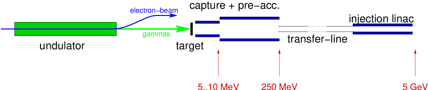
Figure 1: A schematic layout of the production of a longitudinal polarised positron beam in a linear collider as outlined in Ref. [1]. Marked by the arrows are the locations and their corresponding beam energies where a longitudinal polarimeter may be installed.

For the present study we select these three energy values i.e., 10, 250 and 5000 MeV, to represent those which eventually will be fixed by the final ILC design. To note is that even at 5000 MeV laboratory energy, the centre of mass energy of a positron hitting an electron in a fixed iron target of a Bhabha polarimeter is only $\sim$71.4 MeV. That is, far below the mass energy of the Z⁰ gauge boson. Thus it is here sufficient to describe the Bhabha scattering process of longitudinal polarised positrons and electrons in terms of the QED diagrams involving photon exchanges. The Bhabha process with longitudinal and transverse polarised beams is e.g. formulated in Ref. [9] for the case where only the QED processes contribute. In Ref. [10] the Bhabha scattering of longitudinal polarised beams is dealt with in terms of a semi-analytical approach realised by a Fortran program Zfitter which is valid at least up to $\sqrt{s}=350$ GeV, at or near the threshold energy of the $t\bar{t}$ quark$-$pair production. In this approach all the QED as well as the Z⁰ exchange processes and their interferences are included.

For the CM differential Bhabha scattering cross section at low energies, where the Z⁰ contribution and the running nature of the QED coupling constant can be ignored, we deduce from Ref. [10], in the absence of a transverse polarisation component, the following expression

$$\frac{d\sigma}{d\cos\theta}\ =\ \frac{\pi\alpha^{2}}{2s}\left[\lambda_{1}(1+\cos^{2}\theta)+2\lambda_{1}\frac{(1+\cos\theta)^{2}}{(1-\cos\theta)^{2}}+8\lambda_{3}\frac{1}{(1-\cos\theta)^{2}}-2\lambda_{1}\frac{(1+\cos\theta)^{2}}{(1-\cos\theta)}\right]\ .$$ (1)

Here $\theta$ is the polar centre of mass scattering angle of the positron and

$$\lambda_{1}\ =\ 1\ -\ \vec{P}_{+}\vec{P}_{-}\ \ \ \ {\rm{and}}\ \ \ \ \lambda_{3}\ =\ 1\ +\ \vec{P}_{+}\vec{P}_{-}\ ,$$

where $\vec{P}_{+}$ and $\vec{P}_{-}$ are respectively the longitudinal polarisation vector of the colliding positron beam and the electrons in the target which are defined in the range $0\leq|\vec{P}_{i}|\leq 1$. If one or both of the electron and positron beams are unpolarised, then one has $\lambda_{1}=\lambda_{3}=1$,

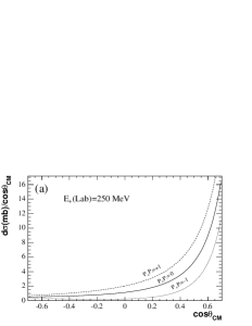
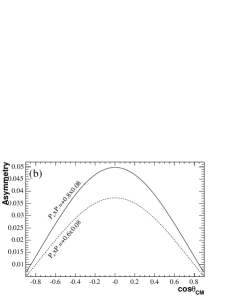
Figure 2: (a) The differential cross sections of the Bhabha scattering at 250 MeV beam energy as a function of $\cos\theta_{CM}$ for three longitudinal polarisation values which display the analysing power of a Bhabha polarimeter. (b) The Bhabha scattering asymmetry $A$ versus $\cos\theta_{CM}$. The continuous and dashed lines represent the polarisation values of $\vec{P}_{+}\vec{P}_{-}=+0.8\times$0.08 and +0.6$\times$0.08 respectively.

so that the Bhabha differential cross section is reduced to

$$\frac{d\sigma(P_{+}P_{-}=0)}{d\cos\theta}=\frac{\pi\alpha^{2}}{2s}\frac{(3+\cos^{2}\theta)^{2}}{(1-\cos\theta)^{2}}.$$ (2)

To illustrate the polarisation analysing power given by Eq. (1) we show in Fig. 2a the Bhabha scattering differential cross section at 250 MeV beam energy for two limits of the longitudinal polarisation states i.e., for $\vec{P}_{+}\vec{P}_{-}$ equal to +1 and $-$1 and for the zero polarisation case. As can be seen, there is a substantial difference between the magnitudes of the differential Bhabha scattering for these three polarisation states which can be utilised for the polarisation measurement. In practice however, the iron polarisation level cannot exceed the value of 0.08 and it is judged that the positron beam polarisation will not reach levels higher than $\sim$0.6.

The measurable asymmetry $A$, which is a function of $x~{}(\equiv\cos\theta_{CM})$, is given in the centre of mass system by

$$A\ =\ \frac{d\sigma/dx(\rightrightarrows)-d\sigma/dx(\leftrightarrows)}{d\sigma/dx(\rightrightarrows)+d\sigma/dx(\leftrightarrows)}\ =\ \frac{7-6x^{2}-x^{4}}{(3+x^{2})^{2}}\vec{P}_{+}\vec{P}_{-}\ \ \stackrel{{\scriptstyle\theta=\pi/2}}{{\overrightarrow{\hskip 42.67912pt}}}\ \frac{7}{9}\vec{P}_{+}\vec{P}_{-}$$ (3)

which is shown, as a function of $\cos\theta_{CM}$, in Fig. 2b for the combined polarisation values of $\vec{P}_{+}\vec{P}_{-}=+0.8\times 0.08$ and $+0.6\times 0.08$. Here we denote by $(\rightrightarrows)$ and $(\leftrightarrows)$ respectively the states where the positron beam polarisation is parallel and anti-parallel to the target electron polarisation direction. This asymmetry behaviour is identical to that one found for the Møller scattering (see e.g. Ref. [11]) where at $\cos\theta_{CM}=0$ reaches the maximum value of $(7/9)\times\vec{P}_{+}\vec{P}_{-}$. Assuming the beam polarisation to reach the high value of 0.8, then the resulting differential cross section are shown in Fig. 3 at 250 and 5000 MeV beam energy for three polarisation states.

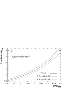
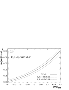
Figure 3: The differential Bhabha cross section in the centre of mass system as a function of $\cos\theta_{CM}$ at laboratory positron beam energy of (a) 250 and (b) 5000 MeV having three polarisation levels of $\pm$0.8 and zero while the iron target polarisation level is 0.08.

2.1 The features of a polarimeter setup

Two of the main elements of a Bhabha (or Møller) polarimeter consist of a magnetised iron, or iron alloy, target and a detector system for the identification and recording of the scattering process. In the present work we consider an iron target of a 10$\mu$m, a width which has been previously successfully applied to a Møller polarimeter [12], in order to reduce as much as possible secondary interactions and other background sources like the bremsstrahlung. The target, which is cooled down to $\sim$110 K, is placed in a magnetic field to reach the polarisation level of about 8$\%$ which is its maximum possible value due to the fact that only two out of the iron 26 electrons can be polarised. In a high magnetic field, of about four Tesla, it was shown that a target made out of thin iron foils, can be polarised out-of-plane in saturation [12, 13] i.e., parallel to the charged lepton beam direction. At moderate and low magnetic fields the polarisation direction is found to lie in the plane of the target face. In this case the target has to be tilted in the direction of the beam in order to increase the $|\vec{P}_{+}\vec{P}_{-}|$ value to achieve a sufficiently high polarisation analysing power. This tilt however increases the actual target thickness for example, from 10$\mu$m to 29.2$\mu$m, when the target is placed at 20⁰ with respect to the beam direction. Since the introduction of a high magnetic field of the order of $\sim$4 Tesla into the accelerating domain may be prohibited, we have taken for our Monte Carlo simulation study the less favourable target thickness of 30$\mu$m.

Here it should be noted that during the operation of a Bhabha polarimeter the iron target should not heat up and with it, reduce or completely loose, its polarisation. This heating problem, which depends among others factors on the beam current and its structure and on the measurement duration, can be kept under control even at relatively high currents of several tens of $\mu$A (see e.g. Ref. [11]). In any case, an online measurement of the relative iron foil polarisation during the polarimeter operation should be carried out for example with a laser beam making use of the polar Kerr effect [13].

Further we envisage that the Bhabha scattering outgoing charged leptons are steered into the polarimeter detector via a magnetic field which allows one to separate the electrons from the positrons and prevents the outgoing photons from hitting the detector. For the recording of the Bhabha events we foresee a pixel detector which covers a sizable part of the azimuthal angle region and an adequate polar angle range in the laboratory angular region which we here, in our feasibility study, set to be the one corresponding to the centre of mass cosine angle of $-$0.65 to +0.4. The setting of these limits at the corresponding laboratory angles can be realised for example by adjustable collimators similar to the ones applied previously to a Møller polarimeter [12] which selected the range of scattering angles and did cut off electrons at both smaller and larger angles. Furthermore, in that polarimeter setup, in front of the detector two slits were placed to define the actual acceptance of the polarimeter. However, as will be shown later, unlike the case of a Møller polarimeter, the need for an energy measurement of the outgoing electrons may be relaxed in a Bhabha polarimeter. The dimension of Bhabha polarimeter detector will have eventually to be determined by its distance from the target and the angular spread caused by the specific magnetic-optic system to be used. Finally the number of pixels and their size, is above all dictated by the need to keep the multiple-hit pixels to an insignificant number between the readout times of the detector.

3 Monte Carlo simulation

The features of Bhabha polarimeter using a fixed iron target of 30$\mu$m width operating with positron beams having the energies of 10, 250 and 5000 MeV were simulated via the GEANT4 Monte Carlo program [14, 15] which is currently void of spin effects. As a consequence our study on the Bhabha polarimeter sensitivity to the angular distribution of the scattering cross section and its strength, is carried out in the vicinity of zero polarisation. However judging from Fig. 2a where the Bhabha scattering dependence on $\cos\theta_{CM}$ at 250 MeV is shown for the two extreme polarisation cases of $P_{+}P_{-}=\pm 1$ and remembering that in practice $P_{-}=0.08$, the features of the polarimeter should essentially be independent of the positron polarisation level. In the simulations 200 Million positrons did hit the polarimeter target in each of the above selected beam energies and the outgoing positive and negative particles were recorded.

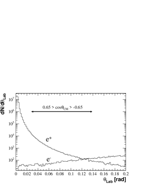
Figure 4: The laboratory $\theta_{Lab}$ angular distributions, in the range 0 to 0.2 rad, of the outgoing electrons and positrons as obtained from a GEANT4 Monte Carlo generated sample of a 250 MeV positron beam hitting an iron target of a 30$\mu$m thickness. The horizontal solid line marks the range corresponding to the CM cosine angle between $-$0.65 and +0.65.

It was found out that at 10 and 250 MeV essentially all the outgoing charged particles were electron and positrons. At the beam energy of 5000 MeV some charged final states hadrons were also observed. In Fig. 4 the laboratory $\theta_{Lab}$ angular distribution at 250 MeV beam energy is shown for the outgoing positrons and electrons. Within the range of $\theta_{Lab}$ of 0.1377 and 0.0293 rad, which corresponds in the CM to the region $-0.65\leq\cos\theta_{CM}\leq+0.65$, one observes that the ratio of positrons to electrons is about 19. This ratio and those found at 10 and 5000 MeV beam energies are listed in Table 1 where they are seen to lie in the range of $\sim$20 to $\sim$16. From the Monte Carlo studies follows that these large ratios, which in the absence of background should be equal to one, are mainly due to the contribution of the bremsstrahlung process which contains in its final state a positron. To eliminate this dominant background we further restrict our analysis to the detected outgoing electrons and show that these are sufficient to identify the Bhabha scattering process and to measure the beam polarisation.

Table 1: Monte Carlo results for the ratio of the outgoing positrons to the outgoing electrons, and the ratio between the background (BG) electrons to the total outgoing electrons emerging within the centre of mass symmetric polar angle range of $-0.65\leq\cos\theta_{CM}\leq+0.65$. The data are shown for the three positron beam laboratory energies of 10, 250 and 5000 MeV impinging on an iron target of 30$\mu$m effective width. The values given in the brackets refers to a target width of 10$\mu$m thickness.

Beam energy [MeV]	$\theta_{Lab}$ range [rad]	No. e+/No. e-	Fraction of BG e-
10	$0.5940\ -\ 0.1424$	19.9	$--$
250	$0.1377\ -\ 0.0293$	18.9	6.3$\%$  (2.0$\%$)
5000	$0.0310\ -\ 0.0066$	16.5	64$\%$  (22.5$)\%$

Next we turn to the relation between the laboratory energy of the outgoing electrons and their scattering angle $\theta_{Lab}$ which is given, in terms of $\cos\theta_{Lab}$, by

$$E_{Lab}\ =\ m_{e}\frac{\gamma+1+(\gamma-1)\cos^{2}\theta_{Lab}}{\gamma+1-(\gamma-1)\cos^{2}\theta_{Lab}}\ .$$ (4)

This relation is shown in Fig. 5a for a positron beam energy of 250 MeV. In Figs. 5b, 5c and 5d are shown the Monte Carlo generated scatter plots of the laboratory energy of the negative outgoing leptons versus

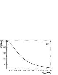
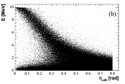
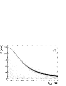
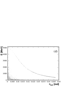
Figure 5: The Bhabha polarimeter response to the outgoing electrons laboratory energy on their scattering angle $\theta_{Lab}$ in the range corresponding to $\theta_{CM}=0$ to 2.55 rad. (a) The dependence as calculated from Eq. (4), at beam energy of 250 MeV. The scatter plots (b), (c) and (d) were obtained from GEANT4 Monte Carlo generated electrons samples produced at each energy by 200 Million positrons hitting a 30$\mu$m thick fixed iron target. The plots (b), (c), and (d) correspond respectively to 10, 250 and 5000 MeV beam energy.

their angle $\theta_{Lab}$ for respectively 10, 250 and 5000 MeV incident positron beam energy. Each scatter plot was produced by $200\times$$10^{6}$ positrons impinging on an iron target.

By comparing at 250 MeV the Monte Carlo results with the calculated distribution one univocally identifies the dense band, which is well separated from the background, as belonging to the Bhabha scattering process. This situation is also true for the 5000 MeV beam energy scatter plot shown in Fig. 5d where the background is lying even further away from the Bhabha signal. At 10 MeV beam energy however the isolation of the Bhabha scattering signal is severely hampered by the large background which is seen to merge with the signal at about $\theta_{Lab}\gtrsim 0.25$ rad. From the Monte Carlo studies the low energy background, seen in all the three energy scatter plots, stems mainly from Compton scattering and $e^{+}e^{-}$ pairs produced in the iron target by soft secondary photons the amount of which is seen to be approximately the same at 250 and 5000 MeV incoming beam energy. The higher energy background seen at small angles is coming from Bhabha scattering events where the outgoing electron suffered further on energy loss before emerging out of the target. As expected, the Bhabha scattering signal is smaller at 5000 MeV than at 250 MeV and as a consequence the signal to background ratio is also smaller as the beam energy increases. In view of all these observations it is safe to conclude that the option to place a Bhabha polarimeter in the region where the beam energy is 10 MeV or less is clearly disfavoured and should, if possible, be avoided. Both the 250 and 5000 MeV locations, which are a priori suitable for the installation of a Bhabha polarimeter, are further explored in the next subsection.

3.1 The Bhabha scattering signals and their background

As has been shown in Fig. 5c and 5d, the Bhabha scattering events are concentrated along a band lying in the laboratory energy versus $\theta_{Lab}$ plane which are well separated from a background which is seen to be mainly concentrated at low energies and at the $(E_{Lab},\theta_{Lab})=(0,0)$ corner. In the $\theta_{Lab}$ region chosen here for the polarisation analyses, which corresponds to the range $-0.65\leq\cos\theta_{CM}\leq+0.4$, this background amounts only to a about 5.2$\%$ in the 250 MeV case and to $\sim$57$\%$ in the 5000 MeV case, out of the total number of the outgoing electrons. Therefore if one insists on the 5000 MeV location for the polarisation measuements the amount of background should be reduced e.g. by introducing an appropriate combined energy$-$angle cut. This option will require however a more elaborated experimental setup, like the one chosen for the Møller polarimeter described in Ref. [12], which allows to measure simultaneously the individual outgoing electrons angle and energy and not just simply count them within a predetermined angular sector. Here it is worthwhile to note the the reduction of the target width to 10$\mu$m is still leaving the background at the relative high level of 22.5$\%$.

To reaffirm the origin of the events in the bands shown in Fig. 5c we proceeded to analyse the angular distribution of the outgoing negative particles seen at 250 MeV beam energy in the centre of mass system assuming all of them to be electrons emerging from an unperturbed Bhabha scattering process. In this case the transformation from the Lab angle to the CM angle is given by

$$\cos\theta_{CM}=\frac{2-(\gamma+1)\tan^{2}\theta_{Lab}}{2+(\gamma+1)\tan^{2}\theta_{Lab}}$$ (5)

where $\gamma=E_{Lab}^{beam}/m_{e}$. The angular distribution of the the Monte Carlo generated outgoing electrons in the CM system is shown in Fig. 6. The solid line in the figure represents the results of a fit of Eq. (1) to the Monte Carlo generated data where the factor $\pi\alpha^{2}/(2s)$ is represented by a free normalisation factor N and $\vec{P}_{+}\vec{P}_{-}$ is the second free parameter. The results of the fit, which was carried out over the $\cos\theta_{CM}$ range between $-$0.65 to +0.4,

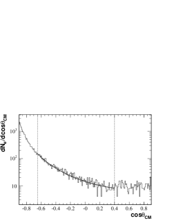
Figure 6: The centre of mass angular distribution of the outgoing electrons obtained from a GEANT4 Monte Carlo generated event sample of a 250 MeV positron beam hitting a 30$\mu$m thick fixed iron target. The solid line represents the fit results of Eq. (1) to the data in the $\cos\theta_{CM}$ range marked by the vertical dotted lines.

yielded

$$\vec{P}_{+}\vec{P}_{-}\ =\ 0.044\ \pm\ 0.126$$

which is consistent within errors with zero thus confirming the identity of the electron sample as arising predominantly from Bhabha scattering. An additional support for the Bhabha scattering origin of the electrons is given by the total number of Monte Carlo electrons emerging within the $\cos\theta_{CM}$ range of $-$0.65 to +0.4 which is consistent with that predicted by Eq. (1) when the low energy background given in Table 1 is subtracted. A similar fit procedure to the Monte Carlo data at 5000 MeV beam energy is prohibited due to the very large amount of background.

4 Measurement of the beam polarisation

For the measurement of the positron longitudinal polarisation we consider here a single$-$arm polarimeter, with a well defined angular acceptance, including a pixel detector for the electrons emerging from the Bhabha process. The polarisation measurement considered here rests on the two recorded numbers, $N_{+}$ and $N_{-}$, which represent respectively the total Bhabha scattering events detected when the beam$-$target polarisation directions are parallel i.e., $\vec{P}_{+}{\rightrightarrows}\vec{P}_{-}$, and when they are in opposite directions i.e., $\vec{P}_{+}{\leftrightarrows}\vec{P}_{-}$ . By counting $N_{+}$ and $N_{-}$ in the $x$ ($\equiv\cos\theta_{CM}$) range between $x_{min}$ and $x_{max}$ and using the Bhabha differential cross section $d\sigma/dx$ defined by Eq. (3), one obtains an experimental asymmetry $A_{exp}$ which is given by

$$A_{exp}=\frac{N_{+}-N_{-}}{N_{+}+N_{-}}=\frac{\int_{x_{min}}^{x_{max}}[d\sigma/dx(\rightrightarrows)-d\sigma/dx(\leftrightarrows)]dx}{\int_{x_{min}}^{x^{max}}[d\sigma/dx(\rightrightarrows)+d\sigma/dx(\leftrightarrows)]dx}=K(x_{max},x_{min})\vec{P}_{+}\vec{P}_{-}\ .$$ (6)

For the range $x_{min}=-0.65$ and $x_{max}=+0.4$ which was chosen here, the constant $K$ is equal to 0.696. From this follows that the positron beam longitudinal polarisation value is equal to

$$P_{+}\ =\ \frac{A_{exp}}{KP_{-}}\ ,$$ (7)

with the two independent error contributions

$$\Delta P_{+}=\frac{1}{KP_{-}}\Delta A_{exp}\ \ \ \rm{and}\ \ \ \Delta P_{+}=-\frac{A_{exp}}{KP_{-}^{2}}\Delta P_{-}\ .$$

Inasmuch that $P_{+}\neq 0$ the added in quadrature over all relative error squared of the measured beam polarisation is equal to

$$\left(\frac{\Delta P_{+}}{P_{+}}\right)^{2}=\left(\frac{\Delta A_{exp}}{A_{exp}}\right)^{2}+\left(\frac{\Delta P_{-}}{P_{-}}\right)^{2}~{},$$ (8)

where the statistical error squared of the measured asymmetry is

$$(\Delta A_{exp})^{2}\simeq 4\frac{N_{+}N_{-}}{N^{3}}=\frac{1-A_{exp}^{2}}{N}=\frac{1}{{\cal L}T\sigma_{x}}\left(1-(KP_{+}P_{-})^{2}\right)~{}.$$ (9)

Here $\sigma_{x}$ is the relevant cross section and $N=N_{+}+N_{-}$. The luminosity is equal to ${\cal{L}}=d\cdot\rho^{target}_{e}\cdot N^{beam}_{e}$ where $d$ is the thickness of the target, $\rho^{target}_{e}$ is the density of electrons in the target and $N^{beam}_{e}$ is the number of electrons hitting the target per second. Finally $T$ is the total measuring time. For convenience we further consider the case where the integrated luminosities for the parallel and anti-parallel polarisations of the positron beam and target electrons are the same i.e., ${\cal{L}}_{+}T_{+}$=${\cal{L}}_{-}T_{-}$. In this case one has

$$N=N_{+}+N_{-}={\cal L}\cdot T\cdot\sigma_{x}~{},$$

where $\sigma_{x}$ is the integrated cross section

$$\sigma_{x}=\int_{x_{min}}^{x_{max}}\frac{d\sigma}{dx}dx$$

which at 250 MeV beam energy is equal to $\sim$2.8 mb for $x_{min}=-0.65$ and $x_{max}=+0.4$. By using Eqs. (7) and (9) one can rewrite Eq. (8) as follows:

$$\left(\frac{\Delta P_{+}}{P_{+}}\right)^{2}=\frac{1}{{\cal L}T\sigma_{x}}\frac{1-(KP_{+}P_{-})^{2}}{(KP_{+}P_{-})^{2}}+\left(\frac{\Delta P_{-}}{P_{-}}\right)^{2}\ .$$ (10)

As long as $(KP_{+}P_{-})^{2}$  $\ll\ 1\$ one can simplify Eq. (10) to the form

$$\left(\frac{\Delta P_{+}}{P_{+}}\right)^{2}\simeq\frac{1}{{\cal L}T\sigma_{x}}\frac{1}{(KP_{+}P_{-})^{2}}+\left(\frac{\Delta P_{-}}{P_{-}}\right)^{2}.$$ (11)

Finally the time $t_{Int}$ needed to reach a desired relative beam polarisation precision of $\Delta P_{+}/P_{+}$ is given by

$$\frac{1}{t_{Int}}\simeq{\cal L}\left[\left(\frac{\Delta P_{+}}{P_{+}}\right)^{2}-\left(\frac{\Delta P_{-}}{P_{-}}\right)^{2}\right]\left(KP_{+}P_{-}\right)^{2}\sigma_{x},$$ (12)

which in turn determines the required number of scattering events, $N_{Int}={\cal L}\times t_{Int}\times\sigma_{x}$.

The high precision of $\Delta P_{-}/P_{-}=0.5\%$ has already been achieved for the polarisation of the magnetised iron target in a Møller polarimeter which operated in the JLAB [12] with an electron beam of a few $\mu$A in the energy range of 1 to 6 GeV. Thus it is expected from Eq. (11) that a low relative statistical error of $\Delta P_{+}/P_{+}$ $\simeq$ 0.5$\%$ may be achieved in a short time of a few seconds, with a 250 MeV positron beam of 0.1$\mu$A or even less. Eventually the over-all precision to be reached by a Bhabha polarimeter will thus depend mainly on the systematic uncertainties.

5 Summary and conclusions

The longitudinal polarisation measurement of a positron beam in a high energy linear collider is required near its production region to ascertain the polarisation existence and to allow the collider team to optimise its level by providing a fast polarisation measurement feedback. To satisfy these needs a fixed iron target polarimeter, the Bhabha polarimeter, is shown to constitute an attractive proposition. An iron target as thin as 10$\mu$m for a fixed target polarimeter has previously been constructed and it is expected to reduce to a minimum the various sources of background to the Bhabha scattering signal. Inasmuch that the collider design prohibits the presence of high magnetic fields of the order of four Tesla which can produce polarisation out-of plane, the iron polarisation will lie in the plane and the target must be tilted. Therefore we adopted here the more realistic case where the iron target is tilted and have shown that a reliable polarisation measurement can be achieved even when the target effective width increases to 30$\mu$m.

To suppress the major background due to bremsstrahlung events one should use for the Bhabha scattering identification and polarisation measurement only the outgoing electrons. These are sufficient to verify the Bhabha scattering identity and to supply the data for the polarisation measurement of the positron beam. Here one should note that a similar procedure is not applicable to the Møller polarimetry since both final state charged leptons are electrons.

The preferred location of a Bhabha polarimeter in a linear collide is found to be in the vicinity where the positron beam reaches the energy of 250 MeV. At this energy the final states are free of charged hadrons and at the same time the fraction of the non-Bhabha scattering electrons is still rather small and amounts to some 5.2$\%$ of the signal even at a target width of 30$\mu$m. In addition, at 250 MeV the measured laboratory angular sector of the outgoing electrons is in the range of several degrees and thus, from the engineering side, is relatively simple to implement. Finally the still large Bhabha scattering cross section guarantees a low background and a fast measurement feedback for the polarisation optimisation effort of the linear collider crew.

The option to install a Bhabha polarimeter in the region where the polarisation beam has an energy in the vicinity of 10 MeV is prohibited due to the fact that the background merges with the Bhabha scattering signal events. At 5000 MeV the Bhabha polarimetry is in principle possible however due to the presence of hadronic final states and in particular the relatively large fraction of the non-Bhabha scattering electrons it is a less favourable location for a Bhabha polarimetry than that at 250 MeV. On the other hand the construction of a more elaborated polarimeter may allow the removal of the high background at the 5000 MeV location by applying appropriate energy and angle cutoffs. The polarisation measurement duration at 5000 MeV is expected to be longer by a factor of $\sim$20 than that at 250 MeV but still short enough to provide a sufficiently fast feedback to the collider operating team.

Acknowledgements
We would like to thank H. Abramowicz, Y. Ben-Hammou, S. Kananov, K. Mönig, S. Riemann, T. Riemann and A. Stahl for many helpful discussions. Our thanks are also due to the DESY/Zeuthen particle research centre and its director U. Gensch, where part of the work reported here took place.

References

- [1] TESLA Technical Design Report, DESY-2001-011, March 2001.
- [2] GLC Project: Linear Collider for TeV Physics, KEK report 2003-7.
- [3] Luminosity, Energy and Polarization studies for the linear collider: comparing and for NLC and TESLA, SLAC-PUB-10353, physics/0403037.
- [4] G. Moortgat-Pick et al., Revealing fundamental interactions: the role of polarized positrons and electrons at the Linear Collider, CERN-PH-TH/2005-036, DCPT-04-100, IPPP-04-50, SLAC-PUB-11087, to be published in Physics Reports.
- [5] The SLD collaboration, Kenji Ahe et al., Phys. Rev. Lett. 84 (2000) 5945.
- [6] V.E. Balakin and A.A. Mikhailichenko, Budker Institute of Nuclear Physics, Preprint BINP 79-85 (1979).
- [7] G. Alexander et al., E166 Collaboration, Undulator-based production of polarized positrons: A proposal for the 50-GeV beam in the FFTB, SLAC-TN-04-018, LC-DET-2003-044.
- [8] See e.g., P. Schüler, The TESLA Compton polarimeter, Linear Collider Note, LC-DET-2001-047.
- [9] F.M. Renard, Basics of Electron Positron Collisions, (Edition Frontire) 1981, p.93.
- [10] D. Yu. Bardin et al., Comput. Phys. Commun. 133 (2001) 229.
- [11] See e.g., G. Alexander and I. Cohen, Nucl. Instr. and Meth. A 486 (2002) 552 and references therein.
- [12] See e.g., M. Hauger et al., Nucl. Instr. and Meth., A 462 (2001) 382.
- [13] L.V. de Bever et al., Nucl. Instr. and Meth. A 400 (1997) 379.
- [14] GEANT4 Collaboration, S. Agostinelli et al., Nucl. Instr. and Meth. A 506 (2003) 250.
- [15] GEANT4, Physics Reference Manual, available from http://cern.ch/geant4.