Deeply virtual and exclusive electroproduction of $\omega$ mesons

Abstract

The exclusive $\omega$ electroproduction off the proton was studied in a large kinematical domain above the nucleon resonance region and for the highest possible photon virtuality ($Q^{2}$) with the 5.75 GeV beam at CEBAF and the CLAS spectrometer. Cross sections were measured up to large values of the four-momentum transfer ($-t<2.7$ GeV²) to the proton. The contributions of the interference terms $\sigma_{TT}$ and $\sigma_{TL}$ to the cross sections, as well as an analysis of the $\omega$ spin density matrix, indicate that helicity is not conserved in this process. The $t$-channel $\pi^{0}$ exchange, or more generally the exchange of the associated Regge trajectory, seems to dominate the reaction $\gamma^{*}p\to\omega p$, even for $Q^{2}$ as large as 5 GeV². Contributions of handbag diagrams, related to Generalized Parton Distributions in the nucleon, are therefore difficult to extract for this process. Remarkably, the high-$t$ behaviour of the cross sections is nearly $Q^{2}$-independent, which may be interpreted as a coupling of the photon to a point-like object in this kinematical limit.

1 Introduction

The exclusive electroproduction of vector mesons is a powerful tool, on one hand to understand the hadronic properties of the virtual photon ($\gamma^{*}$) which is exchanged between the electron and the target nucleon Bau78 , and on the other hand to probe the quark-gluon content of the proton ($p$) Str94 ; Vdh97 ; Can02 . At moderate energies in the $\gamma^{*}p$ system, but large virtuality of the photon, quark-exchange mechanisms become significant in the vector meson production reactions $\gamma^{*}p\to p\rho$/$\omega$, thus shedding light on the quark structure of the nucleon.

The interaction of a real photon with nucleons is dominated by its hadronic component. The exchange in the $t$-channel of a few Regge trajectories permits a description of the energy dependence as well as the forward angular distribution of many, if not all, real-photon-induced reactions (see e.g. Ref. Don02 ). For instance, this approach reproduces the photoproduction of vector mesons from the CEBAF energy range to the HERA range (a few to 200 GeV) Lag00 . The exchange of the Pomeron (or its realization into two gluons) dominates at high energies, while the exchange of meson Regge trajectories ($\pi$, $\sigma$, $f_{2}$) takes over at low energies. At $\gamma p$ energies of a few GeV, $\omega$ photoproduction off a proton is dominated by $\pi^{0}$ exchange in the $t$-channel (fig. 1). The use of a saturating Regge trajectory Can02 is very successful in describing recent photoproduction data Bat03 at large angles (large momentum transfer $t$). This is a simple and economical way to parameterize hard scattering mechanisms. Extending these measurements to the virtual photon sector opens the way to tune the hadronic component of the exchanged photon, to explore to what extent $\pi^{0}$ exchange survives, and to observe hard scattering mechanisms with the help of a second hard scale, the virtuality $Q^{2}$ of the photon.

The study of such reactions in the Bjorken regime holds promise, through perturbative QCD, to access the so-called Generalized Parton Distributions (GPD) of the nucleon Ji97 ; Bel05 . These structure functions are a generalization of the parton distributions measured in the deep inelastic scattering experiments and their first moment links them to the elastic form factors of the nucleon. Their second moment gives access to the sum of the quark spin and the quark orbital angular momentum in the nucleon Ji97 . The process under study may be represented by the so-called handbag diagram (fig. 1). Its amplitude factorizes Col97 into a “hard” process where the virtual photon is absorbed by a quark and a “soft” one containing the new information on the nucleon, the GPD (which are functions of $x$ and $x^{\prime}$, the momentum fraction carried by the quark in the initial and final states, and of $t$, the squared four-momentum transfer between the initial and final protons). The factorization applies only to the transition, at small values of $-t$, between longitudinal photons ($L$) and helicity-0 mesons, which is dominant in the Bjorken regime. Because of the necessary gluon exchange to produce the meson in the hard process (see fig. 1), the dominance of the handbag contribution is expected to be reached at a higher $Q^{2}$ for meson production than for photon production (DVCS). Nevertheless, recent results on deeply virtual $\rho$ production show a qualitative agreement with calculations based on the handbag diagram Air00 ; Had04 . Vector meson production is an important complement to DVCS, since it singles out the quark helicity independent GPD $H$ and $E$ which enter Ji’s sum rule Ji97 and allows, in principle, for a flavor decomposition of these distributions (see e.g. Ref. Die03 ).

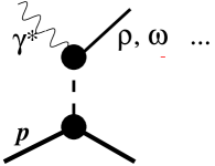
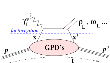
Figure 1: Schematic representations of the $t$-channel exchange (left) and of the handbag diagram (right) for exclusive vector meson electroproduction.

Apart from early, low statistics, muon production experiments at SLAC Bal74 ; Pap79 , the leptoproduction of $\omega$ mesons was measured at DESY Joo77 , for $0.3<Q^{2}<1.4$ GeV², $W<2.8$ GeV ($x_{B}<0.3$), and then at Cornell Cas81 , in a wider kinematical range ($0.7<Q^{2}<3$ GeV², $W<3.7$ GeV) but with larger integration bins. These two experiments yielded cross sections differing by a factor of about 2 wherever they overlap (around $Q^{2}\simeq$ 1 GeV²). The DESY experiment also provided the only analysis so far, in electroproduction, of the $\omega$ spin density matrix elements, averaged over the whole kinematical range. This analysis indicated that, in contrast with $\rho$ electroproduction, there is little increase in the ratio $R$ of longitudinal to transverse cross sections ($\sigma_{L}/\sigma_{T}$) when going from photoproduction to low $Q^{2}$ electroproduction. More recently, $\omega$ electroproduction was measured at ZEUS Bre00 , at high $Q^{2}$ and very low $x_{B}$, in a kinematical regime more sensitive to purely diffractive phenomena and to gluons in the nucleon. Finally, there is also unpublished data from HERMES Tyt01 .

The main goal of the present experiment was to reach the highest achievable $Q^{2}$ values in exclusive meson electroproduction in the valence quark region. In the specific case of the $\omega$ production, it is to test which of the two descriptions — with hadronic or quark degrees of freedom, more specifically $t$-channel Regge trajectory exchange or handbag diagram — applies in the considered kinematical domain (see fig. 2). For this purpose, the reduced cross sections $\sigma_{\gamma^{*}p\to\omega p}$ were measured in fine bins in $Q^{2}$ and $x_{B}$, as well as their distribution in $t$ and $\phi$ (defined below). In addition, parameters related to the $\omega$ spin density matrix were extracted from the analysis of the angular distribution of the $\omega$ decay products. If the vector meson is produced with the same helicity as the virtual photon, $s$-channel helicity conservation (SCHC) is said to hold. From our results, the relevance of SCHC and of natural parity exchange in the $t$-channel was explored in a model-independent way. These properties have been established empirically in the case of photo- and electroproduction of the $\rho$ meson (see e.g. Ref. Ros71 ), but may not be a general feature of all vector meson production channels.

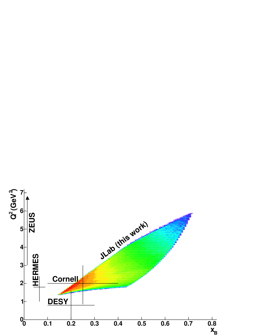
Figure 2: (Color online) Kinematical range covered by this and previous Joo77 ; Cas81 ; Bre00 ; Tyt01 $\omega$ electroproduction experiments. The lines are indicative of the total coverage in $Q^{2}$ and $x_{B}$ of previous experiments.

This paper is based on the thesis work of Ref. Mor03 , where additional details on the data analysis may be found.

2 Experimental procedure

We measured the process $ep\to ep\omega$, followed by the decay $\omega\to\pi^{+}\pi^{-}\pi^{0}$. The scattered electron and the recoil proton were detected, together with at least one charged pion from the $\omega$ decay. At a given beam energy $E$, this process is described by ten independent kinematical variables. In the absence of polarization in the $ep$ initial state, the observables are independent of the electron azimuthal angle in the laboratory. $Q^{2}$ and $x_{B}$ are chosen to describe the $\gamma^{*}p$ initial state. The scattered electron energy $E^{\prime}$ and, for ease of comparison with other data, the $\gamma^{*}p$ center-of-mass energy $W$ will be used as well. $t$ is the squared four-momentum transfer from the $\gamma^{*}$ to the $\omega$, and $\phi$ the angle between the electron ($ee^{\prime}\gamma^{*}$) and hadronic ($\gamma^{*}\omega p$) planes. Since $t$ is negative and has a kinematical upper bound $t_{0}(Q^{2},x_{B})$ corresponding to $\omega$ production in the direction of the $\gamma^{*}$, the variable $t^{\prime}=t_{0}-t$ will also be used. The $\omega$ decay is described in the so-called helicity frame, where the $\omega$ is at rest and the $z$-axis is given by the $\omega$ direction in the $\gamma^{*}p$ center-of-mass system. In this helicity frame, the normal to the decay plane is characterized by the angles $\theta_{N}$ and $\varphi_{N}$ (fig. 3). Finally the distribution of the three pions within the decay plane is described by two angles and a relative momentum. This latter distribution is known from the spin and parity of the $\omega$ meson Ste62 and is independent of the $\gamma^{*}p\to\omega p$ reaction mechanism. The purpose of the present study is to characterize as completely as possible the distributions of cross sections according to the six variables $Q^{2}$, $x_{B}$, $t$, $\phi$, $\cos\theta_{N}$ and $\varphi_{N}$.

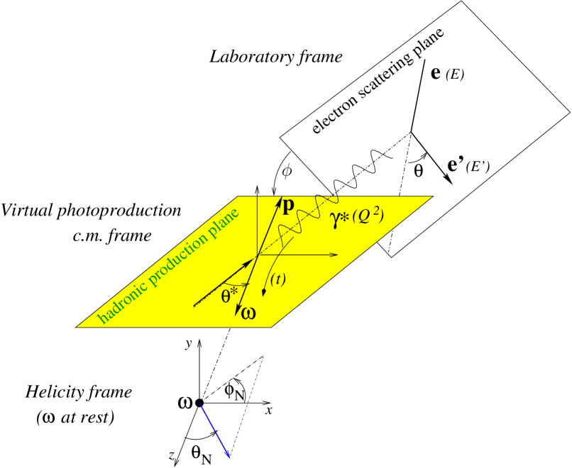
Figure 3: (Color online) Reference frames and relevant variables used for the description of the reaction $ep\to ep\omega$, followed by $\omega\to\pi^{+}\pi^{-}\pi^{0}$.

2.1 The experiment

The experiment was performed at the Thomas Jefferson National Accelerator Facility (JLab). The CEBAF 5.754 GeV electron beam was directed at a 5-cm long liquid-hydrogen target. The average beam intensity was 7 nA, resulting in an effective integrated luminosity of 28.5 fb^-1 for the data taking period (October 2001 to January 2002). The target was positioned at the center of the CLAS spectrometer. This spectrometer uses a toroidal magnetic field generated by six superconducting coils for the determination of particle momenta. The field integral varied approximately from 2.2 to 0.5 Tm, in average over charges and momenta of different particles, for scattered angles between 14^∘ and 90^∘. All the spectrometer components are arranged in six identical sectors. Charged particle trajectories were detected in three successive packages of drift chambers (DC), the first one before the region of magnetic field (R1), the second one inside this region (R2), and the third one after (R3). Threshold Čerenkov counters (CC) were used to discriminate pions from electrons. Scintillators (SC) allowed for a precise determination of the particle time-of-flight. Finally, a segmented electromagnetic calorimeter (EC) provided a measure of the electron energy. This geometry and the event topology are illustrated in fig. 4. A detailed description of the CLAS spectrometer and of its performance is given in Ref. CLAS .

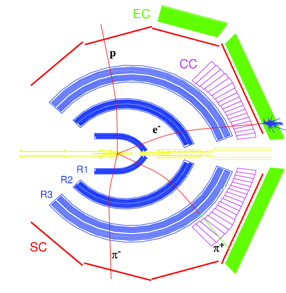
Figure 4: (Color online) Schematic view of the CLAS spectrometer components (see text for description) and of typical particle tracks, viewed in projection. The torus coils are not shown.

The data acquisition was triggered by a coincidence CC$\cdot$EC corresponding to a minimal scattered electron energy of about 0.575 GeV. The trigger rate was 1.5 kHz, with a data acquisition dead time of 6%. A total of $1.25\times 10^{9}$ events was recorded.

2.2 Particle identification

After calibration of all spectrometer subsystems, tracks were reconstructed from the DC information. The identification of particles associated with each track proceeded differently for electrons and hadrons.

Electrons were identified from the correlation between momentum (from DC) and energy (from EC). In addition pions were rejected from the electron sample by a cut in the CC amplitude and imposing a condition on the energy sharing between EC components compatible with the depth profile of an electromagnetic shower. Geometrical fiducial cuts ensured that the track was inside a high efficiency region for both CC and EC. The efficiencies of the electron identification cuts ($\eta_{CC}$ and $\eta_{EC}$) depended on the electron momentum and angle (or on $Q^{2}$ and $x_{B}$). $\eta_{EC}$ was calculated from data samples using very selective CC cuts in order to unambiguously select electrons. $\eta_{CC}$ was extracted from an extrapolation of the CC amplitude Poisson distribution into the low amplitude region. These efficiencies varied respectively between 0.92 and 0.99 (CC), and 0.86 to 0.96 (EC). At low electron energies, a small contamination of pions remained, which did not however satisfy the $\omega$ selection criteria to be described below.

The relation between momentum (from DC) and velocity (from path length in DC and time-of-flight in SC) allowed for a clean identification of protons ($p$) and pions ($\pi^{+}$ and $\pi^{-}$). However, for momenta larger than 2 GeV/$c$, ambiguities arose between $p$ and $\pi^{+}$ identification, which led us to the discarding of events corresponding to $t<-2.7$ GeV². Fiducial cuts were applied to hadrons as well. The efficiency for the hadron selection cuts was accounted for in the acceptance calculation described in sect. 2.4.

2.3 Event selection and background subtraction

Two configurations of events were studied, with one or two detected charged pions: $ep\to ep\pi^{+}X$ and $ep\to ep\pi^{+}\pi^{-}X$. The former benefits from a larger acceptance and is adequate to determine cross sections, while the latter is necessary to measure in addition the distribution of the $\omega$ decay plane orientation and deduce from it the $\omega$ spin density matrix. The final selection of events included cuts in $W$ and $E^{\prime}$: $W>1.8$ GeV to eliminate the threshold region sensitive to resonance production Bur02 and $E^{\prime}>0.8$ GeV to minimize radiative corrections and residual pion contamination in the electron tracks. The first configuration was selected requiring a missing mass $M_{X}$ larger than 0.316 GeV to eliminate two pion production channels ($M_{X}^{2}>0.1$ GeV² on the vertical axis of fig. 5). This cut was chosen slightly above the two pion mass in order to minimize background. The corresponding losses in $ep\to ep\omega$ events were very small and accounted for in the acceptance calculation to be discussed below. Events corresponding to the $\omega$ production appear as a clear peak in the $ep\to epX$ missing mass spectrum (fig. 6). The width of this peak ($\sigma\simeq 16$ MeV) is mostly due to the experimental resolution.

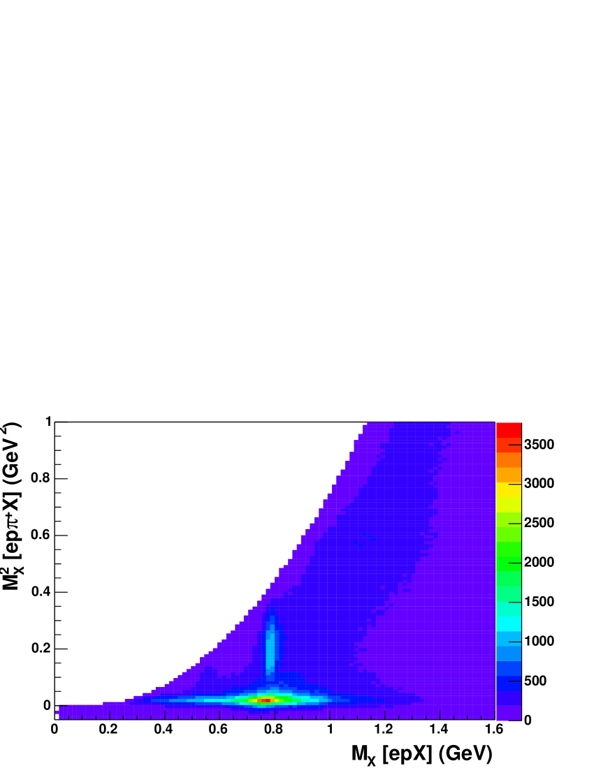
Figure 5: (Color online) Identification of the $\omega$ channel in the case of the detection of one charged pion: $M_{X}^{2}[ep\pi^{+}X]$ vs $M_{X}[epX]$. Events corresponding to $\rho$ (horizontal locus) and other two-pion production channels are clearly separated from those corresponding to $\omega$ production (vertical locus).

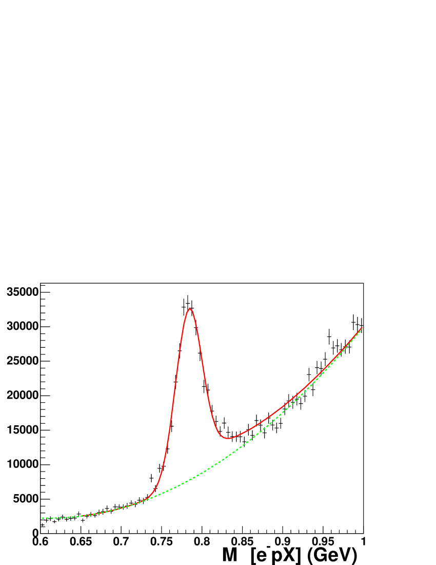
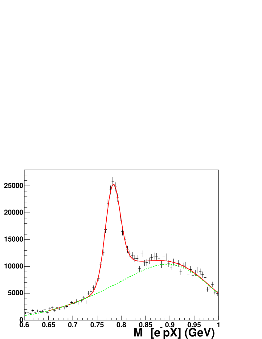
Figure 6: (Color online) Missing mass $M_{X}[epX]$ distributions for the $ep\to ep\pi^{+}X$ event configuration, for two ($Q^{2},x_{B}$) bins, after selection cuts and event weighting discussed in the text. Left : 2.2 GeV² $\leq Q^{2}\leq$ 2.5 GeV² and 0.34 $\leq x_{B}\leq$ 0.40. Right : 3.1 GeV² $\leq Q^{2}\leq$ 3.6 GeV² and 0.52 $\leq x_{B}\leq$ 0.58 (at the edge of kinematical acceptance). The two lines indicate the subtracted background (green) and the fitted distribution ($\omega$ peak + background in red).

After proper weighting of each event with the acceptance calculated as indicated in sect. 2.4, a background subtraction was performed for each of 34 bins ($Q^{2},x_{B}$) and, for differential cross sections, for each bin in $t$ or $\phi$. The background was determined by a fit to the acceptance-weighted distributions with a second-order polynomial and a peak shape as modeled by simulations (a skewed gaussian shape taking into account the experimental resolution and radiative tail). At the smallest values of $W$, the fitted background shape was modified to account for kinematical acceptance cuts. The acceptance-weighted numbers of $ep\to ep\omega$ events were computed using the sum of weighted counts in the $M_{X}[epX]$ distributions for $.72<M_{X}<.85$ GeV, diminished by the fitted background integral in the same interval.

Likewise, events from the second configuration ($ep\to ep\pi^{+}\pi^{-}X$) were selected with cuts in missing masses:
$M_{X}[ep\pi^{+}X]$ and $M_{X}[ep\pi^{-}X]>0.316$ GeV, $0.01\ \hbox{GeV}^{2}\leq M_{X}^{2}[ep\pi^{+}\pi^{-}X]\leq 0.045\ \hbox{GeV}^{2}$ (fig. 7). The resulting
$M_{X}[epX]$ spectrum after these cuts is illustrated in fig. 8. The background subtraction in the spectrum of weighted events proceeded in the same way for each of 64 ($Q^{2}$, $x_{B}$, $\cos\theta_{N}$) bins or for each of 64 ($Q^{2}$, $x_{B}$, $\varphi_{N}$) bins in order to analyze the $\omega$ decay distribution (see sect. 4).

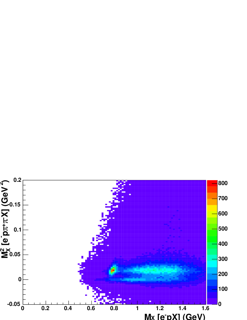
Figure 7: (Color online) Identification of the $\omega$ channel in the case of the detection of two charged pions: $M_{X}^{2}[ep\pi^{+}\pi^{-}X]$ vs $M_{X}[epX]$ for $M_{X}^{2}[ep\pi^{\pm}X]\geq$ 0.1 GeV². The spot at ( 0.78, 0.02) corresponds to the $\omega$.

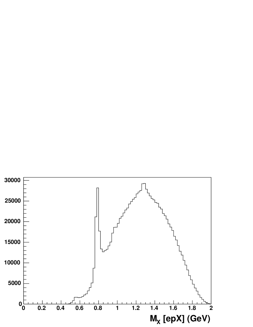
Figure 8: Unweighted $M_{X}[epX]$ spectrum for all $ep\to ep\pi^{+}\pi^{-}X$ events after selection cuts discussed in the text.

2.4 Acceptance calculation

The tracks reconstruction and the event selection were simulated using a GEANT-based Monte Carlo (MC) simulation of the CLAS spectrometer. We used an event generator tuned to reproduce photoproduction and low $Q^{2}$ data in the resonance region and extrapolated into our kinematical domain genev . The acceptance was defined in each elementary bin in all relevant variables as the ratio of accepted to generated MC events. At the limit of small six-dimensional bins, it is independent of the model used to generate the MC events. The MC simulation included a tuning of the DC and SC time resolutions to reproduce the observed widths of the hadron particle identification spectra and of the missing mass spectra, so that the efficiency of the corresponding cuts described above could be correctly determined.

For the extraction of cross sections from the $ep\to ep\pi^{+}X$ configuration, acceptance calculations were performed in 1837 four-dimensional bins ($Q^{2}$, $x_{B}$, $t$ and $\phi$) with two different assumptions about the event distribution in $\cos\theta_{N}$ and $\varphi_{N}$. The two different MC calculations were used for an estimate of the corresponding systematic uncertainties (see sect. 3.1). For the analysis of the decay plane distribution $\mathcal{W}(\cos\theta_{N},\varphi_{N},\phi)$ from the $ep\to ep\pi^{+}\pi^{-}X$ configuration, the acceptance calculation was performed in 3575 six-dimensional bins ($Q^{2}$, $x_{B}$, $t$, $\phi$, $\cos\theta_{N}$ and $\varphi_{N}$). The binning is defined in table 1 and the numbers above correspond to kinematically allowed bins that have significant statistics.

The calculated acceptances are, on average, of the order of 2% and 0.2% respectively for the two event configurations of interest. They vary smoothly for all variables except $\phi$, where oscillations, due to the dead zones in the CLAS sectors, reproduce the physical distributions of events (fig. 9). Each event was then weighted with the inverse of the corresponding acceptance. Events belonging to bins with either very large or poorly determined weights were discarded (for the $ep\to ep\pi^{+}X$ configuration, acceptance smaller than 0.25% or associated MC statistical uncertainty larger than 35%). The corresponding losses (a few percent) were quantified through the MC efficiency $\eta_{MC}$ by applying these cuts to MC events and computing the ratio of weighted accepted MC events to generated events. No attempt was made to calculate the acceptance for the non-resonant three-pion background, so that the background shape in fig. 6 differs from the physical distribution $d\sigma/dM_{X}$ when $M_{X}$ differs from the $\omega$ mass.

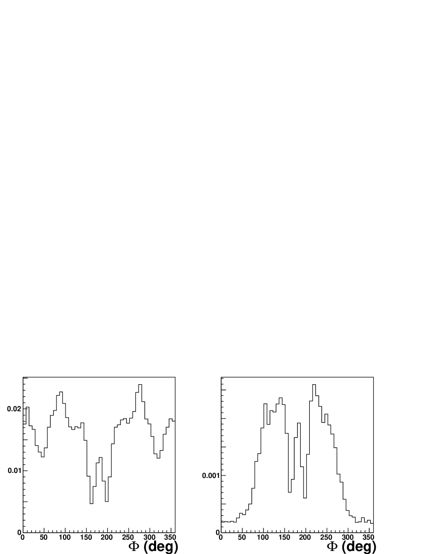
Figure 9: $\phi$ dependence of calculated acceptance, integrated over other kinematical variables, for the one and two detected pion configurations: $ep\to ep\pi^{+}X$ (left), $ep\to ep\pi^{+}\pi^{-}X$ (right).

2.5 Radiative corrections

Radiative corrections were calculated following Ref. Mo69 . They were dealt with in two separate steps. The MC acceptance calculation presented above took into account radiation losses due to the emission of hard photons, through the application of the cut $M_{X}[epX]<0.85$ GeV. Corrections due to soft photons, and especially the virtual processes arising from vacuum polarization and vertex correction, were determined separately for each bin in ($Q^{2}$, $x_{B}$, $\phi$). The same event generator employed for the computation of the acceptance was used, with radiative effects turned on and off, thus defining a corrective factor $F_{rad}$. The $t$-dependence of $F_{rad}$ is smaller than all uncertainties discussed in sect. 3.1 and was neglected.

3 Cross sections for $\gamma^{*}p\to\omega p$

The total reduced cross sections were extracted from the data through :

$$\sigma_{\gamma^{*}p\rightarrow\omega p}(Q^{2},x_{B},E) = \frac{1}{\Gamma_{V}(Q^{2},x_{B},E)}\times\frac{n_{w}(Q^{2},x_{B})}{B\mathcal{L}_{int}\Delta Q^{2}\cdot\Delta x_{B}}$$ (1)

$$\times\frac{F_{rad}}{\eta_{CC}\ \eta_{EC}\ \eta_{MC}}\ .$$

The Hand convention Han63 was used for the definition of the virtual transverse photon flux $\Gamma_{V}$, which includes here a Jacobian in order to express the cross sections in the chosen kinematical variables :

$$\Gamma_{V}(Q^{2},x_{B},E)=\frac{\alpha}{8\pi}\frac{Q^{2}}{M_{p}^{2}E^{2}}\frac{1-x_{B}}{x_{B}^{3}}\frac{1}{1-\varepsilon},$$ (2)

with the virtual photon polarization parameter being defined as :

$$\varepsilon=\frac{1}{1+2\frac{Q^{2}+(E-E^{\prime})^{2}}{4EE^{\prime}-Q^{2}}}\ .$$ (3)

In eq. (1), $n_{w}(Q^{2},x_{B})$ is the acceptance-weighted number of $ep\to ep\omega$ events after background subtraction. The branching ratio of the $\omega$ decay into three pions is $B=0.891$ PDG04 . The integrated effective lumimosity $\mathcal{L}_{int}$ includes the data acquisition dead time correction. $\Delta Q^{2}$ and $\Delta x_{B}$ are the corresponding bin widths; for bins not completely filled (because of $W$ or $E^{\prime}$ cuts on the electron, or of detection acceptance), the phase space $\Delta Q^{2}\cdot\Delta x_{B}$ includes a surface correction and the $Q^{2}$ and $x_{B}$ central values are modified accordingly. The radiative correction factor and the various efficiencies not included in the MC calculation were discussed in previous sections.

Differential cross sections in $t$ or $\phi$ were extracted in a similar manner. Cross section data and corresponding MC data for the acceptance calculation were binned according to table 1.

Table 1: Definition of binning for cross section (1) and $\omega$ polarization (2) data. N refers to the number of bins in the specified range for each variable.

Variable	Range(1)	N(1)	Range(2)	N(2)
$Q^{2}$ (GeV2)	1.6 - 3.1	5	1.7 - 4.1	4
	3.1 - 5.1	4	4.1 - 5.2	1
$x_{B}$	0.16 - 0.64	8	0.18 - 0.62	4
$-t$ (GeV2)	0.1 - 1.9	6	0.1 - 2.1	4
	1.9 - 2.7	1	2.1 - 2.7	1
$\phi$ (rd)	0 - 2$\pi$	9	0 - 2$\pi$	6/9/12
$\cos\theta_{N}$	-	-	$-1$ - 1	8
$\varphi_{N}$ (rd)	-	-	0 - 2$\pi$	8

3.1 Systematic uncertainties

Systematic uncertainties in the cross section measurements arise from the determination of the CLAS acceptance, of electron detection efficiencies, of the luminosity, and from the background subtraction. They are listed in table 2 and discussed hereafter.

Errors in the acceptance calculation may be due to inhomogeneity in the detectors response, such as faulty channels in DC or SC, to possible deviations between experimental and simulated resolutions in spectra where cuts were applied, to the input of the event generator (both in cross section and in decay distribution $\mathcal{W}_{gen}$), to radiative corrections and finally to the event weighting procedure. The most significant of these uncertainties (8%) was quantified by performing a separate complete MC simulation varying inputs for the parameters describing the decay distribution $\mathcal{W}_{gen}$.

Systematic uncertainties on the electron detection efficiencies were estimated with experimental data, by varying the electron selection cuts or the extrapolated CC amplitude distribution (see sect. 2.2).

Systematic background subtraction uncertainties were estimated by varying the assumed background functional shapes. In particular, the background curvature under the $\omega$ peak was varied between extreme values compatible with an equally good fit to the distributions in fig. 6. For bins corresponding to low values of $W$, the acceptance cut to the right of the $M_{X}[epX]$ peak induced an additional uncertainty.

Finally, overall normalization uncertainties were due to the knowledge of target thickness (2%) and density (1%) and of beam integrated charge (2%).

Errors contributing point-to-point and to the overall normalization are separately added in quadrature in table 2. For $t$ or $\phi$ distributions, the same uncertainties apply, but may contribute to the overall normalization uncertainty instead of point-to-point. For example, the shape of the $M_{X}[epX]$ distributions depends mostly on $Q^{2}$ and $x_{B}$, not on $t$ and $\phi$; the background subtraction uncertainties are then considered as a normalization uncertainty for the $d\sigma/dt$ and $d\sigma/d\phi$ distributions. The uncertainties on $\eta_{MC}$ are largest for $t$ and $\phi$ bins with the smallest acceptance (lowest and highest $t$ values, as well as $\phi\simeq 180^{\circ}$).

Table 2: Point-to-point and normalization systematic uncertainties, for integrated and differential cross sections.

Source of uncertainty	$\sigma$	$d\sigma/dt$	$d\sigma/d\phi$
CLAS acceptance
- inhomogeneities	6%	6%	6%
- resolutions	2%	2%	-
- $\sigma_{gen}(Q^{2},x_{B},t)$	5%	5%	-
- $\mathcal{W}_{gen}(\cos\theta_{N},\varphi_{N},\phi)$	8%	8%	-
- radiative corrections	4%	-	2%
- binning	5%	5%	-
- $\eta_{MC}$	4%	2-7%	2-20%
Electron detection
- $\eta_{CC}$	1.5%	-	-
- $\eta_{EC}$	2%	-	-
Background subtraction	7-11%	-	-
Point-to-point	16-18%	13-14%	7-21%
Normalization	3%	9-12%	14-16%

3.2 Integrated reduced cross sections

Results for $\sigma_{\gamma^{*}p\to\omega p}(Q^{2},x_{B})$ are given in table 3 and fig. 10. For the purpose of comparison with previous data, fig. 11 shows cross sections as a function of $Q^{2}$ for fixed, approximately constant, values of $W$. When comparing different data sets, note that $\sigma=\sigma_{T}+\varepsilon\sigma_{L}$ depends on the beam energy through $\varepsilon$. However, as will be shown, it is likely that the difference of longitudinal contributions between two different beam energies $(\varepsilon_{2}-\varepsilon_{1})\sigma_{L}$ is much smaller than the total cross section $\sigma$. In addition, the range of integration in $t$ is different for all experiments, larger in this work, but most of the total cross section comes from small $-t$ values. A direct comparison of the cross sections is then meaningful.

Table 3: Cross sections $\sigma=\sigma_{T}+\varepsilon\sigma_{L}$ and interference terms $\sigma_{TT}$ and $\sigma_{TL}$ for the reaction $\gamma^{*}p\to\omega p$, integrated over $-2.7\ \hbox{GeV}^{2}<t<t_{0}$. Slope $b$ of $d\sigma/dt$ for $-1.5\ \hbox{GeV}^{2}<t<t_{0}$. Quoted uncertainties are obtained from the addition in quadrature of statistical uncertainties and of point-to-point systematic uncertainties as discussed in sect. 3.1.

$x_{B}$	$Q^{2}$	$W$	$\varepsilon$	$t_{0}$	$\sigma\pm\Delta\sigma$	$\sigma_{TT}\pm\Delta\sigma_{TT}$	$\sigma_{TL}\pm\Delta\sigma_{TL}$	$b\pm db$
	(GeV2)	(GeV)		(GeV2)	(nb)	(nb)	(nb)	(GeV-2)
0.203	1.725	2.77	0.37	-0.09	536 $\pm$ 96	60 $\pm$ 87	2 $\pm$ 30	2.44 $\pm$ 0.18
0.250	1.752	2.48	0.59	-0.15	661 $\pm$ 118	156 $\pm$ 61	-35 $\pm$ 24	1.93 $\pm$ 0.16
0.252	2.042	2.63	0.43	-0.14	421 $\pm$ 75	104 $\pm$ 47	-18 $\pm$ 18	2.28 $\pm$ 0.16
0.265	2.320	2.70	0.32	-0.14	344 $\pm$ 62	58 $\pm$ 74	-14 $\pm$ 26	1.88 $\pm$ 0.17
0.308	1.785	2.21	0.72	-0.25	1139 $\pm$ 205	310 $\pm$ 122	-175 $\pm$ 60	1.23 $\pm$ 0.17
0.310	2.050	2.33	0.63	-0.23	551 $\pm$ 98	121 $\pm$ 42	-66 $\pm$ 20	1.90 $\pm$ 0.16
0.310	2.350	2.47	0.50	-0.21	395 $\pm$ 71	103 $\pm$ 41	-49 $\pm$ 17	2.03 $\pm$ 0.16
0.313	2.639	2.58	0.37	-0.20	287 $\pm$ 52	111 $\pm$ 48	-9 $\pm$ 18	1.90 $\pm$ 0.17
0.327	2.914	2.62	0.28	-0.22	226 $\pm$ 43	138 $\pm$ 84	-46 $\pm$ 27	1.87 $\pm$ 0.23
0.370	2.050	2.09	0.74	-0.37	1002 $\pm$ 180	91 $\pm$ 75	-25 $\pm$ 39	0.97 $\pm$ 0.17
0.370	2.350	2.21	0.65	-0.34	581 $\pm$ 104	150 $\pm$ 48	-36 $\pm$ 23	1.35 $\pm$ 0.17
0.370	2.650	2.32	0.55	-0.31	380 $\pm$ 68	85 $\pm$ 40	-33 $\pm$ 17	1.62 $\pm$ 0.17
0.370	2.950	2.43	0.43	-0.30	273 $\pm$ 49	95 $\pm$ 42	-44 $\pm$ 17	1.93 $\pm$ 0.18
0.378	3.295	2.51	0.31	-0.30	230 $\pm$ 42	17 $\pm$ 55	-27 $\pm$ 19	1.46 $\pm$ 0.18
0.429	2.055	1.90	0.81	-0.59	2203 $\pm$ 348	54 $\pm$ 158	143 $\pm$ 85	1.03 $\pm$ 0.25
0.430	2.350	2.00	0.74	-0.53	1013 $\pm$ 182	181 $\pm$ 82	-102 $\pm$ 43	0.78 $\pm$ 0.22
0.430	2.650	2.10	0.67	-0.49	626 $\pm$ 113	90 $\pm$ 63	-41 $\pm$ 32	0.81 $\pm$ 0.22
0.430	2.950	2.19	0.58	-0.46	427 $\pm$ 78	56 $\pm$ 48	-24 $\pm$ 23	0.92 $\pm$ 0.23
0.430	3.350	2.31	0.45	-0.43	265 $\pm$ 48	105 $\pm$ 37	-12 $\pm$ 15	1.34 $\pm$ 0.23
0.436	3.807	2.41	0.30	-0.42	191 $\pm$ 35	128 $\pm$ 60	-54 $\pm$ 21	1.47 $\pm$ 0.24
0.481	2.371	1.85	0.79	-0.79	1660 $\pm$ 265	-34 $\pm$ 173	241 $\pm$ 97	0.92 $\pm$ 0.50
0.490	2.651	1.91	0.74	-0.75	1113 $\pm$ 177	291 $\pm$ 109	15 $\pm$ 62	0.68 $\pm$ 0.37
0.490	2.950	1.99	0.68	-0.69	644 $\pm$ 116	174 $\pm$ 69	-154 $\pm$ 35	0.23 $\pm$ 0.34
0.490	3.350	2.09	0.58	-0.64	397 $\pm$ 72	84 $\pm$ 49	-49 $\pm$ 24	1.39 $\pm$ 0.25
0.490	3.850	2.21	0.43	-0.60	272 $\pm$ 50	72 $\pm$ 46	5 $\pm$ 20	1.41 $\pm$ 0.26
0.494	4.307	2.30	0.29	-0.58	187 $\pm$ 37	169 $\pm$ 79	-14 $\pm$ 27	0.78 $\pm$ 0.32
0.538	2.968	1.85	0.73	-0.99	894 $\pm$ 148	111 $\pm$ 148	8 $\pm$ 69	$-$
0.549	3.357	1.91	0.66	-0.96	514 $\pm$ 84	83 $\pm$ 67	-12 $\pm$ 31	$-$
0.550	3.850	2.01	0.55	-0.88	327 $\pm$ 59	95 $\pm$ 54	-52 $\pm$ 26	0.65 $\pm$ 0.49
0.550	4.350	2.11	0.41	-0.83	258 $\pm$ 48	29 $\pm$ 62	-13 $\pm$ 27	0.90 $\pm$ 0.43
0.557	4.765	2.16	0.31	-0.83	222 $\pm$ 44	-42 $\pm$ 121	55 $\pm$ 51	1.36 $\pm$ 0.67
0.601	3.882	1.86	0.61	-1.26	292 $\pm$ 57	91 $\pm$ 89	74 $\pm$ 50	$-$
0.610	4.352	1.91	0.52	-1.24	221 $\pm$ 43	75 $\pm$ 54	-53 $\pm$ 23	$-$
0.610	4.850	2.00	0.40	-1.16	150 $\pm$ 26	-110 $\pm$ 48	39 $\pm$ 20	$-$

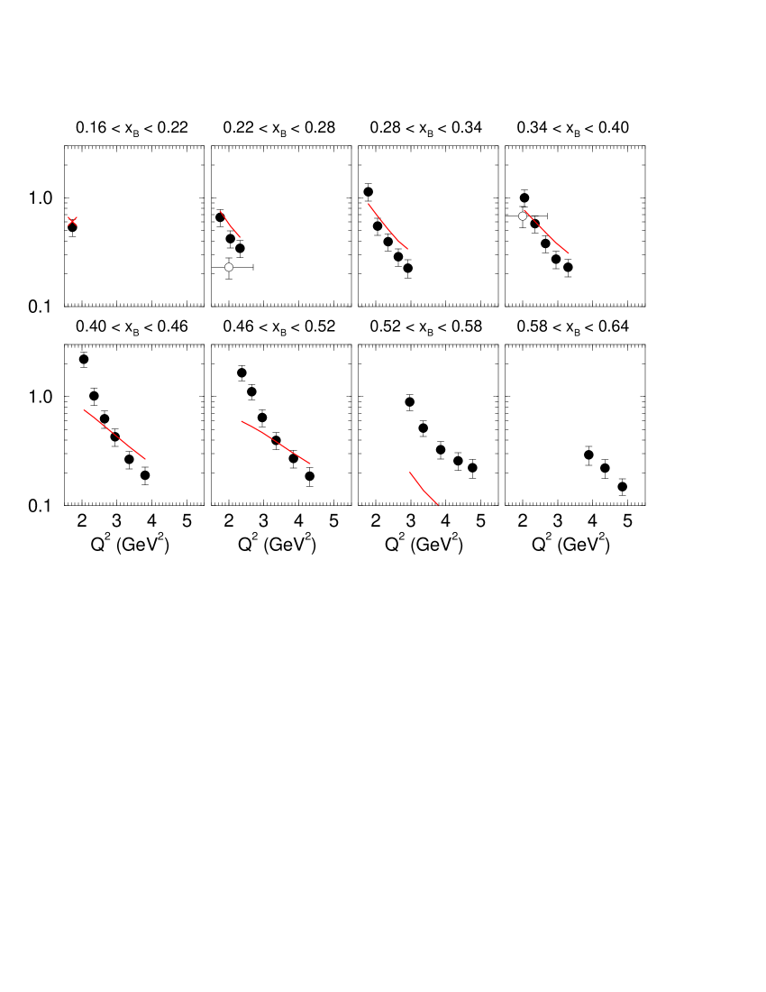
Figure 10: (Color online) Reduced cross sections $\gamma^{*}p\rightarrow\omega p$ as a function of $Q^{2}$ for differents bins in $x_{B}$, in units of $\mu$b. Full circles: this work; open circles: Ref. Cas81 . The red cross and curves correspond to the JML model Lag04 discussed in sect. 5.

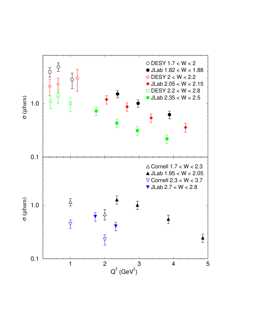
Figure 11: (Color online) Total cross sections for the reaction $\gamma^{*}p\to\omega p$, as a function of $Q^{2}$ and at fixed $W$ : this work in full symbols, DESY Joo77 (top) and Cornell Cas81 (bottom) in open symbols. Each symbol (or color) corresponds to a given central value of $W$ (GeV). Note the range of integration in $W$ for each data set.

There is no direct overlap between the present data and the DESY data Joo77 , but they seem to be compatible with a common trend. The Cornell data Cas81 are roughly a factor 2 lower than ours. Where they overlap, the Cornell data are also a factor 2 lower than the DESY data. We can only make the following conjectures as to the origin of this discrepancy: the Cornell results do not appear to have been corrected for internal virtual radiative effects (about 15%); their overall systematic uncertainty in absolute cross sections is 25%; their acceptance calculation has a model dependence which was not quantified and in particular the decay distribution, given in eq. (4) below, was assumed flat; finally, the estimate of average values of kinematical variables $\langle Q^{2}\rangle$ and $\langle W\rangle$ may be an additional source of uncertainty since the corresponding bins are at least 5 times larger than in the present work.

3.3 $t$ dependence of cross sections

Four of the 34 distributions of differential cross sections are illustrated in fig. 12.

Figure 12: $d\sigma/dt$ for the reaction $\gamma^{*}p\to\omega p$, at $W$ $\simeq$ 2.45 GeV for different bins in $Q^{2}$ : our data and the JML model (discussed in sect. 5) with $F_{\pi\omega\gamma}$ given by eq. (14) (full lines) and without the $t$-dependence in this equation (dashed lines).

The general features of these distributions are of a diffractive type ($d\sigma/dt\propto e^{bt}$) at small values of $-t$. The values of the slope $b$, as determined from a fit of the distributions in the interval -1.5 GeV${}^{2}<t<t_{0}$, are between 0.5 and 2.5 GeV^-2 and are compiled in table 3. They are also plotted as a function of the formation length (distance of fluctuation of the virtual photon in a real meson) Bau78 :

$$c\Delta\tau=\frac{1}{\sqrt{\nu^{2}+Q^{2}+M_{\omega}^{2}}-\nu}$$ (4)

in fig. 13. They are compatible with those obtained for the reaction $\gamma^{*}p\rightarrow\rho^{0}p$ Had04 . There exists only one previous determination Cas81 of this quantity for $\gamma^{*}p\to\omega p$, integrated over a wide kinematical range corresponding to $0.6<c\Delta\tau<2.5$ fm, with a value $b=6.1\pm 0.8$ GeV^-2. This larger value of $b$ is consistent with the observed discrepancy between the Cornell experiment and the present work. For larger values of $-t$, the slope of the cross sections becomes much smaller and $d\sigma/dt$ becomes nearly independent of $Q^{2}$, except for the lowest values of $W$ (see fig. 14). This is certainly a new finding from this experiment, which may indicate a point-like coupling of the virtual photon to the target constituents in this kinematical regime. This behaviour will be discussed quantitatively in Sect. 5.

Figure 13: Slope $b$ of $d\sigma/dt$, for the reaction $\gamma^{*}p\to\omega p$, as a function of the formation length $c\Delta\tau$, cf. eq. (4).

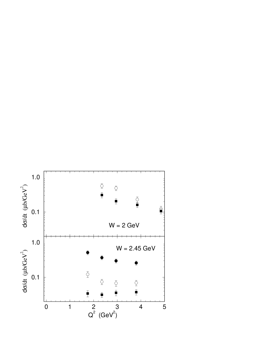
Figure 14: $d\sigma/dt$ at fixed values of $t$ and $W$, as a function of $Q^{2}$, for the reaction $\gamma^{*}p\to\omega p$ : $t=-0.55$ (full circles), $t=-1.45$ (empty circles) and $t=-2.30$ (squares) GeV².

3.4 $\phi$ dependence of cross sections

The 34 $\phi$ distributions have the expected $\phi$ dependence :

$$\frac{d\sigma}{d\phi}=\frac{1}{2\pi}\left(\sigma+\varepsilon\cos 2\phi\ \sigma_{TT}+\sqrt{2\varepsilon(1+\varepsilon)}\cos\phi\ \sigma_{TL}\right).$$ (5)

The interference terms $\sigma_{TT}$ and $\sigma_{TL}$ were extracted from a fit of each distribution with eq. (5). The results appear in fig. 15 and in table 3. If helicity were conserved in the $s$-channel (SCHC), these interference terms $\sigma_{TT}$ and $\sigma_{TL}$ would vanish. It does not appear to be the case in fig. 15. The $\phi$ distributions do not support the SCHC hypothesis.

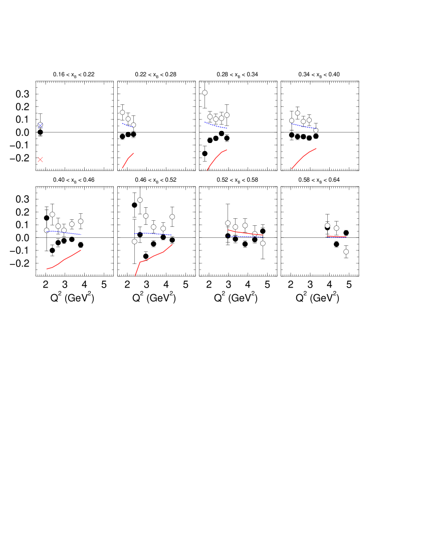
Figure 15: (Color online) $\sigma_{TT}$ (open circles) and $\sigma_{TL}$ (full circles), in units of $\mu$b, for the reaction $\gamma^{*}p\rightarrow\omega p$ as a function of $Q^{2}$ for different bins in $x_{B}$, integrated over $-2.7\ \hbox{GeV}^{2}<t<t_{0}$. The dashed blue and full red curves are the corresponding calculations in the JML model Lag04 discussed in sect. 5.

4 Analysis of $\omega$ decay distribution

In the absence of polarization in the initial state, the distribution of the pions from $\omega$ decay is characterized by eq. (4) Sch73 .

$$\mathcal{W}(\cos\theta_{N},\varphi_{N},\phi) = \frac{3}{4\pi}\displaystyle\left[\frac{1}{2}(1-r_{00}^{04})+\frac{1}{2}(3r_{00}^{04}-1)\cos^{2}\theta_{N}-\sqrt{2}\mbox{Re}r_{10}^{04}\sin 2\theta_{N}\cos\varphi_{N}-r_{1-1}^{04}\sin^{2}\theta_{N}\cos 2\varphi_{N}\right.$$

$$\hskip 19.91692pt-\varepsilon\cos 2\phi(r_{11}^{1}\sin^{2}\theta_{N}+r_{00}^{1}\cos^{2}\theta_{N}-\sqrt{2}\mbox{Re}r_{10}^{1}\sin 2\theta_{N}\cos\varphi_{N}-r_{1-1}^{1}\sin^{2}\theta_{N}\cos 2\varphi_{N})$$

$$\hskip 19.91692pt-\varepsilon\sin 2\phi(\sqrt{2}\mbox{Im}r_{10}^{2}\sin 2\theta_{N}\sin\varphi_{N}+\mbox{Im}r_{1-1}^{2}\sin^{2}\theta_{N}\sin 2\varphi_{N})$$

$$\hskip 19.91692pt+\sqrt{2\varepsilon(1+\varepsilon)}\cos\phi(r_{11}^{5}\sin^{2}\theta_{N}+r_{00}^{5}\cos^{2}\theta_{N}-\sqrt{2}\mbox{Re}r_{10}^{5}\sin 2\theta_{N}\cos\varphi_{N}-r_{1-1}^{5}\sin^{2}\theta_{N}\cos 2\varphi_{N})$$

$$\hskip 19.91692pt\left.+\sqrt{2\varepsilon(1+\varepsilon)}\sin\phi(\sqrt{2}\mbox{Im}r_{10}^{6}\sin 2\theta_{N}\sin\varphi_{N}+\mbox{Im}r_{1-1}^{6}\sin^{2}\theta_{N}\sin 2\varphi_{N})\displaystyle\right]$$

$$\mbox{where the parameters }r_{ij}^{\alpha}\mbox{, hereafter referred to as matrix elements, are related to the }\omega\mbox{ spin density matrix:}$$

$$r_{ij}^{04} = \frac{\rho_{ij}^{0}+\varepsilon R\rho_{ij}^{4}}{1+\varepsilon R};\hskip 28.45274ptr_{ij}^{\alpha}=\frac{\rho_{ij}^{\alpha}}{1+\varepsilon R}\mbox{ for }\alpha=1,2\ ;\hskip 28.45274ptr_{ij}^{\alpha}=\sqrt{R}\frac{\rho_{ij}^{\alpha}}{1+\varepsilon R}\mbox{ for }\alpha=5,6.$$ (7)

 

The quantities $\rho_{ij}^{\alpha}$ are defined from a decomposition of the $\omega$ spin density matrix on a basis of 9 hermitian matrices. The superscript $\alpha$ refers to this decomposition and it is related to the virtual photon polarization ($\alpha=0$–2 for transverse photons, $\alpha=4$ for longitudinal photons, and $\alpha=5$–6 for interference between $L$ and $T$ terms). For example, $\rho_{00}^{0}$ is related to the probability of the transition between a transverse photon and a longitudinal meson.

All elements $\rho_{ij}^{\alpha}$ can be expressed as bilinear combinations of helicity amplitudes which describe the $\gamma^{*}p\to\omega p$ transition Don02 ; Sch73 . An analysis of the $\mathcal{W}$ distribution can then be used to test whether helicity is conserved in the $s$-channel (SCHC), that is between the virtual photon and $\omega$. If SCHC applies, $\rho_{00}^{0}=0$ and $\rho_{00}^{4}=1$. Then eq. (7) leads to a direct relation between the measured $r_{00}^{04}$ and the ratio $R=\sigma_{L}/\sigma_{T}$. In that case, the longitudinal and transverse cross sections may be extracted from data without a Rosenbluth separation.

The matrix elements $r_{00}^{04}$ and $r_{1-1}^{04}$ were first extracted using one-dimensional projections of the $\mathcal{W}$ distribution. Note that $r_{1-1}^{04}$ should be zero if SCHC applies. Integrating eq. (4) over $\phi$ and then respectively over $\varphi_{N}$ or $\cos\theta_{N}$, one gets:

$$\mathcal{W}(\cos\theta_{N}) = \frac{3}{4}\left[(1-r_{00}^{04})+(3r_{00}^{04}-1)\cos^{2}\theta_{N}\right],$$ (8)

$$\mathcal{W}(\varphi_{N}) = \frac{1}{2\pi}\left[1-2r_{1-1}^{04}\cos 2\varphi_{N}\right].$$ (9)

The background subtraction in the $\cos\theta_{N}$ or $\varphi_{N}$ distributions was performed in 8 bins of the corresponding variables, and for 8 bins in ($Q^{2}$, $x_{B}$). The number of acceptance-weighted events was extracted from the corresponding $M_{X}[epX]$ distribution, as in sect. 2.3. See figs. 16 and 17 for results, together with fits to eqs. (8) and (9) respectively.

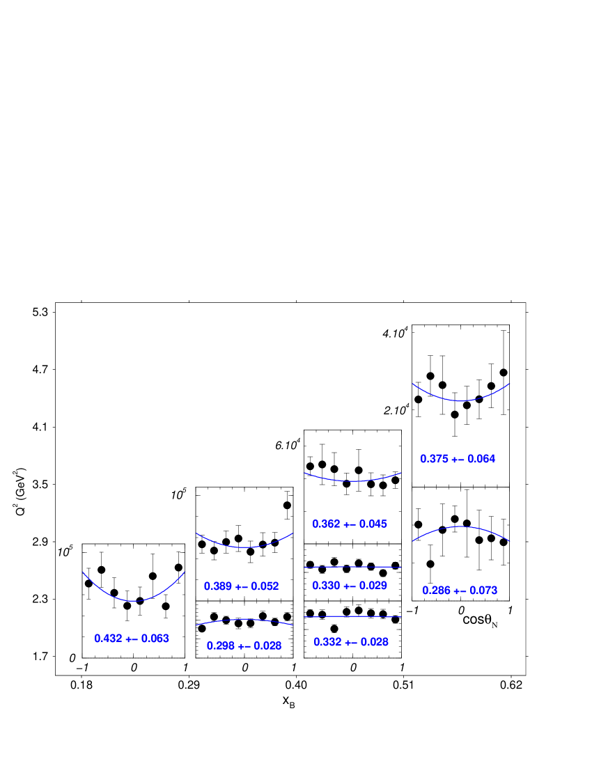
Figure 16: (Color online) Distributions of acceptance-weighted and background-subtracted counts as a function of $\cos\theta_{N}$, for 8 bins in ($Q^{2}$, $x_{B}$). The location and size of each graph correspond to the ($Q^{2}$, $x_{B}$) range over which the data is integrated. On all graphs, one division on the vertical axis represents $2\times 10^{4}$ (arbitrary units). All data are integrated in $t$ ($-t<2.7$ GeV²). The blue curves correspond to fits with eq. (8), with the resulting $r_{00}^{04}$ and its statistical uncertainty indicated on each distribution. The systematic uncertainty on this matrix element is estimated at 0.042.

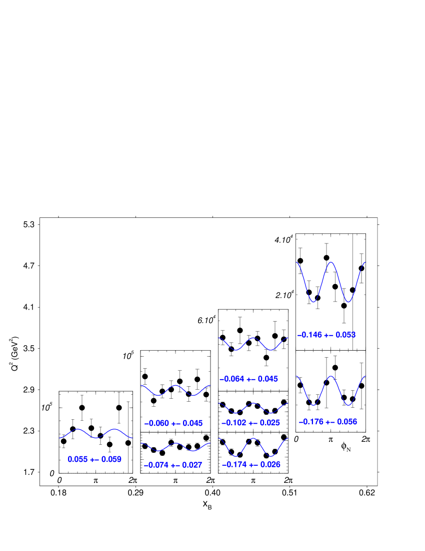
Figure 17: (Color online) Distributions of acceptance-weighted and background-subtracted counts as a function of $\varphi_{N}$. The blue curves correspond to fits with eq. (9), with the resulting $r_{1-1}^{04}$ and its statistical uncertainty indicated on each distribution. The systematic uncertainty on this matrix element is estimated at 0.042. See also legend of fig. 16.

Alternatively, the 15 matrix elements $r_{ij}^{\alpha}$ may be expressed in terms of moments of the decay distribution
$\mathcal{W}(\cos\theta_{N},\varphi_{N},\phi)$ Sch73 . This method of expressing moments includes the background contribution under the $\omega$ peak (about 25%). It yields compatible results with the (background subtracted) 1D projection method for $r_{00}^{04}$ and $r_{1-1}^{04}$. It was used to study the $t$ dependence of $r_{ij}^{\alpha}$ and to evaluate the systematic uncertainties in their determination. Results for forward $\gamma^{*}p\to\omega p$ reaction ($t^{\prime}<0.5$ GeV²) are given in fig. 18. Systematic uncertainties originate from the determination of the MC acceptance. The main source of uncertainties was found to be the finite bin size in $\phi$. Calculations with different bin sizes (see table 1) and checks of higher, unphysical, moments in the event distribution led to systematic uncertainties of 0.02 to 0.08, depending on the $r_{ij}^{\alpha}$ matrix element. In addition, cuts in the event weights were varied, resulting in a systematic uncertainty of about 0.03 for all matrix elements.

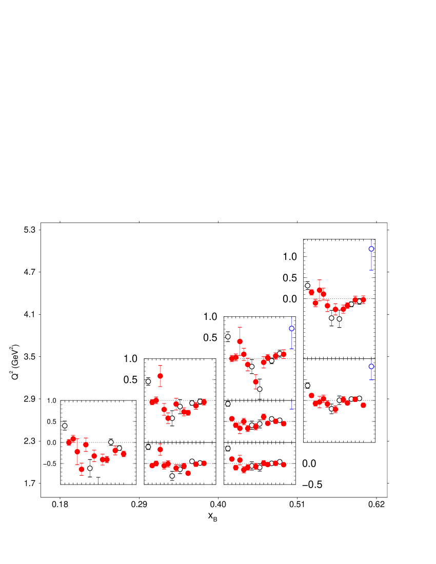
Figure 18: (Color online) $r_{ij}^{\alpha}$ extracted with the method of moments for 8 bins in ($Q^{2}$, $x_{B}$) and for $t^{\prime}<0.5$ GeV². The location and size of each graph correspond to the ($Q^{2}$, $x_{B}$) range over which the data is integrated, but the scale is the same on all graphs. The abscissa on each graph corresponds to the following list of matrix elements: $r_{00}^{04}$, Re $r_{10}^{04}$, $r_{1-1}^{04}$, $r_{00}^{1}$, $r_{11}^{1}$, Re $r_{10}^{1}$, $r_{1-1}^{1}$, Im $r_{10}^{2}$, Im $r_{1-1}^{2}$, $r_{00}^{5}$, $r_{11}^{5}$, Re $r_{10}^{5}$, $r_{1-1}^{5}$, Im $r_{10}^{6}$, Im $r_{1-1}^{6}$. The red filled symbols indicate those matrix elements which are zero if SCHC applies. The 16th entry (blue empty circle, in some cases off scale) is the combination of $r_{ij}^{\alpha}$ given by eq. (11). Error bars include systematic uncertainties added in quadrature.

Finally, the $r_{ij}^{\alpha}$ matrix elements were also extracted using an unbinned maximum likelihood method. Results were compatible with the first two methods. In view of the $\phi$ dependence of the acceptance (see fig. 9), this method was used for checking the validity of the $r_{ij}^{\alpha}$ determination when restricting the $\phi$ range taken into consideration in the fit.

These studies lead to the conclusion that SCHC does not hold for the reaction $\gamma^{*}p\to\omega p$, not only when considering the whole $t$ range (fig. 17), but also, though in a lesser extent, in the forward direction (fig. 18). For SCHC, all matrix elements become zero, except five: $r_{00}^{04}$, $r_{1-1}^{1}$, Im $r_{1-1}^{2}$, Re $r_{10}^{5}$, Im $r_{10}^{6}$ and these are not all independent; they satisfy Don02 : $r_{1-1}^{1}=-$Im$r_{1-1}^{2}$ and Re$r_{10}^{5}=-$Im$r_{10}^{6}$. The quantity

$$\chi^{2}=\frac{1}{12}\left[\sum_{1}^{10}\left(\frac{r}{\Delta r}\right)^{2}\right. +\frac{(r_{1-1}^{1}+\mbox{Im}r_{1-1}^{2})^{2}}{(\Delta r_{1-1}^{1})^{2}+(\Delta\mbox{Im}r_{1-1}^{2})^{2}}$$

$$+ \left.\frac{(\mbox{Re}r_{10}^{5}+\mbox{Im}r_{10}^{6})^{2}}{(\Delta\mbox{Re}r_{10}^{5})^{2}+(\Delta\mbox{Im}r_{10}^{6})^{2}}\right]$$ (10)

where the sum is carried over the ten matrix elements which would be zero if SCHC applies, may be used as a measure of SCHC violation. Including in the denominators $\Delta r$ the systematic uncertainties added in quadrature to the statistical uncertainties, the 7 $\chi^{2}$ values (excluding the distributions at the lowest $x_{B}$ bin where SCHC violation is the most manifest in fig. 18) range from 2.3 to 7.7 when including all data, and drop only to 1.7 to 5.1, in spite of doubled statistical uncertainties, when considering only the forward production ($t^{\prime}<0.5$ GeV²). Furthermore, when examining the relation between these matrix elements and helicity-flip amplitudes, it does not appear possible to ascribe the SCHC violation to a small subset of these amplitudes. It is therefore not justified to calculate $R$ from eq. (7) and separate the longitudinal and transverse cross sections from this data.

When one retains only those amplitudes which correspond to a natural parity exchange in the $t$-channel, then the following relation should hold Tyt01  :

$$1-r_{00}^{04}+2r_{1-1}^{04}-2r_{11}^{1}-2r_{1-1}^{1}=0$$ (11)

This particular combination is plotted as the 16th point on each of the graphs of fig. 18. The fact that it is not zero points to the importance of the unnatural parity (presumably pion) exchange.

It is also possible to estimate qualitatively the role of pion exchange through the U/N asymmetry of the transverse cross section, where U and N refer to unnatural and natural parity exchange contributions Don02 :

$$P\equiv\frac{\sigma_{T}^{N}-\sigma_{T}^{U}}{\sigma_{T}^{N}+\sigma_{T}^{U}}=(1+\varepsilon R)(2r_{1-1}^{1}-r_{00}^{1})\ .$$ (12)

Our results yield $r_{1-1}^{1}<0$ and $r_{00}^{1}\geq 0$ over the whole kinematical range, and thus:

$$P<-(2|r_{1-1}^{1}|+|r_{00}^{1}|)\ .$$ (13)

Hence $P$ is large and negative, which means that most of the transverse cross section is due to unnatural parity exchange.

5 Comparison with a Regge model

Regge phenomenology was applied with success to the photoproduction of vector mesons in our energy range and at higher energies Can02 ; Sib03 . Laget and co-workers showed that the introduction of saturating Regge trajectories provides an excellent simultaneous description of the high $-t$ behaviour of the $\gamma p\to p\rho,\omega,\phi$ cross sections, given an appropriate choice of the relevant coupling constants. The $t$-channel exchanges considered in this JML model are indicated in table 4. Saturating trajectories have a close phenomenological connection to the quark-antiquark interaction which governs the mesonic structure Ser94 . They provide an effective way to implement gluon exchange between the quarks forming the exchanged meson.

Table 4: Meson and Pomeron (or two-gluon) exchanges considered in the JML model for vector meson production.

Produced	Exchanged
vector meson	Regge trajectories
$\rho$	$\sigma$, $f_{2}$, P/2g
$\omega$	$\pi^{0}$, $f_{2}$, P/2g
$\phi$	P/2g

This model was extended to the case of electroproduction Lag04 . The $Q^{2}$ dependence of the $f_{2}$ and P exchange is built in the model. In the case of $\omega$ production, the only additional free parameters come from the electromagnetic form factor which accounts for the finite size of the vertex between the virtual photon, the exchanged $\pi^{0}$ trajectory and the $\omega$ meson. This form factor could be chosen as the usual parameterization of the pion electromagnetic form factor: $F_{\omega\pi\gamma}=F_{\pi}=(1+Q^{2}/\Lambda_{\pi}^{2})^{-1}$, with $\Lambda_{\pi}^{2}=0.462$ GeV². As described so far, the model fails to account for the observed $t$ dependence (see dashed lines in fig. 12). From the observation that the differential cross section becomes nearly $Q^{2}$-independent at high $-t$, an adhoc modification of the form factor

$$F_{\omega\pi\gamma}(Q^{2})\to F_{\omega\pi\gamma}(Q^{2},t)=\frac{1}{1+\frac{Q^{2}}{\Lambda_{\pi}^{2}}\left(\frac{1+\alpha_{\pi}(t)}{1+\alpha_{\pi}(0)}\right)^{2}}$$ (14)

was proposed Lag04 . The saturating $\pi^{0}$ Regge trajectory obeys the relation $\lim_{t\to-\infty}\alpha_{\pi}(t)=-1$, so that the form factor becomes flat at high $-t$. Thus, eq. (14) associates the point-like coupling of the virtual photon with the saturation of the $\pi^{0}$ Regge trajectory which accounts for hard scattering in this kinematical limit Lag04 . Note that this modification of the form factor does not violate gauge invariance, which holds separately for each contribution from Table 4 and, in the case of $\pi^{0}$ exchange, from the spin and momentum structure of the $\omega\pi\gamma$ vertex.

The $t$ dependence of the differential cross sections is then well described (solid lines in fig. 12). The $Q^{2}$ dependence of the cross sections is illustrated in fig. 10. At high $x_{B}$, which corresponds to the lowest values of $W$, $s$-channel resonance contributions are not taken into account in the model and may explain the observed disagreement. Finally the interference terms $\sigma_{TT}$ and $\sigma_{TL}$ agree in sign and trend, but not in magnitude, with our results (fig. 15).

So, within this model, $\pi^{0}$ exchange, or rather the exchange of the associated saturating Regge trajectory, continues to dominate the cross section at high $Q^{2}$ and the cross section is mostly transverse. This is consistent with our observations of the dominance of unnatural parity exchange in the $t$-channel in the previous section.

6 Relevance of the handbag diagram

Let us recall that the handbag diagram of fig. 1 is expected to be the leading one in the Bjorken regime. In this picture, the transition $\gamma^{*}_{L}\to\omega_{L}$ would dominate the process. This is clearly antinomic to the findings in sect. 5, where our results are interpreted as dominated by the $\pi^{0}$ exchange, which is mostly due to transverse photons. In addition, $\pi^{0}$ exchange is of a pseudo-scalar nature, while the $H$ and $E$ GPD which enter the handbag diagram amplitude are of a vector nature.

Independent of the model interpretation presented in sect. 5, our results point to the non-conservation of helicity in the $s$-channel (figs. 15, 17 and 18), meaning that the handbag diagram does not dominate the process, even for small values of $-t$ and $Q^{2}$ as large as 4.5 GeV².

As a consequence, $\sigma_{L}$ could not be extracted from our data for a direct comparison with models based on the GPD formalism. It is however instructive to consider here the predictions of a GPD-based model Vdh97 ; Goe01 , denoted hereafter VGG. This is a twist-2, leading order calculation, where the GPD are parameterized in terms of double distributions ($DD$) and include the so-called D-term (see Ref. Goe01 for definitions): $H,E\sim DD(x,\xi)e^{b(\xi,Q^{2})t/2}$, where $b$ is taken from the data (see sect. 3.3 and table 3). An effective way of incorporating some of the higher twist effects is to introduce a “frozen” strong coupling constant $\alpha_{S}=0.56$. This model is described in some more details in Ref. Had04 and is applied here to the specific case of $\omega$ production. The model calculations (VGG and JML) of $\varepsilon\sigma_{L}$ are plotted in fig. 19. The sharp drop of the curves at high $Q^{2}$ is due to the decrease of $\varepsilon$, at our given beam energy, as $Q^{2}$ reaches its kinematical limit. When compared to our results, $\varepsilon\sigma_{L}$ is calculated to be only 1/6 to 1/4 of the measured cross sections, thus explaining the difficulty in extracting this contribution.

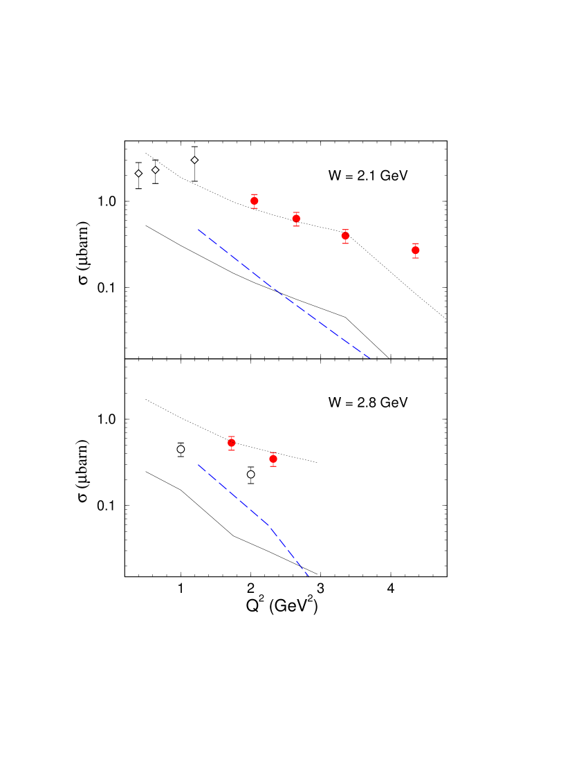
Figure 19: (Color online) Total cross sections for the reaction $\gamma^{*}p\to\omega p$, for $\langle W\rangle=$ 2.1 (top) and 2.8 (bottom) GeV : this work (full red circles), DESY data (empty diamonds), Cornell data (empty circles), and JML model (dotted curves). The longitudinal contribution, $\varepsilon(E,Q^{2})\sigma_{L}$, is calculated according to the JML (solid lines) and VGG (dashed blue lines) models.

The $\omega$ channel thus appears to be a challenging reaction channel to study the applicability of the GPD formalism. This is attributed to the $t$-channel $\pi^{0}$ exchange, which remains significant even at high values of $Q^{2}$. In contradistinction, the $\pi^{0}$ exchange is negligible in the case of the $\rho$ production channel, where SCHC was found to hold, and $\sigma_{L}$ could be extracted and compared successfully to GPD models Air00 ; Had04 .

7 Summary

An extensive set of data on exclusive $\omega$ electroproduction has been presented, for $Q^{2}$ from 1.6 to 5.1 GeV² and $W$ from 1.8 to 2.8 GeV ($x_{B}$ from 0.16 to 0.64). Total and differential cross sections for the reaction $\gamma^{*}p\to\omega p$ were extracted, as well as matrix elements linked to the $\omega$ spin density matrix.

The $t$ differential cross sections are surprisingly large for high values of $-t$ (up to 2.7 GeV²). This feature can be accounted for in a Regge-based model (JML), provided a $t$ dependence is assumed for the $\omega\pi\gamma$ vertex form factor, with a prescription inspired from saturating Regge trajectories. It appears that the virtual photon is more likely to couple to a point-like object as $-t$ increases.

The analysis of the $\phi$ differential cross sections and of the $\omega$ decay matrix elements indicate that the $s$-channel helicity is not conserved in this process. As a first consequence, the longitudinal and transverse contributions to the cross sections could not be separated. Furthermore, the values of some decay matrix elements point to the importance of unnatural parity exchange in the $t$-channel, such as $\pi^{0}$ exchange. This behaviour had been previously established in the case of $\omega$ photoproduction, but not for the large photon virtuality obtained in this experiment. The results on these observables also support the JML model, where the exchange of the saturating Regge trajectory associated with the $\pi^{0}$ is mostly transverse and dominates the process.

Finally, the experiment demonstrated that exclusive vector meson electroproduction can be measured with high statistics in a wide kinematical range. The limitations at high $Q^{2}$ were not due to the available luminosity of the CEBAF accelerator or to the characteristics of the CLAS spectrometer, but to the present beam energy. With the planned upgrade of the beam energy up to 12 GeV upgrade , such reactions will be measured to still higher values of $Q^{2}$. In the specific case of the $\omega$ meson, as was shown in this paper, this will be a necessary condition for the extraction of a longitudinal contribution of the handbag type, related at low values of $-t$ to generalized parton distributions. More generally, this experiment opens a window on the high $Q^{2}$ and high $-t$ behaviour of exclusive reactions, which needs further exploration.

- (1) T.H. Bauer et al., Rev. Mod. Phys. 50 (1978) 261.
- (2) L.L. Frankfurt, G.A. Miller and M.I. Strikman, Ann. Rev. Nucl. Sci. 44 (1994) 501.
- (3) M. Vanderhaeghen, P.A.M. Guichon and M. Guidal, Phys. Rev. D 56 (1997) 2982.
- (4) F. Cano and J.-M. Laget, Phys. Rev. D 65 (2002) 074022.
- (5) S. Donnachie, G. Dosch, P. Landshoff and O. Nachtmann, Pomeron Physics and QCD (Cambridge University Press, New York, 2002).
- (6) J.-M. Laget, Phys. Lett. B489 (2000) 313.
- (7) M. Battaglieri et al., Phys. Rev. Lett. 90 (2003) 022002.
- (8) X. Ji, Phys. Rev. Lett. 78 (1997) 610; Phys. Rev. D 55 (1997) 7114; Annu. Rev. Nucl. Part. Sci. 54 (2004) 413.
- (9) A.V. Belitsky and A.V. Radyushkin, Report JLAB-THY-04-34 (2004), hep-ph/0504030.
- (10) J.C. Collins, L. Frankfurt, and M. Strikman, Phys. Rev. D 56 (1997) 2982.
- (11) A. Airapetian et al., Eur. Phys. J. C 17 (2000) 389.
- (12) C. Hadjidakis et al., Phys. Lett. B 605 (2005) 256.
- (13) M. Diehl, Phys. Rep. 388 (2003) 41.
- (14) J. Ballam et al., Phys. Rev. D 10 (1974) 765.
- (15) C. del Papa et al., Phys. Rev. D 19 (1979) 1303.
- (16) P. Joos et al., Nucl. Phys. B122 (1977) 365.
- (17) D.G. Cassel et al., Phys. Rev. D 24 (1981) 2787.
- (18) J. Breitweig et al., Phys. Lett. B 487 (2000) 273.
- (19) M. Tytgat, DESY-THESIS-2001-018 (2001).
- (20) A.H. Rosenfeld and P. Söding, Properties of the fundamental interactions, in Proceedings 1971 Int. School of Subnuclear Physics, Erice, edited by A. Zichichi, Vol. 9C (Editrice Compositori, Bologna, 1973) p. 883.
- (21) L. Morand, Thèse de doctorat, Université Denis Diderot-Paris 7 (2003); Report DAPNIA-03-09-T.
- (22) M.L. Stevenson et al., Phys. Rev. 125 (1962) 687.
- (23) B.A. Mecking et al., Nucl. Instr. and Meth. A503 (2003) 513.
- (24) A separate CLAS experiment, under analysis, addresses the low and low electroproduction; see V. Burkert et al., AIP Conf. Proc. 549 (2002) 259.
- (25) P. Corvisiero et al., Nucl. Instr. and Meth. A346 (1994) 433; and M. Battaglieri, private communication.
- (26) L.W. Mo and Y.S. Tsai, Rev. Mod. Phys. 41 (1969) 205.
- (27) L.N. Hand, Phys. Rev. 129 (1963) 1834.
- (28) Particle Data Group: S. Eidelman et al., Phys. Lett B592 (2004) 1.
- (29) J.-M. Laget, Phys. Rev. D 70 (2004) 054023.
- (30) K. Schilling and G. Wolf, Nucl. Phys. B61 (1973) 381.
- (31) A. Sibirtsev, K. Tsushima and S. Krewald, Phys. Rev. C 67 (2003) 055201.
- (32) M.N. Sergeenko, Z. Phys. C64 (1994) 315.
- (33) K. Goeke, M.V. Polyakov and M. Vanderhaeghen, Prog. Part. Nucl. Phys. 47 (2001) 401.
- (34) Pre-conceptual design report for the science and experimental equipment for the 12 GeV upgrade of CEBAF, http://www.jlab.org/div_dept/physics_division/ pCDR_public/pCDR_final