Abstract

We present a measurement of the top pair production cross section in ${p\bar{p}}$ collisions at $\sqrt{s}$=1.96 TeV. We collect a data sample with an integrated luminosity of 194$\pm$11 pb^-1 with the CDF II detector at the Fermilab Tevatron. We use an artificial neural network technique to discriminate between top pair production and background processes in a sample of 519 lepton+jets events, which have one isolated energetic charged lepton, large missing transverse energy and at least three energetic jets. We measure the top pair production cross section to be $\sigma_{t\overline{t}}=6.6$$\pm 1.1\pm 1.5$ pb, where the first uncertainty is statistical and the second is systematic.

I Introduction

We report on a measurement with the Collider Detector at the Fermilab Tevatron of the rate of pair production of top quarks in the lepton+jets channel, ${p\bar{p}}\rightarrow{t\bar{t}}\rightarrow W^{+}W^{-}b\bar{b}\rightarrow\ell\bar{\nu_{\ell}}q\bar{q^{\prime}}b\bar{b}$. Recent theoretical calculations predict the cross section for top pair production mlm ; kidonakis with an uncertainty of less than 15%. The increase in the Fermilab Tevatron center-of-mass energy to 1.96 TeV from 1.80 TeV is expected to have enhanced the top pair production cross section by 30%. Each top quark is expected to decay into a $W$ boson and a $b$ quark, with a branching fraction of almost 100%. A significant deviation of the observed rate of top pair production from the standard model prediction could indicate either a novel top quark production mechanism, e.g. the production and decay of a heavy resonance into ${t\bar{t}}$ pairs heavyresonance , or a novel top quark decay mechanism, e.g. a decay into supersymmetric particles supersymmetry , or a similar final state signature from a top-like particle tprime ; tprime1 ; beautmirrors ; littlehier . Previous measurements of the properties of the top quark topProperties are consistent with expectations from the standard model but suffer from large statistical uncertainties.

We first show that it is feasible to measure the top pair production cross section with a single kinematic event property, which may be used to discriminate between the signal from top pair production and the dominant background from $W$ boson production with associated jets KinEvidence . This property is the total transverse energy in the event Htfirst , which has been used as a discriminant by several recent top analyses ttbardilepton ; svxruniipaper ; sltpaper . In addition, we test the modeling of the kinematics of top pair and $W+$jets production. A good understanding of the kinematics of these processes will be required to discover single top quark production and will benefit searches for the Higgs boson and physics beyond the standard model at both the Tevatron and the future Large Hadron Collider, where techniques using kinematic discrimination have been proposed.

We then develop an artificial neural network technique in order to maximize the discriminating power available from kinematic and topological properties KinStudiesRun1 . Throughout this paper, we quantify the gain of our neural network approach relative to the single event property of total transverse energy. The statistical sensitivity of our neural network technique is comparable to that of methods employing secondary vertex $b$-tagging svxruniipaper ; Taka+Mel , and is independent of the assumptions and systematic uncertainties specific to $b$-tagging.

II Experimental Apparatus

The Collider Detector at Fermilab (CDF) has been substantially upgraded for the current Tevatron collider run, which began in 2001. The major upgrades include new charged particle tracking detectors, forward calorimetry, trigger and data acquisition electronics and infrastructure as well as extended muon coverage. A thorough description of the detector is provided elsewhere cdfdetector . The essential components of the detector for this analysis are briefly described here.

The reconstruction of charged particles with high transverse momentum is essential to the electron and muon triggers that collect our data sample, the identification of electrons and muons, and the measurement of the muon momentum. The charged particle tracking detectors are immersed in a 1.4 T magnetic field from a superconducting solenoid, which is oriented parallel to the proton beam direction itsthegeometrystupid . The Central Outer Tracker cotref (COT) has eight super-layers of 310 cm long wires covering radii from 40 to 137 cm. Each super-layer consists of planes of 12 sense wires. The super-layers alternate between having wires parallel to the cylinder axis and wires displaced by a $2^{\circ}$ stereo angle. This provides three dimensional charged particle track reconstruction, with up to 96 position measurements with a spatial resolution of about 180 $\mathrm{\mu}$m in the transverse plane. The COT transverse momentum resolution is $\sigma_{p_{T}}/p^{2}_{T}\approx 0.0017$ $\mathrm{[GeV/c]^{-1}}$. The inner tracking detector is a silicon strip detector L00 ; svxref ; ISL that provides up to eight position measurements with a spatial resolution of about 15 $\mathrm{\mu}$m.

Calorimetry is used to measure the transverse energy of electrons and jets, as well as to infer the presence of neutrinos from a significant imbalance in the observed transverse energy. The calorimeters lie outside the solenoid and are physically divided into a central region CEM ; CHA covering pseudo-rapidity $|\eta|<1.1$ and an upgraded plug region PEM covering $1.1<|\eta|<3.6$. The electromagnetic calorimeter is a lead-scintillator sandwich, which is 18 radiation lengths deep in the central region (CEM), with energy resolution of $14\%/\sqrt{E_{T}}$. The hadronic calorimeter is an iron-scintillator sandwich, which is 4.5 nuclear interaction lengths deep in the central region (CHA), with energy resolution of $50\%/\sqrt{E}$. The calorimeters are segmented into a projective “tower” geometry, where each tower subtends an area of 0.11 in $\eta$ and 15^∘ in azimuth in the central region. Finer position resolution for electron and photon identification is provided by proportional chambers (CES), located at the approximate electromagnetic shower maximum depth in each tower.

Muons are identified in drift chambers which surround the calorimeters up to $|\eta|<1.0$. The Central Muon Detector (CMU) CMU consists of a set of drift chambers located outside the central hadronic calorimeters and covers $|\eta|<0.6$. An additional 60 cm thick layer of steel shields the four layers of single wire drift tubes that comprise the Central Muon Upgrade detector (CMP). The Central Muon Extension detector (CMX) consists of drift tubes, located at each end of the central detector between $42^{\circ}-55^{\circ}$ in polar angle, that extend the coverage to muons between $0.6<\eta<1.0$.

Gas Cerenkov light detectors CLC located in the $3.7<|\eta|<4.7$ region measure the number of inelastic $p\bar{p}$ collisions per bunch crossing and thereby the luminosity delivered to CDF by the Tevatron. The total uncertainty on the luminosity is 5.9%, where 4.4% comes from the acceptance and operation of the luminosity monitor and 4.0% from the calculation of the total $p\bar{p}$ cross section cdflumi .

III Selection of data sample

Top quark events in the lepton+jets channel, ${p\bar{p}}\rightarrow{t\bar{t}}\rightarrow\ell\bar{\nu_{\ell}}q\bar{q^{\prime}}b\bar{b}$, are characterized by a high transverse momentum lepton and substantial missing transverse energy due to the leptonic $W$ decay along with several hadronic jets with high transverse energy. Two jets are expected from the hadronic $W$ decay, two more are expected from the $b$ and $\overline{b}$ quarks originating from the respective $t$ and $\bar{t}$ decays. In practice, not all of these jets may be reconstructed due to kinematic requirements and limitations of the detector geometry, while other jets may arise from initial and final state hard radiation effects.

The data sample in this paper is collected by a trigger based solely on the presence of a high transverse momentum lepton. In this section, we discuss the trigger and lepton identification requirements, the reconstruction of the jets and the missing transverse energy, and further requirements we impose to reduce specific backgrounds. The same criteria are applied to both data and Monte Carlo simulation.

III.1 Data

This analysis uses data from $p\bar{p}$ collisions at a center-of-mass energy of $\sqrt{s}=1.96$ TeV collected with CDF between March 2002 and September 2003. All of the detector subsystems important for lepton identification and kinematic reconstruction, namely the central outer tracker, calorimeters and muon chambers, were carefully monitored over this period and any segment of data with a problem in any of these systems was excluded from consideration. No requirement was made on the silicon detectors for this analysis. The integrated luminosity of this data sample was measured to be 194$\pm$11 pb^-1 cdflumi .

III.2 Trigger

CDF uses a three-level trigger and data acquisition system to filter interesting events from the 1.7 MHz beam crossing rate and write them to permanent storage at an average rate of 60 Hz. We describe here only the triggers important for this analysis, which select events containing an electron or muon with high transverse momentum ($p_{T}$). The efficiencies of these triggers have been measured directly from the data wzprd and are listed in Table 6.

At the first level (L1), charged particle tracks reconstructed in the COT $r-\phi$ projection by a hardware track processor, the eXtremely Fast Tracker (XFT) xftref , are required to point to a cluster of energy in the electromagnetic calorimeter or to a track segment in the muon chambers. The L1 electron trigger requires an XFT track with $p_{T}>8$ GeV/$c$, matched to a single trigger tower in the central electromagnetic calorimeter having transverse energy $E_{T}>8$ GeV and with a ratio of hadronic to electromagnetic energy less than 0.125. The L1 muon trigger requires that either an XFT track with $p_{T}>4$ GeV/$c$ be matched to a muon track segment with $p_{T}>6$ GeV/$c$ from the CMU and the CMP, or that an XFT track with $p_{T}>8$ GeV/$c$ be matched to a muon track segment with $p_{T}>6$ GeV/$c$ from the CMX.

The second level (L2) electron trigger requires the XFT track matched to a cluster of energy in the central electromagnetic calorimeter with $E_{T}>16$ GeV and with a ratio of hadronic to electromagnetic energy less than 0.125. The calorimeter cluster is formed by adding the energy in neighboring trigger towers with $E_{T}>7.5$ GeV to the original L1 trigger tower. For this data set, the L2 muon trigger automatically accepts events passing the L1 muon trigger.

At the third level (L3), a farm of Linux computers performs on-line a complete event reconstruction, including three-dimensional charged particle track reconstruction. The L3 electron trigger requires: a track with $p_{T}>9$ GeV/$c$ matched to a cluster of energy in three adjacent towers in pseudo-rapidity in the central electromagnetic calorimeter with $E_{T}>18$ GeV; the ratio of hadronic to electromagnetic energy less than 0.125; a lateral shower profile of the calorimeter cluster less than 0.4; and the distance between the extrapolated track position and the CES measurement in the $z$ view less than 10 cm. The L3 muon trigger requires a track with $p_{T}>18$ GeV/$c$ matched to a track segment in the muon chambers within $10$ cm in the $r-\phi$ view and, for CMU and CMP muons only, within $20$ cm in the $z$ view.

III.3 Electron identification

Electron candidates are required to have a COT track with $p_{T}>9$ GeV/$c$ that extrapolates to a cluster of energy with $E_{T}>20$ GeV formed by three adjacent towers in pseudo-rapidity in the central electromagnetic calorimeter. The electron energy is corrected by less than 5% for the non-uniform response across each calorimeter tower by using the CES measurement of the shower position. The shower position is required to be away from the calorimeter tower boundaries to ensure high quality discrimination between electrons and charged hadrons. This fiducial volume for electrons covers 84% of the solid angle in the central $|\eta|<1.0$ region. The selection requirements are defined below and listed in Table 1:

• Ratio of hadronic energy in the cluster, $E_{\textrm{h}ad}$, to the electromagnetic energy in the cluster, $E_{\textrm{e}m}$.

• Comparison of the lateral shower profile lshr , the distribution of adjacent CEM tower energies as a function of the seed tower energy in the calorimeter, with that expected from test beam electrons, $L_{\textrm{shr}}$.

• $\chi^{2}$ comparison of the CES shower profiles with those of test beam electrons in the $z$ view, $\chi^{2}_{\textrm{strip}}$.

• Distance between the position of the extrapolated track and the CES shower profiles measured in the $r-\phi$ and $z$ views, $\Delta x$ and $\Delta z$. The limits on $\Delta x$ are asymmetric and signed by electric charge $Q$ to allow for energy deposition from bremsstrahlung photons emitted as the electron/positron passes through the detector material.

• Ratio of cluster energy to track momentum, $E/P$.

• Isolation, $I$, defined as the ratio between any additional transverse energy in a cone of radius $R=\sqrt{(\delta\eta)^{2}+(\delta\phi)^{2}}=0.4$ around the cluster and the transverse energy of the cluster.

Table 1: Selection requirements for electron candidates from $W$ boson decay.

Property	Requirement
$E_{T}$	$\geq$ 20 GeV
$E_{\textrm{had}}/E_{\textrm{em}}$	$\leq$ 0.055+0.00045*E (GeV)
$L_{\textrm{shr}}$	$\leq$ 0.2
$\chi^{2}_{\textrm{strip}}$	$\leq$ 10.0
$|\Delta z|$	$\leq$ 3.0 cm
$Q*\Delta x$	$\geq$ -3.0 cm, $\leq$ 1.5 cm
$E/P$	$\leq$ 2.0 or $p_{T}>50$ GeV/$c$
Isolation	$\leq$ 0.1
Conversion	Veto

For electrons in the fiducial volume, the identification efficiency is determined from a data sample of $Z\to e^{+}e^{-}$ events and is found to be 82.5 $\pm$ 0.5%, where the uncertainty is statistical only. In our estimate of the selection efficiency for top pair events, we are sensitive to systematic differences in electron identification between data and simulation. We use $Z\to e^{+}e^{-}$ data and simulation samples to measure a correction factor of 0.965$\pm$0.014 for the electron identification efficiency, where the uncertainty is statistical only. We discuss systematic uncertainties and differences between the electron environment in $Z\to e^{+}e^{-}$ events and ${t\bar{t}}$ events further in section VIII.

Photon conversions occur throughout the detector material and are a major source of electrons and positrons that pass the above selection criteria. We identify photon conversions by the characteristic small opening angle between two oppositely charged tracks that are parallel at their distance of closest approach to each other. Specifically, we require the distance between the tracks in the $r-\phi$ plane at the radius where the tracks are parallel to be less than 0.2 cm, and the difference between the cotangent of polar angles to be less than 0.04. We reject electron candidates with an oppositely charged partner track meeting these requirements. In this analysis, we are sensitive to any loss in efficiency from the mis-identification of an electron from $W$ boson decay as a photon conversion. We measure the loss in efficiency with a $Z\rightarrow e^{+}e^{-}$ data sample. We find that we can halve the loss in efficiency to $2.3\pm 0.04$% by not rejecting electrons accompanied by a converted bremsstrahlung photon. Specifically, we do not reject electron candidates where the nearby oppositely charged particle track itself has an additional conversion partner. For completeness, we note here that the performance of this algorithm to identify electrons from photon conversions is estimated svxruniipaper at $72.6\pm 0.07$%, where the error covers both statistical and systematic uncertainties.

III.4 Muon identification

Muon candidates are required to have a COT track with $p_{T}>20$ GeV/$c$ that extrapolates to a track segment in the muon chambers. The muon COT track curvature, and thus the muon transverse momentum, is corrected in order to remove a small azimuthal dependence from residual detector alignment effects wzprd . The selection requirements used to separate muons from products of hadrons that interact in the calorimeters and from cosmic rays are defined below and listed in Table 2:

• Energy deposition in the electromagnetic and hadronic calorimeter expected to be characteristic of minimum ionizing particles, $E_{\textrm{em}}$ and $E_{\textrm{had}}$.

• Distance between the extrapolated track and the track segment in the muon chamber, $\Delta x$. A track matched to a segment in the CMU muon chambers is required to have a matched track segment in the CMP chambers as well, and vice versa.

• Distance of closest approach of the reconstructed track to the beam-line in the transverse plane, $d_{0}$. If available, information from the silicon tracking detector is included to increase precision and improve rejection of muons from cosmic rays and decays-in-flight of charged hadrons.

• Cosmic ray muons that pass through the detector close to the beam-line may be reconstructed as a pair of charged particles. We use the timing capabilities of the COT to reject events where one of the tracks from a charged particle appears to travel toward instead of away from the center of the detector.

• Isolation, $I$, defined as the ratio between any additional transverse energy in a cone of radius $R=0.4$ around the track direction and the muon transverse momentum.

Table 2: Selection requirements for muon candidates from $W$ boson decay.

Property	Requirement
$p_{T}$	$\geq$ 20 GeV
$E_{\textrm{h}ad}$	$\leq\max(6,6+0.0280(p-100))$ GeV
$E_{\textrm{e}m}$	$\leq\max(2,2+0.0115(p-100))$ GeV
${\textrm{C}MU}|\Delta x|$	$\leq$ 3.0 cm
${\textrm{C}MP}|\Delta x|$	$\leq$ 5.0 cm
${\textrm{C}MX}|\Delta x|$	$\leq$ 6.0 cm
$|d_{0}|$	$\leq$ 0.02 cm (0.2 cm) with (without) silicon tracking
Isolation	$\leq$ 0.1
Cosmic ray	Veto

The identification efficiency is determined from a data sample of $Z\to\mu^{+}\mu^{-}$ events and is found to be 85.1 $\pm$ 0.7% for muons fiducial to CMU/CMP and 90.1 $\pm$ 0.8% for muons fiducial to CMX, where the uncertainty is statistical only. In our estimate of the selection efficiency for top pair events, we are sensitive to systematic differences in muon identification between data and simulation. We use $Z\to\mu^{+}\mu^{-}$ data and simulation samples to measure correction factors of 0.887$\pm$0.014 for CMU/CMP and 1.001$\pm$0.017 for CMX muon identification efficiencies, where the uncertainty is statistical only. We discuss systematic uncertainties and differences between the muon environment in $Z\to\mu^{+}\mu^{-}$ events and ${t\bar{t}}$ events further in section VIII.

III.5 Track quality and primary vertex reconstruction

For both electron and muon candidates, the charged particle track is required to have at least 3 axial and 3 stereo COT super-layer track segments, with each segment having at least 7 hits attached out of a possible total of 12 hits. We constrain the COT track fit to be consistent with the beam position in the transverse plane. We use an unbiased data sample collected by a calorimeter-only trigger to calibrate the track reconstruction efficiency for isolated leptons and we find a correction factor of 1.009 $\pm$ 0.002 to the simulation efficiency.

We reconstruct the $z$ position of each primary interaction using an algorithm based on COT and silicon tracking information. Since there may be multiple $p\overline{p}$ interactions, we identify the $z$ coordinate of the event with the $z$ position of the reconstructed primary vertex closest to the lepton COT track $z$ position, $z_{0}$, at its point of closest approach to the beam-line in the transverse plane. In less than 1% of the cases the separation is greater than 5 cm, so we use instead the $z_{0}$ of the lepton COT track as the event $z$ position.

We require the $z$ position of the event to be within $60$ cm of the center of the detector, in order to ensure good event reconstruction in the projective tower geometry of the CDF calorimeter. However, the integrated luminosity of the data sample is measured for the full $p\bar{p}$ luminous region, which extends beyond this range. Our simulation attempts to model the $z$ profile of the $p\bar{p}$ luminous region but may not be correct on average. Therefore, we estimate the selection efficiency for top pair events in simulation with respect to events that have a $z$ position in this range. We use minimum bias data to find that this range covers $94.8\pm 0.3$% of the full $p\bar{p}$ luminous region. We then apply this number as a correction factor to our estimate of the selection efficiency for top pair events.

III.6 Jet reconstruction and systematic uncertainties

This analysis is heavily dependent on jet-based kinematic properties to discriminate between signal and background processes. Therefore we discuss here the reconstruction of jets and the uncertainties related to the jet energy scale ARun1Paper .

The jets used in this analysis are reconstructed from calorimeter towers using a cone algorithm JETCLUref with a radius $R=\sqrt{(\Delta\phi)^{2}+(\Delta\eta)^{2}}\leq$0.4, where the $E_{T}$ of each tower is calculated with respect to the $z$ coordinate of the event, as defined in the previous section. The calorimeter towers belonging to any electron candidate are not used by the jet clustering algorithm. We require three or more jets with $E_{T}\geq 15$ GeV and $|\eta|<2.0$, where we have corrected for the pseudo-rapidity dependence of the calorimeter response, the calibration of the calorimeter energy scale, and extra $E_{T}$ from any multiple $p\bar{p}$ interactions.

The response of the calorimeter relative to the central region, $0.2<|\eta|<0.6$, is calibrated using a di-jet data sample. For a 2 $\to$ 2 process like di-jet production, the transverse energy of the two jets should balance on average. This property is used to determine corrections as a function of jet pseudo-rapidity. The correction is largest (1.15) in the overlap region, $1.0<|\eta|<1.4$, between the central and plug calorimeters. In the region $|\eta|>1.0$, we find the simulation response differs from the data response by more than 2%. Therefore for this region, we derive a separate correction function for the simulation by applying the same technique to di-jet PYTHIA PYTHIA Monte Carlo. We take half of the difference between data and simulation as a systematic uncertainty. The systematic uncertainty on the relative calorimeter response is summarized in Table 3, and includes additional contributions from the stability of the calibration in the central region and variations in the parametrization function.

The response of the central electromagnetic calorimeter is well understood ($<$1%) from the position of the invariant mass peak in $Z\to e^{+}e^{-}$ data. Therefore, with a sample of photon-jet events, the well-measured energy of the photon can be used to check the calibration of the jet energy scale and to assess the modeling of the calorimeter response to jets. We correct the simulation jet energy scale by a factor of 1.05, and assign a systematic uncertainty of 5% based on comparison of photon-jet data to PYTHIA and HERWIG HERWIG Monte Carlo. A systematic uncertainty in the 3% to 2% range for jets with $E_{T}$ between 15 and 100 GeV is derived from the convolution of the uncertainty on the simulation of the non-linear calorimeter response to low-energy particles with the $p_{T}$ spectrum of particles from the jet fragmentation.

We use a jet cone size of $R=0.4$ to separately reconstruct the many jets in ${t\bar{t}}$ events. However, a significant fraction of the particles from relatively broad low energy jets will lie outside this jet cone. Checks of the modeling of the energy outside the jet cone introduce an additional systematic uncertainty in the 5% to 1.5% range for jets with $E_{T}$ between 15 and 100 GeV.

Particles from additional soft $p\bar{p}$ interactions may deposit energy in the calorimeter that falls inside the jet cone. For the highest instantaneous luminosity of $50\times 10^{30}$ cm^-2s^-1 in this dataset, the mean number of $p\bar{p}$ interactions per bunch crossing is about 1.8. A good indicator of the number of $p\bar{p}$ interactions in the same bunch crossing is the number of reconstructed primary vertices in the event. We measure the amount of transverse energy inside a randomly chosen cone as a function of the number of reconstructed primary vertices in an independent data sample collected with a minimum bias trigger. We subtract 260$\pm$100 MeV from the observed jet $E_{T}$ for each additional reconstructed primary vertex in the event.

The systematic uncertainties on the jet energy scale are summarized in Table 3. The total uncertainty is their sum in quadrature, which gives a total systematic uncertainty of 11-12% for jets with $E_{T}$ of 15 GeV and 5-8% for jets with $E_{T}$ of 100 GeV. Future improvements, including improved simulation of the forward calorimeter response to low-energy particles, are expected to substantially reduce these rather large uncertainties.

Table 3: Systematic uncertainties on the calorimeter response for a jet with $E_{T}$ of 15 (100) GeV.

Source	Jet Energy Scale Uncertainty (%)
Relative $|\eta|<$ 0.2	3.2 (3.2)
Relative 0.2 $<|\eta|<$ 0.6	1.1 (1.1)
Relative 0.6 $<|\eta|<$ 1.0	2.2 (2.2)
Relative 1.0 $<|\eta|<$ 1.4	8.1 (8.1)
Relative 1.4 $<|\eta|<$ 2.0	6.3 (6.3)
Relative $|\eta|>$ 2.0	9.9 (9.9)
Photon-jet balance	5.0 (5.0)
Single particle response	3.0 (2.0)
Out-of-cone energy	5.0 (1.5)
Multiple $p\bar{p}$ interactions	0.7 (0.1)

III.7 Missing transverse energy reconstruction

The presence of neutrinos in an event is inferred from an observed imbalance of transverse energy in the detector. The missing transverse energy, $\,/\!\!\!\!E_{T}$, is defined as the magnitude of the vector $-\sum_{i}(E_{T,i}\cos\phi_{i},E_{T,i}\sin\phi_{i})$, where $E_{T,i}$ is the transverse energy, calculated with respect to the $z$ coordinate of the event, in calorimeter tower $i$ with azimuthal angle $\phi_{i}$. In the presence of any muon candidates, the $\,/\!\!\!\!E_{T}$ vector is recalculated by subtracting the transverse momentum of the muon COT track and adding back in the small amounts of transverse energy in the calorimeter towers traversed by the muon. For all jets with $E_{T}\geq 8$ GeV and $|\eta|<2.5$, the $\,/\!\!\!\!E_{T}$ vector is adjusted for the effect of the jet corrections discussed in the previous section. In this analysis, we require $\,/\!\!\!\!E_{T}\geq 20$ GeV.

III.8 Multi-jet and multi-lepton rejection

Multi-jet background events can pass the selection criteria and enter the data sample in several ways including: semi-leptonic decay of a $b$ or $c$ quark producing both a charged lepton and missing transverse energy from the neutrino; an electron from a photon conversion; jet fragmentation with a charged pion and a neutral pion that mimics the signature of an electron; jet fragmentation with decay-in-flight of a charged kaon that mimics the signature of a muon; and, in combination with the above, mis-measurement of jet energies causing significant missing transverse energy. However, in contrast to the isolated lepton from $W$ boson decay, these lepton candidates tend to be surrounded by other particles from the parent jet. Furthermore, the direction of the $\,/\!\!\!\!E_{T}$ tends to be parallel or anti-parallel with the most energetic jet in the event.

Due to the high purity of the lepton identification criteria, it is difficult to create a high statistics model of this background by using Monte Carlo simulations. Therefore, we model the kinematics of the multi-jet background using data events that pass all of our selection requirements except lepton isolation, where instead we require poor isolation, $I>0.2$. The $\,/\!\!\!\!E_{T}$ distribution versus the azimuthal angle, $\Delta\phi$, between the direction of the $\,/\!\!\!\!E_{T}$ and the highest $E_{T}$ jet is shown in Fig. 1(a) for our model of the multi-jet background derived from non-isolated lepton data and in Fig. 1(b) for the PYTHIA Monte Carlo simulation of the ${t\bar{t}}$ signal. We find that we can reduce the multi-jet background by 50% by requiring that $0.5<\Delta\phi<2.5$ radians for events with $\,/\!\!\!\!E_{T}<$ 30 GeV. This multi-jet veto is 95% efficient for ${t\bar{t}}$ events passing the previous requirements.

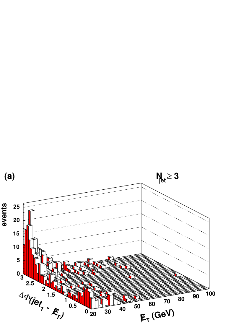
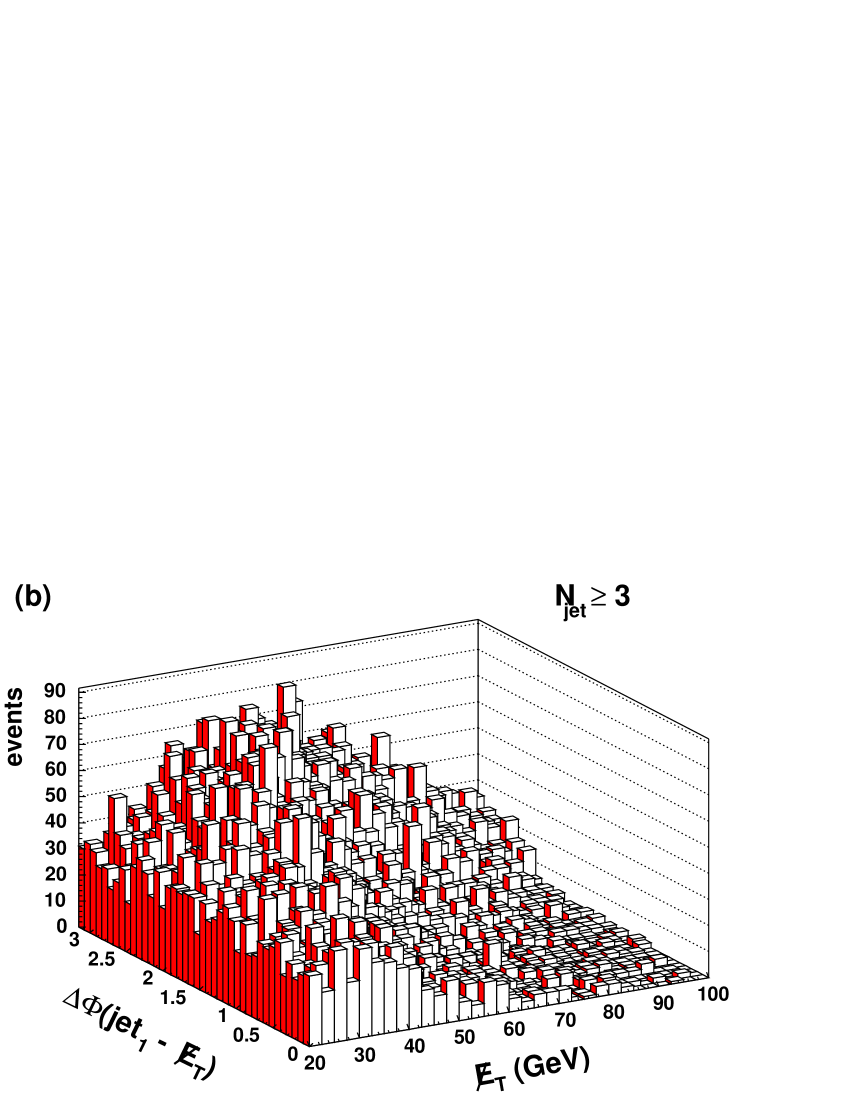
Figure 1: The angle in the transverse plane between the direction of the $\,/\!\!\!\!E_{T}$ and the leading jet versus the $\,/\!\!\!\!E_{T}$ for (a) our model of the multi-jet background from the non-isolated lepton data sample, and (b) PYTHIA ${t\bar{t}}$ Monte Carlo.

Backgrounds from processes with two or more high $p_{T}$ leptons include single top production and $Z$ boson, $WW$, $WZ$ and $ZZ$ diboson production with associated jets. We remove all events with two or more leptons satisfying the usual identification criteria in Tables 1 and 2. To avoid overlap with the ${t\bar{t}}$ dilepton analysis ttbardilepton , we also remove events that contain an additional lepton identified either as an electron in the plug calorimeter or as a muon with a track segment in CMU but outside the fiducial volume of CMP and vice versa. To further reduce the residual background from processes with leptonic $Z$ decays, we remove events where the primary lepton and a second object form an invariant mass within the 76-106  GeV/$c^{2}$ window containing the $Z$ boson mass. The criteria for this second object are designed to remove events where the second lepton is outside the fiducial volume of a calorimeter tower or muon chamber:

• The second object may be a lepton with relaxed identification requirements as listed in Table 4.

• The second object may be an isolated oppositely charged particle track with $p_{T}\geq 10$ GeV/$c$ that extrapolates back to within 10 cm of the z position of the event. In this case, isolated means that any additional tracks within a cone of radius $R=0.4$ have transverse momentum sum below 4.0 GeV/$c$.

• If the primary lepton is an electron, the second object may also be a jet with $E_{T}\geq 15$ GeV, $|\eta|\leq 2.0$, less than three tracks inside a cone of radius $R=0.4$, and over 95% of the total energy in the electromagnetic calorimeter.

The multi-lepton veto removes about 90% of $Z\rightarrow e^{+}e^{-}$ events and about 50% of $Z\rightarrow\mu^{+}\mu^{-}$ events, where the difference is due to the larger geometrical coverage of the calorimeter for electrons compared to that of the tracking system for muons. This multi-lepton veto is 96% efficient for ${t\bar{t}}$ events passing the previous requirements.

Table 4: Selection requirements for second lepton used in the $Z$ boson veto.

Property	Requirement
Electron
$E_{T}$	$\geq$ 10.0 GeV
$E_{\textrm{h}ad}/E_{\textrm{e}m}$	$\leq$ 0.12
Isolation	$\leq$ 0.15
Muon with a track segment in the muon chambers
$p_{T}$	$\geq$ 10.0 GeV/$c$
$E_{\textrm{h}ad}$	$\leq$ 10.0 GeV
$E_{\textrm{e}m}$	$\leq$ 5.0 GeV
$|\Delta x|$	$\leq$ 10.0 cm
$|d_{0}|$	$\leq$ 0.5 cm
Isolation	$\leq$ 0.15
Muon without a track segment in the muon chambers
$p_{T}$	$\geq$ 10.0 GeV/$c$
$E_{\textrm{h}ad}$	$\leq$ 6.0 GeV
$E_{\textrm{e}m}$	$\leq$ 2.0 GeV
$E_{\textrm{e}m}+E_{\textrm{h}ad}$	$\leq$ 10.0 GeV
$|d_{0}|$	$\leq$ 0.5 cm
Isolation	$\leq$ 0.15

III.9 Observed data events

In summary, our selection of ${t\bar{t}}\rightarrow\ell\bar{\nu_{\ell}}q\bar{q^{\prime}}b\bar{b}$ decays requires a $W\to\ell\nu$ candidate and at least three jets, which we will refer to as $W+\geq 3$jets. The $W$ boson candidate is one isolated lepton with $E_{T}\geq 20$ GeV and missing transverse energy $\,/\!\!\!\!E_{T}\geq 20$ GeV. Jets are reconstructed with a cone algorithm of radius $R=0.4$ and are required to have $E_{T}\geq 15$ GeV and $|\eta|<2.0$. In order to reduce the background from multi-jet processes, we require the directions of the $\,/\!\!\!\!E_{T}$ and the most energetic jet to be well-separated in the transverse plane if $\,/\!\!\!\!E_{T}<30$ GeV.

Table 5 lists the number of observed events in 194 pb^-1 of data, for the electron and muon channels separately and combined, as a function of the jet multiplicity. We also show our expectation for the number of ${t\bar{t}}$ events, where we use our estimate from the next section of the acceptance for a top mass of 175 GeV/$c^{2}$ and assume the NLO production cross section of 6.7 pb mlm ; kidonakis .

Table 5: The observed number of $W\to\ell\nu$ candidates as a function of the jet multiplicity, compared to the expectation from PYTHIA ${t\bar{t}}$ Monte Carlo simulation, where we assume a top mass of 175 GeV/$c^{2}$. We require at least 3 jets.

Jet multiplicity	Electron	Muon	Total	Expected ${t\bar{t}}$
0	99454	76203	175657	0.2
1	9407	6982	16389	4.4
2	1442	1054	2496	22.6
3	254	147	401	42.3
$\geq$ 4	78	40	118	49.9

IV Signal Acceptance

We measure the fraction of ${t\bar{t}}$ events accepted by our event selection requirements using a combination of Monte Carlo simulation and data. We generate ${t\bar{t}}$ events with the PYTHIA Monte Carlo program, which has a leading order matrix element for the parton hard scattering convoluted with the CTEQ5L parton distribution functions CTEQ . The acceptances from PYTHIA for each type of identified lepton are shown in the top line of Table 6. We correct these raw fractions for several effects, described in the previous section, that are not sufficiently well-modeled in our simulation: the lepton trigger efficiencies, measured from data; the fraction of the $p\bar{p}$ luminous region well-contained in the CDF detector, measured from data; the difference between the track reconstruction efficiency measured in data and simulation; and the difference between lepton identification efficiencies measured in $Z\rightarrow\ell^{+}\ell^{-}$ data and PYTHIA Monte Carlo. All of the correction factors for each type of identified lepton are shown in Table 6.

The total acceptance of our event selection for ${t\bar{t}}$ is $7.11\pm 0.56$%, given by the sum of the corrected acceptance weighted by the integrated luminosity of the data sample for each type of identified lepton. The uncertainty includes the systematic uncertainties discussed later in Section VIII. We assume a top mass of 175 GeV/$c^{2}$ and the PYTHIA branching fraction for $W\rightarrow\ell\nu$ of 10.8%. The acceptance is mostly from the ${t\bar{t}}\rightarrow\ell\nu q\bar{q}b\bar{b}$ channel, but also contains small contributions from other ${t\bar{t}}$ decay modes, as shown in Table 7.

Table 6: ${t\bar{t}}$ acceptance and correction factors. We assume a top mass of 175 GeV/$c^{2}$.

Quantity	CEM Electron	CMU/CMP Muon	CMX Muon
PYTHIA acceptance	0.0462 $\pm$ 0.0004	0.0283 $\pm$ 0.0003	0.0104 $\pm$ 0.002
Efficiency: Trigger	0.962 $\pm$ 0.006	0.887 $\pm$ 0.007	0.954 $\pm$ 0.004
Efficiency: Luminous region	0.948 $\pm$ 0.003	0.948 $\pm$ 0.003	0.948 $\pm$ 0.003
Correction: Track reconstruction	1.009 $\pm$ 0.002	1.009 $\pm$ 0.002	1.009 $\pm$ 0.002
Correction: Lepton identification	0.965 $\pm$ 0.014	0.887 $\pm$ 0.014	1.001 $\pm$ 0.017
Corrected acceptance	0.0412 $\pm$ 0.0033	0.0213 $\pm$ 0.0017	0.0095 $\pm$ 0.0008
Integrated luminosity (pb-1)	194	194	175

Table 7: Expected composition of selected ${t\bar{t}}$ events in terms of the various ${t\bar{t}}$ decay modes, as determined from PYTHIA ${t\bar{t}}$ Monte Carlo simulation.

${t\bar{t}}$ decay mode	Signal composition(%)
${t\bar{t}}\rightarrow\ell\nu q\bar{q}b\bar{b}$	82
${t\bar{t}}\rightarrow\tau\nu\ell\nu b\bar{b}$	7
${t\bar{t}}\rightarrow\tau\nu q\bar{q}b\bar{b}$	6
${t\bar{t}}\rightarrow\ell\nu\ell\nu b\bar{b}$	5

V Backgrounds

A variety of non-${t\bar{t}}$ processes can also produce events that pass our $W+\geq$3 jets selection requirements. These backgrounds can be grouped into three categories: production of a $W$ boson with associated jets, $W$+jets; other electroweak processes resulting in at least one high $p_{T}$ lepton and jets; and generic QCD multi-jet processes. However, theoretical predictions for the total rate of these processes only exist at leading-order, with associated uncertainties of 50% from the choice of scale used to evaluate the strong coupling constant $\alpha_{s}(Q^{2})$. Instead, we estimate their contribution to the data sample by exploiting the difference between the kinematics of these background processes and ${t\bar{t}}$ production. In this section, we discuss the Monte Carlo model we use to describe the kinematics of the $W$+jets and other electroweak processes. For the multi-jet events, we model their kinematics from an independent data sample and derive an estimate for their contribution.

Much theoretical progress has been made recently to improve the description of the kinematics of the $W$+jets process, with leading-order matrix-element generators now available to describe the parton hard scattering for processes with a $W$ boson and up to six well-separated partons in the final state. We use the ALPGEN ALPGEN matrix element generator, convoluted with the CTEQ5L parton distribution functions. We require parton $|\eta|\leq 3.0$, $p_{T}\geq 8$ GeV/$c$ and a minimum separation $\Delta R\geq 0.2$ between u, d, s and g partons at the generation level. We have verified that the shapes of the kinematic distributions used in our analysis are not sensitive to these values. We choose a default momentum transfer scale of $Q^{2}=M_{W}^{2}+\sum_{i}p_{T,i}^{2}$ for the parton distribution functions and the evaluation of $\alpha_{s}$, where $p_{T,i}$ is the transverse momentum of the $i$-th parton. We use the HERWIG parton shower algorithm to evolve the final state partons to colorless hadrons. Note that the addition of all of the $W$+n parton ALPGEN+HERWIG samples does not give a good model of the kinematics of the entire $W$+jets sample. For instance, for a given $W$+1 parton matrix element, the parton shower may radiate a gluon with large enough $p_{T}$ such that this final state would also be covered by the $W$+2 parton matrix element. We note that there has been significant recent theoretical and phenomenological progress here: an approach developed to solve this double-counting problem CKKW at $e^{+}e^{-}$ colliders has been adapted to the more complicated environment of hadron colliders and implemented in the PYTHIA and HERWIG Monte Carlo generators mrenna .

We use the $W$+n parton ALPGEN+HERWIG Monte Carlo to model the $W+\geq$n jet final state, where we rely on gluon radiation in the parton shower algorithm to adequately model the larger jet multiplicities. We also use the ALPGEN+HERWIG Monte Carlo to model $Z$ boson and diboson ($WW$, $WZ$, $ZZ$) production with associated jets. PYTHIA is used to simulate single top production. We show the composition of the background from electroweak processes in Table 8, where we use the leading order cross section from ALPGEN to normalize the contributions from different processes. We use the term “W-like” to refer collectively to all of these electroweak background processes.

Table 8: Expected composition of the $W$-like electroweak background in the electron and muon channels.

Process	Generator $\sigma$ (pb)	Electron (%)	Muon (%)
$W\rightarrow\ell\nu+$3 parton	179.8	87.3	84.8
$W\rightarrow\tau\nu+$3 parton	89.9	4.6	4.6
$Z\rightarrow\ell^{+}\ell^{-}+2$ parton	46.6	1.5	4.2
$Z\rightarrow\tau^{+}\tau^{-}+2$ parton	23.3	1.3	1.3
$WW$+1 parton	4.38	3.8	3.7
$WZ$+1 parton	2.37	0.4	0.4
single top	3.0	1.0	1.0

As discussed previously in Section III.8, multi-jet background events are often characterized by significant additional energy in the cone around the lepton and low missing transverse energy. We model the kinematics of the multi-jet background using data events that pass all of the selection requirements except for a lepton isolation requirement of $\geq$ 0.2. To estimate the rate of this background, we assume that there is no correlation between the $\,/\!\!\!\!E_{T}$ and the isolation of the identified lepton, shown in Fig. 2. The number of background events passing the selection requirements can then be estimated by comparing the number of events in various control regions:

• $n_{A}$: lepton isolation $I>0.2$ and $\,/\!\!\!\!E_{T}<10$ GeV

• $n_{B}$: lepton isolation $I<0.1$ and $\,/\!\!\!\!E_{T}<10$ GeV

• $n_{C}$: lepton isolation $I>0.2$ and $\,/\!\!\!\!E_{T}>20$ GeV.

Since the above numbers should reflect only the multi-jet process, corrections are made for the expected contribution from $W+$jets and ${t\bar{t}}$ events. In our signal region, defined by $\,/\!\!\!\!E_{T}>20$ GeV and lepton isolation $I<0.1$, the number of multi-jet events is estimated as $n_{C}\times n_{B}/n_{A}$. Table 9 lists the fraction of events in the signal region from QCD multi-jet processes as a function of jet multiplicity. We check the assumption of no correlation between $\,/\!\!\!\!E_{T}$ and isolation by variation of the requirements that define the control regions: this changes the estimates by $\pm$50%. We discuss the systematic uncertainty on this estimate further in Section VIII.

The larger multi-jet background in the electron data sample is partly due to electrons from unidentified photon conversions in detector material. The number of events identified by the photon conversion algorithm described in Section III.3 can be written as $N_{i}=\epsilon\times N_{c}+m\times(N+N_{i}-N_{c})$. The first term is the number of events with a photon conversion $N_{c}$ multiplied by the efficiency of the conversion algorithm, $\epsilon=72.6\pm 0.7\%$. The second term is the number of events without a photon conversion that are mis-identified by the conversion algorithm, where the mis-identification rate is $m=2.3\pm 0.04\%$ and $N$ is the number of events in the electron data sample. Therefore, the number of events remaining in the electron data sample with an unidentified photon conversion is $N_{u}=N_{c}\times(1-\epsilon)$. This estimate is shown in Table 10 and demonstrates that the majority of the QCD multi-jet background in the electron data sample comes from unidentified photon conversions.

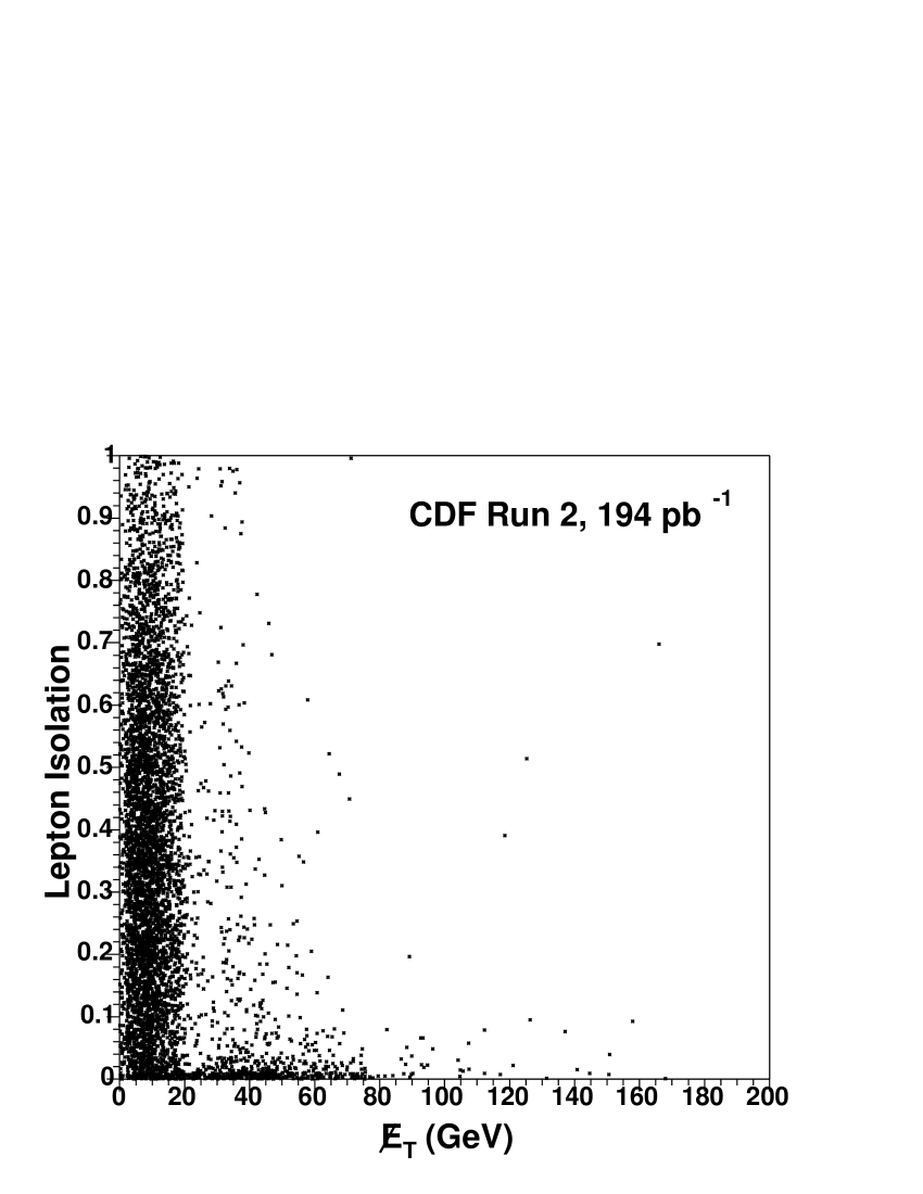
Figure 2: The $\,/\!\!\!\!E_{T}$ versus isolation distributions for events with a lepton and 3 or more jets. The structure apparent between 20 and 30 GeV comes from removing events where missing transverse energy lies close to the direction of the highest $E_{T}$ jet.

Table 9: The estimated fraction of the QCD multi-jet background in the $W$+jets data sample as a function of jet multiplicity. The uncertainty is statistical only.

Jet multiplicity	Electron	Muon	Total
1 jet	3.8 $\pm$ 0.2%	2.9 $\pm$ 0.2%	3.4 $\pm$ 0.3%
2 jets	6.1 $\pm$ 0.5%	2.0 $\pm$ 0.2%	4.3 $\pm$ 0.5%
$\geq$3 jets	7.7 $\pm$ 1.3%	3.1 $\pm$ 0.9%	6.3 $\pm$ 1.6%

Table 10: Estimate of the contribution to the electron data sample from unidentified conversions.

Jet	$N_{i}$	$N$	$N_{u}$	$N_{u}/N$
multiplicity	Identified conversion	Electron Data	Unidentified conversion	(%)
1 jet	791	9407	217 $\pm$ 13	2.3 $\pm$ 0.2%
2 jets	296	1442	100 $\pm$ 8	6.9 $\pm$ 0.5%
$\geq$3 jets	81	332	28 $\pm$ 4	8.4 $\pm$ 1.2%

VI Cross Section Measurement Method

A comparison of the observed number of data events with the expected number of signal for a ${t\bar{t}}$ cross section in the range predicted by theory is shown in Table 5. The sensitivity to top pair production from counting the observed number of events alone is overwhelmed by the 50% uncertainty on the leading-order theoretical prediction for the $W$+jets background. Previous CDF measurements of the top pair production cross section in the lepton+jets channel svxruniipaper have used $b$-tagging, at the cost of about 45% loss in signal acceptance, in order to improve the signal-to-background ratio and also use the more accurate prediction for the fraction of $W$+jets containing heavy flavor, where the leading-order scale dependence of the absolute cross sections largely cancels.

This analysis instead exploits the discrimination available from kinematic and topological properties to distinguish ${t\bar{t}}$ from background processes. Due to the large mass of the top quark, top pair production is associated with central, spherical events with large total $E_{T}$, unlike most of the background processes. We model the kinematics of ${t\bar{t}}$ and $W$-like background processes with Monte Carlo simulation. For the QCD multi-jet background, we model the kinematics with a non-isolated lepton data sample. We use these models to describe the data distribution of a suitably discriminating property. We extract the most likely number of events from ${t\bar{t}}$ production, $\mu_{{t\bar{t}}}$, from a binned maximum likelihood fit:

$$L(\mu_{{t\bar{t}}},\mu_{w},\mu_{q})=\prod^{N_{bins}}_{i=1}\frac{e^{-\mu_{i}}\mu_{i}^{d_{i}}}{d_{i}!},$$ (1)

where $\mu_{{t\bar{t}}}$, $\mu_{w}$, $\mu_{q}$ are the parameters of the fit, representing Poisson means for the number of ${t\bar{t}}$, W-like, and multi-jet events in our data sample. The expected number of events in the $i$-th bin is $\mu_{i}=(\mu_{{t\bar{t}}}P_{{t\bar{t}},i}+\mu_{w}P_{w,i}+\mu_{q}P_{q,i})$, where $P_{{t\bar{t}},i}$, $P_{w,i}$, $P_{q,i}$ is the probability for observing an event in the $i$-th bin from ${t\bar{t}}$, W-like and multi-jet processes respectively. The variable $d_{i}$ is the number of observed data events that populate the $i$-th bin. The number of multi-jet background events, $\mu_{q}$, is fixed to that expected from Table 9. Note that the uncertainty on our estimate of the number of multi-jet background events is included in the systematic uncertainties discussed in Section VIII.

We convert the fitted number of ${t\bar{t}}$ events into the top pair production cross section, $\sigma_{{t\bar{t}}}$, using the acceptance estimate, $\epsilon_{{t\bar{t}}}$, from Section IV, including the branching ratio for $W\rightarrow\ell\nu$, and the luminosity measurement $\mathcal{L}$:

$$\sigma_{{t\bar{t}}}=\frac{\mu_{{t\bar{t}}}}{\epsilon_{{t\bar{t}}}\mathcal{L}}.$$ (2)

In the rest of this section, we first describe our choice of a single kinematic discriminant, then how we maximize our discriminating power by developing an optimal variable with an Artificial Neural Network (ANN) technique. ANN’s employ information from several properties while accounting for the correlations among them NN .

VI.1 Single discriminant

We consider here a set of twenty properties, defined in Table 11, that provide good discrimination between signal and background. Fig. 3 compares the distributions from PYTHIA ${t\bar{t}}$ and ALPGEN+HERWIG $W+3$ parton Monte Carlo for each property. In the calculation of aplanarity and sphericity, we calculate the eigenvalues $Q_{i}$ of the normalized momentum tensor of the event, defined as $\frac{\sum_{i}{p_{i}^{a}p_{i}^{b}}}{{\sum_{i}{p_{i}^{2}}}}$ where the $a,b$ indices run over the three spatial directions and the summation is taken over the five highest $E_{T}$ jets, the lepton and the missing transverse energy. The variable $M_{W}^{\textrm{rec}}$ is intended to reconstruct the invariant mass of the jets from the $W\to jj$ decay. As we do not correct jets back to parton level, our simulation predicts that jets from the $W$ decay will have an invariant mass close to 66 GeV/$c^{2}$. Therefore, we pick the invariant mass of the two jets amongst the three highest $E_{T}$ jets that is closest to this value.

Table 11: The definition for all the kinematic and topological properties considered in this analysis.

Property	Definition
$H_{T}$	Scalar sum of transverse energies of jets, lepton and $\,/\!\!\!\!E_{T}$
Aplanarity	$3/2Q_{1}$
$\sum p_{z}/\sum E_{T}$	Ratio of total jet longitudinal momenta to total jet transverse energy
min($M_{jj}$)	Minimum di-jet invariant mass of three highest $E_{T}$ jets
$\eta_{max}$	Maximum $\eta$ of three highest $E_{T}$ jets
$\sum_{i=3}^{n}E_{T,i}$	Sum $E_{T}$ of third highest $E_{T}$ jet and any lower $E_{T}$ jets
min($\Delta R_{jj}$)	Minimum di-jet separation in $\eta$ and $\phi$ for three highest $E_{T}$ jets
$\sum_{i=1}^{n}E_{T,i}$	Sum $E_{T}$ of jets
$\,/\!\!\!\!E_{T}$	Missing transverse energy
Sphericity	$3/2(Q_{1}+Q_{2})$
$M_{event}$	Invariant mass of jets, lepton and $\,/\!\!\!\!E_{T}$
$M_{12}+M_{23}+M_{13}$	Sum of di-jet invariant masses of three highest $E_{T}$ jets
$E_{T}^{j1}$	$E_{T}$ of jet with highest $E_{T}$
$E_{T}^{j2}+E_{T}^{j3}$	Sum of $E_{T}$ of jets with second and third highest $E_{T}$
$M_{W}^{rec}$	Di-jet invariant mass closest to 66.0 GeV of three highest $E_{T}$ jets
$\sum_{i=1}^{3}\eta_{i}^{2}$	Sum of $\eta^{2}$ of three highest $E_{T}$ jets
$\Delta\Phi_{lm}$	Azimuthal angle between lepton and $\,/\!\!\!\!E_{T}$
$E_{T}^{j2}$	$E_{T}$ of jet with second highest $E_{T}$
$E_{T}^{j3}$	$E_{T}$ of jet with third highest $E_{T}$
$E_{T}^{j1}+E_{T}^{j2}$	Sum of $E_{T}$ of jets with first and second highest $E_{T}$

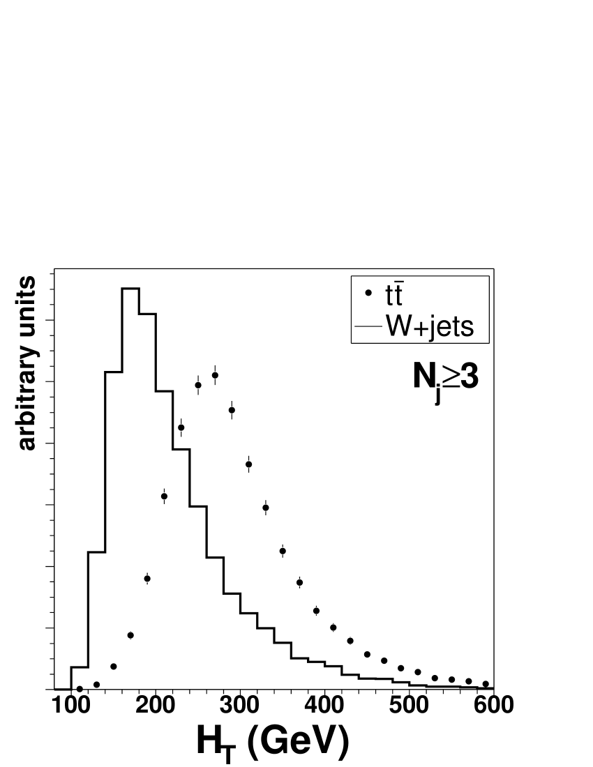
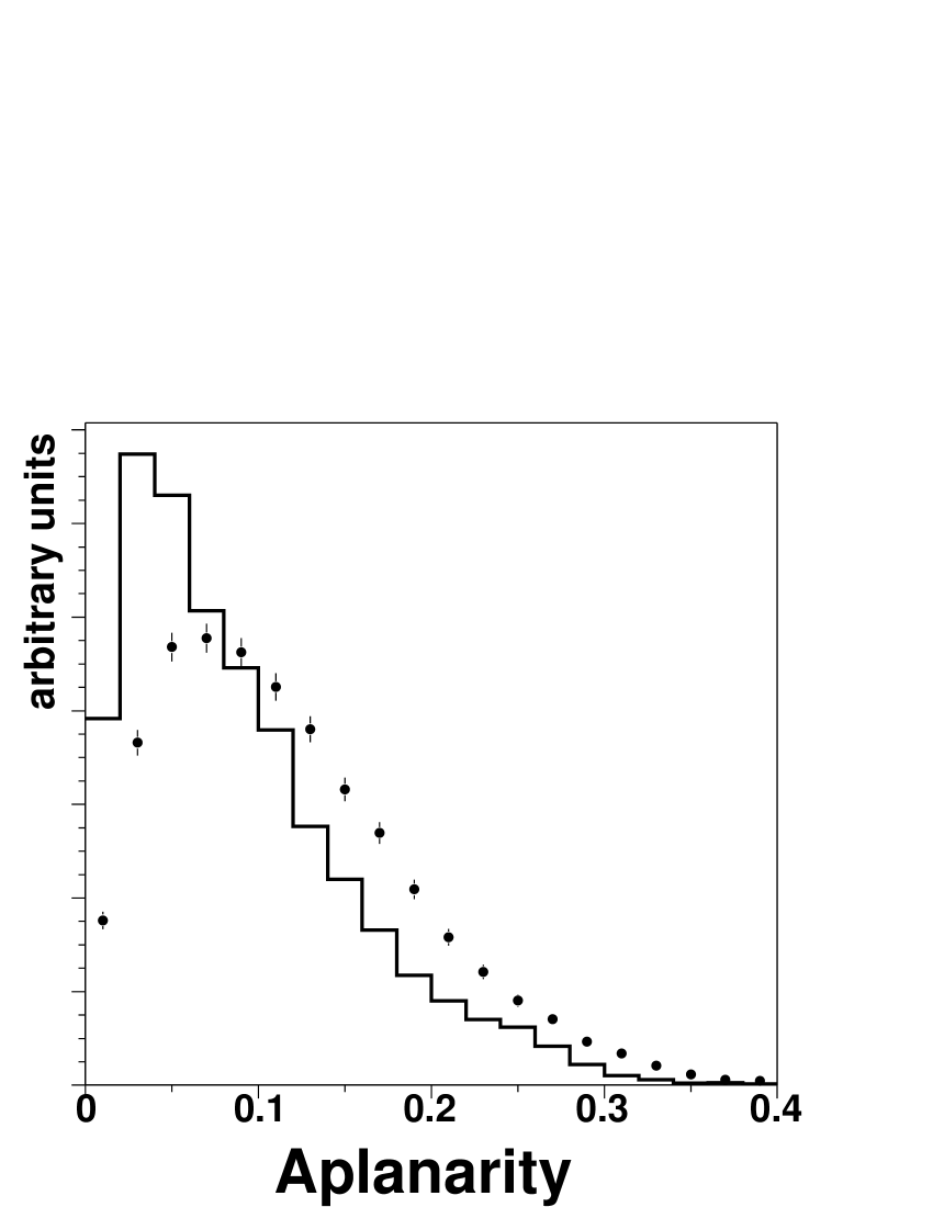
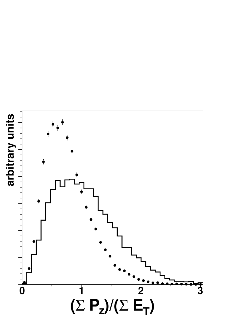
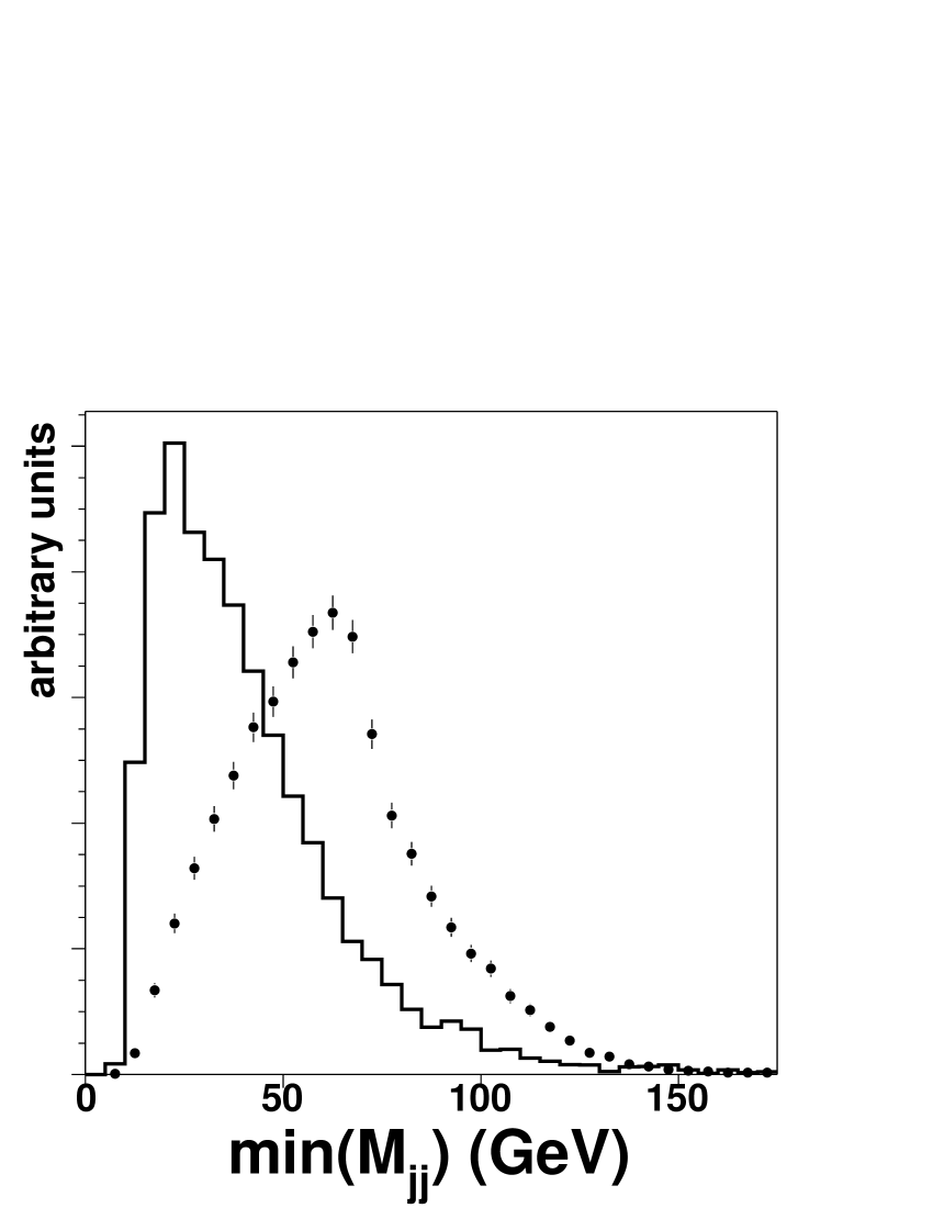
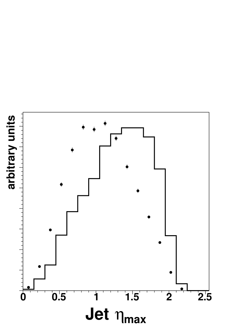
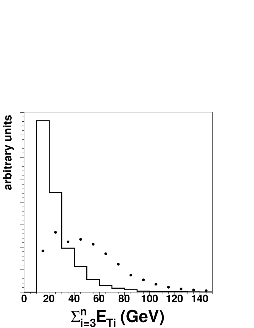
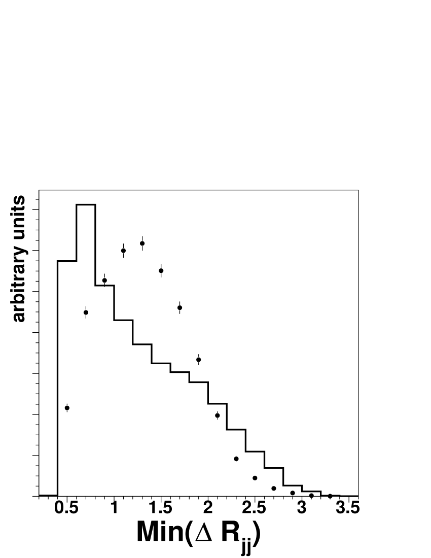
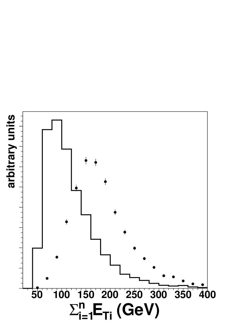
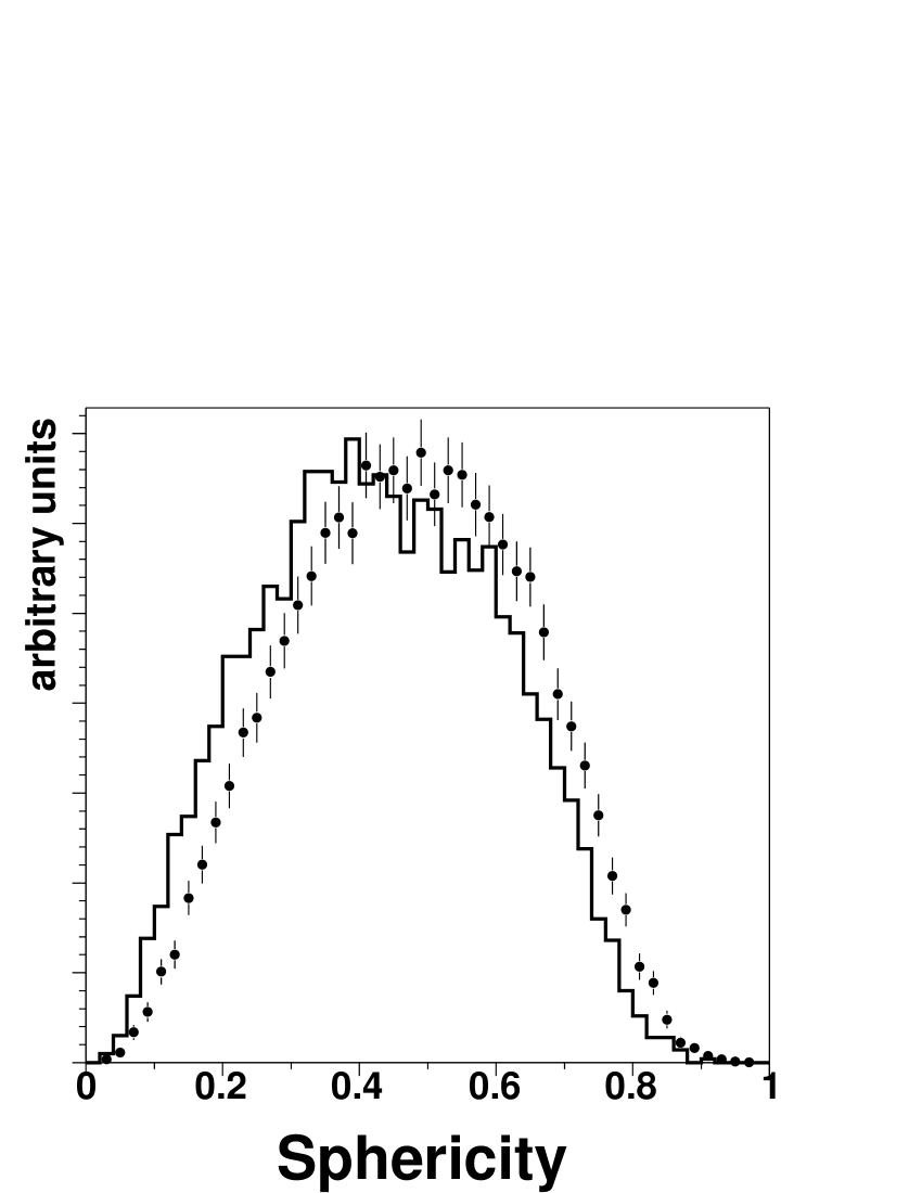
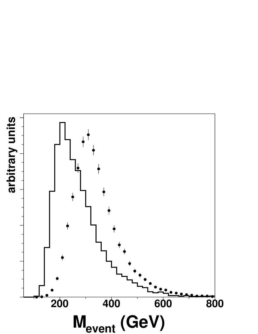
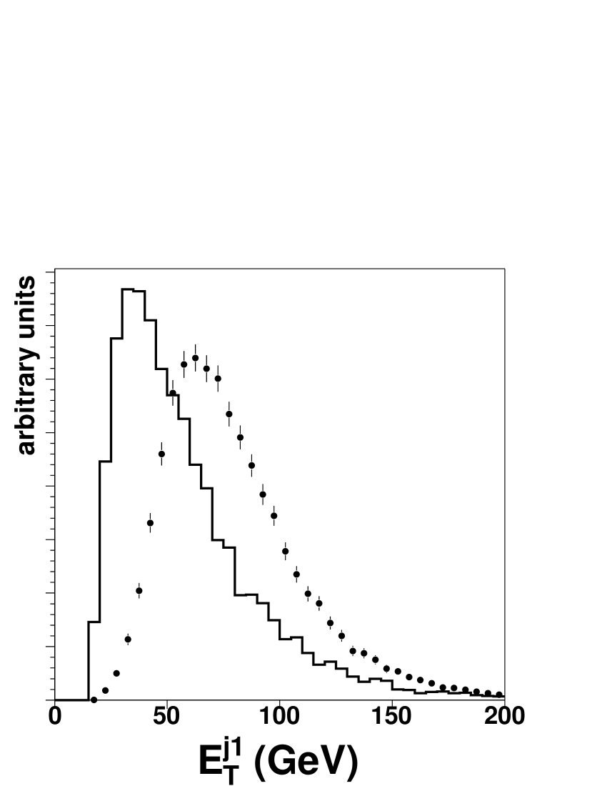
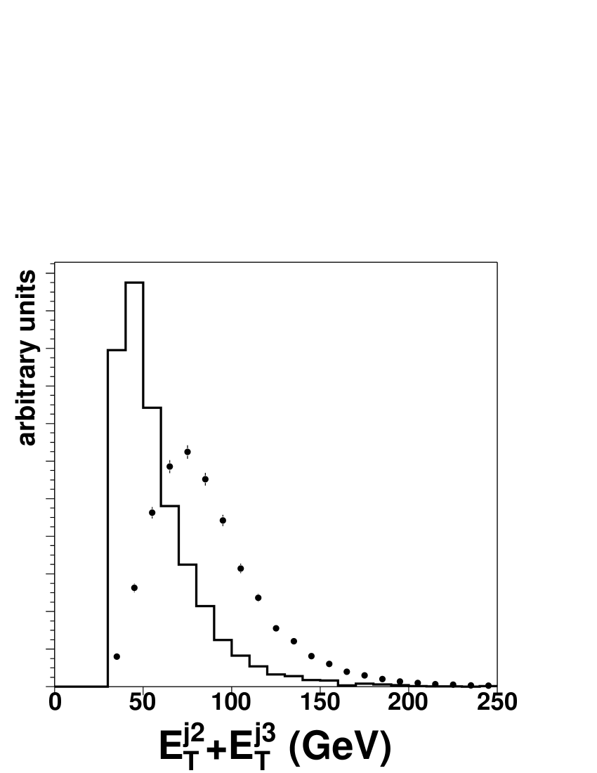
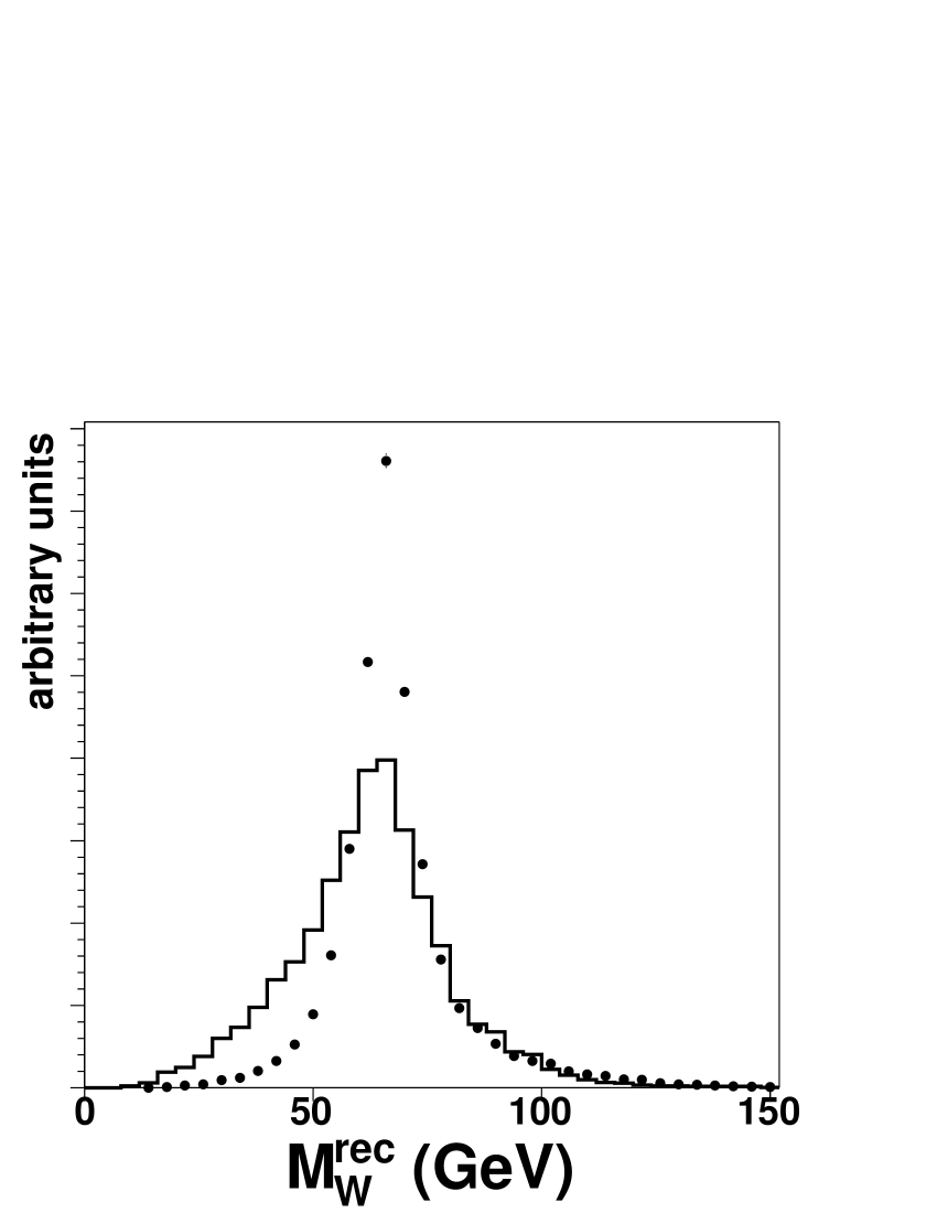
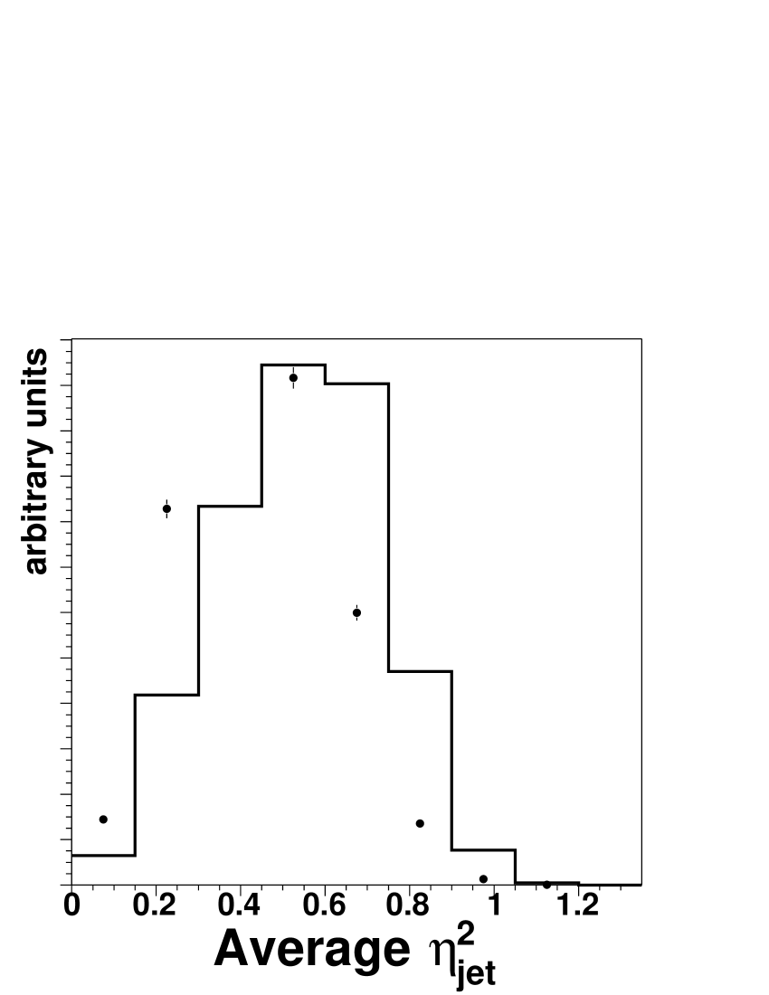
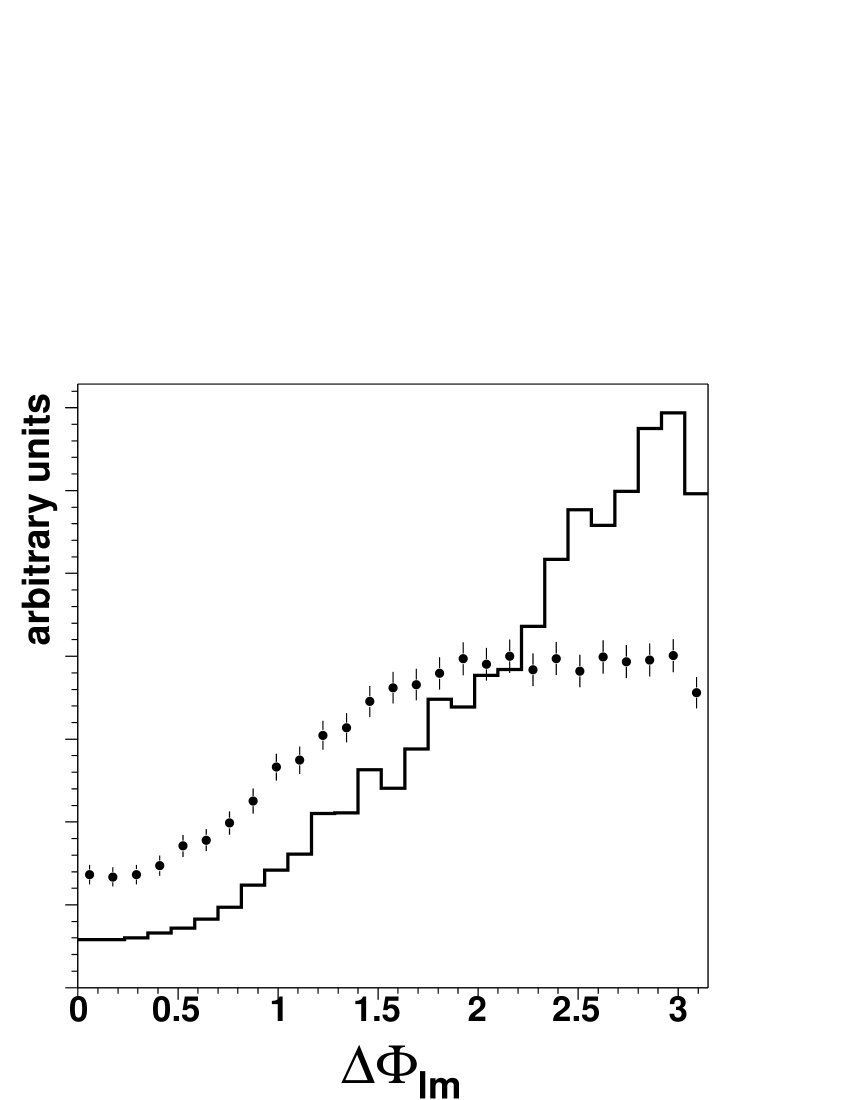
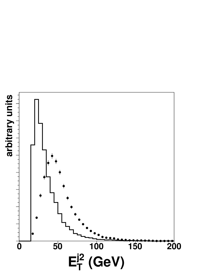
Figure 3: Shape comparison of PYTHIA ${t\bar{t}}$ to ALPGEN +HERWIG $W$+3p Monte Carlo simulation for the twenty kinematic and topological properties considered for the $W+\geq$3 jets sample. The distributions are normalized to equal area.

The expected statistical sensitivity of each single property is estimated a priori by constructing simulated experiments of the same size on average as the data sample from Table 5. Each simulated experiment contains $N_{{t\bar{t}}}$ signal ${t\bar{t}}$ events drawn from a Poisson distribution with mean given by Table 5, $N_{q}$ multi-jet background events drawn from a Poisson distribution with mean given by Table 9, and $N_{w}$ W-like background events drawn from a Poisson distribution with mean equal to the remainder. In every simulated experiment, we perform a separate binned maximum likelihood fit for each of the twenty single properties. The expected statistical uncertainty on the number of ${t\bar{t}}$ events is shown in Fig. 4 for all twenty single properties in the $W+\geq$3 jets sample. A similar sensitivity plot for the $W+\geq$4 jets sample is shown in Fig. 5.

We choose to use the total transverse energy in the event, $H_{T}$, since it is both one of the observables that provides good discrimination between events containing top decays and events from background processes, and since it has been commonly used in other analyses for this purpose ttbardilepton ; svxruniipaper . We note that the sum of the jet transverse energies or the transverse energy of the third most energetic jet have similar statistical power. From a fit to the $H_{T}$ distribution in the $W+\geq$3 jets sample, we expect to obtain a statistical uncertainty in the range 19-29% for 68% of data-sized experiments, with a median at 23.5%.

Although the $W+\geq$4 jets sample has an improved signal to background ratio, we find a larger expected statistical uncertainty in the range 25-48% for 68% of data-sized experiments, with a median of 32%. The lower sensitivity is due to both lower statistics - 45% of the ${t\bar{t}}$ events fail the 4th jet requirement - and reduced discriminating power- the increased jet activity means that $W+\geq$4 jet events have larger $H_{T}$ and are therefore more similar to top pair production. Finally, we note that the systematic uncertainty, discussed in Section VIII, is also about 20% larger, in part due to the increased sensitivity of the selection to the jet energy scale.

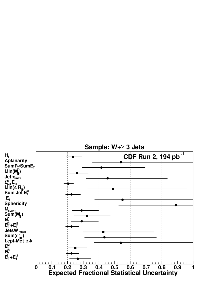
Figure 4: Expected statistical sensitivity of fits to each of the kinematic distributions for the $W+\geq$3 jets sample. The points mark the median of the relative error distribution, the error bars mark the 16-84 percentile interval.

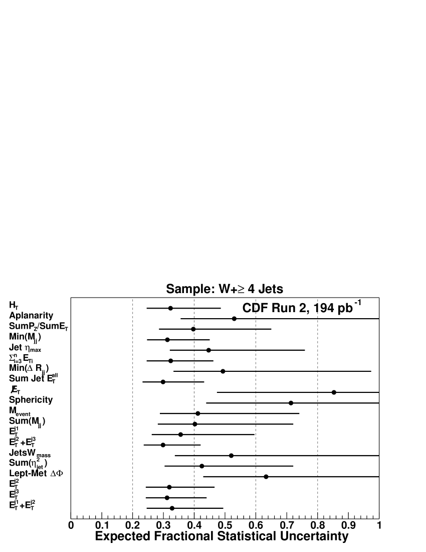
Figure 5: Expected statistical sensitivity of fits to each of the kinematic distributions for the $W+\geq$4 jets sample. The points mark the median of the relative error distribution, the errors bars mark the 16-84 percentile interval.

VI.2 Artificial Neural Network

The ANN that we develop is a feed-forward network perceptron with one intermediate (hidden) layer and one output node. Training of the network is performed with 4000 PYTHIA ${t\bar{t}}$ and 4000 $W$+3 parton ALPGEN+HERWIG Monte Carlo events that pass the selection requirements. During the iterative training, the weights of the network are adjusted in order to minimize a mean squared error function cata15 :

$$E=\frac{1}{N}\sum_{i=1}^{N}{(O_{i}-t_{i})^{2}}$$

where $N$ is the number of events in the training sample, $O_{i}$ is the output of the network and $t_{i}$ is the desired target value for the $i$-th event. We choose a target value of 1.0 for signal events and 0.0 for background events. We use the back-propagation training method from the JETNET jetnet software package, with a pruning option turned on that has the effect of adding a regularization term to the error function in order to discourage unnecessary weights. The iterative training is halted at the point where the error function has the lowest value on an independent sample of Monte Carlo simulated events. This protects the ANN from effects due to statistical fluctuations in the training sample.

For inputs to the ANN, we consider many different combinations of twenty kinematic and topological properties described in Table 11. The performance of each artificial neural network is tested a priori by constructing simulated experiments as before, where now we simply treat the output of the ANN as a single discriminant. We show that the addition of more inputs to the ANN reduces the expected statistical uncertainty in Fig. 6 and the average systematic uncertainty, described in Section VIII, in Fig. 7. In either case, there is little gain beyond seven inputs. For each increment in the number of inputs, one extra property is added in the order given in Table 11. The network with one input uses the kinematic property $H_{T}$. We note that this order is somewhat arbitrary, as there are other combinations that would give similar performance at each stage.

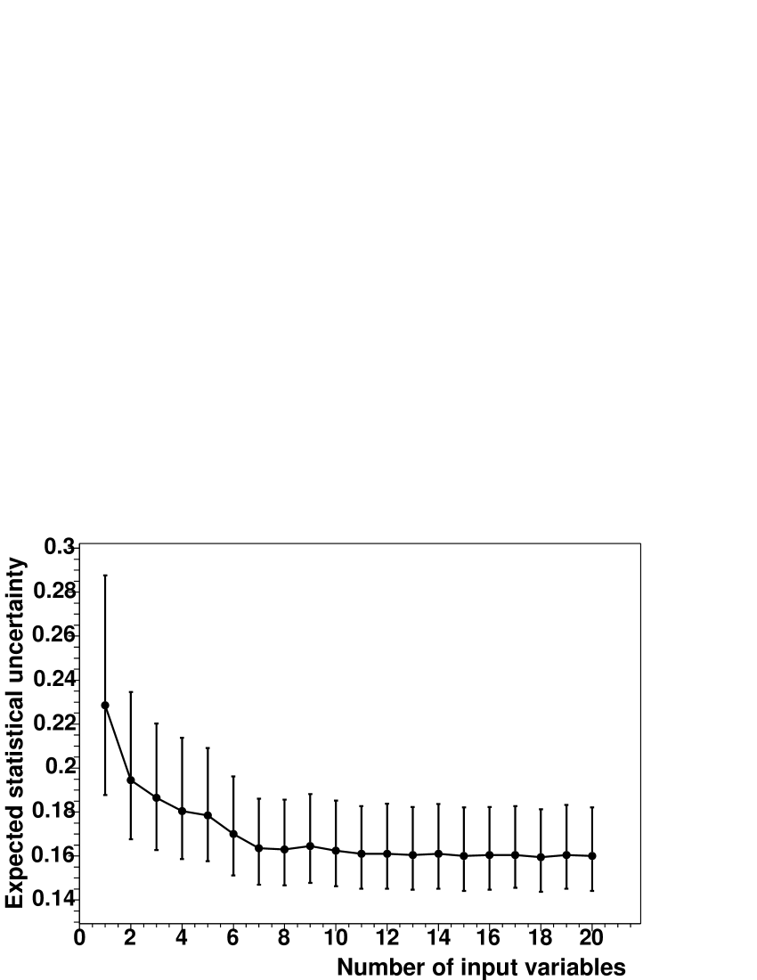
Figure 6: Expected statistical sensitivity for ANNs with the number of inputs ranging from 1-20 for the $W+\geq$3 jets sample. The points represent the median in the relative error distribution, error bars mark the 16-84 percentile interval.

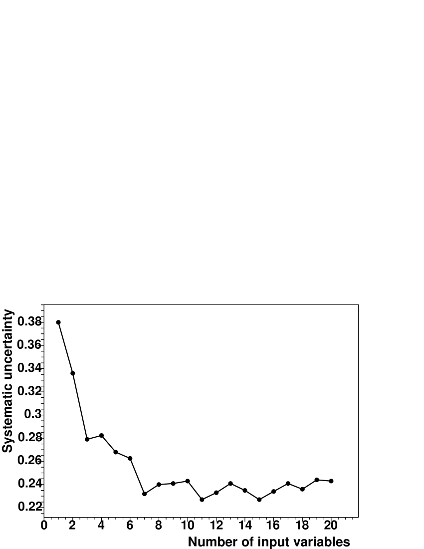
Figure 7: Average systematic uncertainties for ANNs with the number of inputs ranging from 1-20 for the $W+\geq$3 jets sample.

Although simplicity may not be a stringent requirement lessons , we choose a seven input network as the minimal configuration yielding good performance. The properties chosen are the first seven listed in Table 11: (1) the total transverse energy in the event $H_{T}$, (2) the event aplanarity, (3) the ratio between total jet longitudinal momenta and the total jet transverse energy, (4) the minimum di-jet invariant mass of the three highest $E_{T}$ jets, (5) the maximum jet rapidity of the three highest $E_{T}$ jets, (6) the sum of transverse energy of the third highest $E_{T}$ jet and any other lower $E_{T}$ jets, and (7) the minimum di-jet separation. For these seven input properties, we compare the average statistical and systematic uncertainties for ANNs with 1 to 10 nodes in the hidden layer. We choose a 7-7-1 ANN configuration, which consists of seven input properties, seven hidden nodes and one output unit. We expect to obtain a statistical uncertainty in the range 15-19% for 68% of data-sized experiments, with a median at 16.5%. This is a relative improvement of 30% with respect to the $H_{T}$ distribution alone.

For the $W+\geq$4 jet sample, which has higher signal to background ratio but lower signal acceptance, we train a second 7-7-1 ANN with the same seven input properties. We use $W$+4p ALPGEN+HERWIG Monte Carlo to model the kinematics of the background. We find a larger expected statistical uncertainty, in the range 19-28% for 68% of data-sized experiments, with a median of 23%. The lower sensitivity is due to both lower statistics - 45% of the ${t\bar{t}}$ events fail the 4th jet requirement - and reduced discriminating power- the increased jet activity means that $W+\geq$4 jet events are topologically and kinematically more similar to top pair production. Even so, we note that the sensitivity here is comparable to that from the single $H_{T}$ distribution in the $W+\geq$3 jet sample.

Finally, in order to check that our fit procedure is unbiased, we constructed simulated experiments with input ${t\bar{t}}$ signal cross sections ranging from 1 pb to 12 pb. In all cases, we find that the average measured ${t\bar{t}}$ cross section using the 7-7-1 ANN is consistent with the input ${t\bar{t}}$ cross section.

VII Check of Monte Carlo modeling

The method described in the previous section relies on the accurate modeling of kinematic and topological quantities by Monte Carlo generators and on the accurate description of the detector response by the simulation of the CDF detector. We compare kinematic and topological properties of the mutually exclusive $W$+1 jet, $W$+2 jet, and $W$+3 jet samples with our model. A Kolmogorov-Smirnov (KS) statistic is used to quantify the quality of the agreement.

In the $W+1$ and $W+2$ jet samples, we neglect the ${t\bar{t}}$ contribution as this is expected to be negligible, as shown in Table 5. Fig. 8 shows the leading jet $E_{T}$, $\,/\!\!\!\!E_{T}$ and $H_{T}$ distributions for $W+1$ jet and $W+2$ jet data events compared to the prediction from ALPGEN+HERWIG $W+1p$ and $W+2p$ Monte Carlo respectively, and our model of the QCD multi-jet background from non-isolated lepton data. We observe better agreement between data and our model in the $W$+2 jet sample than in the $W$+1 jet sample. As we noted in Section V, our $W+n$ parton model of the $W+\geq n$ jets background approximates the contributions from higher-order matrix elements with a parton shower, which does not alter the kinematics of the $W$ boson. This effect is most pronounced in the $W$+1 jet region, which has the largest relative change in the shape of the $W$ boson $p_{T}$ between $W$+n parton and $W$+(n+1) parton. With the larger statistics available in the 1 and 2-jet bins, the QCD multi-jet background is allowed to float and a two-component binned maximum likelihood fit is performed to the data.

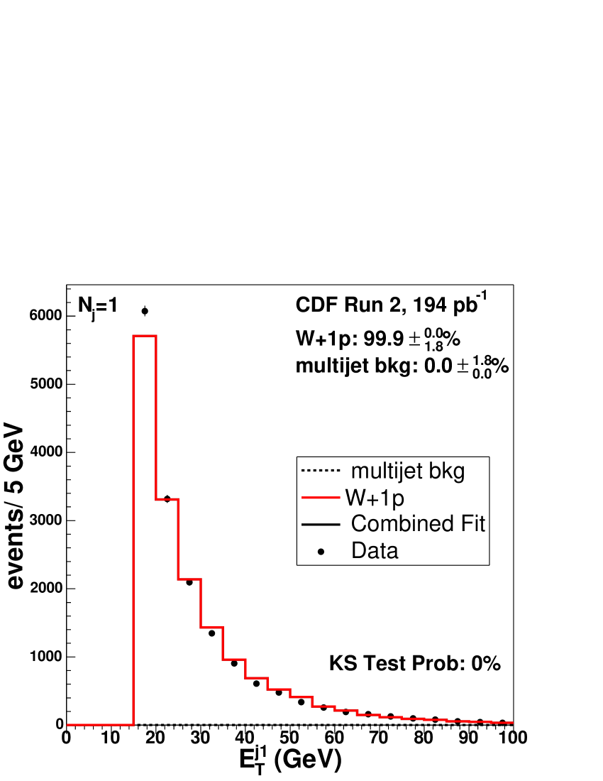
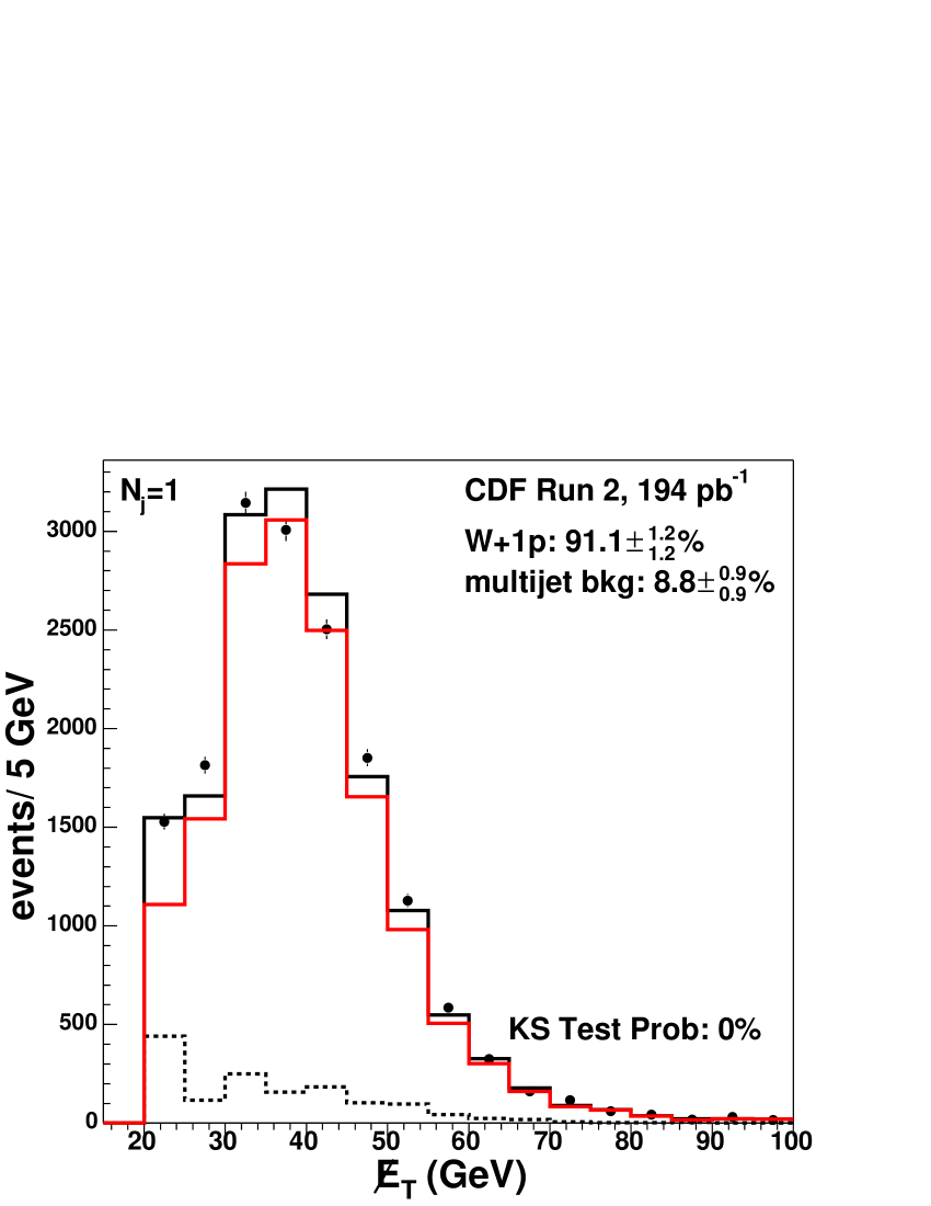
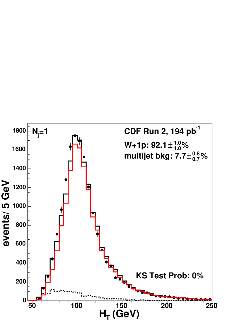
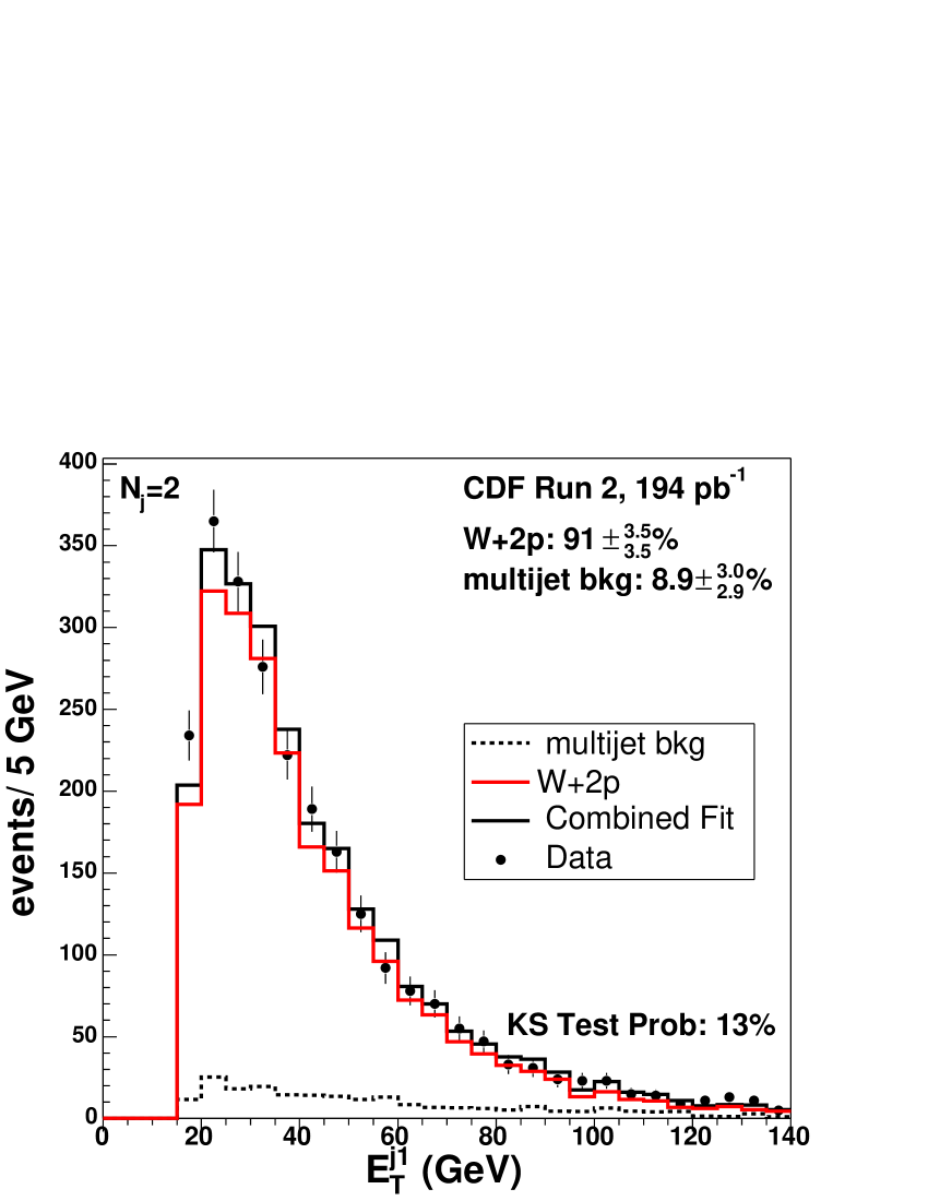
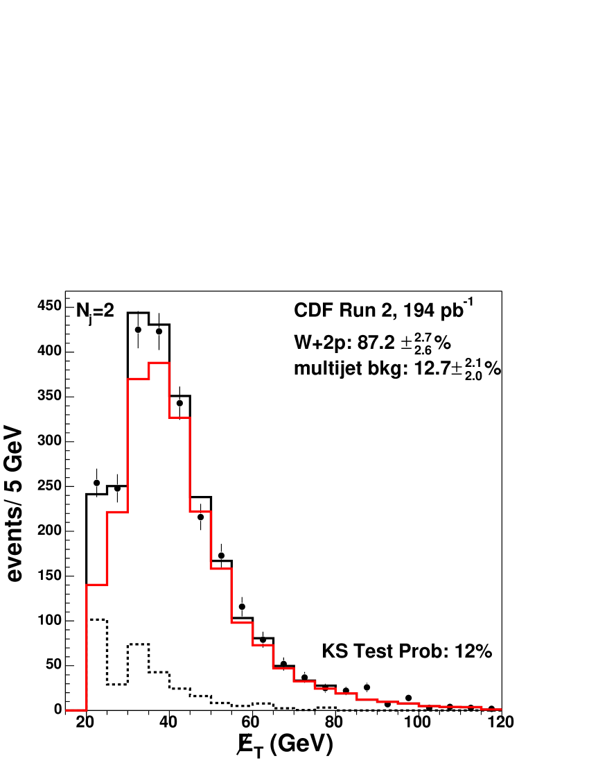
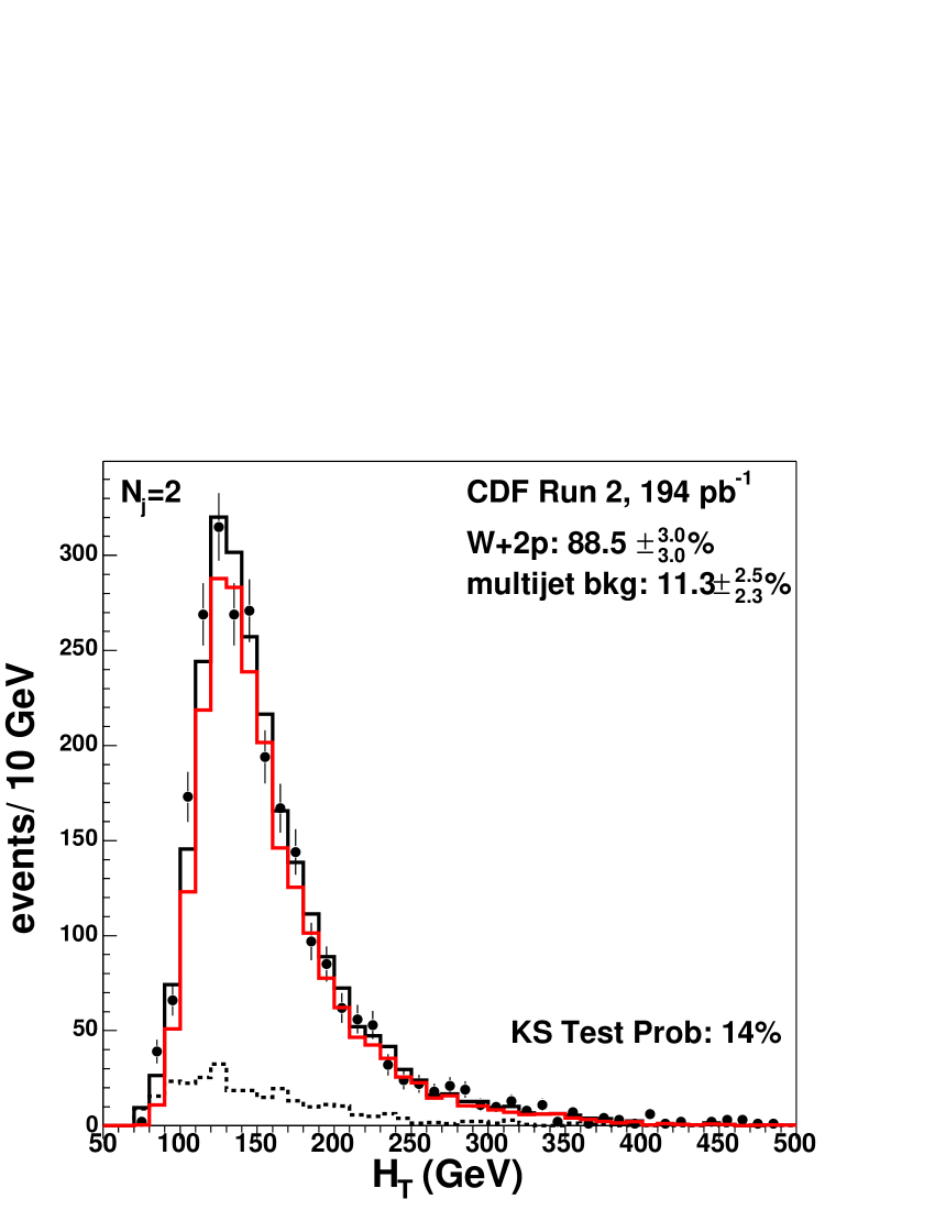
Figure 8: The leading jet $E_{T}$  $\,/\!\!\!\!E_{T}$, and $H_{T}$ distributions for $W+1$ and $W+2$ jet events compared to the prediction from ALPGEN+HERWIG $W+1p$ and $W+2p$ Monte Carlo and multi-jet background distributions. A binned maximum likelihood fit is performed to the data, allowing the number of QCD background events to fluctuate. Note that the $\,/\!\!\!\!E_{T}$ distribution is sculpted between 20 and 30 GeV by the multi-jet background rejection of Section III.8.

As discussed in the previous section, we use events with three or more jets for our ${t\bar{t}}$ cross section measurement. In the $W+3$ jet sample, we expect a contribution of only about 10% from ${t\bar{t}}$, as shown in Table 5. This latter region is top-depleted but otherwise kinematically and topologically identical to the majority of the background in the signal sample. Therefore we use events with exactly three jets to make a complete comparison of all the discriminating properties and the correlations between them. Fig. 9 shows the distributions for the leading jet $E_{T}$, $\,/\!\!\!\!E_{T}$, $H_{T}$, as well as other ANN input properties for $W+3$ exclusive jet events compared to the prediction from the ALPGEN+HERWIG $W$+3p Monte Carlo, multi-jet background and PYTHIA ${t\bar{t}}$ Monte Carlo. The model here is not the result of a binned maximum likelihood fit but rather has the ${t\bar{t}}$ fraction fixed to 10% as expected for a top mass of 175 GeV/$c^{2}$ in Table 5, the multi-jet background to the 6% estimate from Table 9, and the W+jets background as the remaining 84%. A similar comparison for the output of the ANN in the $W+3$ jet exclusive sample is shown in Fig. 10. Overall, the KS test values indicate good agreement between data and the Monte Carlo simulation.

The correlations between the various kinematic and topological properties also provide information that we use in our multivariate approach. We have looked at the pair correlations for the 7 input properties used in the ANN. For two generic variables $x$ and $y$, a correlation variable $corr(x,y)$ is defined on event by event basis:

$$corr(x,y)=\frac{(x-\overline{x})\cdot(y-\overline{y})}{(\Delta x\cdot\Delta y)^{1/2}},$$ (3)

where $\overline{x}$ is the average value in the $x$ variable and $\Delta x=\overline{(x-\overline{x})^{2}}$. Fig. 11 and Fig. 12 show the distributions for the event-by-event correlations between the 7 ANN input properties for $W+3$ exclusive jet events, compared to the predictions from the ALPGEN+HERWIG $W$+3p Monte Carlo and PYTHIA ${t\bar{t}}$ Monte Carlo. The model here is a combination of 10% ${t\bar{t}}$ and 90% W+jets simulated events. Overall, the KS test values indicate agreement between data and the Monte Carlo simulation.

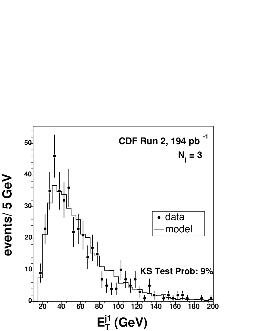
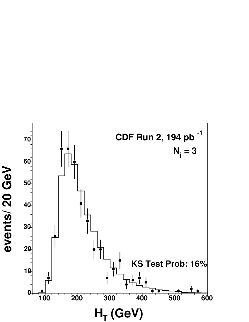
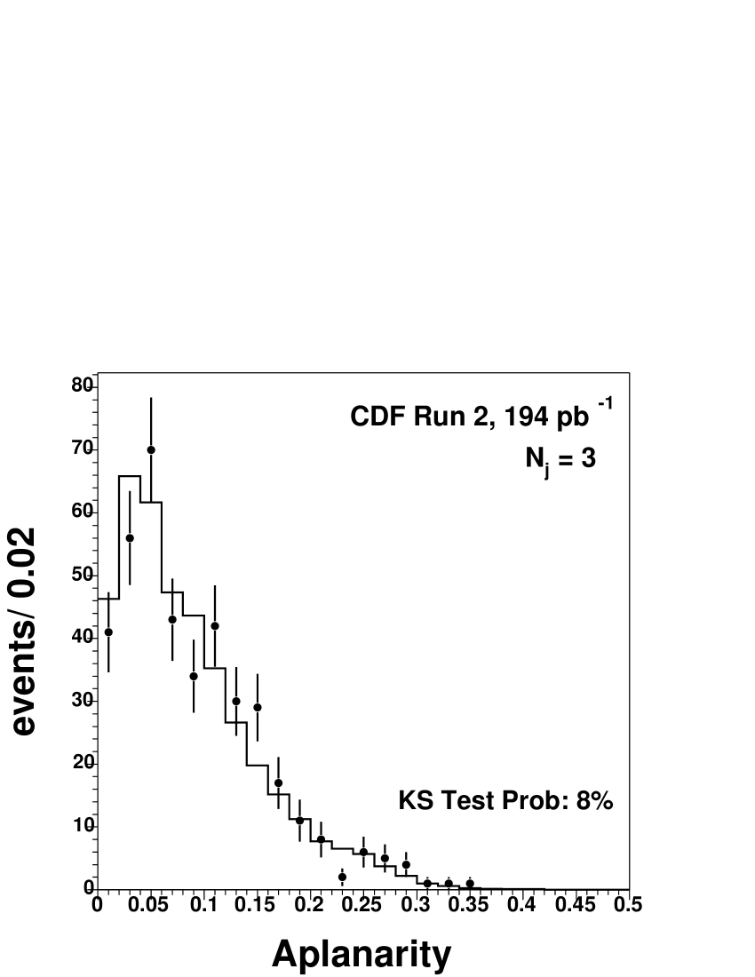
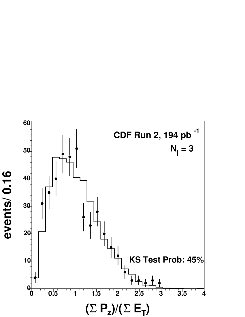
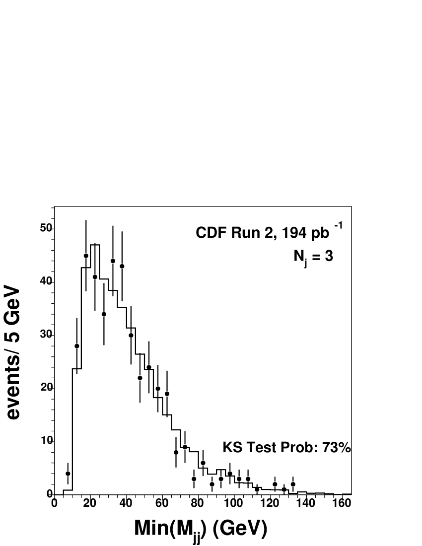
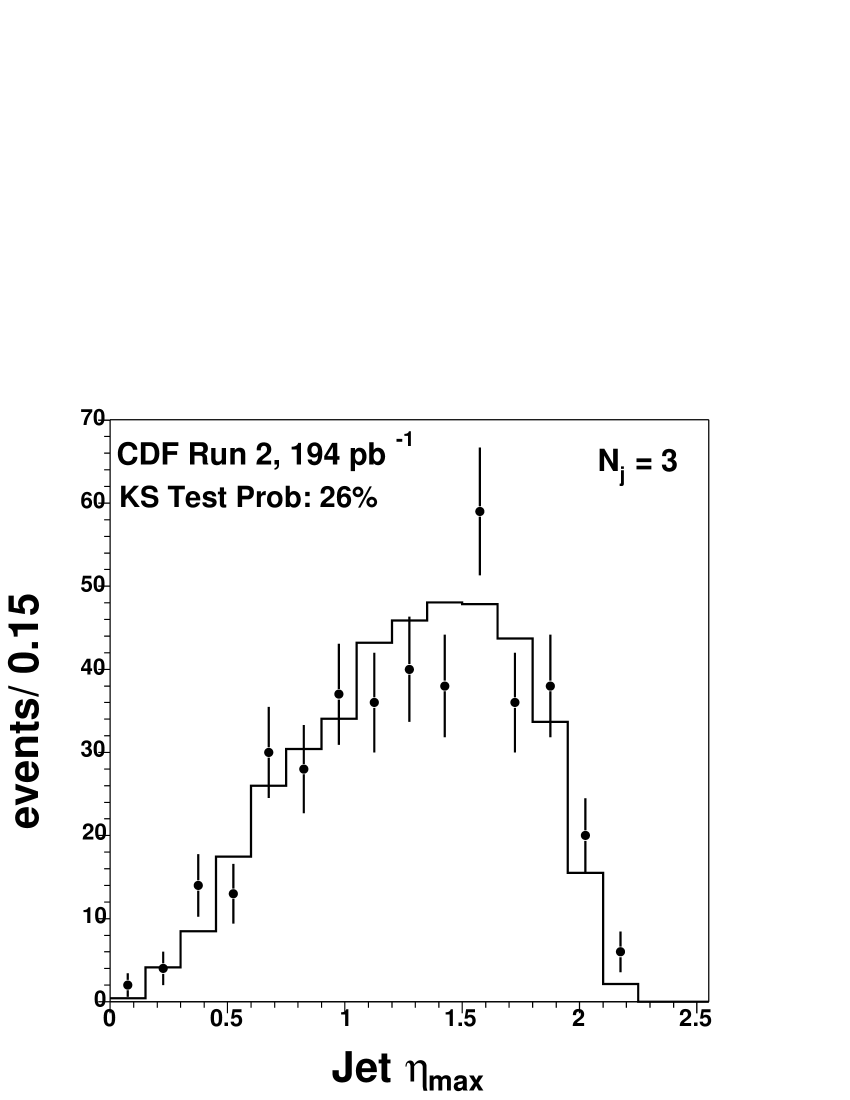
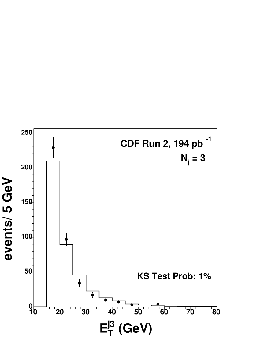
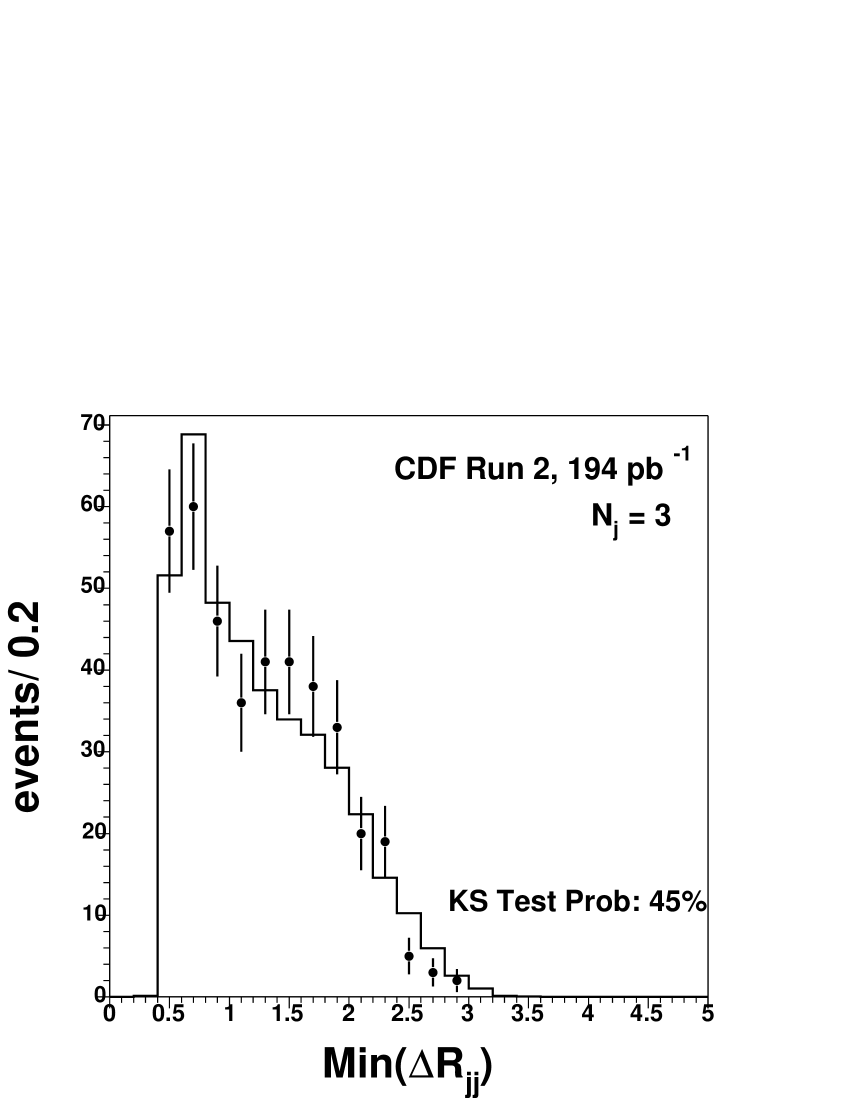
Figure 9: The $\,/\!\!\!\!E_{T}$, leading jet $E_{T}$, and the seven ANN input distributions in $W+3$ exclusive jet events compared to the predictions from ALPGEN+HERWIG $W$+3p Monte Carlo, multi-jet background,and PYTHIA ${t\bar{t}}$ Monte Carlo. The model here is a combination of 84% $W$+jets simulated events with 6% multi-jet background, and 10% ${t\bar{t}}$ simulated events.

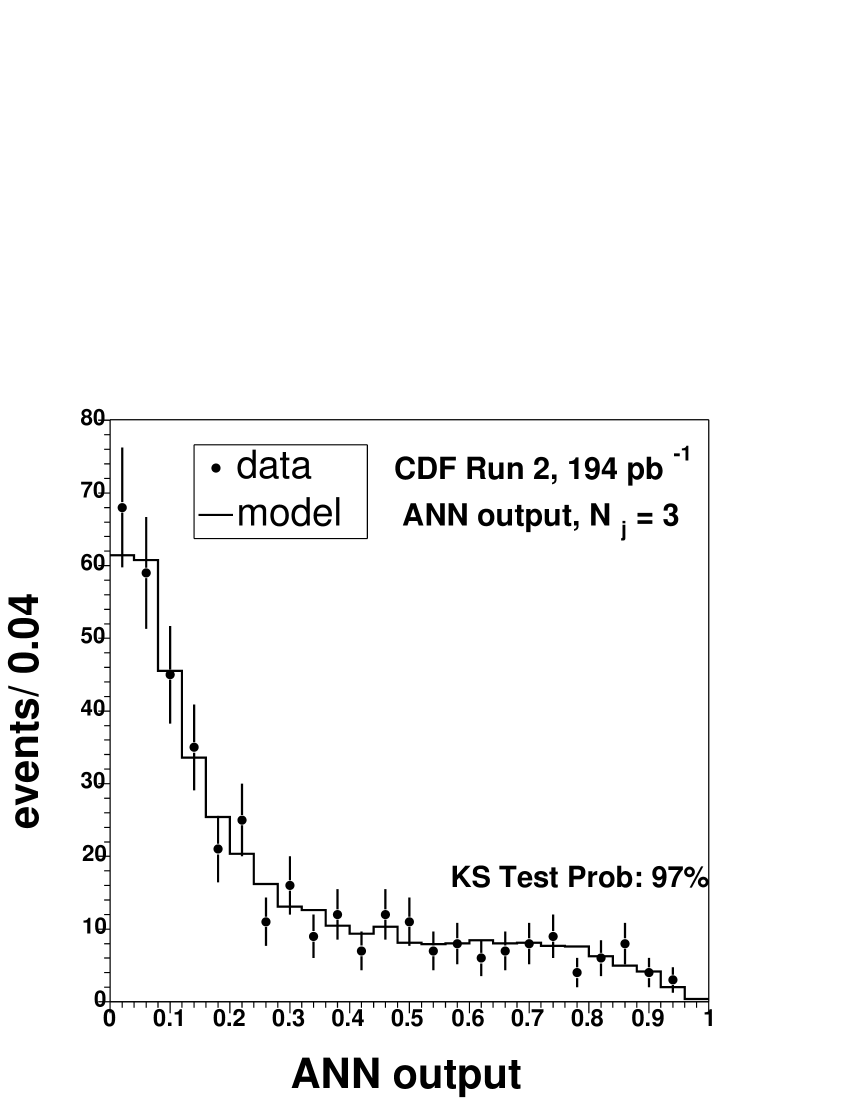
Figure 10: The distribution for the ANN output for $W+3$ exclusive jet events compared to the prediction from ALPGEN+HERWIG $W$+3p Monte Carlo, multi-jet background and PYTHIA ${t\bar{t}}$ Monte Carlo. The model here is a combination of 84% $W$+jets simulated events with 6% multi-jet background, and 10% ${t\bar{t}}$ simulated events.

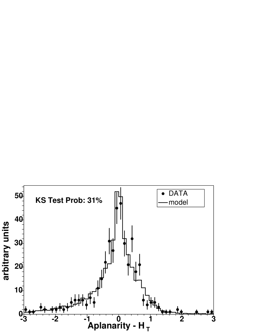
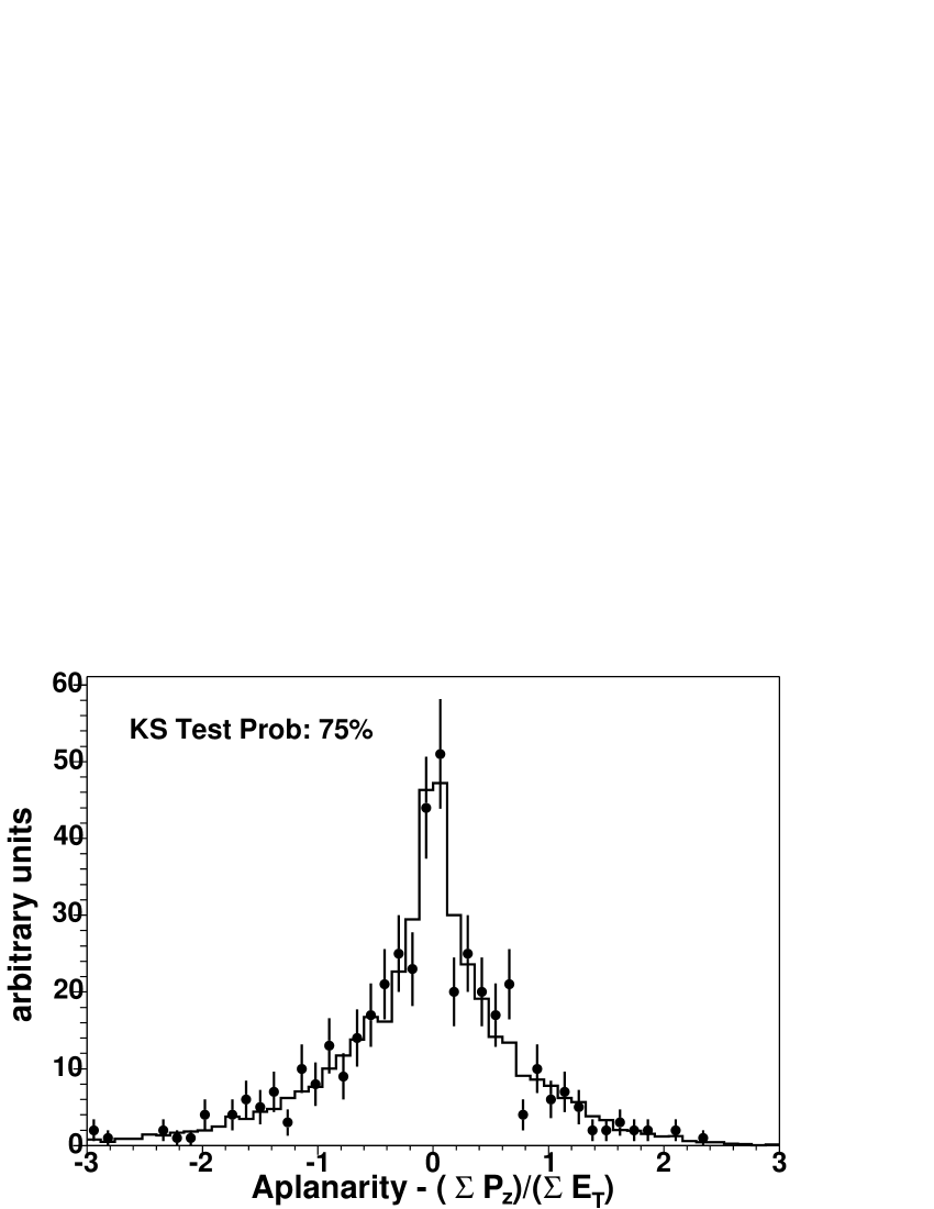
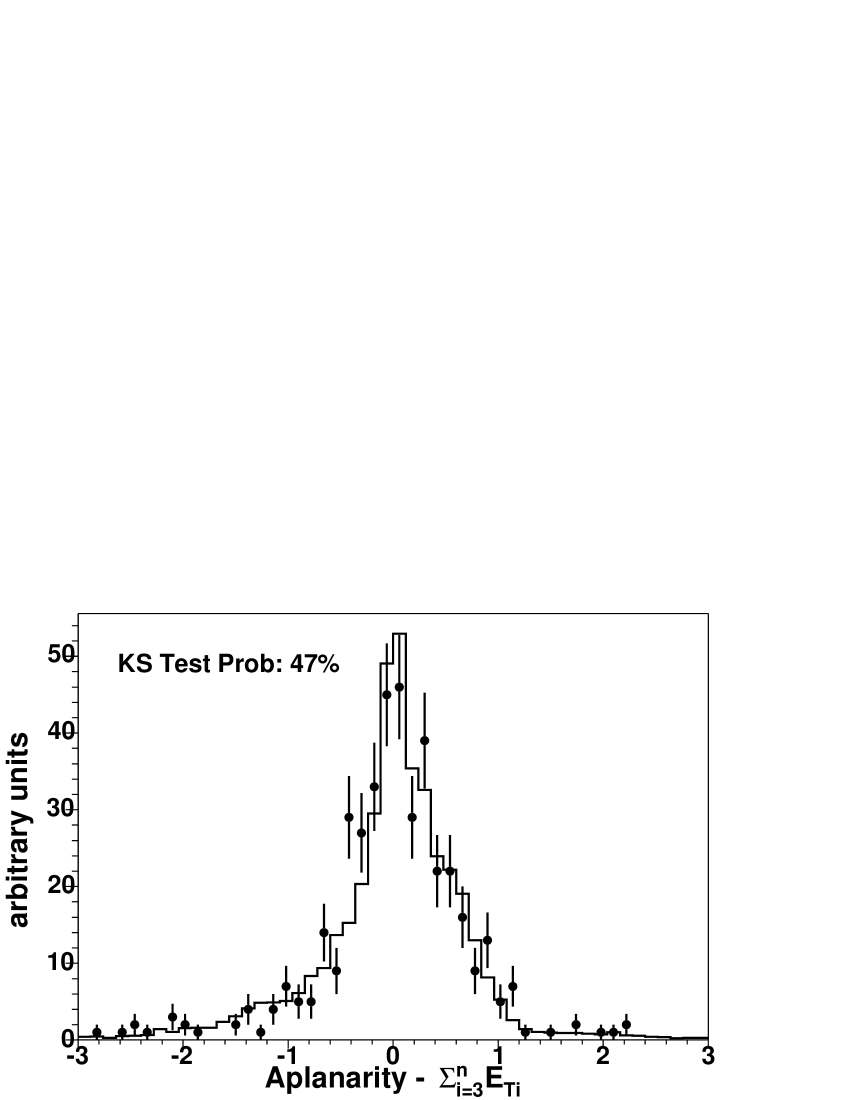
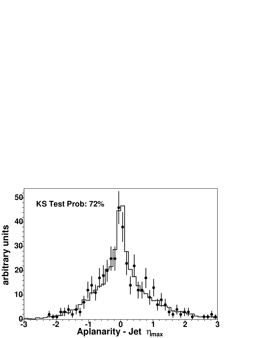
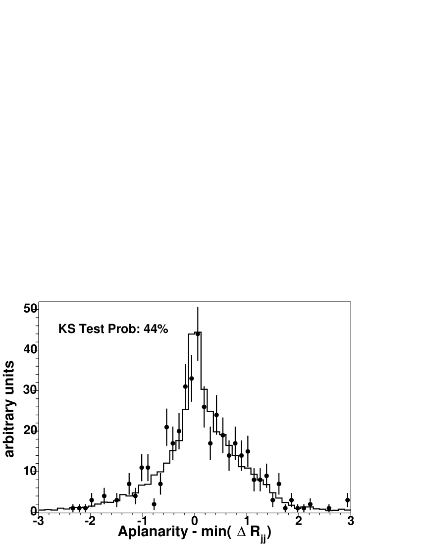
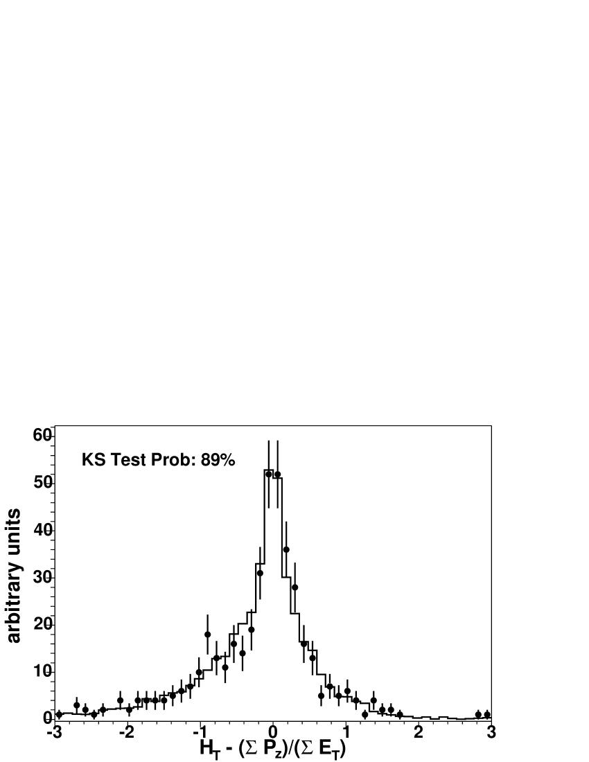
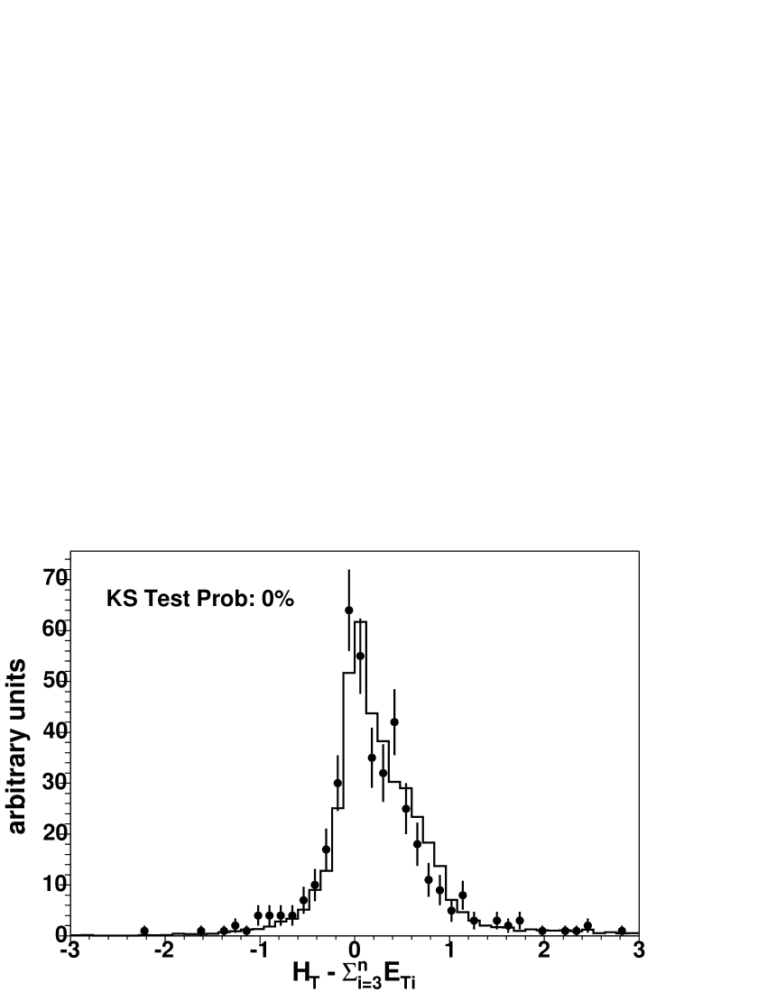
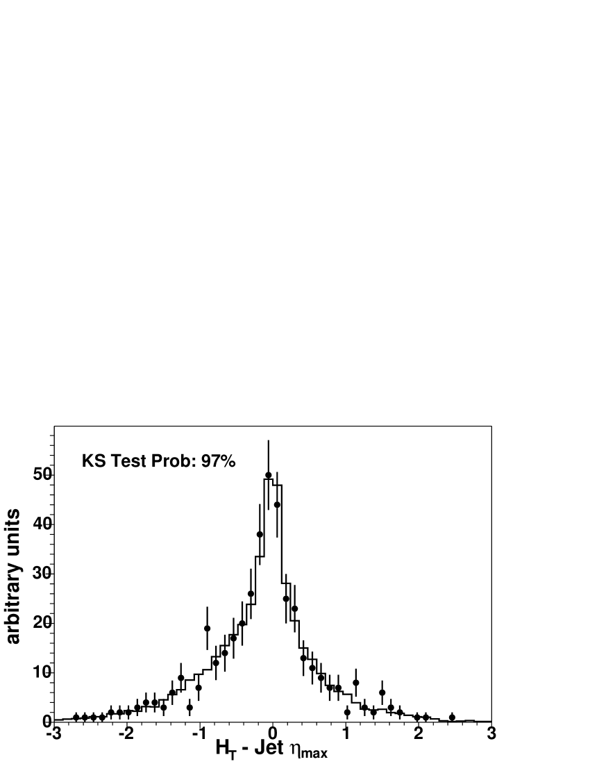
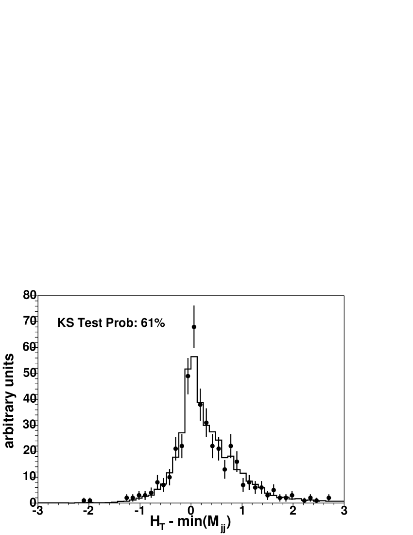
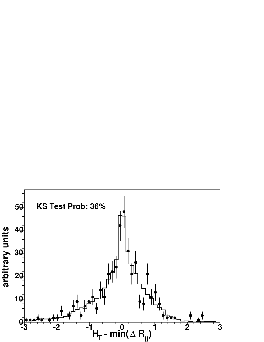
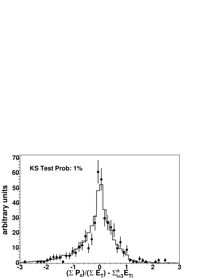
Figure 11: The distributions for the event-by-event correlations between some of the seven ANN input properties for the $W+3$ exclusive jet events compared to the predictions from ALPGEN+HERWIG $W$+3p Monte Carlo and PYTHIA ${t\bar{t}}$ Monte Carlo. The model here is is a combination of 10% ${t\bar{t}}$ and 90% $W$+jets simulated events.

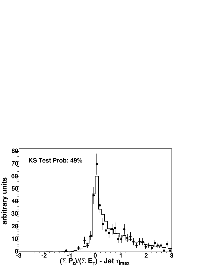
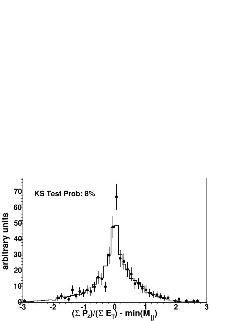
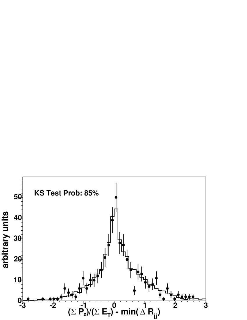
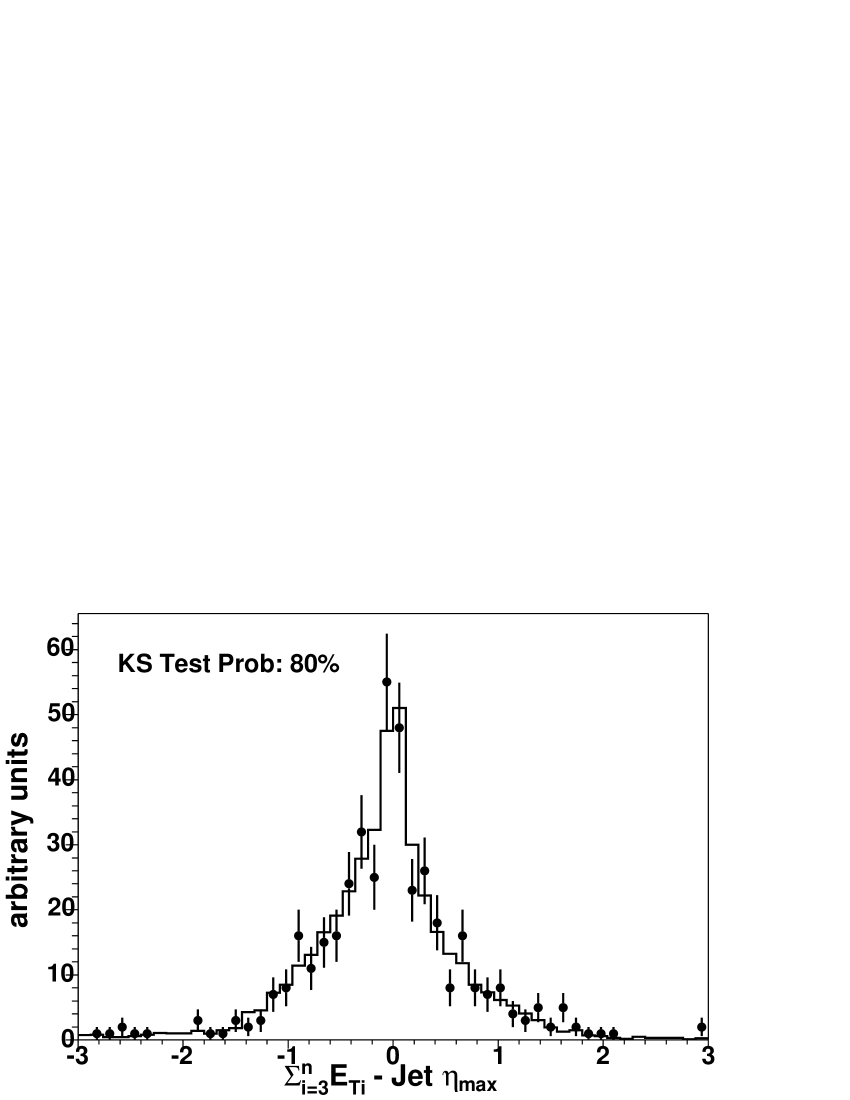
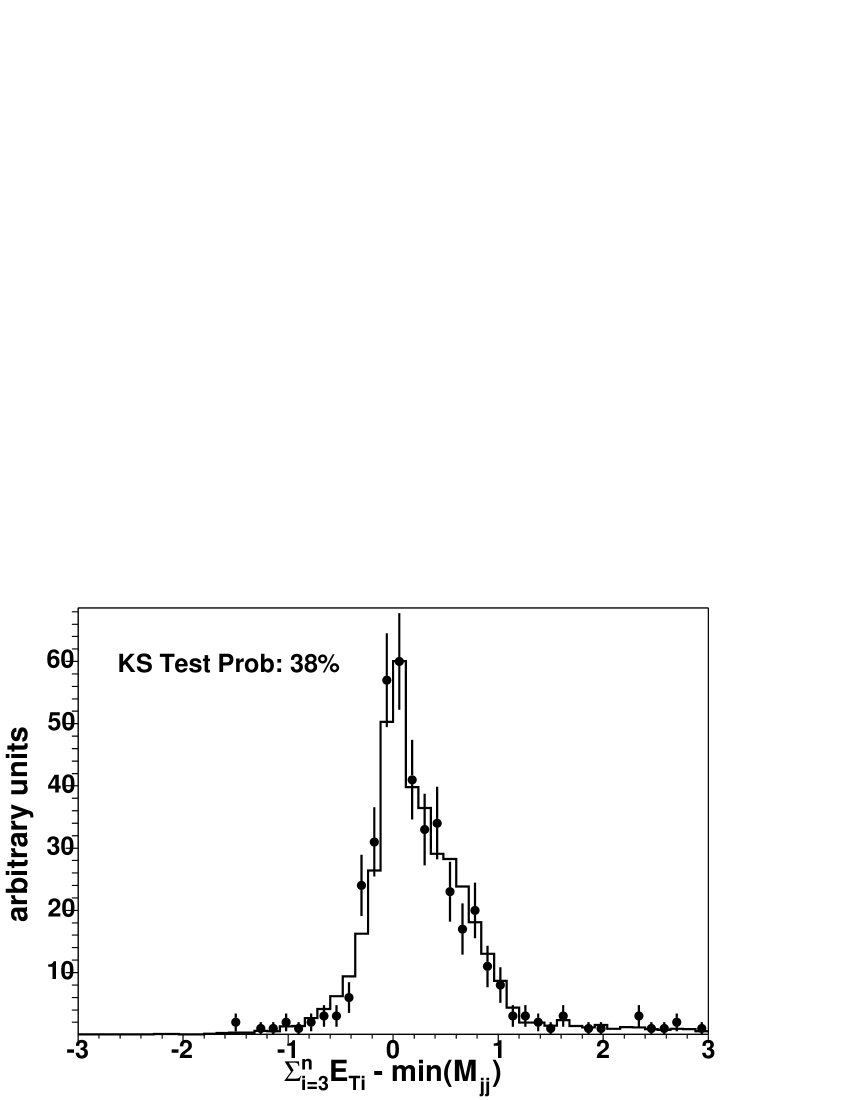
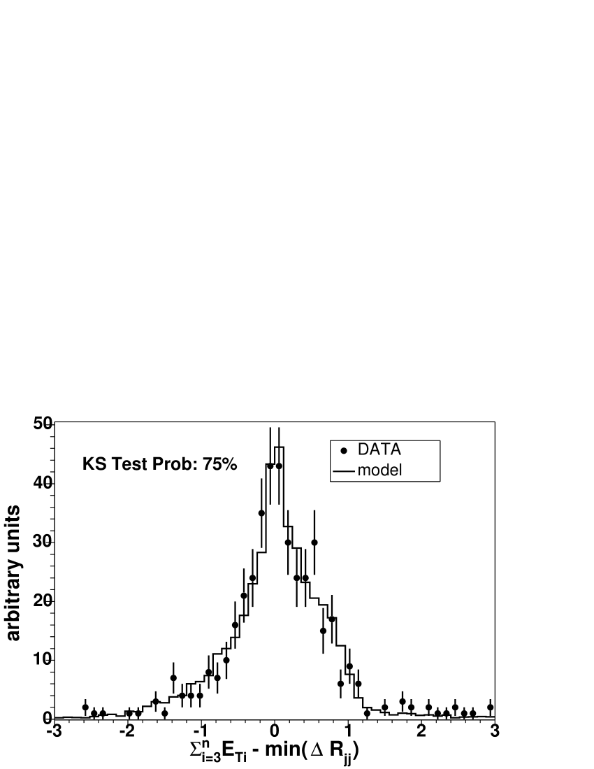
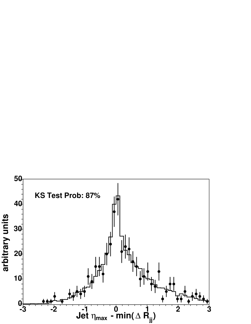
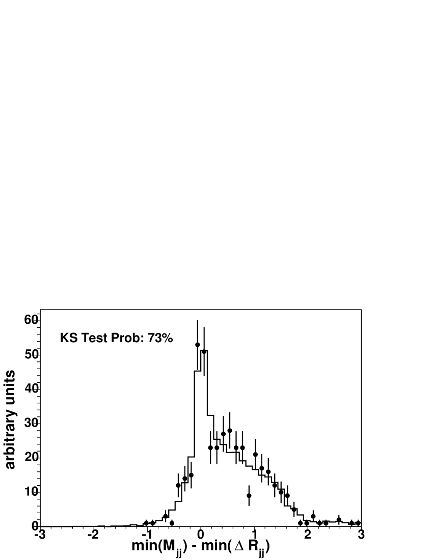
Figure 12: The distributions for the event-by-event correlations between some of the seven ANN input properties for the $W+3$ exclusive jet events compared to the predictions from ALPGEN+HERWIG $W$+3p Monte Carlo and PYTHIA ${t\bar{t}}$ Monte Carlo. The model here is is a combination of 10% ${t\bar{t}}$ and 90% $W$+jets simulated events.

VIII Systematic Uncertainties

Our measurement of the top pair production cross section is sensitive to systematic effects having an impact on the signal acceptance, on the shape of various kinematic distributions, and the luminosity. This last uncertainty is 5.9%, where 4.4% comes from the acceptance and operation of the luminosity monitor and 4.0% from the calculation of the total $p\bar{p}$ cross section cdflumi .

Acceptance systematics fall into sub-categories of those that affect the efficiency of the trigger and lepton identification, and those that affect the efficiency for passing the $\,/\!\!\!\!E_{T}$ and jet ${E_{T}}$ cuts. We quote such systematics in percent (%) as the relative change in the ${t\bar{t}}$ acceptance:

• Lepton Identification Efficiency. For electrons, we consider the uncertainties on the electron energy scale and resolution, the electron momentum scale and resolution, the amount of material in the detector, and the conversion removal efficiency. For muons, we consider the uncertainties on the muon momentum scale and resolution, the modeling of geometrical coverage of the muon detectors, and the cosmic ray removal efficiency. We estimate an uncertainty of 2% from these effects.

• Lepton Isolation. $Z\rightarrow\ell\ell$ candidates provide a clean sample of high $p_{T}$ leptons that can be used to estimate a correction factor for the difference in lepton identification efficiency between data and simulation. However, the leptons from ${t\bar{t}}$ decays tend to be less isolated than the leptons from $Z$ decays. To account for this different environment, we calculate the correction factor as a function of lepton isolation for $Z$ events and then use the lepton isolation distribution in ${t\bar{t}}$ PYTHIA Monte Carlo to obtain an appropriately weighted correction factor. We estimate an uncertainty of 5%, which is dominated at the present time by the small statistics in the $Z$ data sample.

• Jet Energy Scale. We estimate an uncertainty of 4.7%, the average of the changes in acceptance from shifting the jet energy scale by the uncertainty discussed in Section III.6.

• ISR/FSR. Jets due to initial state gluon radiation (ISR) may be produced in addition to the jets from the top decay products. We estimate the uncertainty associated with the modeling of ISR by taking half the change in acceptance for two Monte Carlo samples. These have different $\Lambda_{\textrm{Q}CD}$ values and K-factors for the transverse momentum scale of the ISR evolution. The range of variation was determined by taking the extremes of a range determined by a study of Drell-Yan $Z\rightarrow\ell\ell$ events in data and Monte Carlo. The uncertainty from the modeling of final state gluon radiation (FSR) is estimated by applying these same variations to the FSR evolution. In addition to the hard scattering process and initial and final state radiation, remnants of the proton and anti-proton interaction affect event kinematics. We use a PYTHIA ${t\bar{t}}$ Monte Carlo sample, where the parameters used to describe the charged particle multiplicity in di-jet data have been re-tuned assuming less ISR RickFieldref , to estimate the uncertainty from the modeling of the underlying event. We estimate a total uncertainty of 3% from these effects.

• Parton Distribution Functions. The uncertainty in the distribution of the proton(anti-proton) momentum amongst its constituent partons affects the relative contributions of the $q\bar{q}$ and $gg$ processes to ${t\bar{t}}$ production as well as the momentum of the ${t\bar{t}}$ system. In the CTEQ parametrization the parton distribution functions (PDFs) are described by 20 independent eigenvectors. In a next to the leading order (NLO) version of PDFs, CTEQ6M, a 90% confidence interval is provided for each eigenvector. For the maximum and minimum value of each eigenvector, we compute a new acceptance by re-weighting our default CTEQ5L PYTHIA ${t\bar{t}}$ sample. We add in quadrature the difference between the weighted acceptance for the twenty eigenvectors with respect to the weighted acceptance from the central CTEQ6M and find an uncertainty of 0.5%. The dominant contribution is from the eigenvector most closely associated with the gluon distribution function at large-$x$, which changes the contribution of the $gg$ process from 11% to 21%. We also take the difference of 1.0% between the acceptance for the leading order CTEQ5L, with a 5% contribution from the $gg$ process, and the central value from next to leading order CTEQ6M, with a 15% contribution from the $gg$ process. We find a consistent value for the acceptance from CTEQ5L and the alternative MRST set MRST . The uncertainty from $\alpha_{s}$ is estimated by comparing the weighted acceptance for MRST with $\alpha_{s}=0.1125$ and $\alpha_{s}=0.1175$, which is 1.0%. Adding these three contributions in quadrature, we obtain a total uncertainty of 1.5%.

• Generator. We compare PYTHIA to HERWIG, after correcting for the lack of QED FSR from leptons in HERWIG and for the default HERWIG $W\rightarrow\ell\nu$ branching ratio of 11.1%. We find an acceptance uncertainty due the choice of ${t\bar{t}}$ event generator of 1.4%.

To evaluate the effect of systematic changes in the shapes of kinematic distributions, we use simulated experiments, as described in Section VI.1. In this case, we fit the simulated “data” distribution to signal and background distributions from our default model, and also to signal and background distributions from a model with a particular systematic effect applied. For example, an alternative shape for the ANN output distribution is obtained by processing a set of Monte Carlo simulated events modified according to a particular systematic effect with the network trained using the nominal Monte Carlo samples. The average difference in the fitted number of signal events, relative to the expected number listed in Table 5, is quoted in percent (%) as a systematic uncertainty.

• Jet Energy Scale. A change in the jet energy scale affects the total transverse energy and simultaneously five of the seven kinematic properties used in the ANN. Fig. 13 demonstrates that for an increase in the jet energy scale, the $H_{T}$ distribution for the ${t\bar{t}}$ signal shifts upward significantly, while the the distribution for the $W$+jets background remains almost unchanged. This is due to the large number of $W$+jets background events adjacent to the event selection threshold. For instance, a systematic increase in the jet energy scale means that many $W$+jets background events with a third jet that previously just failed the kinematic requirement will now pass the event selection. These new events tend to have low values of $H_{T}$ and so compensate for the increased $H_{T}$ of the original $W$+jets background events. Fig. 13 also shows that the better separation afforded by the ANN means that the ANN technique is less sensitive to this effect. We estimate an uncertainty of 26% for $H_{T}$ and 17% for the ANN.

  

  

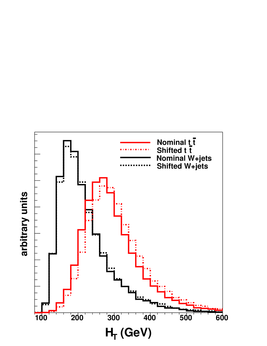
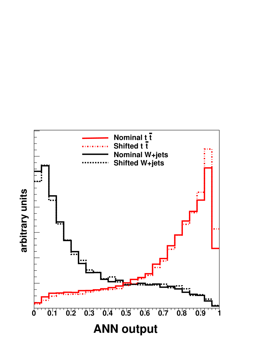
  Figure 13: The $H_{T}$ and ANN distributions for the default jet energy scale and a positive shift corresponding to the uncertainty on the jet energy scale. The distributions are normalized to equal area.

• $\mathbf{W}$+jets background. The uncertainty on the $W$+jets background shape is calculated from ALPGEN+HERWIG samples having different values for the scale of momentum transfer, $Q^{2}$, in the hard scattering process. This affects the initial parton distribution functions and the relative weight of diagrams in the leading order matrix element. We find that the largest change arises between using our default $Q^{2}=M_{W}^{2}+\sum_{i}p_{T,i}^{2}$, which changes on an event-by-event basis, and setting $Q^{2}=4M_{W}^{2}$ which is the same for every event. We estimate an uncertainty of 24.6% for $H_{T}$ and 10.2% for the ANN.

• QCD multi-jet background. We first recall that we expect electrons from unidentified photon conversions to form a large fraction of this background in the electron channel, as we discussed in Section V. Therefore, we use the identified conversions in data to provide a model alternative to our default electron and muon non-isolated data samples. For the uncertainty on the multi-jet background normalization, we vary the contribution by ${}^{+100}_{-50}$% around the central value listed in Table 9. We assign this level of uncertainty from the difference between our estimates listed in Table 9 and the amounts of multi-jet background preferred by a fit to the higher statistics $W$+1 jet and $W$+2 jet regions in Section VII.

• Other electroweak backgrounds. We estimate this systematic as half the difference between including and not including these backgrounds in our model of the $H_{T}$ and ANN output shape.

The systematic uncertainties are summarized in Table 12 for $H_{T}$ and in Table 13 for ANN. When the same systematic effect has an impact on both the ${t\bar{t}}$ acceptance and the shape of the ${t\bar{t}}$ kinematic distributions, we treat the uncertainties as 100% correlated and calculate the total uncertainty by adding the acceptance and shape systematic numbers linearly. For multiple component systematic uncertainties like those from PDFs, ISR and FSR, the acceptance and shape uncertainties for each component are first combined linearly, then the components are added in quadrature. Finally, the overall systematic uncertainty is obtained by adding the total contributions from uncorrelated effects in quadrature.

Table 12: Systematic uncertainties in % on the cross section, for fits to the total transverse energy, $H_{T}$, in the $W+\geq$3 jets sample. The overall uncertainty is given by the sum in quadrature of the numbers in the last column.

Effect	Acceptance (%)	Shape (%)	Total (%)
Jet $E_{T}$ Scale	4.7	21.4	26.1
W+jets Q2 Scale	-	24.6	24.6
QCD fraction	-	2.4	2.4
QCD shape	-	4.5	4.5
Other EWK	-	1.8	1.8
${t\bar{t}}$ PDF	1.5	2.2	4.7
${t\bar{t}}$ ISR	2.1	1.1	2.9
${t\bar{t}}$ FSR	1.7	1.5	3.7
${t\bar{t}}$ generator	1.4	1.0	2.4
Lepton ID/trigger	2.0	-	2.0
Lepton Isolation	5.0	-	5.0
Luminosity	-	-	5.9
Overall			37.8

Table 13: Systematic uncertainties in % on the cross section, for fits to the ANN output distribution in the $W+\geq$3 jets sample. The overall uncertainty is given by the sum in quadrature of the numbers in the last column.

Effect	Acceptance (%)	Shape (%)	Total (%)
Jet $E_{T}$ Scale	4.7	12.2	16.9
W+jets Q2 Scale	-	10.2	10.2
QCD fraction	-	0.6	0.6
QCD shape	-	1.1	1.1
Other EWK	-	2.0	2.0
${t\bar{t}}$ PDF	1.5	2.9	4.4
${t\bar{t}}$ ISR	2.1	1.9	3.0
${t\bar{t}}$ FSR	1.7	1.0	2.7
${t\bar{t}}$ generator	1.4	0.3	1.7
Lepton ID/trigger	2.0	-	2.0
Lepton Isolation	5.0	-	5.0
Luminosity	-	-	5.9
Overall			22.3

IX Results

We have applied the method described in Section VI to a dataset with an integrated luminosity of 194 pb^-1, where 519 events pass the $W+\geq$3 jets selection criteria (Table 5). Figures 14 and 15 show the distribution of data events for the single property, $H_{T}$  and the output of an ANN respectively. We maximize the likelihood of Equation 1 to extract the most probable number of ${t\bar{t}}$ signal events:

$\mu_{{t\bar{t}}}=65.8\pm 21.8$ ($H_{T}$),

$\mu_{{t\bar{t}}}=91.0\pm 15.6$ (ANN),

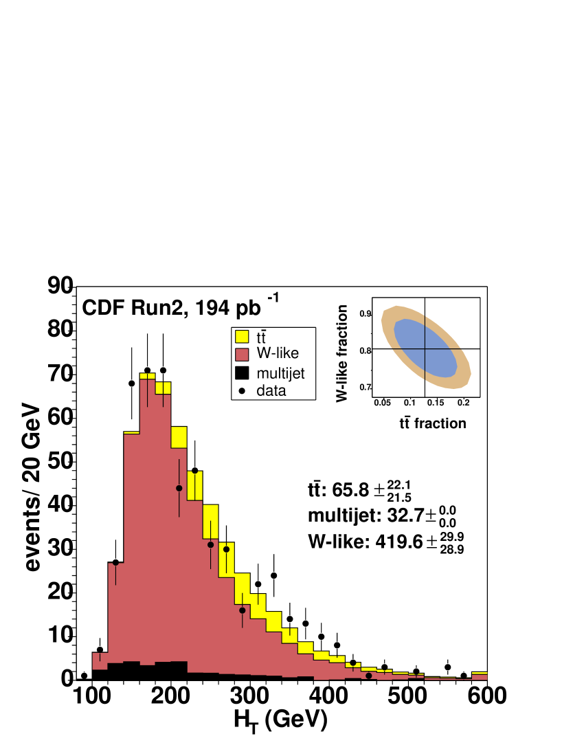
Figure 14: Distribution of observed $H_{T}$ in the $W+\geq$3 jets sample, compared with the result of the fit. The inset shows the 1- and 2-standard-deviation contours of the free parameters in the fit, normalized to the total number of observed events. The contribution of multi-jet background to the fit is fixed.

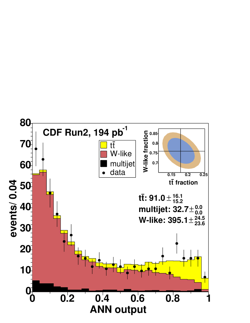
Figure 15: Distribution of observed ANN output in the $W+\geq$3 jets sample, compared with the result of the fit. The inset shows the 1- and 2-standard-deviation contours of the free parameters in the fit, normalized to the total number of observed events. The contribution of multi-jet background to the fit is fixed.

where the uncertainty is statistical only and we have assumed a top mass of 175 GeV/$c^{2}$. Using our estimate of 7.11$\pm$0.56% for the ${t\bar{t}}$ acceptance and 194$\pm$11 pb^-1 for the integrated luminosity in Equation 2, we measure a top pair production cross section of:

$\sigma_{{t\bar{t}}}=4.8\pm 1.6\pm 1.8$ pb ($H_{T}$),

$\sigma_{{t\bar{t}}}=6.6\pm 1.1\pm 1.5$ pb (ANN),

where the uncertainties are statistical and systematic, respectively. These results agree well with the theoretical prediction of $6.7\pm^{0.7}_{0.9}$ pb mlm for a top mass of 175 GeV/$c^{2}$. From simulated experiments with this top mass, we estimate a probability of 10% to find a difference equal to or larger than the observed difference between the results from the correlated $H_{T}$ and ANN distributions. The observed 33% statistical uncertainty for the $H_{T}$ fit is slightly larger than we would expect in 68% of simulated experiments. However, the observed 17% uncertainty for the ANN fit is close to the median from simulated experiments.

We note that both the acceptance and the kinematic distributions for ${t\bar{t}}$ depend on our assumed value for the top quark mass. We quote the dependence of our result for the top pair production cross section on the assumed top quark mass in Table 14. Fig. 16 compares the ANN result with the theoretical predictions mlm ; kidonakis .

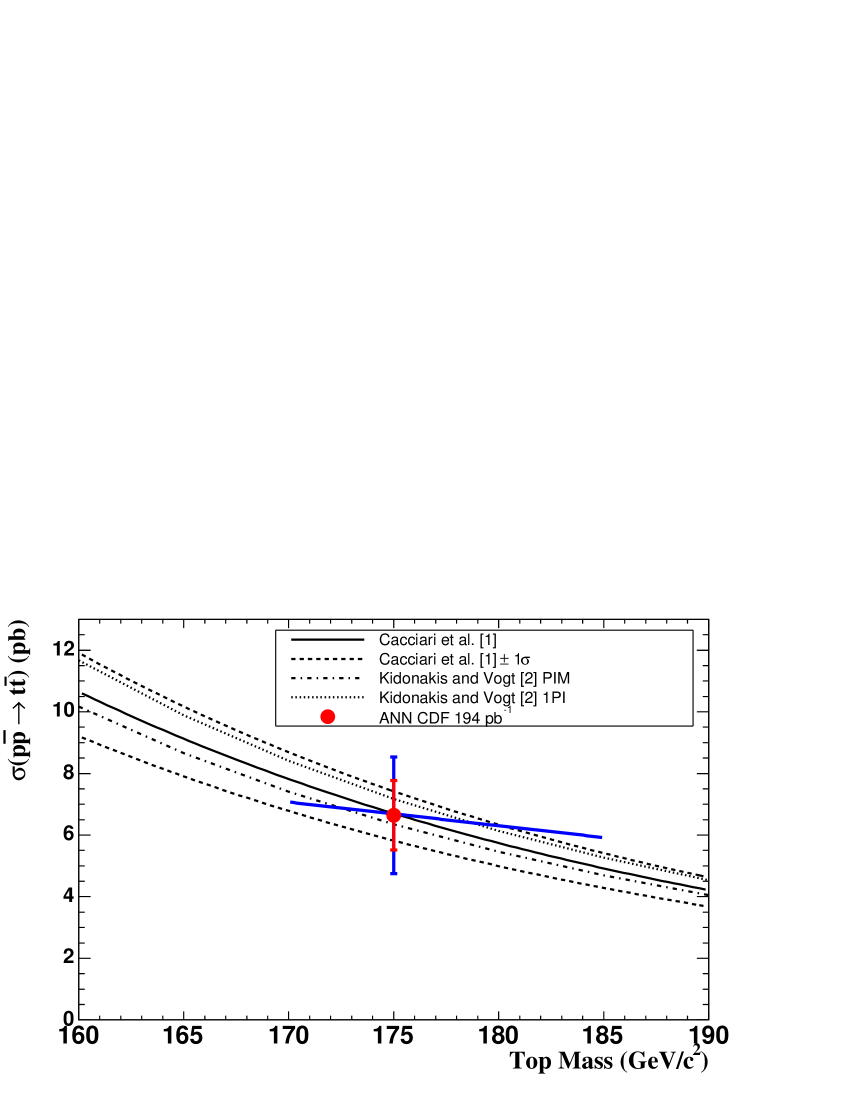
Figure 16: Theoretical predictions for the top quark pair production cross sectionmlm ; kidonakis compared to our measurement with the ANN in the $W+\geq$3 jets data sample. The nearly horizontal error bar shows how the central value of our measurement evolves with top quark mass between 170 and 185 GeV/$c^{2}$.

Table 14: The ${t\bar{t}}$ production cross section results (pb) in the $W+\geq$3 jets sample at different top quark masses. The uncertainty is statistical only.

Generated Top Mass	$\sigma_{{t\bar{t}}}$ from $H_{T}$	$\sigma_{{t\bar{t}}}$ from ANN
160	5.2$\pm$2.1	7.9$\pm$1.3
165	5.1$\pm$1.9	7.5$\pm$1.3
170	4.9$\pm$1.7	7.0$\pm$1.2
175	4.8$\pm$1.6	6.6$\pm$1.1
180	4.5$\pm$1.4	6.3$\pm$1.1
185	4.4$\pm$1.3	5.9$\pm$1.0
190	4.2$\pm$1.2	5.7$\pm$1.0

X Cross-Checks

We found the smallest expected statistical and systematic uncertainties a priori for the ANN in the $W+\geq$3 jets data sample. As a cross-check, we repeat the analysis in the $W+\geq$4 jet sample, where there is a higher expected signal fraction of about 42%. We find 118 events pass the event selection criteria in our data sample with an integrated luminosity of 194 pb^-1. Figures 17 and 18 show the distribution of data events for $H_{T}$ and an ANN specially trained to obtain good separation in the $W+\geq$4 jet sample. We extract the most probable number of ${t\bar{t}}$ signal events:

$\mu_{{t\bar{t}}}=57.1\pm 15.7$ ($H_{T}$),

$\mu_{{t\bar{t}}}=55.3\pm 11.7$ (ANN),

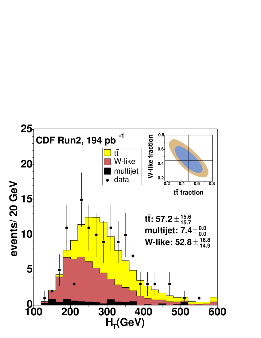
Figure 17: Distribution of observed $H_{T}$ in the $W+\geq$4 jets sample, compared with the result of the fit. The inset shows the 1- and 2-standard-deviation contours of the free parameters in the fit,, normalized to the total number of observed events. The contribution of multi-jet background to the fit is fixed.

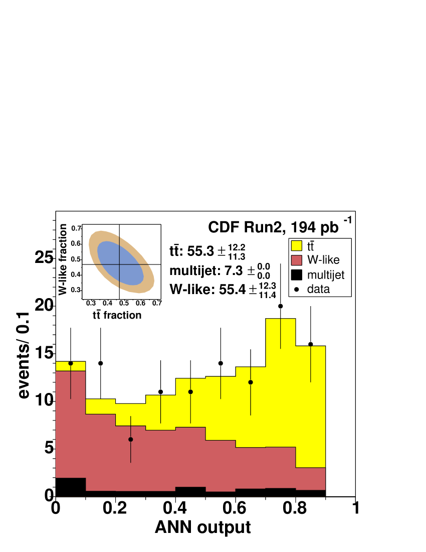
Figure 18: Distribution of observed ANN output in the $W+\geq$4 jets sample, compared with the result of the fit. The inset shows the 1- and 2-standard-deviation contours of the free parameters in the fit, normalized to the total number of observed events. The contribution of multi-jet background to the fit is fixed.

where the uncertainty is statistical only and we have assumed a top mass of 175 GeV/$c^{2}$. The requirement of a fourth jet with transverse energy above 15 GeV reduces the ${t\bar{t}}$ acceptance to 3.85$\pm$0.47%. The measured top pair production cross section is then:

$\sigma_{{t\bar{t}}}=7.7\pm 2.1\pm 3.5$ pb ($H_{T}$),

$\sigma_{{t\bar{t}}}=7.4\pm 1.6\pm 2.0$ pb (ANN),

where the uncertainties are statistical and systematic, respectively. We observe good agreement here between the results of the $H_{T}$ and ANN fits. From simulated experiments, we estimate a probability of 13% to find a difference equal to or larger than the observed difference between the results from the $H_{T}$ distributions in the correlated $W+\geq$3 jets and $W+\geq$4 jets samples. The observed 27% statistical uncertainty for the $H_{T}$ fit is now on the low edge of what we would expect in 68% of simulated experiments. The observed 22% uncertainty for the ANN fit is close to the median from simulated experiments.

We show the results of a fit to each of the twenty kinematic and topological properties listed in Table 11 for the $W+\geq$3 jet data sample in Fig. 19 and the $W+\geq$4 jets data sample in Fig. 20. Some of these properties are highly correlated with each other. We do not observe any significant difference in the results for properties used or not used by the ANN.

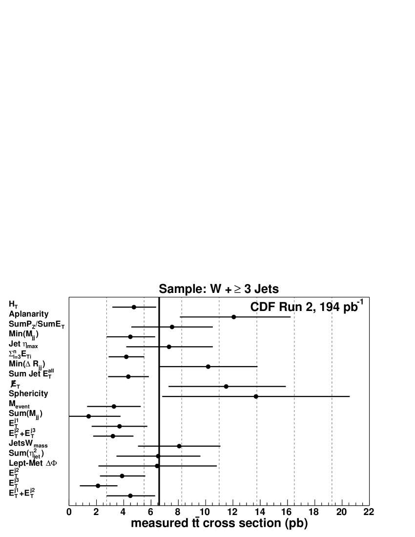
Figure 19: Measured ${t\bar{t}}$ cross section in the $W+\geq$3 jets sample for all twenty kinematic and topological properties considered. The uncertainty is statistical only, the vertical line shows the measured cross section with the ANN of 6.6 pb.

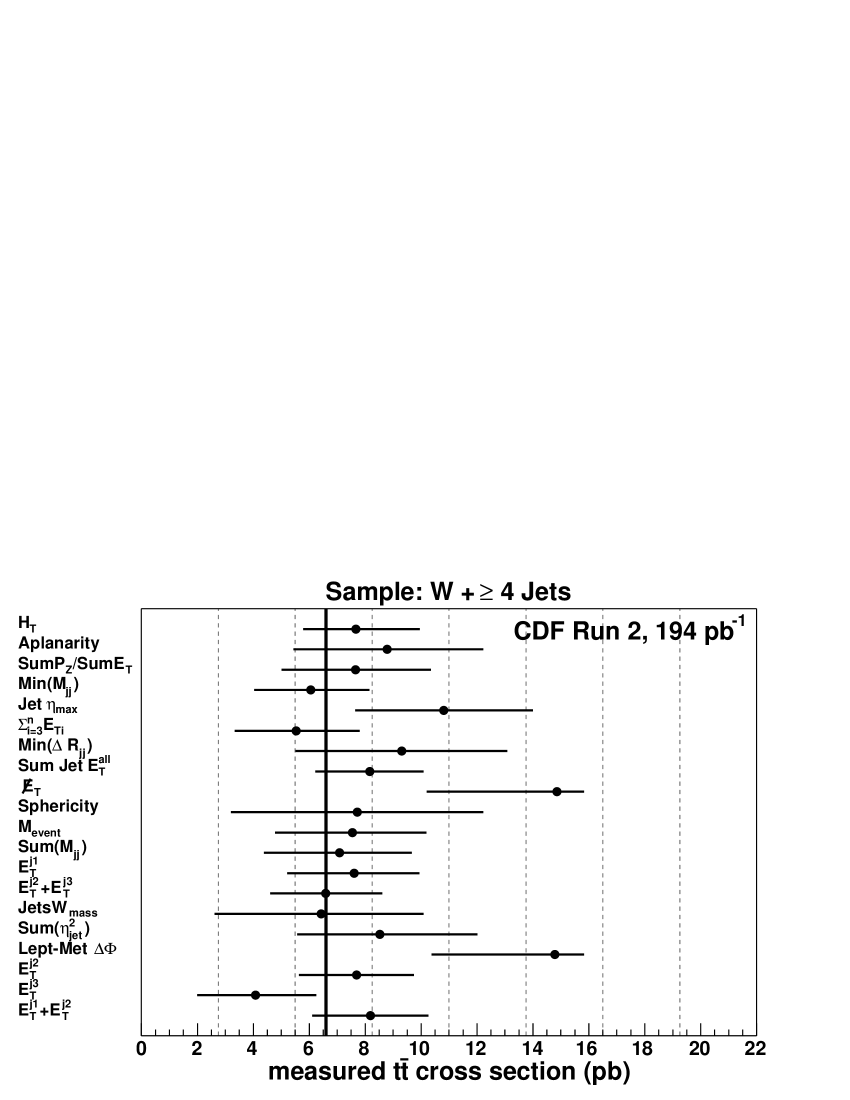
Figure 20: Measured ${t\bar{t}}$ cross section in the $W+\geq$4 jets sample for all twenty kinematic and topological properties. The uncertainty is statistical only, the vertical line shows the measured cross section with the ANN of 6.6 pb.

We note that two other CDF analyses svxruniipaper ; Taka+Mel select a top sample, and measure a top cross section in the lepton+jets channel, by using a displaced secondary vertex to tag the presence of $b$ quarks from the $t\rightarrow Wb$ decay. It is of interest to see how our neural net classifies this top sample. Fig. 21 shows the ANN output for $W+\geq$3 jet data events with, and without, at least one $b$-jet identified using this secondary vertex algorithm. The output of the network is indeed close to 1 for many of the events with at least one identified $b$-jet. This provides verification that the kinematics of the $b$-tagged events are top-like, or, alternatively, the $b$-tag algorithm provides verification that the ANN efficiently isolates top events using kinematics only.

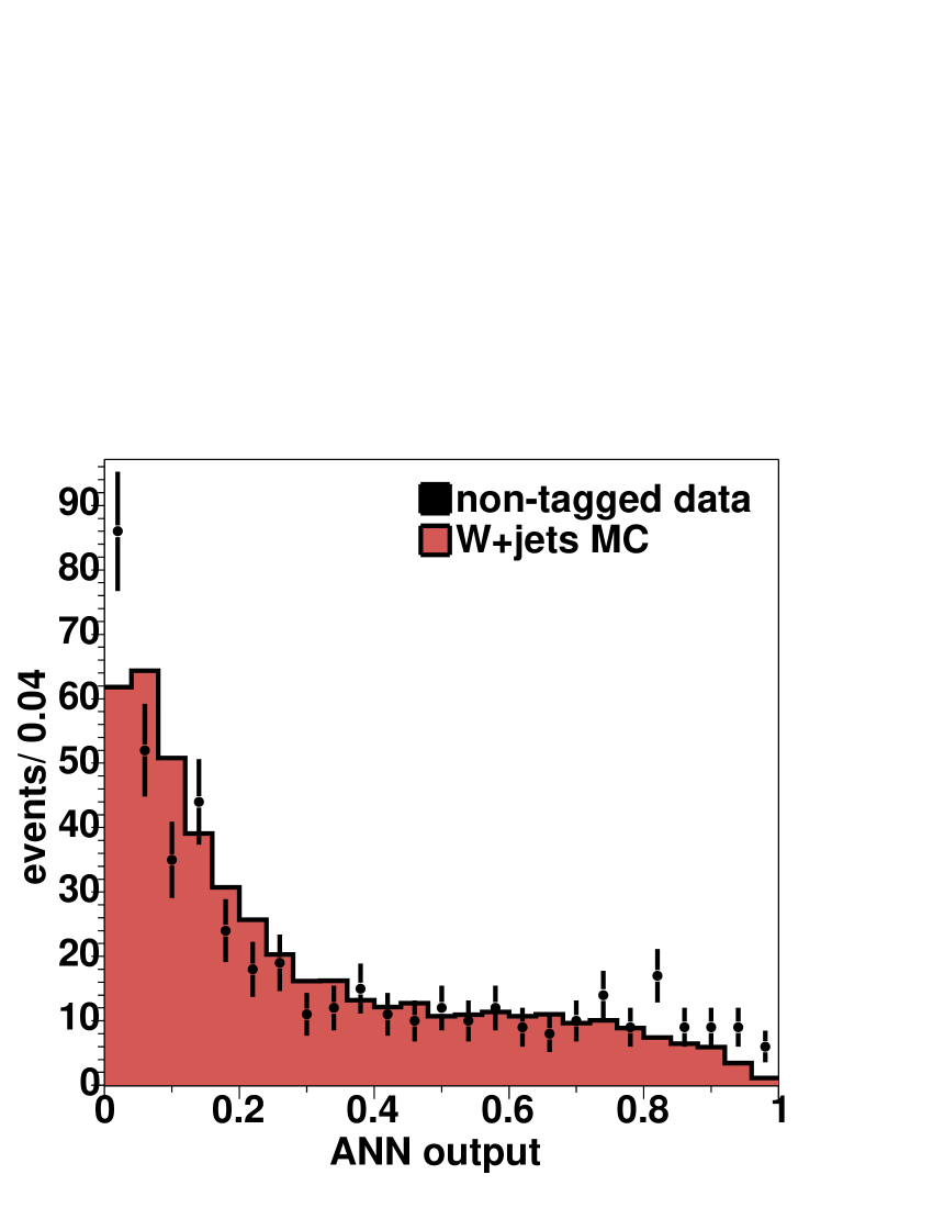
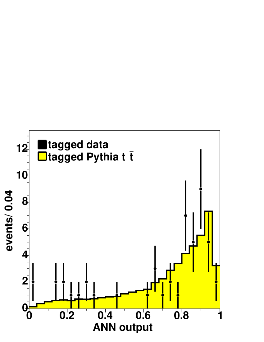
Figure 21: The ANN output for events in the $W+\geq$3 jets data sample with (left) no identified $b$-jet compared to $W$+3 parton ALPGEN+HERWIG Monte Carlo, and (right) at least one identified $b$-jet compared to PYTHIA ${t\bar{t}}$ Monte Carlo. The distributions are normalised to equal area.

XI Conclusions

We present a measurement of the top pair production cross section in $p\overline{p}$ collisions at $\sqrt{s}=1.96$ TeV with an integrated luminosity of 194$\pm$11 pb^-1. We select events in the top lepton+jets channel by requiring one isolated lepton with $E_{T}\geq 20$ GeV, missing transverse energy $\,/\!\!\!\!E_{T}\geq 20$ GeV, and three jets with $E_{T}\geq 15$ GeV. This selection accepts an estimated 7.11 $\pm$ 0.56% of all ${t\bar{t}}$ events. We develop an artificial neural network technique, which combines the information from seven kinematic and topological properties, to discriminate between ${t\bar{t}}$ and background processes. Relative to the discrimination from only the total transverse energy, this artificial neural network technique reduces the expected statistical uncertainty by 30% and the estimated systematic uncertainty by 40%. We perform a binned maximum likelihood fit to the artificial neural network output distribution observed in data, where we rely on Monte Carlo simulation to model the ${t\bar{t}}$ and $W$+jets processes. In a data sample of 519 events, we find 91$\pm$16 ${t\bar{t}}$ events, where the uncertainty is statistical only. We measure a top pair production cross section of $\sigma_{{t\bar{t}}}$=6.6$\pm$1.1 $\pm$1.5 pb, where the uncertainties are statistical and systematic, respectively.

- (1) M. Cacciari, S. Frixione, G. Ridolfi, M. Mangano and P. Nason, JHEP 404:68 (2004).
- (2) N. Kidonakis and R. Vogt, Phys. Rev. D 68, 114014 (2003).
- (3) C.T. Hill and S.J. Parke, Phys. Rev. D 49, 4454 (1994).
- (4) H.P. Nilles, Phys. Rep. 110, 1 (1984); H.E. Haber and G.L. Kane, ibid. 117, 75 (1985).
- (5) H. J. He, N. Polonsky, S. Su, Phys. Rev. D 64 053004 (2001).
- (6) V.A. Novikov, L.B. Okun, A.N. Rozanov, M.I. Vysotsky, Phys. Lett. B 529 111 (2002).
- (7) D. Choudhury, T. M. P. Tait and C. E. M. Wagner, Phys. Rev. D 65, 053002 (2002).
- (8) H. Cheng and I. Low, JHEP 0309:051 (2003).
- (9) D. Chakraborty, J. Konigsberg and D. L. Rainwater, Ann. Rev. Nucl. Part. Sci. 53, 301 (2003).
- (10) CDF Collaboration, F. Abe et al., Phys. Rev. D 51, 4623 (1995).
- (11) CDF Collaboration, F. Abe et al., Phys. Rev. Lett. 75, 3997 (1995).
- (12) CDF Collaboration, D. Acosta et al., Phys. Rev. Lett. 93, 142001 (2004).
- (13) CDF Collaboration, D. Acosta et al., Phys. Rev. D 71, 052003 (2005).
- (14) CDF Collaboration, D. Acosta et al., Phys. Rev. D 72, 032002 (2005).
- (15) CDF Collaboration, F. Abe et al., Phys. Rev. D 59, 092001 (1999).
- (16) CDF Collaboration, D. Acosta et al., Phys. Rev. D 71, 072005 (2005).
- (17) CDF Collaboration, D. Acosta et al., Phys. Rev. D 71, 032001 (2005).
- (18) The detector has cylindrical geometry with forward-backward and axial symmetry around the beam axis. CDF uses a cylindrical coordinate system with the (longitudinal) axis along the proton-beam direction and the azimuthal angle. The pseudo-rapidity of a particle three-momentum is defined in terms of the polar angle of the momentum to the beam direction measured from the point at the center of the detector: .
- (19) T. Affolder et al., Nucl. Instrum. Meth. A 526, 249 (2004).
- (20) C.S. Hill, Nucl. Instrum. Meth. A 530, 1 (2004).
- (21) A. Sill et al., Nucl. Instrum. Meth. A 447, 1 (2000).
- (22) A. Affolder et al., Nucl. Instrum. Meth. A 453, 84 (2000).
- (23) L. Balka et al., Nucl. Instrum. Meth. A 267, 272 (1988).
- (24) S. Bertolucci et al., Nucl. Instrum. Meth. A 267, 301 (1988).
- (25) M. Albrow et al., Nucl. Instrum. Meth. A 453, 245 (2000).
- (26) G. Ascoli et al., Nucl. Instrum. Meth. A 268, 33 (1988).
- (27) D. Acosta et al., Nucl. Instrum. Meth. A 494, 57 (2002).
- (28) When using the total cross section value of mb. S. Klimenko, J. Konigsberg and T. M. Liss, FERMILAB-FN-0741 (2003).
- (29) CDF Collaboration, A. Abulencia et al., arXiv:hep-ex/0508029.
- (30) E.J. Thomson et al. IEEE Trans. Nucl. Sci. 49, 1063 (2002).
- (31) CDF Collaboration, F. Abe et al., Phys. Rev. D 44, 29 (1991).
- (32) CDF Collaboration, T. Affolder et al., Phys. Rev. D 63, 032003 (2001).
- (33) F. Abe et al., Phys. Rev. D 45, 1448 (1992).
- (34) T. Sjostrand et al., Comput. Phys. Commun. 135, 238 (2001).
- (35) G. Corcella et al., JHEP 0101:010 (2001).
- (36) J. Pumplin, D.R. Stump, J. Huston, H.L. Lai, P. Nadolsky, W.K. Tung, JHEP 0207:012 (2002).
- (37) M.L. Mangano, M. Moretti, F. Piccinini, R. Pittau, A.D. Polosa, JHEP 0307:001 (2003).
- (38) S. Catani, F. Krauss, R. Khun and B. R. Webber, JHEP 0111:063 (2001).
- (39) S. Mrenna and P. Richardson, JHEP 0405:040 (2004).
- (40) Brian D. Ripley, Pattern recognition and Neural Networks, Cambridge University Press, Cambridge, England (1996).
- (41) J. Hertz, K. Anders, R. G. Plamer, Introduction to the theory of neural computation, Addison-Wesley, Boston (1991).
- (42) M. Richard and R. Lippmann, Neural Comput. 3, 461 (1991).
- (43) Cartsen Peterson, Thorsteinn Röngnvaldsson, Leif Lönnblad, Comput. Phys. Commun. 81, 185 (1994).
- (44) S. Lawrence, C. L. Giles, A. C. Tsoi, AAAI-97, AAAI Press, Menlo Park California, pp 540-545 (1997).
- (45) M. Dobbs et al., arXiv:hep-ph/0403100, pp 17-24 (2004).
- (46) A. D. Martin, R. G. Roberts, W. J. Stirling, R.S. Thorne, Phys. Lett. B 604, 61 (2004).