First measurement of the $\pi^{+}\pi^{-}$ atom lifetime

Abstract

The goal of the DIRAC experiment at CERN (PS212) is to measure the $\pi^{+}\pi^{-}$ atom lifetime with $10\%$ precision. Such a measurement would yield a precision of $5\%$ on the value of the $S$-wave $\pi\pi$ scattering lengths combination $\left|a_{0}-a_{2}\right|$. Based on part of the collected data we present a first result on the lifetime, $\tau=\left[2.91~{}^{+0.49}_{-0.62}\right]\times 10^{-15}$ s, and discuss the major systematic errors. This lifetime corresponds to $\left|a_{0}-a_{2}\right|=0.264~{}^{+0.033}_{-0.020}~{}m_{\pi}^{-1}$.

, , , , , , , , , , , , , , , , , , , , , , , , , , , , , , , , , , , , , , , , , , , , , , , , , , , , , , , , , , , , , , , , , , , , , , , , , , , , , , , , , , , , , , , ,

1 Introduction

The aim of the DIRAC experiment at CERN [1] is to measure the lifetime of pionium, an atom consisting of a $\pi^{+}$ and a $\pi^{-}$ meson ($A_{2\pi}$). The lifetime is dominated by the charge-exchange scattering process ($\pi^{+}\pi^{-}\rightarrow\pi^{0}\pi^{0}$) and is thus related to the relevant scattering lengths [4]. The partial decay width of the atomic ground state (principal quantum number $n=1$, orbital quantum number $l=0$) is [2, 5, 6, 7, 8, 9]

$$\Gamma_{1S}=\frac{1}{\tau_{1S}}=\frac{2}{9}\;\alpha^{3}\;p\left|a_{0}-a_{2}\right|^{2}(1+\delta)\$$ (1)

with $\tau_{1S}$ the lifetime of the atomic ground state, $\alpha$ the fine-structure constant, $p$ the $\pi^{0}$ momentum in the atomic rest frame, and $a_{0}$ and $a_{2}$ the $S$-wave $\pi\pi$ scattering lengths for isospin 0 and 2, respectively. The term $\delta$ accounts for QED and QCD corrections [6, 7, 8, 9]. It is a known quantity ($\delta=(5.8\pm 1.2)\times 10^{-2}$) ensuring a 1% accuracy for Eq. (1) [8]. A measurement of the lifetime therefore allows to obtain in a model-independent way the value of $|a_{0}-a_{2}|$. The $\pi\pi$ scattering lengths $a_{0}$, $a_{2}$ have been calculated within the framework of Standard Chiral Perturbation Theory [10] with a precision better than 2.5% [11] ($a_{0}=0.220\pm 0.005$, $a_{2}=-0.0444\pm 0.0010$, $a_{0}-a_{2}=0.265\pm 0.004$ in units of inverse pion mass) and lead to the prediction $\tau_{1S}=(2.9\pm 0.1)\times 10^{-15}$ s. The Generalized Chiral Perturbation Theory though allows for larger $a$-values [12]. Model independent measurements of $a_{0}$ have been done using $K_{e4}$ decays [13, 14].

Oppositely charged pions emerging from a high energy proton-nucleus collision may be either produced directly or stem from strong decays (”short-lived” sources) and electromagnetic or weak decays (”long-lived” sources) of intermediate hadrons. Pion pairs from “short-lived” sources undergo Coulomb final state interaction and may form atoms. The region of production being small as compared to the Bohr radius of the atom and neglecting strong final state interaction, the cross section $\sigma^{n}_{A}$ for production of atoms with principal quantum number $n$ is related to the inclusive production cross section for pion pairs from ”short lived” sources without Coulomb correlation ($\sigma^{0}_{s}$) [15] :

$$\frac{d\sigma^{n}_{A}}{d{\vec{p}}_{A}}={(2\pi)}^{3}\frac{E_{A}}{M_{A}}|\Psi_{n}^{C}(\vec{r}^{*}=0)|^{2}\left.\frac{d^{2}\sigma^{0}_{s}}{d{\vec{p}}_{+}d{\vec{p}}_{-}}\right|_{\vec{p}_{+}=\vec{p}_{-}}$$ (2)

with $\vec{p}_{A}$, $E_{A}$ and $M_{A}$ the momentum, energy and mass of the atom in the lab frame, respectively, and $\vec{p}_{+}$, $\vec{p}_{-}$ the momenta of the charged pions. The square of the Coulomb atomic wave function for zero distance $\vec{r}^{*}$ between them in the c.m. system is $|\Psi_{n}^{C}(0)|^{2}=p^{3}_{B}/\pi n^{3}$, where $p_{B}=m_{\pi}\alpha/2$ is the Bohr momentum of the pions and $m_{\pi}$ the pion mass. The production of atoms occurs only in $S$-states [15].

Final state interaction also transforms the “unphysical” cross section $\sigma^{0}_{s}$ into a real one for Coulomb correlated pairs, $\sigma_{C}$ [16, 17]:

$$\frac{d^{2}\sigma_{C}}{d\vec{p}_{+}d\vec{p}_{-}}=|\Psi_{-\vec{k}^{*}}^{C}(\vec{r}^{*})|^{2}\frac{d^{2}\sigma^{0}_{s}}{d\vec{p}_{+}d\vec{p}_{-}},$$ (3)

where $\Psi_{-\vec{k}^{*}}^{C}(\vec{r}^{*})$ is the continuum wave function and $2\vec{k}^{*}\equiv\vec{q}$ with $\vec{q}$ being the relative momentum of the $\pi^{+}$ and $\pi^{-}$ in the c.m. system. $|\Psi_{-\vec{k}^{*}}^{C}(\vec{r}^{*})|^{2}$ describes the Coulomb correlation and at $r^{*}=0$ coincides with the Gamov-Sommerfeld factor $A_{C}(q)$ with $q=|\vec{q}|$ [17]:

$$A_{C}(q)=\frac{2\pi m_{\pi}\alpha/q}{1-\exp(-2\pi m_{\pi}\alpha/q)}\;.$$ (4)

For low $q$, $0\leq q\leq q_{0}$, Eqs. (2, 3, 4) relate the number of produced $A_{2\pi}$ atoms, $N_{A}$, to the number of Coulomb correlated pion pairs, $N_{CC}$ [18] :

$$\frac{N_{A}}{N_{CC}}=\frac{\sigma_{A}^{tot}}{\sigma_{C}^{tot}|_{q\leq q_{0}}}=\frac{(2\pi\alpha m_{\pi})^{3}}{\pi}\frac{\displaystyle{\sum\limits_{n=1}^{\infty}\frac{1}{n^{3}}}}{\displaystyle{\int\limits_{0}^{q_{0}}A_{C}(q)d^{3}q}}=k_{th}(q_{0}).$$ (5)

Eq. (5) defines the theoretical $k$-factor. Throughout the paper we will use

$$q_{0}=2\mathrm{MeV}/c~{}\mathrm{~{}and}~{}k_{th}(q_{0})=0.615.$$ (6)

In order to account for the finite size of the pion production region and of the two-pion final state strong interaction, the squares of the Coulomb wave functions in Eqs. (2) and (3) must be substituted by the square of the complete wave functions, averaged over the distance $\vec{r}^{*}$ and the additional contributions from $\pi^{0}\pi^{0}\rightarrow A_{2\pi}$ as well as $\pi^{0}\pi^{0}\rightarrow\pi^{+}\pi^{-}$ [17]. It should be noticed that these corrections essentially cancel in the $k$-factor (Eq. (5)) and lead to a correction of only a fraction of a percent. Thus finite size corrections can safely be neglected for $k_{th}$.

Once produced, the $A_{2\pi}$ atoms propagate with relativistic velocity (average Lorentz factor $\bar{\gamma}\approx 17$ in our case) and, before they decay, interact with target atoms, whereby they become excited/de-excited or break up. The $\pi^{+}\pi^{-}$ pairs from break-up (atomic pairs) exhibit specific kinematical features which allow to identify them experimentally [15], namely very low relative momentum $q$ and $q_{L}$ (the component of $\vec{q}$ parallel to the total momentum $\vec{p}_{+}+\vec{p}_{-}$) as shown in Fig. 1. After break-up, the atomic pair traverses the target and to some extent loses these features by multiple scattering, essentially in the transverse direction, while $q_{L}$ is almost not affected. This is one reason for considering distributions in $Q_{L}$ as well as in $Q$ when analyzing the data.

Excitation/de-excitation and break-up of the atom are competing with its decay. Solving the transport equations with the cross sections for excitation and break-up, [20, 21, 22, 23, 24, 25, 26, 27, 28, 29, 30, 31] leads to a target-specific relation between break-up probability and lifetime which is estimated to be accurate at the 1% level [22, 32, 33]. Measuring the break-up probability thus allows to determine the lifetime of pionium [15].

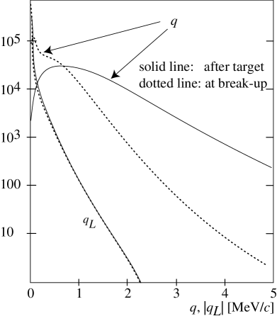
Figure 1: Relative momentum distributions ($q$, $q_{L}$) for atomic $\pi^{+}\pi^{-}$ pairs at the point of break-up and at the exit of the target. Note that $q_{L}$ is almost not affected by multiple scattering in the target.

The first observation of the $A_{2\pi}$ atom [34] has allowed to set a lower limit on its lifetime [18, 19] of $\tau>1.8\times 10^{-15}$ s (90% CL). In this paper we present a determination of the lifetime of the $A_{2\pi}$ atom, based on a large sample of data taken in 2001 with Ni targets.

2 The DIRAC experiment

The DIRAC experiment uses a magnetic double-arm spectrometer at the CERN 24 GeV/$c$ extracted proton beam T8. Details on the set-up may be found in [35]. Since its start-up, DIRAC has accumulated about 15’000 atomic pairs. The data used for this work were taken with two Ni foils, one of 94$\mu$m thickness (76% of the $\pi^{+}\pi^{-}$ data), and one of 98 $\mu$m thickness (24% of the data). An extensive description of the DIRAC set-up, data selection, tracking, Monte Carlo procedures, signal extraction and a first high statistics demonstration of the feasibility of the lifetime measurement, based on the Ni data of 2001, have been published in [36].

The set-up and the definitions of detector acronyms are shown in Fig. 2. The main selection criteria and performance parameters [36] are recalled in the following.

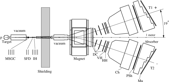
Figure 2: Schematic top view of the DIRAC spectrometer. Upstream of the magnet: target, microstrip gas chambers (MSGC), scintillating fiber detectors (SFD), ionization hodoscopes (IH) and iron shielding. Downstream of the magnet: drift chambers (DC), vertical and horizontal scintillation hodoscopes (VH, HH), gas Cherenkov counters (Ch), preshower detectors (PSh) and, behind the iron absorber, muon detectors (Mu).

Pairs of oppositely charged pions are selected by means of Cherenkov, preshower and muon counters. Through the measurement of the time difference between the vertical hodoscope signals of the two arms, time correlated (prompt) events ($\sigma_{\Delta t}=185$ ps) can be distinguished from accidental events (see [36]). The resolution of the three components of the relative momentum $Q$ of two tracks, transverse and parallel to the c.m. flight direction, $Q_{x}$, $Q_{y}$ and $Q_{L}$, is about $0.5~{}\mathrm{MeV}/c$ for $Q\leq 4$ MeV/$c$. Due to charge combinatorials and inefficiencies of the SFD, the distributions for the transverse components have substantial tails, which the longitudinal component does not exhibit [37]. This is yet another reason for analyzing both $Q$ and $Q_{L}$ distributions.

Data were analyzed with the help of the DIRAC analysis software package ARIANE [39].

The tracking procedures require the two tracks either to have a common vertex in the target plane (“V-tracking”) or to originate from the intersect of the beam with the target (“T-tracking”). In the following we limit ourselves to quoting results obtained with T-tracking. Results obtained with V-tracking do not show significant differences, as will be shown later.

The following cuts and conditions are applied (see [36]):

• at least one track candidate per arm with a confidence level better than 1% and a distance to the beam spot in the target smaller than 1.5 cm in x and y;

• “prompt” events are defined by the time difference of the vertical hodoscopes in the two arms of the spectrometer of $|\Delta t|\leq 0.5$ ns;

• “accidental” events are defined by time intervals $-15\,\mathrm{ns}\leq\Delta t\leq-5$ ns and $7\,\mathrm{ns}\leq\Delta t\leq 17$ ns, determined by the read-out features of the SFD detector (time dependent merging of adjacent hits) and exclusion of correlated $\pi^{-}$p pairs. [36];

• protons in “prompt” events are rejected by time-of-flight in the vertical hodoscopes for momenta of the positive particle below 4 GeV/$c$. Positive particles with higher momenta are rejected;

• $e^{\pm}$ and $\mu^{\pm}$ are rejected by appropriate cuts on the Cherenkov, the preshower and the muon counter information;

• cuts in the transverse and longitudinal components of $Q$ are $Q_{T}\leq 4$ MeV/$c$ and $|Q_{L}|<15$ MeV/$c$. The $Q_{T}$ cut preserves 98% of the atomic signal. The $Q_{L}$ cut preserves data outside the signal region for defining the background;

• only events with at most two preselected hits per SFD plane are accepted. This provides the cleanest possible event pattern.

3 Analysis

The spectrometer including the target is fully simulated by GEANT-DIRAC [38], a GEANT3-based simulation code. The detectors, including read-out, inefficiency, noise and digitalization are simulated and implemented in the DIRAC analysis code ARIANE [39]. The triggers are fully simulated as well.

The simulated data sets for different event types can therefore be reconstructed with exactly the same procedures and cuts as used for experimental data.

The different event types are generated according to the underlying physics.

Atomic pairs: Atoms are generated according to Eq. (2) using measured total momentum distributions for short-lived pairs. The atomic $\pi^{+}\pi^{-}$ pairs are generated according to the probabilities and kinematics described by the evolution of the atom while propagating through the target and by the break-up process (see [40]). These $\pi^{+}\pi^{-}$ pairs, starting from their spatial production point, are then propagated through the remaining part of the target and the full spectrometer using GEANT-DIRAC. Reconstruction of the track pairs using the fully simulated detectors and triggers leads to the atomic pair distribution $dn_{A}^{MC}/dQ$.

Coulomb correlated $\pi^{+}\pi^{-}$ pairs (CC-background): The events are generated according to Eqs. (3,4) using measured total momentum distributions for short-lived pairs. The generated $q$-distributions are assumed to follow phase space modified by the Coulomb correlation function (Eq. (4)), $dN_{CC}^{gen}/dq\propto q^{2}\times A_{C}(q)$. Processing them with GEANT-DIRAC and then analyzing them using the full detector and trigger simulation leads to the Coulomb correlated distribution $dN_{CC}^{MC}/dQ$.

Non-correlated $\pi^{+}\pi^{-}$ pairs (NC-background): $\pi^{+}\pi^{-}$ pairs, where at least one pion originates from the decay of a ”long-lived” source (e.g. electromagnetically or weakly decaying mesons or baryons) do not undergo any final state interactions. Thus they are generated according to $dN_{NC}^{gen}/dq\propto q^{2}$, using slightly softer momentum distributions than for short-lived sources (difference obtained from FRITIOF-6). The Monte Carlo distribution $dN_{NC}^{MC}/dQ$ is obtained as above.

Accidental $\pi^{+}\pi^{-}$ pairs (acc-background): $\pi^{+}\pi^{-}$ pairs, where the two pions originate from two different proton-nucleus interactions, are generated according to $dN_{acc}^{gen}/dq\propto q^{2}$, using measured momentum distributions. The Monte Carlo distribution $dN_{acc}^{MC}/dQ$ is obtained as above.

All the Monte Carlo distributions are normalized, $\int_{0}^{Q_{max}}(dN_{i}^{MC}/dQ)dQ=N_{i}^{MC},~{}i=CC,NC,acc$, with statistics about 5 to 10 times higher than the experimental data; similarly for atomic pairs ($n^{MC}_{A}$).

The measured prompt distributions are approximated by appropriate shape functions. The functions for atomic pairs, $F_{A}(Q)$, and for the backgrounds, $F_{B}(Q)$, (analogously for $Q_{L}$) are defined as:

$$\centering\begin{array}[]{lll}F_{A}(Q)&=&\displaystyle{\frac{n_{A}^{rec}}{n_{A}^{MC}}\frac{dn_{A}^{MC}}{dQ}}\\ F_{B}(Q)&=&\displaystyle{\frac{N_{CC}^{rec}}{N_{CC}^{MC}}\frac{dN_{CC}^{MC}}{dQ}+\frac{N_{NC}^{rec}}{N_{NC}^{MC}}\frac{dN_{NC}^{MC}}{dQ}+\frac{\omega_{acc}N_{pr}}{N_{acc}^{MC}}\frac{dN_{acc}^{MC}}{dQ}}\end{array}\@add@centering$$ (7)

with $n_{A}^{rec},~{}N_{CC}^{rec},~{}N_{NC}^{rec}$ the reconstructed number of atomic pairs, Coulomb- and non-correlated background, respectively, and $\omega_{acc}$ the fraction of accidental background out of all prompt events $N_{pr}$. Analyzing the time distribution measured with the vertical hodoscopes (see [36]) we find $\omega_{acc}$=7.1% (7.7%) for the 94 $\mu$m (98 $\mu$m) data sets [36, 37] and keep it fixed when fitting. The $\chi^{2}$ function for $Q$ (analogously for $Q_{L}$) to minimize is

$$\chi^{2}=\sum_{\nu_{min}}^{\nu_{max}}\frac{\left[\left(\frac{dN_{pr}}{dQ}\Delta Q\right)_{\nu}-\left(\left[F_{A}(Q)+F_{B}(Q)\right]\Delta Q\right)_{\nu}\right]^{2}}{\left(\frac{dN_{pr}}{dQ}\Delta Q\right)_{\nu}+(\sigma_{A})_{\nu}^{2}+(\sigma_{B})_{\nu}^{2}}$$ (8)

with $\Delta Q$ the bin width and $\sigma_{A}$, $\sigma_{B}$ the statistical errors of the Monte Carlo shape functions, which are much smaller than that of the measurement. The fit parameters are $n_{A}^{rec},~{}N_{CC}^{rec},~{}N_{NC}^{rec}$ (see Eq. (7)). As a constraint the total number of measured prompt events is restricted by the condition $N_{pr}~{}(1-\omega_{acc})=N_{CC}^{rec}+N_{NC}^{rec}+n_{A}^{rec}$. The measured distributions as well as the background are shown in Fig. 3 (top).

$\begin{array}[]{cc}\includegraphics[width=203.80193pt]{BS-qtot-fit.eps}&\includegraphics[width=203.80193pt]{BS-ql-fit.eps}\\ \includegraphics[width=203.80193pt]{BS-signalqtot.eps}&\includegraphics[width=203.80193pt]{BS-signalql.eps}\end{array}$

Figure 3: Top: Experimental $Q$ and $Q_{L}$ distributions after subtraction of the prompt accidental background, and fitted Monte Carlo backgrounds (dotted lines). The peak at $Q=4$ MeV/$c$ is due to the cut $Q_{T}\leq 4$ MeV/$c$. Bottom: Residuals after background subtraction. The dotted lines represent the expected atomic signal shape. The bin-width is 0.25 MeV/$c$.

The data taken with 94 and 98 $\mu$m thick targets were analyzed separately. The total number of events in the prompt window is $N_{pr}=471290$.

First, we determine the background composition by minimizing Eq. (8) outside of the atomic pair signal region, i.e. for $Q>4\mathrm{MeV}/c$ and $Q_{L}>2\mathrm{MeV}/c$. For this purpose we require $n_{A}^{rec}=0$. As a constraint, the background parameters $N_{CC}^{rec}$ and $N_{NC}^{rec}$ representing the total number of $CC$- and $NC$-events, have to be the same for $Q$ and $Q_{L}$. Then, with the parameters found, the background is subtracted from the measured prompt distribution, resulting in the residual spectra. For the signal region, defined by the cuts $Q=4\mathrm{MeV}/c$ and $Q_{L}=2\mathrm{MeV}/c$, we obtain the total number of atomic pairs, $n_{A}^{residual}$ and of Coulomb correlated background events, $N_{CC}^{sig}$. Results of fits for $Q$ and $Q_{L}$ together are shown in Table 1.

Table 1: Fit results (94 and 98 $\mu$m targets together, background shapes from Monte Carlo (MC)) for the parameters $N_{CC}^{rec}$ (total number of CC-events), $N_{NC}^{rec}$ (total number of NC events) and $n_{A}^{rec}$ (atomic pairs) and deduced results for the number of atomic pairs from the residuals ($n_{A}^{residual}$) and the number of CC-background events in the signal region ($N_{CC}^{sig}$). MC-a: background fit excluding the signal region. MC-b: fit of the entire momentum range including Monte Carlo shape for atomic pairs (“shape fit”). The cuts were at $Q_{cut}=4\mathrm{MeV}/c$ and $Q_{L,~{}cut}=2\mathrm{MeV}/c$. $Q$ and $Q_{L}$-distributions were fitted together. The normalized $\chi^{2}$ were 0.9 for MC-a and MC-b.

		$N_{CC}^{rec}$	$N_{NC}^{rec}$	$n_{A}^{residual}$	$n_{A}^{rec}$	$N_{CC}^{sig}$
MC-a	Q	$374022\pm 3969$	$56538$	$6518\pm 373$		$106500\pm 1130$
	$Q_{L}$	same	same	$6509\pm 330$		$82289\pm 873$
MC-b	Q	$374282\pm 3561$	$56213$		$6530\pm 294$	$106549\pm 1014$
	$Q_{L}$	same	same		same	$82345\pm 783$

CC-background and NC- or acc-backgrounds are distinguishable due to their different shapes, most pronounced in the $Q_{L}$ distributions (see Fig. 3, top). Accidental and NC-background shapes are almost identical for $Q$ and fully identical for $Q_{L}$ (uniform distributions). Thus, the errors in determining the accidental background $\omega_{acc}$ are absorbed in fitting the NC background. The correlation coefficient between CC and NC background is $-99\%$. This strong correlation leads to equal errors for $N_{CC}^{rec}$ and $N_{NC}^{rec}$. The CC-background is determined with a precision better than 1%. Note that the difference between all prompt events and the background is $N_{pr}-N_{CC}^{rec}-N_{NC}^{rec}-\omega_{acc}N_{pr}=6590$, hence very close to the number of residual atomic pairs ($n_{A}^{residual}$) as expected. This relation is also used as a strict constraint for fits outside of the signal region ($>$), $N_{pr}^{>}-N_{CC}^{rec>}-N_{NC}^{rec>}-(\omega_{acc}N_{pr})^{>}=0$ and, hence, the fit requires only one free parameter, $N_{CC}^{rec>}$.

Second, the atomic pair signal may be directly obtained by minimizing Eq. (8) over the full range and including the Monte Carlo shape distribution $F_{A}$ (“shape fit”). The signal strength has to be the same for $Q$ and $Q_{L}$. The result for the signal strength $n_{A}^{rec}$ as well as the CC-background below the cuts, $N_{CC}^{sig}$, are shown in Table 1. The errors are determined by MINOS [41].

The consistency between the analysis in $Q$ with the one in $Q_{L}$ establishes the correctness of the $Q_{T}$ reconstruction. A 2D fit in the variables ($Q_{L},~{}Q_{T}$) confirms the results of Table 1.

4 Break-up probability

In order to deduce the break-up probability, $P_{br}=n_{A}/N_{A}$, the total number of atomic pairs $n_{A}$ and the total number of produced $A_{2\pi}$ atoms, $N_{A}$, have to be known. None of the two numbers is directly measured. The procedure of obtaining the two quantities requires reconstruction efficiencies and is as follows.

Number of atomic pairs: Using the generator for atomic pairs a large number of events, $n_{A}^{gen}$, is generated in a predefined large spatial acceptance window $\Omega_{gen}$, propagated through GEANT-DIRAC including the target and reconstructed along the standard procedures. The total number of reconstructed Monte Carlo atomic pairs below an arbitrary cut in $Q$, $n_{A}^{MC-rec}(Q\leq Q_{cut})$ defines the reconstruction efficiency for atomic pairs $\epsilon_{A}^{cut}=n_{A}^{MC-rec}(Q\leq Q_{cut})/n_{A}^{gen}$. The total number of atomic pairs is obtained from the measured pairs by $n_{A}=n_{A}^{rec}(Q\leq Q_{cut})/\epsilon_{A}^{cut}$.

Number of produced $A_{2\pi}$ atoms: Here we use the known relation between produced atoms and Coulomb correlated $\pi^{+}\pi^{-}$ pairs (CC-background) of Eq. (5). Using the generator for CC pairs, $N_{CC}^{gen}$ events, of which $N_{CC}^{gen}(q\leq q_{0})$ (see Eq. 6) have $q$ below $q_{0}$, are generated into the same acceptance window $\Omega_{gen}$ as for atomic pairs and processed analogously to the paragraph above to provide the number of reconstructed CC-events below the same arbitrary cut in $Q$ as for atomic pairs, $N_{CC}^{MC-rec}(Q\leq Q_{cut})$. These CC-events are related to the originally generated CC-events below $q_{0}$ through $\epsilon_{CC}^{cut}=N_{CC}^{MC-rec}(Q\leq Q_{cut})/N_{CC}^{gen}(q\leq q_{0})$. The number of produced atoms thus is $N_{A}=k_{th}(q_{0})N_{CC}^{rec}(Q\leq Q_{cut})/\epsilon_{CC}^{cut}$ (see Eq. (6)).

The break-up probability $P_{br}$ thus becomes:

$$P_{br}=\frac{n_{A}}{N_{A}}=\frac{n_{A}^{rec}(Q\leq Q_{cut})}{k(Q_{cut})N_{CC}^{rec}(Q\leq Q_{cut})}\qquad\mathrm{with}\;\;k(Q_{cut})=k_{th}(q_{0})\frac{\epsilon_{A}^{cut}}{\epsilon_{CC}^{cut}}.$$ (9)

In Table 2 the $k$-factors are listed for different cuts in $Q$ and $Q_{L}$ for the two target thicknesses (94$\mu$m and 98$\mu$m) and the weighted average of the two, corresponding to their relative abundances in the Ni data of 2001. The accuracy is of the order of one part per thousand and is due to Monte Carlo statistics.

Table 2: $k(Q_{cut})$ factors as a function of cuts in $Q$ and $Q_{L}$ for the 94 and 98 $\mu$m thick Ni targets, and the weighted average of the two for a relative abundance of 76% (94$\mu$m) and 24% (98$\mu$m).

	$k_{94~{}\mu\mathrm{m}}$	$k_{98~{}\mu\mathrm{m}}$	$k_{average}$
$Q_{cut}=2\mathrm{MeV}/c$	$0.5535\pm 0.0007$	$0.5478\pm 0.0007$	$0.5521\pm 0.0007$
$Q_{cut}=3\mathrm{MeV}/c$	$0.2565\pm 0.0003$	$0.2556\pm 0.0003$	$0.2563\pm 0.0003$
$Q_{cut}=4\mathrm{MeV}/c$	$0.1384\pm 0.0002$	$0.1383\pm 0.0002$	$0.1384\pm 0.0002$
$Q_{L,cut}=1\mathrm{MeV}/c$	$0.3054\pm 0.0004$	$0.3044\pm 0.0003$	$0.3050\pm 0.0004$
$Q_{L,cut}=2\mathrm{MeV}/c$	$0.1774\pm 0.0002$	$0.1776\pm 0.0002$	$0.1774\pm 0.0002$

With the $k$-factors of Table 2 and the measurements listed in Table 1, the break-up probabilities of Table 3 are obtained. The simultaneous fit of $Q$ and $Q_{L}$ with the atomic shape results in a single value.

The break-up probabilities from $Q$ and $Q_{L}$ agree within a fraction of a percent. The values from shape fit and from background fit are in perfect agreement (see Table 1). We adopt the atomic shape fit value of $P_{br}=0.447\pm 0.023_{stat}$, because the fit covers the full $Q$, $Q_{L}$ range and includes correlations between $n_{A}^{rec}$ and $N_{CC}^{sig}$.

Analyzing the data with three allowed hit candidates in the SFD search window instead of two, results in more atomic pairs (see Ref. [36], T-tracking). The break-up probabilities obtained are $0.440\pm 0.024$ and $0.430\pm 0.021$ for $Q$ and $Q_{L}$, respectively. They are not in disagreement with the adopted value of 0.447. Despite the larger statistics, the accuracy is not improved, due to additional background. This background originates from additional real hits in the upstream detectors or from electronic noise and cross-talk. This has been simulated and leads essentially to a reduced reconstruction efficiency but not to a deterioration of the reconstruction quality. The additional sources of systematic uncertainties lead us not to consider this strategy of analysis further on.

V-tracking provides a slightly different data sample, different $k$-factors and different signal strengths and CC-background. The break-up probability, however, does not change significantly and is $P_{br}^{V-tracking}=0.453\pm 0.025_{stat}$, only 0.3 $\sigma$ off from the adopted value 0.447.

The break-up probability has to be corrected for the impurities of the targets. Thus, the 94 $\mu$m thick target has a purity of only 98.4%, while the 98 $\mu$m thick target is 99.98 % pure. The impurities (C, Mg, Si, S, Fe, Cu) being mostly of smaller atomic number than Ni lead (for the weighted average of both targets) to a reduction of the break-up probability of 1.1% as compared to pure Ni, assuming a lifetime of 3$fs$. Therefore, the measured break-up probability has to be increased by 0.005 in order to correspond to pure Ni. The final result is:

$$P_{br}=0.452\pm 0.023_{stat}.$$ (10)

Table 3: Break-up probabilities for the combined Ni2001 data, based on the results of Table 1 and the $k$-factors of Table 2 for the cuts $Q_{cut}=4\mathrm{MeV}/c$ and $Q_{L,cut}=2\mathrm{MeV}/c$ . Errors are statistical.

	$n_{A}^{residual}$	$n_{A}^{rec}$	$N_{CC}^{sig}$	$P_{br}$
$Q$	$6518\pm 373$		$106500\pm 1130$	$0.442\pm 0.026$
$Q_{L}$	$6509\pm 330$		$82289\pm 873$	$0.445\pm 0.023$
$Q$ &$Q_{L}$		$6530\pm 294$	$106549\pm 1004$	$0.447\pm 0.023$

5 Systematic errors

Systematic errors may occur through the analysis procedures and through physical processes which are not perfectly under control. We investigate first procedure-induced errors.

The break-up probability will change, if the ratio $N_{CC}^{rec}/N_{NC}^{rec}$ depends on the fit range. If so, the Monte Carlo distributions do not properly reproduce the measured distributions and the amount of CC-background may not be constant. In Fig. 5 the dependence is shown for the fits in $Q$, $Q_{L}$ and both together. The ratio is reasonably constant within errors, with the smallest errors for a fit range of $Q=Q_{L}=15\mathrm{MeV}/c$. At this point the difference between $Q$ and $Q_{L}$ fits leads to a difference in break-up probability of $\Delta P_{br}^{CC}=0.023$.

Consistency of the procedure requires that the break-up probability does not depend on $Q_{cut}$. In Figure 5 the dependence on the cut is shown for break-up probabilities deduced from $n_{A}^{residual}$. There is a systematic effect which, however, levels off for large cut momenta. This dependence indicates that the shape of the atomic pair signal as obtained from Monte Carlo (and used for the $k$-factor determination) is not in perfect agreement with the residual shape. This may be due to systematics in the atomic pair shape directly and/or in reconstructed CC-background for small relative momenta. The more the signal is contained in the cut, the more the $P_{br}$ values stabilize. As a consequence, we chose a cut that contains the full signal (see Eq. (10)). This argument is also true for sharper cuts in $Q_{T}$ than the one from the event selection. Cut momenta beyond the maximum cut of Figure 5 would only test background, as the signal would not change anymore.

To investigate whether the atomic pair signal shape is the cause of the above cut dependence, we studied two extreme models for atom break-up: break-up only from the 1$S$-state and break-up only from highly excited states. The two extremes result in a difference in break-up probability of $\Delta P_{br}^{shape}=0.008$.

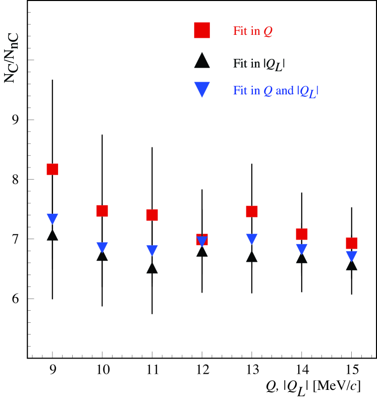
Figure 4: Ratio of CC-background over NC-background as a function of fit range.

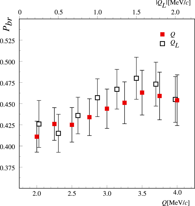
Figure 5: $P_{br}$ as a function of cut momentum for $Q$ and $Q_{L}$.

Sources of systematic errors may also arise from uncertainties in the genuine physical process. We have investigated possible uncertainties in multiple scattering as simulated by GEANT by changing the scattering angle in the GEANT simulation by $\pm 5\%$. As a result, the break-up probability changes by 0.002 per one percent change of multiple scattering angle. In fact we have measured the multiple scattering for all scatterers (upstream detectors, vacuum windows, target) and found narrower angular distributions than expected from the standard GEANT model [42]. This, however, may be due also to errors in determining the thickness and material composition of the upstream detectors. Based on these studies we conservatively attribute a maximum error of +5% and -10% to multiple scattering.

Another source of uncertainty may be due to the presence of unrecognized $K^{+}K^{-}$ and $\bar{p}p$ pairs that would fulfill all selection criteria [43]. Such pairs may be as abundant as 0.5% and 0.15%, respectively, of $\pi^{+}\pi^{-}$ pairs as estimated for $K^{+}K^{-}$ with FRITIOF-6 and for $\bar{p}p$ from time-of-flight measurements in a narrow momentum interval with DIRAC data. Their mass renders the Coulomb correlation much more peaked at low $Q$ than for pions, which leads to a change in effective $\pi^{+}\pi^{-}$ Coulomb background at small $Q$, thus to a smaller atomic pair signal and therefore to a decrease of break-up probability. The effect leads to a change of $\Delta P_{br}^{\bar{K}K,~{}\bar{p}p}=-0.04$. We do not apply this shift but consider it as a maximum systematic error of $P_{br}$. Admixtures from unrecognized $e^{+}e^{-}$ pairs from photon conversion do not contribute because of their different shapes.

Finally, the correlation function Eq. (3) used in the analysis is valid for pointlike production of pions, correlated only by the Coulomb final state interaction (Eq. (4)). However, there are corrections due to finite size and strong interaction [17]. These have been studied based on the UrQMD transport code simulations [44] and DIRAC data on $\pi^{-}\pi^{-}$ correlations. The parameters of the underlying model are statistically fixed with data up to 200 MeV/$c$ relative momentum. For $Q\leq 30$ MeV/$c$, the DIRAC data are too scarce to serve as a test of the model. The corrections lead to a change of $\Delta P_{br}^{finite-size}=-0.02$. Due to the uncertainties we conservatively consider 1.5 times this change as a maximum error, but do not modify $P_{br}$.

The systematics are summarized in Table 4. The extreme values represent the ranges of the assumed uniform probability density function (u.p.d.f.), which, in case of asymmetric errors, were complemented symmetrically for deducing the corresponding standard deviations $\sigma$. Convoluting the five u.p.d.f. results in bell-shaped curves very close to a Gaussian, and the $\pm\sigma$ (Table 4, total error) correspond roughly to a 68.5% confidence level and can be added in quadrature to the statistical error.

The final value of the break-up probability is

$$P_{br}=0.452\pm 0.023_{stat}~{}^{+0.009}_{-0.032}\}_{syst}=0.452~{}^{+0.025}_{-0.039}.$$ (11)

Table 4: Summary of systematic effects on the measurement of the break-up probability $P_{br}$. Extreme values have been transformed into $\sigma$ assuming uniform distributions.

source	extreme values	$\sigma$
CC-background	+0.012 / -0.012	$\pm$0.007
signal shape	+0.004 / -0.004	$\pm$0.002
multiple scattering	+0.01 /-0.02	$~{}^{+0.006}_{-0.013}$
$K^{+}K^{-}$ and $\bar{p}p$	$+0~{}/-0.04$	$~{}^{+0}_{-0.023}$
finite size	$+0~{}/-0.03$	$~{}^{+0}_{-0.017}$
Total	.	$~{}^{+0.009}_{-0.032}$

6 Lifetime of Pionium

The lifetime may be deduced on the basis of the relation between break-up probability and lifetime for a pure Ni target (Fig. 6). This relation, estimated to be accurate at the 1% level, may itself have uncertainties due to the experimental conditions. Thus the target thickness is estimated to be correct to better than $\pm~{}1~{}\mu$m, which leads to an error in the lifetime (for $P_{br}=0.45$) smaller than $\pm~{}0.01$ fs, less than 1% of the expected lifetime and thus negligible. The result for the lifetime is

$$\tau_{1S}=\left[2.91~{}^{+0.45}_{-0.38}\}_{stat}~{}^{+0.19}_{-0.49}\}_{syst}\right]\times 10^{-15}~{}\mathrm{s}=\left[2.91~{}^{+0.49}_{-0.62}\right]\times 10^{-15}~{}\mathrm{s}.$$ (12)

The errors are not symmetric because the $P_{br}-\tau$ relation is not linear, and because finite size corrections and heavy particle admixtures lead to possible smaller values of $P_{br}$. The accuracy achieved for the lifetime is about $+17\%$, almost entirely due to statistics and $-21\%$, due to statistics and systematics in roughly equal parts. With full statistics (2.3 times more than analysed here) the statistical errors may be reduced accordingly. The two main systematic errors (particle admixtures and finite size correction) will be studied in more detail in the future program of DIRAC.

Using Eq. (1), the above lifetime corresponds to $\left|a_{0}-a_{2}\right|=0.264~{}^{+0.033}_{-0.020}~{}m_{\pi}^{-1}$.

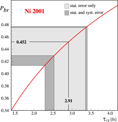
Figure 6: Break-up probability $P_{br}$ as a function of the lifetime of the atomic ground state $\tau_{1S}$ for the combined 94 and 98 $\mu$m thick Ni targets. The experimentally determined $P_{br}$ with statistical and total errors translates into a value of the lifetime with corresponding errors.

7 Acknowledgements

We are indebted to the CERN PS crew for providing a beam of excellent quality. This work was supported by CERN, the Grant Agency of the Czech Republic, grant No. 202/01/0779 and 202/04/0793, the Greek General Secretariat of Research and Technology (Greece), the University of Ioannina Research Committee (Greece), the IN2P3 (France), the Istituto Nazionale di Fisica Nucleare (Italy), the Grant-in-Aid for Scientific Research from Japan Society for the Promotion of Science 07454056, 08044098, 09640376, 09440012, 11440082, 11640293, 11694099, 12440069, 14340079, and 15340205, the Ministry of Education and Research, under project CORINT No.1/2004 (Romania), the Ministery of Industry, Science and Technologies of the Russian Federation and the Russian Foundation for Basic Research (Russia), under project 01-02-17756, the Swiss National Science Foundation, the Ministerio de Ciencia y Tecnologia (Spain), under projects AEN96-1671 and AEN99-0488, the PGIDT of Xunta de Galicia (Spain).

References

- [1] B. Adeva et al., DIRAC proposal, CERN/SPSLC 95-1, SPSLC/P 284 (1995).
- [2] J. Uretsky and J. Palfrey, Phys. Rev. 121 (1961) 1798.
- [3] H.-W. Hammer and J.N. Ng, Eur. Phys.J. A6 (1999) 115.
- [4] S. Deser et al., Phys. Rev. 96 (1954) 774.
- [5] S.M. Bilenky et al., Yad. Phys. 10 (1969) 812; (Sov. J. Nucl. Phys. 10 (1969) 469).
- [6] H. Jallouli and H. Sazdjian, Phys. Rev. D58 (1998) 014011; Erratum: ibid., D58 (1998) 099901.
- [7] M.A. Ivanov et al. Phys. Rev. D58 (1998) 094024.
- [8] J. Gasser et al., Phys. Rev. D64 (2001) 016008; hep-ph/0103157.
- [9] A. Gashi et al., Nucl. Phys. A699 (2002) 732.
- [10] S. Weinberg, Physica A96 (1979) 327; J. Gasser and H. Leutwyler, Phys. Lett. B125 (1983) 325; ibid Nucl. Phys. B250 465, 517, 539.
- [11] G. Colangelo, J. Gasser and H. Leutwyler, Nucl. Phys. B603 (2001) 125.
- [12] M. Knecht et al., Nucl. Phys. B457 (1995) 513.
- [13] L. Rosselet et al., Phys. Rev. D15 (1977) 547.
- [14] S. Pislak et al., Phys. Rev. Lett, 87 (2001) 221801.
- [15] L.L. Nemenov, Yad. Fiz. 41 (1985) 980; (Sov. J. Nucl. Phys. 41 (1985) 629).
- [16] A.D.Sakharov, Z.Eksp.Teor.Fiz. 18 (1948) 631.
- [17] R. Lednicky, DIRAC note 2004-06, nucl-th/0501065.
- [18] L.G. Afanasyev, O.O. Voskresenskaya, V.V.Yazkov, Communication JINR P1-97-306, Dubna, 1997.
- [19] L.G. Afanasyev et al., Phys. Lett. B338 (1994) 478.
- [20] L.S. Dulian and A.M. Kotsinian, Yad.Fiz. 37 (1983) 137; (Sov. J. Nucl. Phys. 37 (1983) 78).
- [21] S. Mrówczyński, Phys. Rev. A33 (1986) 1549; S.Mrówczyński, Phys. Rev. D36 (1987) 1520; K.G. Denisenko and S. Mrówczyński, ibid. D36 (1987) 1529.
- [22] L.G. Afanasyev and A.V. Tarasov, Yad.Fiz. 59 (1996) 2212; (Phys. At. Nucl. 59 (1996) 2130).
- [23] Z. Halabuka et al., Nucl.Phys. B554 (1999) 86–102.
- [24] A.V. Tarasov and I.U. Khristova, JINR-P2-91-10, Dubna 1991.
- [25] O.O. Voskresenskaya, S.R. Gevorkyan and A.V. Tarasov, Phys. At. Nucl. 61 (1998) 1517.
- [26] L. Afanasyev, A. Tarasov and O. Voskresenskaya, J.Phys. G 25 (1999) B7.
- [27] D.Yu. Ivanov, L. Szymanowski, Eur.Phys.J. A5 (1999) 117.
- [28] T.A. Heim et al., J. Phys. B33 (2000) 3583.
- [29] T.A. Heim et al., J. Phys. B34 (2001) 3763.
- [30] M. Schumann et al., J. Phys. B35 (2002) 2683.
- [31] L. Afanasyev, A. Tarasov and O. Voskresenskaya, Phys.Rev.D 65 (2002) 096001; hep-ph/0109208.
- [32] C. Santamarina, M. Schumann, L.G. Afanasyev and T. Heim, J.Phys. B 36 (2003) 4273.
- [33] L. Afanasyev et al., J. Phys B37 (2004) 4749.
- [34] L.G. Afanasyev et al., Phys. Lett. B308 (1993) 200.
- [35] B. Adeva B et al., Nucl.Instr.Meth. A515 (2003) 467.
- [36] B. Adeva et al. J. Phys. G30 (2004) 1929.
- [37] Ch. P. Schuetz, “Measurement of the breakup probability of atoms in a Nickel target with the DIRAC spectrometer”, PhD Thesis, Basel, March 2004, http://cdsweb.cern.ch/searc.py?recid=732756.
- [38] P. Zrelov and V. Yazkov, “The GEANT-DIRAC Simulation Program”, DIRAC note 1998-08, http://zrelov.home.cern.ch/zrelov/dirac/montecarlo/instruction/instruct26.html
- [39] D. Drijard, M. Hansroul and V. Yazkov, The DIRAC offline user’s Guide, and /afs/cern.ch/user/d/diracoff/public/offline/docs
- [40] C. Santamarina and Ch. P. Schuetz, DIRAC note 2003-9.
- [41] F. James and M. Roos, Function Minimization and Error Analysis, Minuit, CERN Program Library, D506 MINUIT
- [42] A. Dudarev et al., DIRAC note 2005-02.
- [43] O.E. Gortchakov and V.V. Yazkov, DIRAC note 2005-01.
- [44] S. A. Bass et al., Prog. Part. Nucl.Phys. 41 (1998) 225.