Measurement of Time-Dependent $C\!P$-Violating Asymmetries and Constraints on $\sin(2\beta+\gamma)$ with Partial Reconstruction of $B\rightarrow D^{*\mp}\pi^{\pm}$ Decays

Abstract

We present a measurement of the time-dependent $C\!P$-violating asymmetries in decays of neutral $B$ mesons to the final states $D^{*\mp}\pi^{\pm}$, using approximately $232$ million $B\kern 1.79993pt\overline{\kern-1.79993ptB}{}$ events recorded by the BABAR experiment at the PEP-II $e^{+}e^{-}$ storage ring. Events containing these decays are selected with a partial reconstruction technique, in which only the high-momentum $\pi^{\pm}$ from the $B$ decay and the low-momentum $\pi^{\mp}$ from the $D^{*\mp}$ decay are used. We measure the parameters related to $2\beta+\gamma$ to be $a_{D^{*}\pi}=-0.034\pm 0.014\pm 0.009$ and $c_{D^{*}\pi}^{\ell}=-0.019\pm 0.022\pm 0.013$. With some theoretical assumptions, we interpret our results in terms of the lower limits $|\sin(2\beta+\gamma)|>0.62~{}(0.35)$ at 68% (90%) confidence level.

I INTRODUCTION

The Cabibbo-Kobayashi-Maskawa (CKM) quark-mixing matrix ref:km provides an explanation of $C\!P$ violation and is under experimental investigation aimed at constraining its parameters. A crucial part of this program is the measurement of the angle $\gamma=\arg{\left(-V_{ud}V_{ub}^{\ast}/V_{cd}V_{cb}^{\ast}\right)}$ of the unitarity triangle related to the CKM matrix. The decay modes $B\rightarrow{D^{*}}^{\mp}\pi^{\pm}$ have been proposed for use in measurements of $\sin(2\beta+\gamma)$ ref:book , where $\beta=\arg{\left(-V_{cd}V_{cb}^{\ast}/V_{td}V_{tb}^{\ast}\right)}$ is well measured ref:sin2b . In the Standard Model the decays $B^{0}\rightarrow D^{*}{{}^{-}}\pi^{+}$ and $\kern 1.79993pt\overline{\kern-1.79993ptB}{}^{0}\rightarrow D^{*}{{}^{-}}\pi^{+}$ proceed through the $\overline{b}\rightarrow\overline{c}u\overline{d}$ and $b\rightarrow u\bar{c}d$ amplitudes $A_{c}$ and $A_{u}$. Fig. 1 shows the tree diagrams contributing to these decays. The relative weak phase between $A_{u}$ and $A_{c}$ in the usual Wolfenstein convention ref:wolfen is $\gamma$. When combined with $B^{0}\kern 1.79993pt\overline{\kern-1.79993ptB}{}^{0}$ mixing, this yields a weak phase difference of $2\beta+\gamma$ between the interfering amplitudes.

Figure 1: Feynman diagrams for the Cabibbo-favored decay $B^{0}\rightarrow D^{*}{{}^{-}}\pi^{+}$ (left), corresponding to the decay amplitude $A_{c}$, and the Cabibbo-suppressed decay $\kern 1.79993pt\overline{\kern-1.79993ptB}{}^{0}\rightarrow D^{*}{{}^{-}}\pi^{+}$ (right), whose amplitude is $A_{u}$.

In $\mathchar 28935\relax(4{\rm S})\rightarrow B\kern 1.79993pt\overline{\kern-1.79993ptB}{}$ decays, the decay rate distribution for $B\rightarrow{D^{*}}^{\mp}\pi^{\pm}$ is

$${\cal P}^{\pm}_{\eta}(\Delta t) = {e^{-|\Delta t|/\tau}\over 4\tau}\times\left[1\mp S^{\zeta}\sin(\Delta m\Delta t)\right.$$ (1)

$$\left.\mp\eta C\cos(\Delta m\Delta t)\right],$$

where $\tau$ is the $B^{0}$ lifetime averaged over the two mass eigenstates, $\Delta m$ is the $B^{0}\kern 1.79993pt\overline{\kern-1.79993ptB}{}^{0}$ mixing frequency, and $\Delta t$ is the difference between the time of the $B\rightarrow{D^{*}}^{\mp}\pi^{\pm}$ ($B_{\rm rec}$) decay and the decay of the other $B$ ($B_{\rm tag}$) in the event. The upper (lower) signs in Eq. (1) indicate the flavor of the $B_{\rm tag}$ as a $B^{0}$ ($\kern 1.79993pt\overline{\kern-1.79993ptB}{}^{0}$), while $\eta=+1$ ($-1$) and $\zeta=+$ ($-$) for the $B_{\rm rec}$ final state ${D^{*}}^{-}\pi^{+}$ (${D^{*}}^{+}\pi^{-}$). The parameters $C$ and $S^{\pm}$ are given by

$$C\equiv{1-r^{*2}\over 1+r^{*2}}\,,\ \ \ \ S^{\pm}\equiv{2{r^{*}}\over 1+r^{*2}}\,\sin(2\beta+\gamma\pm\delta^{*}).$$ (2)

Here $\delta^{*}$ is the strong phase difference between $A_{u}$ and $A_{c}$, and ${r^{*}}=|A_{u}/A_{c}|$. Since $A_{u}$ is doubly CKM-suppressed with respect to $A_{c}$, one expects ${r^{*}}\approx\left|\frac{V_{ub}V_{cd}^{\ast}}{V_{cb}^{\ast}V_{ud}}\right|=0.02$.

We report a study of the $C\!P$-violating asymmetry in $B\rightarrow D^{*\mp}\pi^{\pm}$ decays using the technique of partial reconstruction, which allows us to achieve a high efficiency for the selection of signal events. We use approximately twice the integrated luminosity of our previous analysis of this process ref:run1-2 , and employ an improved method to eliminate a measurement bias, as described in Sec. III.6.2. Many of the tools and procedures used in this analysis were validated in a previous analysis dedicated to the measurement of the $B^{0}$ lifetime ref:dstpi-lifetime .

In this analysis, terms of order $r^{*2}$, to which we currently have no sensitivity, have been neglected. The interpretation of the measured asymmetries in terms of $\sin(2\beta+\gamma)$ requires an assumption regarding the value of ${r^{*}}$, discussed in Sec. VI.

II THE BABAR DETECTOR AND DATASET

The data used in this analysis were recorded with the BABAR detector at the PEP-II asymmetric-energy storage rings, and consist of 211 fb^-1 collected on the $\mathchar 28935\relax(4{\rm S})$ resonance (on-resonance sample), and 21 fb^-1 collected at an $e^{+}e^{-}$ center-of-mass (CM) energy approximately 40 $\mathrm{\,Me\kern-1.00006ptV}$ below the resonance peak (off-resonance sample). Samples of Monte Carlo (MC) ref:geant4 events with an equivalent luminosity approximately four times larger than the data sample were analyzed using the same reconstruction and analysis procedure.

The BABAR detector is described in detail in Ref. ref:babar . We provide a brief description of the main components and their use in this analysis. Charged-particle trajectories are measured by a combination of a five-layer silicon vertex tracker (SVT) and a 40-layer drift chamber (DCH) in a 1.5-T solenoidal magnetic field. Tracks with low transverse momentum can be reconstructed in the SVT alone, thus extending the charged-particle detection down to transverse momenta of about 50 ${\mathrm{\,Me\kern-1.00006ptV\!/}c}$. We use a ring-imaging Cherenkov detector (DIRC) for charged-particle identification and augment it with energy-loss measurements from the SVT and DCH. Photons and electrons are detected in a CsI(Tl) electromagnetic calorimeter (EMC), with photon-energy resolution $\sigma_{E}/E=0.023(E/\mathrm{\,Ge\kern-1.00006ptV})^{-1/4}\oplus 0.014$. The instrumented flux return (IFR) is equipped with resistive plate chambers to identify muons.

III ANALYSIS METHOD

III.1 Partial Reconstruction of $B\rightarrow D^{*\mp}\pi^{\pm}$

In the partial reconstruction of a $B\rightarrow D^{*\mp}\pi^{\pm}$ candidate ($B_{\rm rec}$), only the hard (high-momentum) pion track $\pi_{h}$ from the $B$ decay and the soft (low-momentum) pion track $\pi_{s}$ from the decay $D^{*-}\rightarrow\kern 1.99997pt\overline{\kern-1.99997ptD}{}^{0}\pi_{s}^{-}$ are used. The cosine of the angle between the momenta of the $B$ and the hard pion in the CM frame is then computed:

$$\cos\theta_{Bh}={M_{{D^{*}}^{-}}^{2}-M_{B^{0}}^{2}-M_{\pi}^{2}+E_{\rm CM}E_{h}\over 2p_{B}|\vec{p}_{h}|},$$ (3)

where $M_{x}$ is the nominal mass of particle $x$ ref:pdg2004 , $E_{h}$ and $\vec{p}_{h}$ are the measured CM energy and momentum of the hard pion, $E_{\rm CM}$ is the total CM energy of the incoming $e^{+}e^{-}$ beams, and $p_{B}=\sqrt{E_{\rm CM}^{2}/4-M_{B^{0}}^{2}}$. Events are required to be in the physical region $|\cos\theta_{Bh}|<1$. Given $\cos\theta_{Bh}$ and the measured momenta of the $\pi_{h}$ and $\pi_{s}$, the $B$ four-momentum can be calculated up to an unknown azimuthal angle $\phi$ around ${\vec{p}}_{h}$. For every value of $\phi$, the expected $D$ four-momentum $p_{D}(\phi)$ is determined from four-momentum conservation, and the corresponding $\phi$-dependent invariant mass $m(\phi)\equiv\sqrt{|p_{D}(\phi)|^{2}}$ is calculated. We define the missing mass $m_{\rm miss}\equiv{1\over 2}\left[m_{\rm max}+m_{\rm min}\right]$, where $m_{\rm max}$ and $m_{\rm min}$ are the maximum and minimum values of $m(\phi)$. In signal events, $m_{\rm miss}$ peaks at the nominal $D^{0}$ mass $M_{D^{0}}$, with a gaussian width of about 3 ${\mathrm{\,Me\kern-1.00006ptV\!/}c^{2}}$ (Fig. 2). The $m_{\rm miss}$ distribution for combinatoric background events is significantly broader, making the missing mass the primary variable for distinguishing signal from background. The discrimination between signal and background provided by the $m_{\rm miss}$ distribution is independent of the choice of the value of $\phi$. With the arbitrary choice $\phi=0$, we use four-momentum conservation to calculate the CM $D$ and $B$ momentum vectors, which are used as described below.

III.2 Backgrounds

In addition to $B\rightarrow D^{*\mp}\pi^{\pm}$ events, the selected event sample contains the following kinds of events:

• $B\rightarrow D^{*\mp}\rho^{\pm}$.

• Peaking $B\kern 1.79993pt\overline{\kern-1.79993ptB}{}$ background, defined as decays other than $B\rightarrow D^{*\mp}\rho^{\pm}$, in which the $\pi_{h}$ and $\pi_{s}$ originate from the same $B$ meson, with the $\pi_{s}$ originating from a charged $D^{*}$ decay. The $m_{\rm miss}$ distribution of these events peaks broadly under the signal peak.

• Combinatoric $B\kern 1.79993pt\overline{\kern-1.79993ptB}{}$ background, defined as all remaining $B\kern 1.79993pt\overline{\kern-1.79993ptB}{}$ background events.

• Continuum $e^{+}e^{-}\rightarrow q\overline{q}$, where $q$ represents a $u$, $d$, $s$, or $c$ quark.

III.3 Event Selection

To suppress the continuum background, we select events in which the ratio of the 2nd to the 0th Fox-Wolfram moment ref:R2 , computed using all charged particles and EMC clusters not matched to tracks, is smaller than 0.40. Hard-pion candidates are required to be reconstructed with at least twelve DCH hits. Kaons and leptons are rejected from the $\pi_{h}$ candidate lists based on information from the IFR and DIRC, energy loss in the SVT and DCH, or the ratio of the candidate’s EMC energy deposition to its momentum ($E/p)$.

We define the $D^{*}$ helicity angle $\theta_{D^{*}}$ to be the angle between the flight directions of the $D$ and the $B$ in the $D^{*}$ rest frame. Taking advantage of the longitudinal polarization in signal events, we suppress background by requiring $|\cos\theta_{D^{*}}|$ to be larger than 0.4.

All candidates are required to satisfy $m_{\rm miss}>1.81$ ${\mathrm{\,Ge\kern-1.00006ptV\!/}c^{2}}$. Multiple candidates are found in 5% of the events. In these instances, only the candidate with the $m_{\rm miss}$ value closest to $M_{D^{0}}$ is used.

III.4 Fisher Discriminant

To further discriminate against continuum events, we combine fifteen event-shape variables into a Fisher discriminant ref:fisher $F$. Discrimination originates from the fact that $q\overline{q}$ events tend to be jet-like, whereas $B\kern 1.79993pt\overline{\kern-1.79993ptB}{}$ events have a more spherical energy distribution. Rather than applying requirements to the variable $F$, we maximize the sensitivity by using it in the fits described below. The fifteen variables are calculated using two sets of particles. Set 1 includes all tracks and EMC clusters, excluding the hard and soft pion candidates; Set 2 is composed of Set 1, excluding all tracks and clusters with CM momentum within 1.25 radian of the CM momentum of the $D$. The variables, all calculated in the CM frame, are 1) the scalar sum of the momenta of all Set 1 tracks and EMC clusters in nine $20^{\circ}$ angular bins centered about the hard pion direction; 2) the value of the sphericity, computed with Set 1; 3) the angle with respect to the hard pion of the sphericity axis, computed with Set 2; 4) the direction of the particle of highest energy in Set 2 with respect to the hard pion; 5) the absolute value of the vector sum of the momenta of all the particles in Set 2; 6) the momentum $|\vec{p}_{h}|$ of the hard pion and its polar angle.

III.5 Decay Time Measurement and Flavor Tagging

To perform this analysis, $\Delta t$ and the flavor of the $B_{\rm tag}$ must be determined. We tag the flavor of the $B_{\rm tag}$ using lepton or kaon candidates. The lepton CM momentum is required to be greater than 1.1 ${\mathrm{\,Ge\kern-1.00006ptV\!/}c}$ to suppress leptons that originate from charm decays. If several flavor-tagging tracks are present in either the lepton or kaon tagging category, the only track of that category used for tagging is the one with the largest value of $\theta_{T}$, the CM angle between the track momentum and the momentum of the “missing” (unreconstructed) $D$. The tagging track must satisfy $\cos\theta_{T}<C_{T}$, where $C_{T}=0.75$ ($C_{T}=0.50$) for leptons (kaons), to minimize the impact of tracks originating from the decay of the missing $D$. If both a lepton and a kaon satisfy this requirement, the event is tagged with the lepton.

We measure $\Delta t$ using $\Delta t=(z_{\rm rec}-z_{\rm tag})/(\gamma\beta c)$, where $z_{\rm rec}$ ($z_{\rm tag}$) is the decay position of the $B_{\rm rec}$ ($B_{\rm tag}$) along the beam axis ($z$) in the laboratory frame, and the $e^{+}e^{-}$ boost parameter $\gamma\beta$ is calculated from the measured beam energies. To find $z_{\rm rec}$, we use the $\pi_{h}$ track parameters and errors, and the measured beam-spot position and size in the plane perpendicular to the beams (the $x-y$ plane). We find the position of the point in space for which the sum of the $\chi^{2}$ contributions from the $\pi_{h}$ track and the beam spot is a minimum. The $z$ coordinate of this point determines $z_{\rm rec}$. The beam spot has an r.m.s. size of approximately 120 $\mu$m in the horizontal dimension ($x$), 5 $\mu$m in the vertical dimension ($y$), and 8.5 mm along the beams ($z$). The average $B$ flight in the $x-y$ plane is 30 $\mu$m. To account for the $B$ flight in the beam-spot-constrained vertex fit, 30 $\mu$m are added to the effective $x$ and $y$ sizes for the purpose of conducting this fit.

In lepton-tagged events, the same procedure, with the $\pi_{h}$ track replaced by the tagging lepton, is used to determine $z_{\rm tag}$.

In kaon-tagged events, we obtain $z_{\rm tag}$ from a beam-spot-constrained vertex fit of all tracks in the event, excluding $\pi_{h}$, $\pi_{s}$ and all tracks within 1 radian of the $D$ momentum in the CM frame. If the contribution of any track to the $\chi^{2}$ of the vertex is more than 6, the track is removed and the fit is repeated until no track fails the $\chi^{2}<6$ requirement.

The $\Delta t$ error $\sigma_{\Delta t}$ is calculated from the results of the $z_{\rm rec}$ and $z_{\rm tag}$ vertex fits. We require $|\Delta t|<15{\rm\,ps}$ and $\sigma_{\Delta t}<2{\rm\,ps}$.

III.6 Probability Density Function

The probability density function (PDF) depends on the variables $m_{\rm miss}$, $\Delta t$, $\sigma_{\Delta t}$, $F$, $s_{{}_{\rm t}}$, and $s_{{}_{\rm m}}$, where $s_{{}_{\rm t}}=1$ ($-1$) when the $B_{\rm tag}$ is identified as a $B^{0}$ ($\kern 1.79993pt\overline{\kern-1.79993ptB}{}^{0}$), and $s_{{}_{\rm m}}=1$ ($-1$) for “unmixed” (“mixed”) events. An event is labeled unmixed if the $\pi_{h}$ is a $\pi^{-}(\pi^{+})$ and the $B_{\rm tag}$ is a $B^{0}(\kern 1.79993pt\overline{\kern-1.79993ptB}{}^{0})$, and mixed otherwise.

The PDF for on-resonance data is a sum over the PDFs of the different event types:

$${\cal P}=\sum_{i}f_{i}\,{\cal P}_{i},$$ (4)

where the index $i=\{{D^{*}\pi},{D^{*}\rho},{\rm peak},{\rm comb},{q\overline{q}}\}$ indicates one of the event types described above, $f_{i}$ is the relative fraction of events of type $i$ in the data sample, and ${\cal P}_{i}$ is the PDF for these events. The PDF for off-resonance data is ${\cal P}_{q\overline{q}}$. The parameter values for ${\cal P}_{i}$ are different for each event type, unless indicated otherwise. Each ${\cal P}_{i}$ is a product,

$${\cal P}_{i}={\cal M}_{i}(m_{\rm miss})\,{\cal F}_{i}(F)\,{\cal T}^{\prime}_{i}(\Delta t,\sigma_{\Delta t},s_{{}_{\rm t}},s_{{}_{\rm m}}),$$ (5)

where the factors in Eq. (5) are described below.

III.6.1 $m_{\rm miss}$ and $F$ PDFs

The $m_{\rm miss}$ PDF for each event type $i$ is the sum of a bifurcated Gaussian plus an ARGUS function ref:argus :

$${\cal M}_{i}(m_{\rm miss})=f^{\hat{\cal G}}_{i}\,\hat{\cal G}_{i}(m_{\rm miss})+(1-f^{\hat{\cal G}}_{i}){\cal A}_{i}(m_{\rm miss}),$$ (6)

where $f^{\hat{\cal G}}_{i}$ is the fractional area of the bifurcated Gaussian function. The functions $\hat{\cal G}_{i}$ and ${\cal A}_{i}$ are

$$\kern-17.07182pt\hat{\cal G}_{i}(m)\propto\left\{\begin{matrix}\exp\left[-(m-M_{i})^{2}/2\sigma_{Li}^{2}\right]&,&m\leq M_{i}\\[5.69054pt] \exp\left[-(m-M_{i})^{2}/2\sigma_{Ri}^{2}\right]&,&m>M_{i}\end{matrix}\right.,$$ (7)

$$\kern-17.07182pt{\cal A}(m)\propto m\sqrt{1-\left({m/M^{A}_{i}}\right)^{2}}\;\times$$

$$\exp\left[\epsilon_{i}\left(1-\left({m/M^{A}_{i}}\right)^{2}\right)\right]\theta(M^{A}_{i}-m),$$ (8)

where $M_{i}$ is the peak of the bifurcated Gaussian, $\sigma_{Li}$ and $\sigma_{Ri}$ are its left and right widths, $\epsilon_{i}$ is the ARGUS exponent, $M^{A}_{i}$ is its end point, and $\theta$ is the step function. The proportionality constants are such that each of these functions is normalized to unit area within the $m_{\rm miss}$ range. The $m_{\rm miss}$ PDF of each event type has different parameter values.

The Fisher discriminant PDF ${\cal F}_{i}$ for each event type is parameterized as the sum of two Gaussians. The parameter values of ${\cal F}_{D^{*}\pi}$, ${\cal F}_{D^{*}\rho}$, ${\cal F}_{\rm peak}$, and ${\cal F}_{\rm comb}$ are identical.

III.6.2 Signal $\Delta t$ PDFs

The $\Delta t$ PDF ${\cal T}^{\prime}_{D^{*}\pi}(\Delta t,\sigma_{\Delta t},s_{{}_{\rm t}},s_{{}_{\rm m}})$ for signal events corresponds to Eq. 1 with $O(r^{*2})$ terms neglected, modified to account for several experimental effects, described below.

The first effect has to do with the origin of the tagging track. In some of the events, the tagging track originates from the decay of the missing $D$. These events are labeled “missing-$D$ tags” and do not provide any information regarding the flavor of the $B_{\rm tag}$. In lepton-tagged events, we further distinguish between “direct” tags, in which the tagging lepton originates directly from the decay of the $B_{\rm tag}$, and “cascade” tags, where the tagging lepton is a daughter of a charmed particle produced in the $B_{\rm tag}$ decay. Due to the different physical origin of the tagging track in cascade and direct tags, these two event categories have different mistag probabilities, defined as the probability to deduce the wrong $B$ flavor from the charge of the tagging track. In addition, the measured value of $z_{\rm tag}$ in cascade-lepton tags is systematically larger than the true value, due to the finite lifetime of the charmed particle and the boosted CM frame. This creates a correlation between the tag and vertex measurements that we address by considering cascade-lepton tags separately in the PDF. In our previous analysis ref:run1-2 we corrected for the bias of the $S^{\pm}$ parameters caused by this effect and included a systematic error due to its uncertainty. In kaon tags, $z_{\rm tag}$ is determined using all available $B_{\rm tag}$ tracks, so the effect of the tagging track on the $z_{\rm tag}$ measurement is small. Therefore, the overall bias induced by cascade-kaon tags is small, and there is no need to distinguish them in the PDF.

The second experimental effect is the finite detector resolution in the measurement of $\Delta t$. We address this by convoluting the distribution of the true decay time difference $\Delta t_{\rm tr}$ with a detector resolution function. Putting these two effects together, the $\Delta t$ PDF of signal events is

$${\cal T}^{\prime}_{D^{*}\pi}(\Delta t,\sigma_{\Delta t},s_{{}_{\rm t}},s_{{}_{\rm m}})=(1+s_{{}_{\rm t}}\,\Delta\epsilon_{D^{*}\pi})\sum_{j}f^{j}_{D^{*}\pi}\times$$

$$\int d\Delta t_{\rm tr}\,{\cal T}_{D^{*}\pi}^{j}(\Delta t_{\rm tr},s_{{}_{\rm t}},s_{{}_{\rm m}})\,{\cal R}_{D^{*}\pi}^{j}(\Delta t-\Delta t_{\rm tr},\sigma_{\Delta t}),$$ (9)

where $\Delta\epsilon_{D^{*}\pi}$ is half the relative difference between the detection efficiencies of positive and negative leptons or kaons, the index $j=\{{\rm dir},\ {\rm cas},\ {\rm miss}\}$ indicates direct, cascade, and missing-$D$ tags, and $f^{j}_{D^{*}\pi}$ is the fraction of signal events of tag-type $j$ in the sample. We set $f^{\rm dir}_{D^{*}\pi}=1-f^{\rm cas}_{D^{*}\pi}-f^{\rm miss}_{D^{*}\pi}$ for lepton tags, with the value $f^{\rm cas}_{D^{*}\pi}=0.12\pm 0.02$ obtained from the MC simulation. For kaon tags $f^{\rm dir}_{D^{*}\pi}=0$. The function ${\cal T}_{D^{*}\pi}^{j}(\Delta t_{\rm tr},s_{{}_{\rm t}},s_{{}_{\rm m}})$ is the $\Delta t_{\rm tr}$ distribution of tag-type $j$ events, and ${\cal R}_{D^{*}\pi}^{j}(\Delta t-\Delta t_{\rm tr},\sigma_{\Delta t})$ is their resolution function, which parameterizes both the finite detector resolution and systematic offsets in the measurement of $\Delta z$, such as those due to the origin of the tagging particle. The parameterization of the resolution function is described in Sec. III.6.4.

The functional form of the direct and cascade tag $\Delta t_{\rm tr}$ PDFs is

$${\cal T}^{j}_{D^{*}\pi}(\Delta t_{\rm tr},s_{{}_{\rm t}},s_{{}_{\rm m}}) = {e^{-|\Delta t_{\rm tr}|/\tau_{D^{*}\pi}}\over 4\tau_{D^{*}\pi}}\times$$ (10)

$$\kern-17.07182pt\biggl{\{}1-s_{{}_{\rm t}}\,\Delta\omega^{j}_{D^{*}\pi}$$

$$\kern-17.07182pt+s_{{}_{\rm m}}\,(1-2\omega^{j}_{D^{*}\pi})\,\cos(\Delta m_{D^{*}\pi}\Delta t_{\rm tr})$$

$$\kern-17.07182pt-{\cal S}^{j}_{D^{*}\pi}\,\sin(\Delta m_{D^{*}\pi}\Delta t_{\rm tr})\biggr{\}},$$

where $j=\{{\rm dir},\ {\rm cas}\}$, the mistag rate $\omega^{j}_{D^{*}\pi}$ is the probability to misidentify the flavor of the $B_{\rm tag}$ averaged over $B^{0}$ and $\kern 1.79993pt\overline{\kern-1.79993ptB}{}^{0}$, and $\Delta\omega^{j}_{D^{*}\pi}$ is the $B^{0}$ mistag rate minus the $\kern 1.79993pt\overline{\kern-1.79993ptB}{}^{0}$ mistag rate. The factor ${\cal S}^{j}_{D^{*}\pi}$ describes the effect of interference between $b\rightarrow u\bar{c}d$ and $b\rightarrow c\bar{u}d$ amplitudes in both the $B_{\rm rec}$ and the $B_{\rm tag}$ decays:

$${\cal S}^{j}_{D^{*}\pi}= (1-2\omega^{j}_{D^{*}\pi})\,(s_{{}_{\rm t}}a_{D^{*}\pi}+s_{{}_{\rm m}}c_{D^{*}\pi})$$ (11)

$$+s_{{}_{\rm t}}s_{{}_{\rm m}}b_{D^{*}\pi}(1-s_{{}_{\rm t}}\Delta\omega^{j}_{D^{*}\pi}),$$

where $a_{D^{*}\pi}$, $b_{D^{*}\pi}$, and $c_{D^{*}\pi}$ are related to the physical parameters through

$$a_{D^{*}\pi} \equiv 2{r^{*}}\sin(2\beta+\gamma)\cos\delta^{*},$$

$$b_{D^{*}\pi} \equiv 2r^{\prime}\sin(2\beta+\gamma)\cos\delta^{\prime},$$

$$c_{D^{*}\pi} \equiv 2\cos(2\beta+\gamma)({r^{*}}\sin\delta^{*}-r^{\prime}\sin\delta^{\prime}),$$ (12)

and $r^{\prime}$ ($\delta^{\prime}$) is the effective magnitude of the ratio (effective strong phase difference) between the $b\rightarrow u\overline{c}d$ and $b\rightarrow c\overline{u}d$ amplitudes in the $B_{\rm tag}$ decay. This parameterization is good to first order in ${r^{*}}$ and $r^{\prime}$. In the following we will refer to the parameters $a_{D^{*}\pi}$, $b_{D^{*}\pi}$, $c_{D^{*}\pi}$ and related parameters for the background PDF as the weak phase parameters. Only $a_{D^{*}\pi}$ and $b_{D^{*}\pi}$ are related to $C\!P$ violation, while $c_{D^{*}\pi}$ can be non-zero even in the absence of $C\!P$ violation when $2\beta+\gamma=0$. The inclusion of $r^{\prime}$ and $\delta^{\prime}$ in the formalism accounts for cases where the $B_{\rm tag}$ undergoes a $b\rightarrow u\bar{c}d$ decay, and the kaon produced in the subsequent charm decay is used for tagging ref:abc . We expect $r^{\prime}\sim 0.02$. In lepton-tagged events $r^{\prime}=0$ (and hence $b_{D^{*}\pi}=0$) because most of the tagging leptons come from $B$ semileptonic decays to which no suppressed amplitude with a different weak phase can contribute.

The $\Delta t_{\rm tr}$ PDF for missing-$D$ tags is

$${\cal T}^{\rm miss}_{D^{*}\pi}(\Delta t_{\rm tr},s_{{}_{\rm t}},s_{{}_{\rm m}}) = {e^{-|\Delta t_{\rm tr}|/\tau^{\rm miss}_{D^{*}\pi}}\over 8\tau^{\rm miss}_{D^{*}\pi}}\biggl{\{}1+s_{{}_{\rm m}}\left(1-2\rho_{D^{*}\pi}\right)$$ (13)

$$- 2s_{{}_{\rm t}}s_{{}_{\rm m}}b_{D^{*}\pi}\,\sin(\Delta m_{D^{*}\pi}\Delta t_{\rm tr})\biggr{\}},$$

where $\rho_{D^{*}\pi}$ is the probability that the charge of the tagging track is such that it results in a mixed flavor measurement. In this analysis, we have neglected the term proportional to $\sin(\Delta m_{D^{*}\pi}\Delta t_{\rm tr})$ of Eq. 13. The systematic error on $b_{D^{*}\pi}$ due to this approximation is negligible due to the small value of $f^{\rm miss}_{D^{*}\pi}$ reported below.

III.6.3 Background $\Delta t$ PDFs

The $\Delta t$ PDF of $B\rightarrow D^{*\mp}\rho^{\pm}$ has the same functional form and parameter values as the signal PDF, except that the weak phase parameters $a_{D^{*}\rho}$, $b_{D^{*}\rho}$, and $c_{D^{*}\rho}$ are set to 0 and are later varied to evaluate systematic uncertainties. The validity of the use of the same parameters for ${\cal T}^{\prime}_{D^{*}\rho}$ and ${\cal T}^{\prime}_{D^{*}\pi}$ is established using simulated events, and stems from the fact that the $\pi_{h}$ momentum spectrum in the $B\rightarrow D^{*\mp}\rho^{\pm}$ events that pass our selection criteria is almost identical to the signal spectrum.

The $\Delta t$ PDF of the peaking background accounts separately for charged and neutral $B$ decays:

$$\kern-17.07182pt{\cal T}^{\prime}_{\rm peak}(\Delta t,\sigma_{\Delta t},s_{{}_{\rm t}},s_{{}_{\rm m}})=(1+s_{{}_{\rm t}}\,\Delta\epsilon_{\rm peak})\left\{{\cal T}{{}^{0}}^{\prime}_{\rm peak}\right.$$

$$\kern-17.07182pt+\int d\Delta t_{\rm tr}\,{\cal T}_{\rm peak}^{+}(\Delta t_{\rm tr},s_{{}_{\rm t}},s_{{}_{\rm m}})\,\times$$

$$\left.{\cal R}_{\rm peak}^{+}(\Delta t-\Delta t_{\rm tr},\sigma_{\Delta t})\right\},$$ (14)

where ${\cal T}{{}^{0}}^{\prime}_{\rm peak}$ has the functional form of Eq. (9) and the subsequent expressions, Eqs. (13-12), but with all ${D^{*}\pi}$-subscripted parameters replaced with their ${\rm peak}$-subscripted counterparts. The integral in Eq. (14) accounts for the contribution of charged $B$ decays to the peaking background, with

$${\cal T}_{\rm peak}^{+}(\Delta t_{\rm tr},s_{{}_{\rm t}})={e^{-|\Delta t_{\rm tr}|/\tau^{+}_{\rm peak}}\over 4\tau^{+}_{\rm peak}}\left(1-s_{{}_{\rm t}}\,\Delta\omega^{+}_{\rm peak}\right),$$ (15)

and ${\cal R}_{\rm peak}^{+}(\Delta t-\Delta t_{\rm tr},\sigma_{\Delta t})$ being the three-Gaussian resolution function for these events described below.

The Combinatoric $B\kern 1.79993pt\overline{\kern-1.79993ptB}{}$ background PDF ${\cal T}^{\prime}_{\rm comb}$ is similar to the signal PDF, with one substantial difference. Instead of parameterizing ${\cal T}^{\prime}_{\rm comb}$ with the four parameters $f^{\rm dir}_{\rm comb}$, $\omega^{\rm dir}_{\rm comb}$, $\Delta\omega^{\rm dir}_{\rm comb}$, $\rho_{\rm comb}$, we use the set of three parameters

$$\omega^{\prime}_{\rm comb} = \omega_{\rm comb}^{\rm dir}\,(1-f^{\rm dir}_{\rm comb})+\frac{f^{\rm dir}_{\rm comb}}{2},$$

$$\Delta\omega^{\prime}_{\rm comb} = \Delta\omega_{\rm comb}\,(1-f^{\rm dir}_{\rm comb}),$$

$${\mathchar 28938\relax_{\rm comb}} = f^{\rm dir}_{\rm comb}(1-2\,\rho_{\rm comb}).$$ (16)

With these parameters and $f^{\rm cas}_{\rm comb}=0$, the combinatoric $B\kern 1.79993pt\overline{\kern-1.79993ptB}{}$ background $\Delta t$ PDF becomes

$$\kern-19.91684pt{\cal T}^{\prime}_{\rm comb}(\Delta t,\sigma_{\Delta t},s_{{}_{\rm t}},s_{{}_{\rm m}})=(1+s_{{}_{\rm t}}\,\Delta\epsilon_{\rm comb})\times$$

$$\kern-19.91684pt\int d\Delta t_{\rm tr}\,{\cal T}_{\rm comb}(\Delta t_{\rm tr},s_{{}_{\rm t}},s_{{}_{\rm m}})\,{\cal R}_{\rm comb}(\Delta t-\Delta t_{\rm tr},\sigma_{\Delta t})\,,$$ (17)

where ${\cal R}_{\rm comb}(\Delta t-\Delta t_{\rm tr},\sigma_{\Delta t})$ is the 3-Gaussian resolution function and

$$\kern-17.07182pt{\cal T}_{\rm comb}(\Delta t_{\rm tr},s_{{}_{\rm t}},s_{{}_{\rm m}})={e^{-|\Delta t_{\rm tr}|/\tau_{\rm comb}}\over 4\tau_{\rm comb}}\biggl{\{}1-s_{{}_{\rm t}}\,\Delta\omega^{\prime}_{\rm comb}$$

$$\kern-17.07182pt+s_{{}_{\rm m}}\mathchar 28938\relax_{\rm comb}+s_{{}_{\rm m}}\,(1-2\omega^{\prime}_{\rm comb})\,\cos(\Delta m_{\rm comb}\Delta t_{\rm tr})$$

$$\kern-17.07182pt-{\cal S}_{\rm comb}\,\sin(\Delta m_{\rm comb}\Delta t_{\rm tr})\biggr{\}},$$ (18)

with

$${\cal S}_{\rm comb} = (1-2\omega^{\prime}_{\rm comb})\,(s_{{}_{\rm t}}a_{\rm comb}+s_{{}_{\rm m}}c_{\rm comb})$$ (19)

$$+ s_{{}_{\rm t}}s_{{}_{\rm m}}b_{\rm comb}(1-s_{{}_{\rm t}}\Delta\omega^{\prime}_{\rm comb}).$$

As in the case of ${\cal T}_{D^{*}\rho}$, the weak phase parameters of the peaking and combinatoric background ($a_{\rm peak}$, $b_{\rm peak}$, $c_{\rm peak}$ and $a_{\rm comb}$, $b_{\rm comb}$, $c_{\rm comb}$) are set to 0 and are later varied to evaluate systematic uncertainties. Parameters labeled with superscripts “${\rm peak}$” or “${\rm comb}$” are empirical and thus do not necessarily correspond to physical parameters. In general, their values may be different from those of the ${D^{*}\pi}$-labeled parameters.

The PDF ${\cal T}_{q\overline{q}}$ for the continuum background is the sum of two components, one with a finite lifetime and one with zero lifetime:

$${\cal T}^{\prime}_{q\overline{q}}(\Delta t,\sigma_{\Delta t},s_{{}_{\rm t}}) = (1+s_{{}_{\rm t}}\,\Delta\epsilon_{q\overline{q}})\int d\Delta t_{\rm tr}\,{\cal T}_{q\overline{q}}(\Delta t_{\rm tr},s_{{}_{\rm t}},s_{{}_{\rm m}})$$ (20)

$$\times {\cal R}_{q\overline{q}}(\Delta t-\Delta t_{\rm tr},\sigma_{\Delta t}),$$

with

$${\cal T}_{q\overline{q}}(\Delta t_{\rm tr},s_{{}_{\rm t}}) = (1-f^{\delta}_{q\overline{q}}){e^{-|\Delta t_{\rm tr}|/\tau_{q\overline{q}}}\over 4\tau_{q\overline{q}}}\left(1-s_{{}_{\rm t}}\,\Delta\omega_{q\overline{q}}\right)$$ (21)

$$+ f^{\delta}_{q\overline{q}}\,\delta(\Delta t_{\rm tr}),$$

where $f^{\delta}_{q\overline{q}}$ is the fraction of zero-lifetime events.

III.6.4 Resolution Function Parameterization

The resolution function for events of type $i$ and optional secondary type $j$ ($j=\{{\rm dir},\ {\rm cas},\ {\rm miss}\}$ for lepton-tagged signal events and $j=\{+,\ 0\}$ for the peaking and combinatoric $B\kern 1.79993pt\overline{\kern-1.79993ptB}{}$ background types) is parameterized as the sum of three Gaussians:

$${\cal R}{{}_{i}^{j}}(t_{r},\sigma_{\Delta t}) = f^{n}{{}_{i}^{j}}\,{\cal G}^{n}{{}_{i}^{j}}(t_{r},\sigma_{\Delta t})$$ (22)

$$+ (1-f^{n}{{}_{i}^{j}}-f^{o}{{}_{i}^{j}})\,{\cal G}^{w}{{}_{i}^{j}}(t_{r},\sigma_{\Delta t})$$

$$+ f^{o}{{}_{i}^{j}}\,{\cal G}^{o}{{}_{i}^{j}}(t_{r},\sigma_{\Delta t}),$$

where $t_{r}=\Delta t-\Delta t_{\rm tr}$ is the residual of the $\Delta t$ measurement, and ${\cal G}^{n}{{}_{i}^{j}}$, ${\cal G}^{w}{{}_{i}^{j}}$, and ${\cal G}^{o}{{}_{i}^{j}}$ are the “narrow”, “wide”, and “outlier” Gaussians. The narrow and wide Gaussians have the form

$${\cal G}^{k}{{}_{i}^{j}}(t_{r},\sigma_{\Delta t}) \equiv {1\over\sqrt{2\pi}\,s^{k}{{}_{i}^{j}}\,\sigma_{\Delta t}}\times$$ (23)

$$\exp\left(-\,{\left(t_{r}-b^{k}{{}_{i}^{j}}\sigma_{\Delta t}\right)^{2}\over 2(s^{k}{{}_{i}^{j}}\,\sigma_{\Delta t})^{2}}\right),$$

where the index $k$ takes the values $k=n,w$ for the narrow and wide Gaussians, and $b^{k}{{}_{i}^{j}}$ and $s^{k}{{}_{i}^{j}}$ are parameters determined by fits, as described in Sec. III.7. The outlier Gaussian has the form

$${\cal G}^{o}{{}_{i}^{j}}(t_{r},\sigma_{\Delta t})\equiv{1\over\sqrt{2\pi}\,s^{o}{{}_{i}^{j}}}\exp\left(-\,{\left(t_{r}-b^{o}{{}_{i}^{j}}\right)^{2}\over 2(s^{o}{{}_{i}^{j}})^{2}}\right),$$ (24)

where in all nominal fits the values of $b^{o}{{}_{i}^{j}}$ and $s^{o}{{}_{i}^{j}}$ are fixed to 0 ps and 8 ${\rm\,ps}$, respectively, and are later varied to evaluate systematic errors.

III.7 Analysis Procedure

The analysis is carried out with a series of unbinned maximum-likelihood fits, performed simultaneously on the on- and off-resonance data samples and independently for the lepton-tagged and kaon-tagged events. The analysis proceeds in four steps:

1. In the first step, we determine the parameters $f_{D^{*}\rho}+f_{D^{*}\pi}$, $f_{\rm peak}$, and $f_{\rm comb}$ of Eq. (4). In order to reduce the reliance on the simulation, we also obtain in the same fit the parameters $f^{\hat{\cal G}}_{q\overline{q}}$ of Eq. (6), $\epsilon_{q\overline{q}}$ of Eq. (8), $\sigma_{L}$ for the signal $m_{\rm miss}$ PDF (Eq. (7)), and all the parameters of the Fisher discriminant PDFs. This is done by fitting the data with the PDF

   $${\cal P}_{i}={\cal M}_{i}(m_{\rm miss})\,{\cal F}_{i}(F),$$ (25)

   instead of Eq. (5); i.e. by ignoring the time dependence. The fraction $f_{q\overline{q}}$ of continuum events is determined from the off-resonance sample and its integrated luminosity relative to the on-resonance sample. All other parameters of the ${\cal M}_{i}$ PDFs and the value of $f_{D^{*}\pi}/(f_{D^{*}\pi}+f_{D^{*}\rho})=0.87\pm 0.03$ are obtained from the MC simulation.

2. In the second step, we repeat the fit of the first step for data events with $\cos\theta_{T}\geq C_{T}$, to obtain the fraction of signal events in that sample. Given this fraction and the relative efficiencies for direct, cascade, and missing-$D$ signal events to satisfy the $\cos\theta_{T}<C_{T}$ requirement, we calculate $f^{\rm miss}_{D^{*}\pi}=0.011\pm 0.001$ for lepton-tagged events and $f^{\rm miss}_{D^{*}\pi}=0.055\pm 0.001$ for kaon-tagged events. We also calculate the value of $\rho_{D^{*}\pi}$ from the fractions of mixed and unmixed signal events in the $\cos\theta_{T}\geq C_{T}$ sample relative to the $\cos\theta_{T}<C_{T}$ sample.

3. In the third step, we fit the data events in the sideband $1.81<m_{\rm miss}<1.84$ ${\mathrm{\,Ge\kern-1.00006ptV\!/}c^{2}}$ with the 3-dimensional PDFs of Eq. (5). The parameters of ${\cal M}_{i}(m_{\rm miss})$ and ${\cal F}_{i}(F)$, and the fractions $f_{i}$ are fixed to the values obtained in the first step. From this fit we obtain the parameters of ${\cal T}^{\prime}_{{\rm comb}}$, as well as those of ${\cal T}^{\prime}_{{q\overline{q}}}$.

4. In the fourth step, we fix all the parameter values obtained in the previous steps and fit the events in the signal region $m_{\rm miss}>1.845$ ${\mathrm{\,Ge\kern-1.00006ptV\!/}c^{2}}$, determining the parameters of ${\cal T}^{\prime}_{D^{*}\pi}$ and ${\cal T}^{\prime}_{{q\overline{q}}}$. Simulation studies show that the parameters of ${\cal T}^{\prime}_{{\rm comb}}$ are independent of $m_{\rm miss}$, enabling us to obtain them in the sideband fit (step 3) and then use them in the signal-region fit. The same is not true of the ${\cal T}^{\prime}_{{q\overline{q}}}$ parameters; hence they are free parameters in the signal-region fit of the last step. The parameters of ${\cal T}^{\prime}_{{\rm peak}}$ are obtained from the MC simulation.

IV RESULTS

The fit of step 1 finds $18710\pm 270$ signal $B\rightarrow D^{*\mp}\pi^{\pm}$ events in the lepton-tag category and $70580\pm 660$ in the kaon-tag category. The $m_{\rm miss}$ and $F$ distributions for data are shown in Figs. 2 and 3, with the PDFs overlaid.

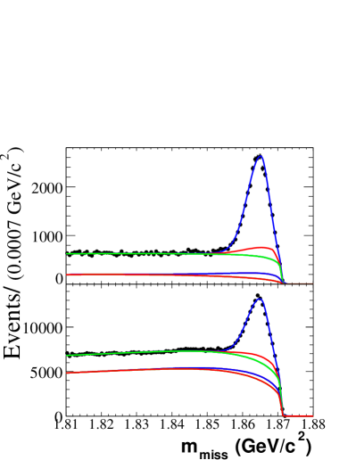
Figure 2: The $m_{\rm miss}$ distributions for on-resonance lepton-tagged (top) and kaon-tagged (bottom) data. The curves show, from bottom to top, the cumulative contributions of the continuum, peaking $B\kern 1.79993pt\overline{\kern-1.79993ptB}{}$, combinatoric $B\kern 1.79993pt\overline{\kern-1.79993ptB}{}$, $B\rightarrow D^{*\mp}\rho^{\pm}$, and $B\rightarrow D^{*\mp}\pi^{\pm}$ PDF components.

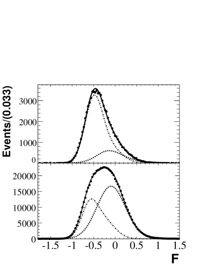
Figure 3: The $F$ distributions for on-resonance lepton-tagged (top) and kaon-tagged (bottom) data. The contributions of the $B\kern 1.79993pt\overline{\kern-1.79993ptB}{}$ (dashed-dotted line) and the continuum (dashed line) PDF components are overlaid, peaking at approximately $-0.6$ and $-0.1$, respectively. The total PDF is also overlaid.

The results of the signal region fit (fourth step) are summarized in Table 1, and the plots of the $\Delta t$ distributions for the data are shown in Fig. 4 for the lepton-tagged and the kaon-tagged events. The goodness of the fit has been verified with the Kolmogorov-Smirnov test and by comparing the likelihood obtained in the fit with the likelihood distribution of many parameterized MC experiments generated with the PDF’s obtained in the fit on the data. Fig. 5 shows the raw, time-dependent $C\!P$ asymmetry

$$A(\Delta t)={N_{s_{{}_{\rm t}}=1}(\Delta t)-N_{s_{{}_{\rm t}}=-1}(\Delta t)\over N_{s_{{}_{\rm t}}=1}(\Delta t)+N_{s_{{}_{\rm t}}=-1}(\Delta t)}.$$ (26)

In the absence of background and with high statistics, perfect tagging, and perfect $\Delta t$ measurement, $A(\Delta t)$ would be a sinusoidal oscillation with amplitude $a_{D^{*}\pi}$. For presentation purposes, the requirements $m_{\rm miss}>1.855$ ${\mathrm{\,Ge\kern-1.00006ptV\!/}c^{2}}$ and $F<0$ were applied to the data plotted in Figs. 4 and 5, in order to reduce the background. These requirements were not applied to the fit sample, so they do not affect our results.

The fitted values of $\Delta m$ reported in Table 1 are in good agreement with the world average $(0.502\pm 0.007)~{}{\rm\,ps}^{-1}$ ref:pdg2004 . The fitted values of the $B^{0}$ lifetime need to be corrected for a bias observed in the simulated samples, $\Delta\tau=\tau_{fit}-\tau_{gen}=(-0.03\pm 0.02)~{}{\rm\,ps}$ for the lepton-tag and $\Delta\tau=(-0.04\pm 0.02)~{}{\rm\,ps}$ for the kaon-tag events. After this correction, the measured lifetimes, $\tau(B^{0})=(1.48\pm 0.02\pm 0.02)~{}{\rm\,ps}$ and $\tau(B^{0})=(1.49\pm 0.01\pm 0.04)~{}{\rm\,ps}$ for the lepton-tag and kaon-tag, respectively, are in reasonable agreement with the world average $\tau(B^{0})=(1.536\pm 0.014)~{}{\rm\,ps}$ ref:pdg2004 . The correlation coefficients of $a_{D^{*}\pi}^{\ell}$ ($c_{D^{*}\pi}^{\ell}$) with $\Delta m$ and $\tau(B^{0})$ are $-0.021$ and 0.019 ($-0.060$ and $-0.056$).

Table 1: Results of the fit to the lepton- and kaon-tagged events in the signal region $1.845<m_{\rm miss}<1.880$ ${\mathrm{\,Ge\kern-1.00006ptV\!/}c^{2}}$. Errors are statistical only. See Sections III.6.2, III.6.3, and III.6.4 for the definitions of the symbols used in this table.

	Lepton tags		Kaon tags
Parameter description	Parameter	Value	Parameter	Value
Signal weak phase par.	$a_{{D^{*}\pi}}^{\ell}$	$-0.042\pm 0.019$	$a_{D^{*}\pi}^{K}$	$-0.025\pm 0.020$
			$b_{D^{*}\pi}^{K}$	$-0.004\pm 0.010$
	$c_{{D^{*}\pi}}^{\ell}$	$-0.019\pm 0.022$	$c_{D^{*}\pi}^{K}$	$-0.003\pm 0.020$
Signal $\Delta t$ PDF	$\Delta m_{{{D^{*}\pi}}}$	$0.518\pm 0.010$ ps-1	$\Delta m_{{{D^{*}\pi}}}$	$0.4911\pm 0.0076$ ps-1
	$\tau_{{{D^{*}\pi}}}$	$1.450\pm 0.017$ ps	$\tau_{{{D^{*}\pi}}}$	$1.449\pm 0.011$ ps
	$\omega_{{{D^{*}\pi}}}^{{\rm dir}}$	$0.010\pm 0.006$	$\omega_{{{D^{*}\pi}}}$	$0.2302\pm 0.0035$
			$\Delta\omega_{{{D^{*}\pi}}}$	$-0.0181\pm 0.0068$
	$\Delta\epsilon_{{D^{*}\pi}}$	$0.027\pm 0.010$	$\Delta\epsilon_{{D^{*}\pi}}$	$-0.0070\pm 0.0073$
Signal resolution function	$b^{n}_{{{D^{*}\pi}}}{{}^{{\rm cas}}}$	$-0.58\pm 0.16$
	$b^{w}_{{{D^{*}\pi}}}{{}^{{\rm cas}}}$	$0.23\pm 2.01$
	$b^{n}_{{{D^{*}\pi}}}{{}^{{\rm dir}}}$	$0.$ (fixed)	$b^{n}_{{{D^{*}\pi}}}$	$-0.255\pm 0.013$
	$b^{w}_{{{D^{*}\pi}}}{{}^{{\rm dir}}}$	$0.$ (fixed)	$b^{w}_{{{D^{*}\pi}}}$	$-2.07\pm 0.48$
	$f^{n}_{{{D^{*}\pi}}}{{}^{{\rm dir}}}$	$0.978\pm 0.008$	$f^{n}_{{{D^{*}\pi}}}$	$0.969\pm 0.007$
	$f^{o}_{{{D^{*}\pi}}}{{}^{{\rm dir}}}$	$0.$ (fixed)	$f^{o}_{{{D^{*}\pi}}}$	$0.000\pm 0.001$
	$s^{n}_{{{D^{*}\pi}}}{{}^{{\rm dir}}}$	$1.080\pm 0.033$	$s^{n}_{{{D^{*}\pi}}}$	$1.029\pm 0.023$
	$s^{w}_{{{D^{*}\pi}}}{{}^{{\rm dir}}}$	$5.76\pm 1.44$	$s^{w}_{{{D^{*}\pi}}}$	$4.35\pm 0.40$
Continuum $\Delta t$ PDF	$\tau_{{q\overline{q}}}$	1.26 $\pm$ 0.32 ps	$\tau_{{q\overline{q}}}$	$0.707\pm 0.048$ ps
	$\omega_{{q\overline{q}}}$	0.340 $\pm$ 0.009	$\omega_{{q\overline{q}}}^{\tau}$	$0.045\pm 0.022$
			$\omega_{{q\overline{q}}}^{\delta}$	$0.311\pm 0.006$
	$f^{\delta}_{q\overline{q}}$	0.815 $\pm$ 0.064	$f^{\delta}_{q\overline{q}}$	$0.820\pm 0.015$
Continuum resolution function	$b^{n}_{{q\overline{q}}}$	0.026 $\pm$ 0.048	$b^{n}_{{q\overline{q}}}$	0.017 $\pm$ 0.005
	$b^{w}_{{q\overline{q}}}$	$-0.39\pm$ 0.23	$b^{w}_{{q\overline{q}}}$	$-0.043\pm 0.043$
	$f^{n}_{{q\overline{q}}}$	0.65 $\pm$ 0.12	$f^{n}_{{q\overline{q}}}$	0.858 $\pm$ 0.014
	$f^{o}_{{q\overline{q}}}$	0.068 $\pm$ 0.014	$f^{o}_{{q\overline{q}}}$	0.018 $\pm$ 0.001
	$s^{n}_{{q\overline{q}}}$	0.929 $\pm$ 0.078	$s^{n}_{{q\overline{q}}}$	1.064 $\pm$ 0.008
	$s^{w}_{{q\overline{q}}}$	$1.81\pm 0.28$	$s^{w}_{{q\overline{q}}}$	2.267 $\pm$ 0.099

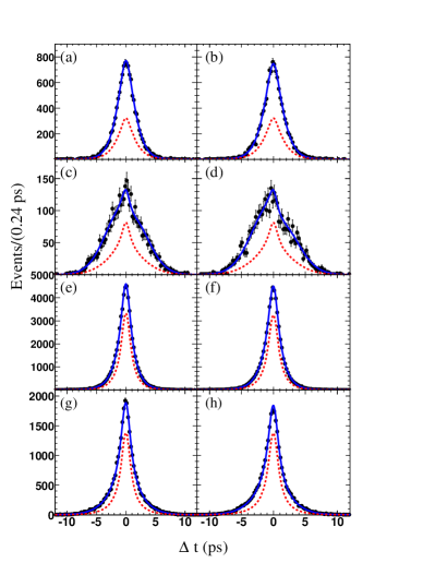
Figure 4: $\Delta t$ distributions for the lepton-tagged (a-d) and kaon-tagged (e-h) events separated according to the tagged flavor of $B_{\rm tag}$ and whether they were found to be mixed or unmixed: a,e) $B^{0}$ unmixed, b,f) $\kern 1.79993pt\overline{\kern-1.79993ptB}{}^{0}$ unmixed, c,g) $B^{0}$ mixed, d,h) $\kern 1.79993pt\overline{\kern-1.79993ptB}{}^{0}$ mixed. The solid curves show the PDF, calculated with the parameters obtained by the fit. The PDF for the total background is shown by the dashed curves.

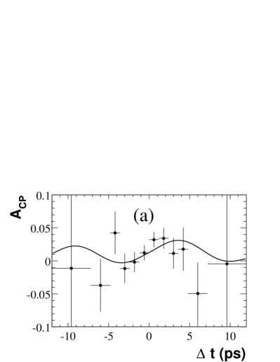
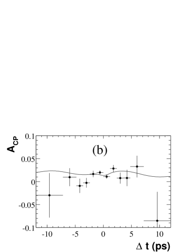
Figure 5: Raw asymmetry for (a) lepton-tagged and (b) kaon-tagged events. The curves represent the projections of the PDF for the raw asymmetry. A nonzero value of $a_{D^{*}\pi}$ would show up as a sinusoidal asymmetry, up to resolution and background effects. The offset from the horizontal axis is due to the nonzero values of $\Delta\epsilon_{{D^{*}\pi}}$ and $\Delta\omega_{{{D^{*}\pi}}}$.

V SYSTEMATIC STUDIES

The systematic errors are summarized in Table 2. Each item below corresponds to the item with the same number in Table 2.

• The statistical errors from the fit in Step 1 are propagated to the final fit. This also includes the systematic errors due to possible differences between the PDF line shape and the data points.

• The statistical errors from the $m_{\rm miss}$ sideband fit (Step 3) are propagated to the final fit (Step 4).

• The statistical errors from the Step 2 fits are propagated to the final fit.

• The statistical errors associated with the parameters obtained from MC are propagated to the final fit. In addition, the full analysis has been performed on a simulated sample to check for a possible bias in the weak phase parameters measured. No statistically significant bias has been found and the statistical uncertainty of this test has been assigned as a systematical error.

• The effect of uncertainties in the beam-spot size on the vertex constraint is estimated by increasing the beam spot size by 50$~{}\mu$m.

• The effect of the uncertainty in the measured length of the detector in the $z$ direction is evaluated by applying a 0.6% variation to the measured values of $\Delta t$ and $\sigma_{\Delta t}$.

• To evaluate the effect of possible misalignments in the SVT, signal MC events are reconstructed with different alignment parameters, and the analysis is repeated.

• The weak phase parameters of the $B\rightarrow D^{*\mp}\rho^{\pm}$, peaking, and combinatoric $B\kern 1.79993pt\overline{\kern-1.79993ptB}{}$ background are fixed to 0 in the fits. To study the effect of possible interference between $b\rightarrow u\bar{c}d$ and $b\rightarrow c\bar{u}d$ amplitudes in these backgrounds, their weak phase parameters are varied in the range $\pm 0.04$ and the Step-4 fit is repeated. We take the largest variation in each weak phase parameter as its systematic error.

• In the final fit, we take the values of the parameters of ${\cal T}^{\prime}_{\rm peak}$ from a fit to simulated peaking $B\kern 1.79993pt\overline{\kern-1.79993ptB}{}$ background events. The uncertainty due to this is evaluated by fitting the simulated sample, setting the parameters of ${\cal T}^{\prime}_{\rm peak}$ to be identical to those of ${\cal T}^{\prime}_{\rm comb}$.

• The uncertainty due to possible differences between the $\Delta t$ distributions for the combinatoric background in the $m_{\rm miss}$ sideband and signal region is evaluated by comparing the results of fitting the simulated sample with the ${\cal T}^{\prime}_{\rm comb}$ parameters taken from the sideband or the signal region.

• The ratio $f_{D^{*}\rho}/f_{D^{*}\pi}$ is varied by the uncertainty in the corresponding ratio of branching fractions, obtained from Ref. ref:pdg2004 .

Table 2: Systematic errors in $a_{D^{*}\pi}^{\ell}$ and $c_{D^{*}\pi}^{\ell}$ for lepton-tagged events and $a_{D^{*}\pi}^{K}$, $b_{D^{*}\pi}^{K}$, and $c_{D^{*}\pi}^{K}$ for kaon-tagged events.

Source	Error $(\times 10^{-2})$
	Lepton tags		Kaon tags
	$a_{D^{*}\pi}^{\ell}$	$c_{D^{*}\pi}^{\ell}$	$a_{D^{*}\pi}^{K}$	$b_{D^{*}\pi}^{K}$	$c_{D^{*}\pi}^{K}$
1. Step 1 fit	0.04	0.04	$0.10$	$0.04$	$0.04$
2. Sideband statistics	0.08	0.08	$0.40$	$0.12$	$0.44$
3. $f^{\rm miss}_{D^{*}\pi}$	0.02	0.02	$0.02$	negl.	negl.
4. $\rho_{D^{*}\pi}$	0.02	0.02	$0.02$	negl.	negl.
5. MC statistics	0.60	0.82	$0.68$	$0.34$	$0.70$
6. Beam spot size	0.10	0.10	$0.07$	$0.13$	$0.06$
7. Detector $z$ scale	0.03	0.03	$0.02$	negl.	$0.03$
8. Detector alignment	0.25	0.55	$0.25$	$0.13$	$0.41$
9. Combinatoric background weak phase par.	0.25	0.22	$0.80$	$0.56$	$0.72$
10. Peaking background weak phase par.	0.36	0.38	$0.29$	$0.17$	$0.27$
11. $D^{*}\rho$ weak phase par.	0.53	0.52	$0.57$	$0.58$	$0.58$
12. Peaking background	0.21	0.31	$0.21$	$0.41$	$0.31$
13. Signal region/sideband difference	negl.	negl.	$0.04$	$0.03$	$0.05$
14. $\cal B$($B\rightarrow D^{*\mp}\rho^{\pm}$)	0.17	0.33	$0.17$	$0.22$	$0.33$
Total systematic error	1.0	1.3	$1.4$	$1.0$	$1.5$
Statistical uncertainty	1.9	2.2	2.0	1.0	2.0

VI PHYSICS RESULTS

Summarizing the values and uncertainties of the weak phase parameters, we obtain the following results from the lepton-tagged sample:

$$a_{D^{*}\pi}^{\ell} = -0.042\pm 0.019\pm 0.010,$$

$$c_{D^{*}\pi}^{\ell} = -0.019\pm 0.022\pm 0.013.$$ (27)

The results from the kaon-tagged sample fits are

$$a_{D^{*}\pi}^{K} = -0.025\pm 0.020\pm 0.013,$$

$$b_{D^{*}\pi}^{K} = -0.004\pm 0.010\pm 0.010,$$

$$c_{D^{*}\pi}^{K} = -0.003\pm 0.020\pm 0.015.$$ (28)

Combining the results for lepton and kaon tags gives the amplitude of the time-dependent $C\!P$ asymmetry,

$$a_{D^{*}\pi} = 2{r^{*}}\sin(2\beta+\gamma)\cos\delta^{*}$$ (29)

$$= -0.034\pm 0.014\pm 0.009,$$

where the first error is statistical and the second is systematic. The systematic error takes into account correlations between the results of the lepton- and kaon-tagged samples coming from the systematic uncertainties related to detector effects, to interference between $b\rightarrow u\bar{c}d$ and $b\rightarrow c\bar{u}d$ amplitudes in the backgrounds and from $\cal B$($B\rightarrow D^{*\mp}\rho^{\pm}$). This value of $a_{D^{*}\pi}$ deviates from zero by 2.0 standard deviations.

Previous results of time-dependent $C\!P$ asymmetries related to $2\beta+\gamma$ appear in Ref. ref:run1-2 ; ref:others . This measurement supersedes the results of the partial reconstruction analysis reported in Ref. ref:run1-2 and improves the precision on $a_{D^{*}\pi}$ and $c_{D^{*}\pi}$ with respect to the average of the published results.

We use a frequentist method, inspired by Ref. ref:Feldman , to set a constraint on $2\beta+\gamma$. To do this, we need a value for the ratio ${r^{*}}$ of the two interfering amplitudes. This is done with two different approaches.

In the first approach, to avoid any assumptions on the value of ${r^{*}}$, we obtain the lower limit on $|\sin(2\beta+\gamma)|$ as a function of ${r^{*}}$.

We define a $\chi^{2}$ function that depends on ${r^{*}}$, $2\beta+\gamma$, and $\delta^{*}$:

$$\chi^{2}({r^{*}},2\beta+\gamma,\delta^{*})=\sum_{j,k=1}^{3}\Delta x_{j}V^{-1}_{jk}\Delta x_{k},$$ (30)

where $\Delta x_{j}$ is the difference between the result of our measurement of $a_{D^{*}\pi}^{K}$, $a_{D^{*}\pi}^{\ell}$, or $c_{D^{*}\pi}^{\ell}$ (Eqs. (28) and (27)) and the corresponding theoretical expressions given by Eq. (12). We fix ${r^{*}}$ to a trial value $r^{0}$. The measurements of $b_{D^{*}\pi}^{K}$ and $c_{D^{*}\pi}^{K}$ are not used in the fit, since they depend on the unknown values of $r^{\prime}$ and $\delta^{\prime}$. The measurement error matrix $V$ is nearly diagonal, and accounts for correlations between the measurements due to correlated statistical and systematic uncertainties. We minimize $\chi^{2}$ as a function of $2\beta+\gamma$ and $\delta^{*}$, and obtain $\chi^{2}_{min}$, the minimum value of $\chi^{2}$.

In order to compute the confidence level for a given value $x$ of $2\beta+\gamma$, we perform the following procedure:

1. We fix the value of $2\beta+\gamma$ to $x$ and minimize $\chi^{2}$ as a function of $\delta^{*}$. We define $\chi^{\prime 2}_{min}(x)$ to be the minimum value of the $\chi^{2}$ in this fit, and $\delta^{*}_{toy}$ to be the fitted value of $\delta^{*}$. We define $\Delta\chi^{2}(x)\equiv\chi^{\prime 2}_{min}(x)-\chi^{2}_{min}$.

2. We generate many parameterized MC experiments with the same sensitivity as the data sample, taking into account correlations between the observables, expressed in the error matrix $V$ of Eq. (30). To generate the observables $a_{D^{*}\pi}^{K}$, $a_{D^{*}\pi}^{\ell}$, and $c_{D^{*}\pi}^{\ell}$, we use the values $(2\beta+\gamma)=x$, ${r^{*}}=r^{0}$ and $\delta^{*}=\delta^{*}_{toy}$. For each experiment we calculate the value of $\Delta\chi^{2}(x)$, computed with the same procedure used for the experimental data.

3. We interpret the fraction of these experiments for which $\Delta\chi^{2}(x)$ is smaller than $\Delta\chi^{2}(x)$ in the data to be the confidence level (CL) of the lower limit on $(2\beta+\gamma)=x$.

The resulting 90% CL lower limit on $|\sin(2\beta+\gamma)|$ as a function of ${r^{*}}$ is shown in Fig. 6. The $\chi^{2}$ function is invariant under the transformation $2\beta+\gamma\rightarrow\pi/2+\delta^{*}$ and $\delta^{*}\rightarrow\pi/2-2\beta+\gamma$. The limit shown in Fig. 6 is always the weaker of these two possibilities.

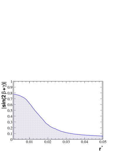
Figure 6: Lower limit on $|\sin(2\beta+\gamma)|$ at 90% CL as a function of ${r^{*}}$, for ${r^{*}}>0.001$.

In the second approach, we estimate ${r^{*}}$ as originally proposed in Ref. ref:book , and assume SU(3) flavor symmetry. With this assumption, ${r^{*}}$ can be estimated from the Cabibbo angle $\theta_{C}$, the ratio of branching fractions ${\cal B}(B^{0}\rightarrow{D^{*}}_{s}^{+}\pi^{-})/{\cal B}(B^{0}\rightarrow{D^{*}}^{-}\pi^{+})=(5.4^{+3.4}_{-3.7}\pm 0.7)\times 10^{-3}$ ref:Dspi , and the ratio of decay constants $f_{D^{*}_{s}}/f_{D^{*}}=1.10\pm 0.02$ ref:dec-const ,

$${r^{*}} = \sqrt{\frac{{\cal B}(B^{0}\rightarrow{D^{*}}_{s}^{+}\pi^{-})}{{\cal B}(B^{0}\rightarrow{D^{*}}^{-}\pi^{+})}}\,\frac{f_{D^{*}}}{f_{D^{*}_{s}}}\,\tan(\theta_{C}),$$ (31)

yielding the measured value

$$r^{*\rm meas}=0.015^{+0.004}_{-0.006}.$$ (32)

This value depends on the value of ${\cal B}(D_{s}^{+}\rightarrow\phi\pi^{+})$, for which we use our recent measurement ref:phipi .

Equation (31) has been obtained with two approximations. In the first approximation, the exchange diagram amplitude $E$ contributing to the decay $B^{0}\rightarrow{D^{*}}^{+}\pi^{-}$ has been neglected and only the tree-diagram amplitude $T$ has been considered. Unfortunately, no reliable estimate of the exchange term for these decays exists. The only decay mediated by an exchange diagram for which the rate has been measured is the Cabibbo-allowed decay $B^{0}\rightarrow D_{s}^{-}K^{+}$. The average of the BABAR and Belle branching fraction measurements ref:Dspi ; ref:belledsk is $(3.8\pm 1.0)\times 10^{-5}$. This yields the approximate ratio ${\cal B}(B^{0}\rightarrow D_{s}^{-}K^{+})/{\cal B}(B^{0}\rightarrow D^{-}\pi^{+})\sim 10^{-2}$, which confirms that the exchange diagrams are strongly suppressed with respect to the tree diagrams. Detailed analyses ref:topolo of the $B\rightarrow D\pi$ and $B\rightarrow D^{*}\pi$ decays in terms of the topological amplitudes conclude that $|E^{\prime}/T^{\prime}|=0.12\pm 0.02$ for $B^{0}\rightarrow D^{-}\pi^{+}$ and $|\bar{E}/\bar{T}|<0.10$ for $B^{0}\rightarrow{D^{*}}^{-}\pi^{+}$ decays, where $E^{\prime}$, $\bar{E}$ and $T^{\prime}$, $\bar{T}$ are the exchange and tree amplitudes for these Cabibbo-allowed decays. We assume that a similar suppression holds for the Cabibbo-suppressed decays considered here.

The second approximation involves the use of the ratio of decay constants $f_{D^{*}}/f_{D^{*}_{s}}$ to take into account SU(3) breaking effects and assumes factorization. We attribute a 30% relative error to the theoretical assumptions involved in obtaining the value of ${r^{*}}$ of Eq. (32), and use it as described below.

We add to the $\chi^{2}$ of Eq. (30) the term $\Delta^{2}({r^{*}})$ that takes into account both the Gaussian experimental errors of Eq. (32) and the 30% theoretical uncertainty according to the prescription of Ref. Hocker:2001xe :

$$\Delta^{2}({r^{*}})=\left\{\begin{matrix}\left(\dfrac{{r^{*}}-1.3\,r^{*\rm meas}}{0.004}\right)^{2}&,&\xi_{r^{*}}>0.3&,\\[14.22636pt] 0&,&\left|\xi_{r^{*}}\right|\leq 0.3&,\\[5.69054pt] \left(\dfrac{{r^{*}}-0.7\,r^{*\rm meas}}{0.006}\right)^{2}&,&\xi_{r^{*}}<-0.3&,\end{matrix}\right.$$ (33)

where $\xi_{r^{*}}\equiv{({r^{*}}-r^{*\rm meas})/r^{*\rm meas}}$.

To obtain the confidence level we have repeated the procedure described above with the following changes. To compute $\chi^{2}_{min}$ we minimize $\chi^{2}$ as a function of $2\beta+\gamma$, ${r^{*}}$ and $\delta^{*}$. The value $\chi^{\prime 2}_{min}(x)$ is obtained minimizing $\chi^{2}$ as a function of ${r^{*}}$ and $\delta^{*}$, having fixed $2\beta+\gamma$ to a given value $x$. We define $\delta^{*}_{toy}$ and ${r^{*}}_{toy}$ to be the fitted value of $\delta^{*}$ and ${r^{*}}$ in this fit. To generate the observables $a_{D^{*}\pi}^{K}$, $a_{D^{*}\pi}^{\ell}$, and $c_{D^{*}\pi}^{\ell}$ in the parameterized MC experiments, we use the values $(2\beta+\gamma)=x$, ${r^{*}}={r^{*}}_{toy}$ and $\delta^{*}=\delta^{*}_{toy}$.

The confidence level as a function of $|\sin(2\beta+\gamma)|$ is shown in Fig. 7. We set the lower limits $|\sin(2\beta+\gamma)|>0.62~{}(0.35)$ at 68% (90%) CL. The implied probability contours for the apex of the unitarity triangle, parameterized in terms of $\bar{\rho}$ and $\bar{\eta}$ defined in Ref. ref:wolfen , appear in Fig. 8.

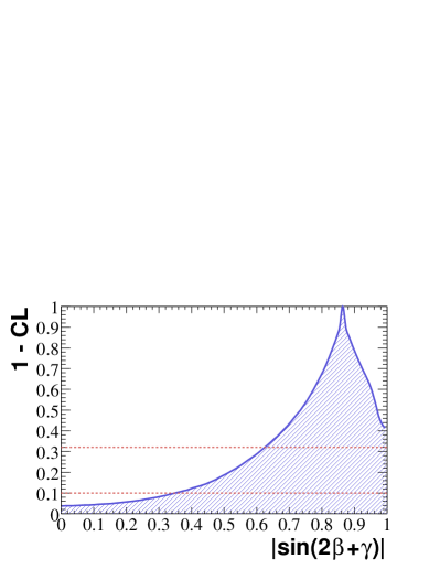
Figure 7: The shaded region denotes the allowed range of $|\sin(2\beta+\gamma)|$ for each confidence level. The horizontal lines show, from top to bottom, the 68% and 90% CL.

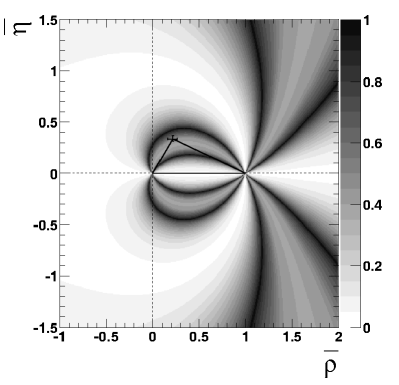
Figure 8: Contours of constant probability (color-coded in percent) for the position of the apex of the unitary triangle to be inside the contour, based on the results of Fig. 7. The cross represents the value and errors on the position of the apex of the unitarity triangle from the CKMFitter fit using the “ICHEP04” results excluding this measurement Hocker:2004 .

VII SUMMARY

We present a measurement of the time-dependent $C\!P$ asymmetries in a sample of partially reconstructed $B^{0}\rightarrow D^{*}{{}^{+}}\pi^{-}$ events. In particular, we have measured the parameters related to $2\beta+\gamma$ to be

$$a_{D^{*}\pi} = 2{r^{*}}\sin(2\beta+\gamma)\cos\delta^{*}$$ (34)

$$= -0.034\pm 0.014\pm 0.009$$

and

$$c_{D^{*}\pi}^{\ell} = 2{r^{*}}\cos(2\beta+\gamma)\sin\delta^{*}$$ (35)

$$= -0.019\pm 0.022\pm 0.013,$$

where the first error is statistical and the second is systematic. We extract limits as a function of the ratio ${r^{*}}$ of the $b\rightarrow u\overline{c}d$ and $b\rightarrow c\overline{u}d$ decay amplitudes. With some theoretical assumptions, we interpret our results in terms of the lower limits $|\sin(2\beta+\gamma)|>0.62~{}(0.35)$ at 68% (90%) CL.

VIII Acknowledgments

We are grateful for the extraordinary contributions of our PEP-II colleagues in achieving the excellent luminosity and machine conditions that have made this work possible. The success of this project also relies critically on the expertise and dedication of the computing organizations that support BABAR. The collaborating institutions wish to thank SLAC for its support and the kind hospitality extended to them. This work is supported by the US Department of Energy and National Science Foundation, the Natural Sciences and Engineering Research Council (Canada), Institute of High Energy Physics (China), the Commissariat à l’Energie Atomique and Institut National de Physique Nucléaire et de Physique des Particules (France), the Bundesministerium für Bildung und Forschung and Deutsche Forschungsgemeinschaft (Germany), the Istituto Nazionale di Fisica Nucleare (Italy), the Foundation for Fundamental Research on Matter (The Netherlands), the Research Council of Norway, the Ministry of Science and Technology of the Russian Federation, and the Particle Physics and Astronomy Research Council (United Kingdom). Individuals have received support from CONACyT (Mexico), the A. P. Sloan Foundation, the Research Corporation, and the Alexander von Humboldt Foundation.

References

(1) N. Cabibbo, Phys. Rev. Lett. 10,
531 (1963);
M. Kobayashi and T. Maskawa,
Prog. Theoret. Phys. 49, 652 (1973).
(2)
I. Dunietz, Phys. Lett. B 427, 179 (1998).
(3)BABAR Collaboration, B. Aubert et al., Phys. Rev. Lett.
89, 201802 (2002);
BABAR Collaboration, B. Aubert et al., hep-ex/0408127, submitted to
Phys. Rev. Lett.;
Belle Collaboration, K. Abe et al.,
Phys. Rev. D 66, 071102 (2002).
(4)
L. Wolfenstein, Phys. Rev. Lett. 51, 1945 (1983).
(5)BABAR Collaboration, B. Aubert et al.,
Phys. Rev. Lett. 92, 251802 (2004).
(6)BABAR Collaboration,
B. Aubert et al.,
Phys. Rev. D 67, 091101 (2003).
(7)
GEANT4 Collaboration, S. Agostinelli et al.,
Nucl. Instrum. Meth. A 506, 250 (2003).
(8)BABAR Collaboration, B. Aubert et al.,
Nucl. Instrum. Meth. A 479, 1 (2002).
(9)
Particle Data Group,
S. Eidelman et al., Phys. Lett. B 592, 1 (2004).
(10) G. Fox and S. Wolfram, Phys. Rev. Lett. 41,
1581 (1978).
(11) R. A. Fisher, Annals of Eugenics 7, 179 (1936);
M.S. Srivastava and E.M. Carter, “An Introduction to Applied
Multivariate Statistics”, North Holland, Amsterdam (1983).
(12)
ARGUS Collaboration, H. Albrecht et al.,
Phys. Lett. B 254,
288 (1991).
(13) O. Long,
M. Baak, R.N. Cahn, and D. Kirkby,
Phys. Rev. D 68, 034010 (2003).
(14)BABAR Collaboration, B. Aubert et al.,
Phys. Rev. Lett. 92, 251801 (2004);
Belle Collaboration, T. Sarangi et al.,
Phys. Rev. Lett. 93, 031802 (2004).
(15) G. Feldman and R. Cousins, Phys. Rev. D 57,
3873 (1998).
(16)BABAR Collaboration, B. Aubert et al.,
Phys. Rev. Lett. 90, 181803 (2003).
(17) D. Becirevic, Nucl. Phys. Proc. Suppl. 94,
337 (2001).
(18)BABAR Collaboration, B. Aubert et al.,
hep-ex/0408040, submitted to Phys. Rev. Lett.
(19)
Belle Collaboration, P. Krokovny et al.,
Phys. Rev. Lett. 89, 231804 (2002).
(20)
C.W. Chiang and J.L. Rosner, Phys. Rev. D 67, 074013 (2003);
C.S. Kim, S. Oh, and C. Yu, hep-ph/0412418.
(21)
A. Höcker et al.,
Eur. Phys. J. C 21, 225 (2001).
(22)
J. Charles et al. (CKMFitter Group), hep-ph/0406184 (to appear
in Eur. Phys. J. C).