Abstract

We present the first measurement of the $A_{2}$ and $A_{3}$ angular coefficients of the $W$ boson produced in proton-antiproton collisions. We study $W\rightarrow e\nu_{e}$ and $W\rightarrow\mu\nu_{\mu}$ candidate events produced in association with at least one jet at CDF, during Run Ia and Run Ib of the Tevatron at $\sqrt{s}$=1.8 TeV. The corresponding integrated luminosity was 110 pb^-1. The jet balances the transverse momentum of the $W$ and introduces QCD effects in $W$ boson production. The extraction of the angular coefficients is achieved through the direct measurement of the azimuthal angle of the charged lepton in the Collins-Soper rest-frame of the $W$ boson. The angular coefficients are measured as a function of the transverse momentum of the $W$ boson. The electron, muon, and combined results are in good agreement with the Standard Model prediction, up to order $\alpha_{s}^{2}$ in QCD.

I Introduction

Measurements of the $W$ boson differential cross section, as a function of energy and direction, provide information about the nature of both the underlying electroweak interaction, and the effects of chromodynamics (QCD). This differential cross section can be expressed us a function of the helicity cross sections of the $W$, allowing us to study the $W$ polarization and associated asymmetries. Because of the difficulties in fully reconstructing a $W$ boson in three-dimensions at a hadron collider, the complete angular distribution of the $W$ has not been determined yet. In this paper we present the first measurement of two of the four significant leading angular coefficients of the $W$ boson produced at a hadron collider.

The total differential cross section for $W$ boson production in a hadron collider is given by

$$\frac{d{\sigma}}{d(p_{T}^{W})^{2}dyd\cos{\theta}d\phi} = \frac{3}{16\pi}\frac{d\sigma^{u}}{d(p_{T}^{W})^{2}dy}[(1+\cos^{2}{\theta})$$ (1)

$$+ \frac{1}{2}A_{0}(1-3\cos^{2}{\theta})+A_{1}\sin{2\theta}\cos{\phi}$$

$$+ \frac{1}{2}A_{2}\sin^{2}{\theta}\cos{2\phi}+A_{3}\sin{\theta}\cos{\phi}$$

$$+ A_{4}\cos{\theta}+A_{5}\sin^{2}\theta\sin 2\phi$$

$$+ A_{6}\sin{2\theta}\sin{\phi}+A_{7}\sin{\theta}\sin{\phi}]$$

where $p_{T}^{W}$ and $y$ are the transverse momentum and the rapidity of the $W$ in the laboratory frame, and $\theta$ and $\phi$ are the polar and azimuthal angles of the charged lepton from $W$ boson decay in the Collins-Soper (CS) frame Mirkes (1992). The factors $A_{i}(p_{T}^{W},y)$ are the angular coefficients of the $W$ boson, which are ratios of the helicity cross sections of the $W$ and its total unpolarized cross section $d\sigma^{u}/d(p_{T}^{W})^{2}dy$. The CS frame Collins and Soper (1977) is the rest-frame of the $W$ with a $z$-axis that bisects the angle between the proton direction and the direction opposite that of the antiproton (Figure 1), and it is used because in this frame we can in principle exactly reconstruct the azimuthal angle $\phi$ and the polar quantity $|\cos{\theta}|$. Our ignorance of the $W$ boson longitudinal momentum, which is due to our inability to measure the longitudinal momentum of the neutrino, only introduces a two-fold ambiguity on the sign of $\cos\theta$. It is common to integrate Equation (1) over $y$ and study the variation of the angular coefficients as a function of $p_{T}^{W}$.

To study the angular distribution of the $W$ we must choose a particular charge for the boson. In this paper we consider the $W^{-}$ bosons; the $W^{+}$ bosons in our samples are $CP$ transformed to be treated as $W^{-}$ bosons. The angular coefficients for the $W^{+}$ are obtained by $CP$ transforming Equation (1) foo (a).

If the $W$ is produced with no transverse momentum, it is polarized along the beam axis, due to the V-A nature of the weak interactions and helicity conservation. In that case $A_{4}$ is the only non-zero coefficient. If only valence quarks contributed to $W$ production, $A_{4}$ would equal 2, and the angular distribution given by Equation (1) would be $\sim(1+\cos\theta)^{2}$, a result that was first verified by the UA1 experiment Albajar et al. (1989).

If the $W$ is produced with non-negligible transverse momentum, balanced by the associated production of jets, the rest of the angular coefficients are present, and the cross section depends on the azimuthal angle $\phi$ as well. The last three angular coefficients $A_{5}$, $A_{6}$, and $A_{7}$ are non-zero only if gluon loops are present in the production of the $W$ boson. Hence, in order to study all the angular coefficients and associated helicity cross sections of the $W$ boson in a hadron collider, we must consider the production of the $W$ with QCD effects up to order $\alpha_{s}^{2}$.

The importance of the determination of the $W$ angular coefficients is discussed in Mirkes and Ohnemus (1994), and summarized here. It allows us to measure for the first time the full differential cross section of the $W$ and study its polarization, since the angular coefficients are directly related to the helicity cross sections. It also helps us verify the QCD effects in the production of the $W$ up to order $\alpha_{s}^{2}$. For example, according to the Standard Model (SM), $A_{2}$ is not equal to $A_{0}$ only if the effects of gluon loops are taken into account. In addition, $A_{3}$ is only affected by the gluon-quark interaction and its measurement can be used to constrain the gluon parton distribution functions. Moreover, the next-to-leading order angular coefficients $A_{5}$, $A_{6}$, and $A_{7}$ are $P$-odd and $T$-odd and may play an important role in direct $CP$ violation effects in $W$ production and decay Hagiwara et al. (1984). Finally, quantitative understanding of the $W$ angular distribution could be used to test new theoretical models and to facilitate new discoveries.

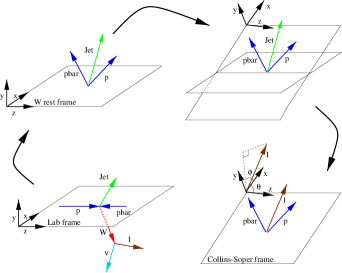
Figure 1: Transforming from the laboratory frame to the Collins-Soper frame. We first boost to the $W$ rest-frame, then rotate the $x-z$ plane so that it coincides with the $p$-$\bar{p}$ plane. Finally we rotate the frame around the $y$-axis so that the $z$-axis bisects the angle between $\vec{p}$ and $-\vec{\bar{p}}$. The positive $y$ axis is selected to have the same direction as $\vec{p}_{\rm{CS}}\times\vec{\bar{p}}_{\rm{CS}}$.

In this paper we present the first measurement of the $A_{2}$ and $A_{3}$ angular coefficients of the $W$ boson. These coefficients fully describe the azimuthal differential cross section of the $W$ boson, and they are two of the four significant coefficients that describe the total differential cross section of the $W$, given that $A_{1}$ and the next-to-leading order angular coefficients have considerably lower values Mirkes and Ohnemus (1994); Strologas and Errede (2005). This measurement is accomplished using the azimuthal angle of the charged lepton in the CS $W$ rest-frame Strologas (2002), and is presented as a function of the transverse momentum of the $W$ boson. The CS polar angle analysis is more sensitive to the $A_{0}$ and $A_{4}$ angular coefficients (see Abbott et al. (2001); Acosta et al. (2004) for a measurement of $A_{0}$). Because Equation (1) arises solely from quantum field theory, without input from any specific theoretical model of $W$ boson production, our experimental results are thus model-independent.

II The CDF detector and event selection

II.1 The CDF detector

The CDF detector is described in detail in Abe et al. (1988). It is a general purpose detector of charged leptons, hadrons, jets, and photons, produced from proton-antiproton collisions at the Tevatron accelerator at Fermilab. The $W$ and $Z$ bosons are detected through their decay leptons, while the transverse momentum of the neutrinos is estimated from the missing transverse energy of the events ($E_{T}\!\!\!\!\!\!\!/\,\,\,\,\,\,$).

The $z$-axis of the detector coincides with the direction of the proton beam and defines the polar angle $\theta_{\rm lab}$ in the laboratory frame. The $y$-axis points vertically upward and the $x$-axis is in the horizontal plane, so as to form a right-handed coordinate system. The pseudorapidity, $\eta_{\rm lab}=-\ln[\tan(\theta_{\rm lab}/2)]$, and the azimuthal angle $\phi_{\rm lab}$ are used to specify detector physical areas.

The tracking system of CDF consists of the silicon vertex detector (SVX), the vertex time projection chamber (VTX) and the central tracking chamber (CTC), all immersed in a 1.4 T magnetic field produced by a superconducting solenoid of length 4.8 m and radius 1.5 m. The SVX, a four layer silicon micro-strip vertex detector, is located immediately outside the beampipe. It is used to find secondary vertices and provides the impact parameter of tracks in the transverse $r-\phi_{\rm lab}$ plane. The VTX, located outside the SVX, is a vertex time projection chamber that provides $r-z$ tracking information up to a radius of 22 cm and pseudorapidity $|\eta_{\rm lab}|\leq 3.5$. It measures the $z$-position of the primary vertex. Finally, surrounding the SVX and the VTX is the CTC, a 3.2 m long cylindrical drift chamber containing 84 layers of sense wires arranged in five superlayers of axial wires and four superlayers of stereo wires. The axial superlayers have 12 radially separated layers of sense wires, parallel to the $z$-axis, that measure the $r-\phi_{\rm lab}$ position of the tracks. The stereo superlayers have six layers of sense wires with alternate $\sim\pm 3^{\circ}$ stereo angles with respect to the beamline, and measure a combination of $r-\phi_{\rm lab}$ and $z$ information. The stereo and axial data are combined to reconstruct the 3-dimensional track. The CTC covers the pseudorapidity interval $|\eta_{\rm lab}|<1.0$ and transverse momentum $p_{T}\geq 0.4$ GeV uni . The combined momentum resolution of the tracking system is $\delta p_{T}/p_{T}=\sqrt{(0.0009p_{T})^{2}+(0.0066)^{2}}$, where $p_{T}$ is the transverse momentum in GeV.

The solenoid is surrounded by sampling calorimeters used to measure the electromagnetic and hadronic energy of electrons, photons, and jets. The calorimeters cover the pseudorapidity range $|\eta_{\rm lab}|\leq 4.2$ and the azimuthal angle range $0\leq\phi_{\rm lab}\leq 2\pi$. They are segmented in $\eta_{\rm lab}-\phi_{\rm lab}$ towers pointing to the nominal interaction point at the center of the detector. The tower granularity is ($\Delta\eta_{\rm lab}\times\Delta\phi_{\rm lab})=(0.1\times 15^{\circ}$) in the central region ($0\leq|\eta_{\rm lab}|\leq 1.1$) and ($0.1\times 5^{\circ}$) in the plug ($1.1<|\eta_{\rm lab}|\leq 2.4$) and forward ($2.4<|\eta_{\rm lab}|\leq 4.2$) regions. Each region has an electromagnetic calorimeter (CEM in the central region, PEM in the plug region, and FEM in the forward region) followed by a hadron calorimeter at larger radius from the beam (CHA, PHA, and FHA respectively). The central calorimeters are segmented in 24 wedges per each half of the detector ($-1.1\leq\eta_{\rm lab}\leq 0$ and $0\leq\eta_{\rm lab}\leq 1.1$). The CEM is an 18 radiation length lead-scintillator stack with a position resolution of 2 mm and an energy resolution of $\delta E_{T}/E_{T}=\sqrt{(13.5\%/\sqrt{E_{T}})^{2}+(2\%)^{2}}$, where $E_{T}$ is the transverse energy in GeV. Located six radiation lengths deep inside the CEM calorimeter (184 cm from the beamline), proportional wire chambers (CES) with additional cathode strip read-out provide shower position measurements in the $z$ and $r-\phi_{\rm lab}$ directions. The central hadron calorimeter (CHA) is an iron-scintillator stack which is 4.5 interaction lengths thick and provides energy measurement with a resolution of $\delta E_{T}/E_{T}=\sqrt{(50\%/\sqrt{E_{T}})^{2}+(3\%)^{2}}$, where $E_{T}$ is the transverse energy in GeV.

The central muon system consists of three components and is capable of detecting muons with transverse momentum $p_{T}\geq 1.4$ GeV and pseudorapidity $|\eta_{\rm lab}|<1.0$. The Central Muon Chambers (CMU) cover the region $|\eta_{\rm lab}|<0.6$ and consist of four layers of planar drift chambers outside the hadron calorimeter, allowing the reconstruction of the muons which typically pass the five absorption lengths of material. Outside the CMU there are three additional absorption lengths of material (0.6 m of steel) followed by four layers of drift chambers, the Central Muon Upgrade (CMP). The CMP chambers cover the same pseudorapidity region as the CMU, and they were introduced to limit the background caused from punch-through pions. Finally, the Central Muon Extension chambers (CMX) cover the region $0.6\leq\eta_{\rm lab}\leq 1.0$. These drift chambers are sandwiched between scintillators (CSX). Depending on the incident angle, particles have to penetrate six to nine absorption lengths of material to be detected in the CMX. The particle candidate stub provided by the muon system is matched with a track from the CTC in order to successfully reconstruct a muon.

II.2 The CDF triggers

CDF has a three-level trigger system designed to select events that can contain electrons, muons, jets, and $E_{T}\!\!\!\!\!\!\!/\,\,\,\,\,\,$. The first two levels are implemented in hardware, while the third is a software trigger which uses a version of the offline reconstruction software optimized for speed and implemented by a CPU farm.

At level-1, electrons were selected by the presence of an electromagnetic trigger tower with energy above 6 GeV (Run Ia) or 8 GeV (Run Ib), where one trigger tower consisted of two adjacent physical towers (in pseudorapidity). Muons were selected by the presence of a track stub in the CMU or CMX, where there was also signal in the CMP.

At level-2, electrons satisfied one of several triggers. In Run Ia, the event passed the trigger if the energy cluster in the CEM was at least 9 GeV with a seed tower of at least 7 GeV, and a matching track with $p_{T}>9.2$ GeV was found by the Central Fast Tracker (CFT), the fast hardware processor that matched CTC tracks in the $r-\phi_{\rm lab}$ plane with signals in the calorimeters and muon chambers. It also passed the trigger if there was an isolated cluster in the CEM calorimeter of at least 16 GeV. The most common Run Ib level-2 electron trigger requires the existence of a cluster in the CEM with at least 16 GeV and the existence of a matching track in the CFT with $p_{T}>12$ GeV. The muon trigger at level-2 required a track of at least 9 GeV (Run Ia) or 12 GeV (Run Ib) that matched a CMX stub (CMX triggers), both CMU and CMP stubs (CMUP triggers), or a CMU stub but no CMP stub (CMNP triggers).

At level-3, reconstruction programs performed 3-dimensional track reconstruction. In the Run Ia level-3 electron trigger, most of the accepted events passed the requirement that the CEM cluster had $E_{T}>18$ GeV, and was associated with a track of $p_{T}>13$ GeV. The transverse energy of the cluster is defined as $E_{T}=E\sin\theta$, where $E$ is the total energy deposited in the CEM, and $\theta$ is the polar angle measured from the event vertex to the centroid of the cluster. Cuts were applied on the shape of the electron shower profile and the energy deposition patterns. In the Run Ib level-3 electron trigger, CEM $E_{T}>18$ GeV and CFT $p_{T}>13$ GeV requirements were applied. The muon trigger at level-3 required that the CFT transverse momentum was greater than 18 GeV, the energy deposited in the hadron calorimeter was less than 6 GeV, the energy deposited in the electromagnetic calorimeter was less than 2 GeV, and the extrapolated CTC track was no more than 2 centimeters away from the muon stub in the CMU chambers and 5 centimeters in the CMP or CMX chambers in the $x$ direction. Events that pass the level-3 trigger were recorded to tape for offline analysis.

II.3 The datasets

The events passing the three levels of our trigger system constitute the inclusive high-$p_{T}$ electron and muon data samples. We apply kinematic and lepton identification cuts, described in Sections II.3.1 and II.3.2 to obtain the inclusive $W$ electron and muon datasets respectively. Using these datasets we arrive at the $W$+jet datasets by applying the jet selection cuts described in Section II.3.3.

II.3.1 Inclusive $W$ Electron Selection

After passing the three levels of trigger requirements, the following event selection cuts are applied to the inclusive electron data sample:

$\bullet$ The event must belong to a good run.

$\bullet$ $E_{T}^{e}\geq$ 20 GeV,
where $E_{T}^{e}$ is the transverse energy of the CEM cluster, corrected for differences in response, non-linearities, and time-dependent changes.

$\bullet$ $|\eta_{\rm lab}^{e}|\leq 1$,
where $\eta_{\rm lab}^{e}$ is the pseudorapidity of the electron.

$\bullet$ The electron must fall in a fiducial part of the CEM calorimeter.

$\bullet$ ISO(0.4)$\equiv E_{\Delta R=0.4}^{\rm Excess}/E_{T}^{\rm cluster}<0.1$,
where $E_{\Delta R=0.4}^{\rm Excess}$ is the excess transverse energy in a cone of size $\Delta R=\sqrt{(\Delta\phi_{\rm lab})^{2}+(\Delta\eta_{\rm lab})^{2}}$ centered on the direction of the electromagnetic cluster, and $E_{T}^{\rm cluster}$ is the transverse energy of that cluster.

$\bullet$ $E^{\rm HAD}/E^{\rm EM}<0.055+0.00045E^{e}$,
where $E^{\rm HAD}$ is the energy deposited in the hadron calorimeter, and $E^{\rm EM}$ is the energy deposited in the electromagnetic calorimeter.

$\bullet$ $L_{\rm SHR}\equiv 0.14\sum_{i}\frac{E_{i}^{\rm meas}-E_{i}^{\rm exp}}{\sqrt{(0.14)^{2}E^{\rm meas}+(\Delta{E_{i}^{\rm exp}})^{2}}}<0.2$,
where $L_{\rm SHR}$ is the lateral shower profile, $E_{i}^{\rm meas}$ is the energy measured in the $i^{\rm{th}}$-tower adjacent to the seed tower, $E_{i}^{\rm exp}$ is the expectation for the energy in that tower, $\Delta{E_{i}^{\rm exp}}$ is the uncertainty on the expected energy, and $0.14\sqrt{E^{\rm meas}}$ is the uncertainty in the measurement of the cluster energy.

$\bullet$ $\chi^{2}_{\rm CES}<10$.
We measure the shower profile along the z direction using the CES strips and the shower profile along the x direction using the CES wires. By comparing the measured x-shape and z-shape to the ones determined from test-beam studies we extract the chi-squared quantities for the two directions. The chi-squared we use is the average of the two.

$\bullet$ $0.5\leq E^{\rm e}/p^{\rm e}\leq 2.0$,
where $E^{\rm e}$ is the corrected energy of the electron, and $p^{\rm e}$ is the beam-constrained momentum of the electron, i.e., the momentum determined when the fit trajectory of the CTC hits is constrained to pass through the beam line.

$\bullet$ $|\Delta X|<1.5$ cm and $|\Delta Z|<3.0$ cm,
where $\Delta X$ and $\Delta Z$ are the difference in the $x$ and $z$ directions respectively, between the extrapolated CTC track and the CES position of the shower.

$\bullet$ $|Z_{\rm VTX}|\leq 60$ cm,
where $Z_{\rm VTX}$ is the $z$ position of the primary vertex.

$\bullet$ Photon conversions are removed.

We next apply the following cuts:

$\bullet$ $\mbox{$E_{T}\!\!\!\!\!\!\!/\,\,\,\,\,\,$}>20$ GeV,
where $E_{T}\!\!\!\!\!\!\!/\,\,\,\,\,\,$ is the missing transverse energy in the event, calculated from the energy imbalance in the calorimeters, with a correction for the unclustered energy – calorimeter energy not taken into account by the jet clustering algorithm – and possible presence of muons.

$\bullet$ $M_{T}^{W}>40$ GeV,
where $M_{T}^{W}$ is the $W$ transverse mass. This cut removes the background from $W$ bosons decaying into tau leptons which subsequently decay into electrons.

$\bullet$ The event must not be consistent with a $Z$ decaying into two observed leptons, or a $Z$ in which one of the decay tracks has not been identified.

The 73363 events passing these cuts constitute our inclusive $W$ electron data sample (Run Ia: 13290 events and Run Ib: 60073 events), corresponding to an integrated luminosity of 110 pb^-1 (Run Ia: $19.65\pm 0.71$ pb^-1 and Run Ib: $90.35\pm 3.70$ pb^-1).

II.3.2 Inclusive $W$ Muon Selection

After passing the three levels of trigger requirements, the following event selection cuts are applied to the inclusive muon data sample:

$\bullet$ The event must belong to a good run.

$\bullet$ $p_{T}^{\mu}\geq$ 20 GeV,
where $p_{T}^{\mu}$ is the beam-constrained transverse momentum of the muon (determined by a fit to the CTC hits, constrained by the beam line).

$\bullet$ The muon must be fiducial and central (pseudorapidity $|\eta_{\rm lab}^{\mu}|\leq 1$).

$\bullet$ ISO(0.4)$\equiv E_{\Delta R=0.4}^{\rm Excess}/p_{T}^{\mu}<0.1$, where $E_{\Delta R=0.4}^{\rm Excess}$ is the excess transverse energy in a cone of size $\Delta R=\sqrt{(\Delta\phi_{\rm lab})^{2}+(\Delta\eta_{\rm lab})^{2}}$ centered on the direction of the muon.

$\bullet$ $E_{\rm HAD}\leq 6$ GeV,
where $E_{\rm HAD}$ is the energy deposited in the hadron calorimeter tower traversed by the muon.

$\bullet$ $E_{\rm EM}\leq 2$ GeV,
where $E_{\rm EM}$ is the energy deposited in the electromagnetic calorimeter tower traversed by the muon.

$\bullet$ $|\Delta X_{\rm CMU}|<2$ cm, $|\Delta X_{\rm CMP}|<5$ cm, $|\Delta X_{\rm CMX}|<5$ cm,
where $\Delta X_{\rm CMU}$, $\Delta X_{\rm CMP}$ and $\Delta X_{\rm CMX}$ are the differences between the $x$ position of the stub in the muon chambers and the extrapolation of the CTC track to these muon chambers.

$\bullet$ $|Z_{\rm VTX}|\leq 60$ cm.

$\bullet$ The event must pass the cosmic ray filter.

$\bullet$ The impact parameter must be $|d_{0}|\leq 0.2$ cm.

$\bullet$ $|Z_{0}-Z_{\rm VTX}|\leq 5$ cm,
where $Z_{0}$ is the $z$-position of the muon track. This cut, combined with the previous two, significantly reduces the cosmic muon background.

We next apply the following cuts, as in the electron case:

$\bullet$ $\mbox{$E_{T}\!\!\!\!\!\!\!/\,\,\,\,\,\,$}>20$ GeV.

$\bullet$ $M_{T}^{W}>40$ GeV.

$\bullet$ The event must not be consistent with a $Z$ decaying into two observed leptons, or a $Z$ in which one of the decay tracks has not been identified.

The 38601 events passing these cuts constitute our inclusive $W$ muon data sample [Run Ia (CMUP): 4441 events, Run Ia (CMNP): 955 events, Run Ib (CMUP): 20527 events, Run Ib (CMNP): 3273 events, and Run Ib (CMX): 9405 events], corresponding to an integrated luminosity of 107 pb^-1 [Run Ia (CMUP): $18.33\pm 0.66$ pb^-1, Run Ia (CMNP): $19.22\pm 0.69$ pb^-1, Run Ib (CMUP): $88.35\pm 3.62$ pb^-1, Run Ib (CMNP): $89.20\pm 3.66$ pb^-1 and Run Ib (CMX): $88.98\pm 3.65$ pb^-1].

II.3.3 Inclusive $W$+jet Event Selection

Our final analysis dataset consists of those $W$ events which include at least one jet with $E_{T}^{\rm jet}>15$ GeV, $|\eta_{\rm lab}^{\rm jet}|<2.4$, and $\Delta R_{l-j}^{\rm lab}>0.7$, where $\Delta R_{l-j}^{\rm lab}\equiv\sqrt{(\Delta\eta_{l-j}^{\rm lab})^{2}+(\Delta\phi_{l-j}^{\rm lab})^{2}}$, and $\Delta\eta_{l-j}^{\rm lab}$ and $\Delta\phi_{l-j}^{\rm lab}$ are the differences in pseudorapidity and polar angle between the charged lepton and the jet in the laboratory frame. The results of the analysis pertain to the $W^{-}$ boson. All $W^{+}$ bosons in the sample are $CP$ transformed to be treated as $W^{-}$ bosons foo (b).

These requirements leave 12676 electron $W$+jet events and 6941 muon $W$+jet events, with $15<p_{T}^{W}<105$ GeV, where $p_{T}^{W}$ is the transverse momentum of the $W$ boson, defined as the vector sum of the $E_{T}\!\!\!\!\!\!\!/\,\,\,\,\,\,$ and charged lepton transverse momentum. The data event yields for the four $p_{T}^{W}$ bins ($15<p_{T}^{W}<25$ GeV, $25<p_{T}^{W}<35$ GeV, $35<p_{T}^{W}<65$ GeV, and $65<p_{T}^{W}<105$ GeV) are presented in Table 1.

Table 1: The electron ($N_{e}$) and muon ($N_{\mu}$) CDF data event yields for inclusive $W$+jet production. The muon event yields are lower relative to the electron event yields, due to lower muon efficiencies and acceptances.

Data event yields for inclusive $W$+jet production
$p_{T}^{W}$ (GeV)	$N_{e}$	$N_{\mu}$
15–25	5166	2821
25–35	3601	1869
35–65	3285	1880
65–105	624	371

The actual number of events is not of critical importance for us, because we are interested in the shape of the distributions and not the absolute event yields. We thus analyze the distributions normalized to unity. We will come back to the actual event yields after the inclusion of the background (Section V) and systematic uncertainties (Section IX).

III The Monte Carlo simulation

III.1 The DYRAD Monte Carlo event generator

DYRAD T. Giele et al. (1993) is the next-to-leading order $W$+jet event generator used to establish the SM prediction. We include the “1-loop” processes, since these affect the next-to-leading order angular coefficients and more completely simulate the events we study. This generator is of order $\alpha_{s}^{2}$ in QCD, generating up to two jets passing the minimal requirement of $E_{T}^{\rm jet}>10$ GeV if the Feynman diagram does not contain any gluon loops, and generates up to one jet with the same requirement if a gluon loop is present in the Feynman diagram. As a result, DYRAD does not appropriately model events with more than two jets. These extra jets in the data occupy low and high values of the azimuthal angle $\phi$ in our CS frame. We are careful not to bias our measurement due to this effect (see Section VIII). The jet transverse energy cut of 10 GeV is required because the theoretical calculations are unreliable for small jet transverse energies due to infrared and collinear divergencies. A jet-jet angular separation cut of greater than 0.7 in $\eta_{\rm lab}$-$\phi_{\rm lab}$ space is imposed, which is important for the definition of a jet. No additional kinematic cuts for the jet, charged lepton, and neutrino are required in order to obtain a reliable theoretical prediction of the angular distribution of the $W$. The cross section for inclusive $W$+jet production calculated up to order $\alpha_{s}^{2}$ is 722.51 $\pm$ 3.89 pb for $W^{-}$ and $W^{+}$ bosons combined. This simulation uses $Q^{2}=(M_{W}^{\rm pole})^{2}$, where $M_{W}^{\rm pole}=80.3$ GeV is the pole mass of the $W$, CTEQ4M($\Lambda=0.3$ GeV) parton distribution functions L. Lai et al. (1997), and 0.7-cone jets in $\eta_{\rm lab}$-$\phi_{\rm lab}$ space.

In order to obtain smooth SM kinematic distributions up to $p_{T}^{W}=100$ GeV, and especially smooth $\cos\theta$ vs. $\phi$ distributions for different $p_{T}^{W}$ regions, we generated a large sample of DYRAD events ($\sim$250 M). This Monte Carlo event sample size was required since events with negative weights, corresponding to the gluon loop matrix elements, produce significant fluctuations in the kinematic distributions with limited statistics. The DYRAD simulation allows us to establish the SM prediction for the $\phi$ distribution of the charged lepton and the predictions for the angular coefficients and helicity cross sections of the $W$ up to order $\alpha_{s}^{2}$ Strologas and Errede (2005). The expected $\phi$ distributions for four $p_{T}^{W}$ bins are shown in Figure 2. For zero $p_{T}^{W}$ we expect a flat distribution, whereas the QCD effects at higher $p_{T}^{W}$ result in two minima. In order to simulate the detector response, we pass the generator events through the fast Monte Carlo detector simulator, described in the next section.

III.2 The fast Monte Carlo detector simulation

The fast Monte Carlo (FMC) CDF detector simulation includes the detailed geometry of the detector, geometrical and kinematic acceptances of all subdetectors, detector resolution effects parameterized using gaussians obtained explicitly from data, detailed magnetic field map, and multiple Coulomb scattering effects. The integrated luminosities, lepton identification and trigger efficiencies, and all experimental cuts imposed on the $W$, leptons, $E_{T}\!\!\!\!\!\!\!/\,\,\,\,\,\,$, and jets are incorporated. The effect of the underlying event, caused by interacting spectator quarks, is also included. The FMC program receives the particle four-momenta for each generated DYRAD event along with the next-to-leading order cross section prediction from DYRAD (which includes gluon loop effects) and produces kinematic distributions smeared by detector resolution, and sculpted by geometrical and kinematic acceptances and efficiencies. The FMC also reports event yield predictions. The FMC successfully reproduces the kinematic features of inclusive $W$ and $Z$ boson production, as well as the features of vector boson production in association with a jet Strologas (2002); Christofek (2001).

For the $W$+jet data, we additionally require at least one “good” jet ($E_{T}^{\rm jet}>15$ GeV and $|\eta_{\rm lab}^{\rm jet}|<2.4$) that also passes the $\Delta R_{l-j}^{\rm lab}>0.7$ cut, where $\Delta R_{l-j}^{\rm lab}$ is the opening angle in $\eta_{\rm lab}$-$\phi_{\rm lab}$ space between the lepton and the leading “good” jet. The FMC event yields for inclusive $W$+jet production up to order $\alpha_{s}^{2}$ are presented in Table 2. The Parton Distribution Functions (PDF) systematics and the renormalization and factorization scale ($Q^{2}$) systematics will be included in Section VI.

Figure 2: The theoretical charged lepton $\phi$ distribution in the Collins-Soper $W$ rest-frame for the four $p_{T}^{W}$ regions, as generated by DYRAD. The distributions are normalized to unity.

Figure 3: The expected CDF electron $\phi$ distribution in the Collins-Soper $W$ rest-frame for the four $p_{T}^{W}$ regions, after experimental cuts and detector smearing, as generated by the FMC. The distributions are normalized to unity. The muon distributions are almost identical.

Table 2: The electron ($N_{e}$) and muon ($N_{\mu}$) FMC event yields for inclusive $W$+jet production up to order $\alpha_{s}^{2}$. Contributions from backgrounds are not included. The uncertainties in the event yield predictions are dominated by the uncertainties associated with integrated luminosities, lepton identification and trigger efficiencies and the DYRAD prediction of the $W$+jet production cross section. Systematic uncertainties associated with PDF choice and $Q^{2}$ scale variation are not included.

FMC event yields for inclusive $W$+jet production
$p_{T}^{W}$ (GeV)	$N_{e}$	$N_{\mu}$
15–25	3867 $\pm$ 137	2027 $\pm$ 102
25–35	2632 $\pm$ 93	1384 $\pm$ 66
35–65	2474 $\pm$ 87	1314 $\pm$ 67
65–105	518 $\pm$ 18	279 $\pm$ 14

The FMC detector simulation, along with DYRAD, shows how the acceptances and efficiencies of the detector and the analysis cuts affect the $\phi$ distributions that are experimentally observed. Figure 3 shows the expected measurement of the $\phi$ distributions for the electron dataset (the muon distributions are almost identical) for the four $p_{T}^{W}$ bins. The effects of the acceptances and efficiencies are significant; instead of two minima we observe two maxima. The main reason for this is the charged lepton and neutrino $p_{T}$ cuts, which limit the allowed $(\cos\theta,\phi)$ phase space considerably. The FMC plots are normalized to the FMC signal event yields, and all experimental cuts have been applied.

IV Acceptances and Efficiencies

The lepton identification and trigger efficiencies are measured by using the leptons from CDF Run Ia and Ib $Z$ data and by studying random cone distributions of leptonic $W$ and $Z$ decay Run Ia and Ib data samples. The kinematic and geometrical acceptances are calculated using the DYRAD event generator, which produces the SM prediction, and the FMC detector simulation, which produces the CDF experimental expectation.

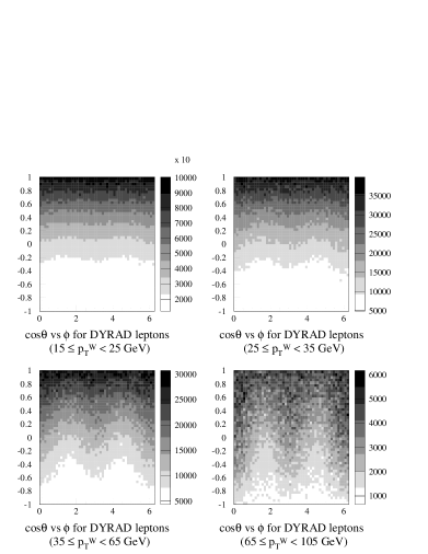
Figure 4: The $\cos\theta$ vs. $\phi$ phase space for the four $p_{T}^{W}$ bins, for the DYRAD generator simulation (arbitrary units).

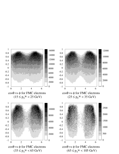
Figure 5: The $\cos\theta$ vs. $\phi$ phase space for the four $p_{T}^{W}$ bins, for the electron FMC signal simulation (arbitrary units).

Figure 6: The $\cos\theta$ vs. $\phi$ phase space for the four $p_{T}^{W}$ bins, for the muon FMC signal simulation (arbitrary units).

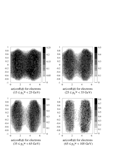
Figure 7: Acceptance times efficiency for the electrons as a function of $\cos\theta$ and $\phi$ in the Collins-Soper frame.

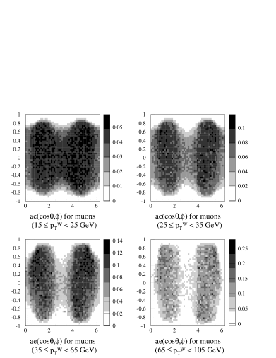
Figure 8: Acceptance times efficiency for the muons as a function of $\cos\theta$ and $\phi$ in the Collins-Soper frame.

We are especially interested in the product of overall acceptance times efficiency ($ae$) as a function of ($\cos\theta$,$\phi$) associated with each of the four $p_{T}^{W}$ bins We create 2-dimensional histograms of $\cos\theta$ vs. $\phi$ for each of the four $p_{T}^{W}$ bins, using the DYRAD simulation. This procedure is repeated after the events pass the FMC simulation, where the appropriate mixture of Run Ia and Run Ib $W$ leptons is used, based on FMC event yield predictions for all subdetectors.

The resulting plots are shown in Figures 4, 5, and 6, for DYRAD, FMC-electrons, and FMC-muons respectively. We subsequently divide the FMC 2-dimensional histograms by the corresponding DYRAD ones, producing the 2-dimensional differential acceptance times efficiency $ae(\cos\theta,\phi)$ of Figures 7 and 8, for electrons and muons respectively. The overall acceptance times efficiency is higher for the electrons. These $ae(\cos\theta,\phi)$ values are used for the $\cos\theta$-integration of the cross section, as described in Section VII.

V Background estimation

The main sources of background in the ($W\rightarrow e\nu_{e}$)+jet and ($W\rightarrow\mu\nu_{\mu}$)+jet processes are $Z$+jets events where the $Z$ is misidentified as a $W$ (“one-legged” $Z$), ($W\rightarrow\tau\nu_{\tau}$)+jet events, and QCD background resulting from jet misidentification. The $W+\gamma$ background is only a few events with run and event numbers the same as the $W+\gamma$ events of Christofek (2001); it is treated as a systematic uncertainty, which also gives an indication of the radiative effects in the measurement. This uncertainty is very small (see Section IX).

A small background contribution arises from $t\bar{t}$ production, where one of the produced $W$ bosons decays leptonically and the other $W$ boson decays hadronically to jets. This background is estimated to be $30\pm 7$ events for the electron sample Dittmann (1998) and $16\pm 3$ events for the muon sample, a 0.3% effect. An equally small background is the $Z\rightarrow\tau^{+}\tau^{-}$ production, where one of the tau leptons decays hadronically and the other one leptonically. This background is estimated to be $47\pm 1$ events in the electron sample Dittmann (1998), and $25\pm 1$ events in the muon sample, a 0.5% effect. To demonstrate the insignificance of the $t\bar{t}$ and $Z\rightarrow\tau^{+}\tau^{-}$ backgrounds, we perform our analysis including the charged lepton $\phi$ distribution for these background events, in several possible shapes, for the four $p_{T}^{W}$ bins. The resulting change in the extracted values of the angular coefficients is negligible compared to our systematic and statistical uncertainties. Thus, we ignore the backgrounds associated with $t\bar{t}$ production and $Z\rightarrow\tau^{+}\tau^{-}$ decays.

Finally, the cosmic ray background in the muon $W$+jet datasets is estimated to be significantly less than 0.1%, and is therefore neglected.

V.1 One-legged $Z$ background

To study this background we generate a DYRAD sample of $Z$+jet events and pass it through the FMC Monte Carlo simulation and the subsequent analysis program. This predicts how many $Z$ bosons are misidentified as $W$ bosons. In these cases, the $Z$ bosons satisfy all kinematic and lepton identification cuts for $W$ bosons, but one of their decay leptons, or legs, is undetected. The DYRAD cross section for $Z$+jet up to order $\alpha_{s}^{2}$ is 68.21 $\pm$ 0.37 pb. For this DYRAD simulation we used $Q^{2}=(M_{Z}^{\rm pole})^{2}=91.2$ GeV, the CTEQ4M($\Lambda=0.3$ GeV) parton distribution functions, 0.7-cone jets, jet-jet angular separation greater than 0.7 in $\eta_{\rm lab}$-$\phi_{\rm lab}$ space, and $E_{T}^{j}>10$ GeV. At the FMC level, we impose our usual $W$ boson event selection cuts and additionally require at least one “good” jet ($E_{T}^{\rm jet}>15$ GeV and $|\eta_{\rm lab}^{\rm jet}|<2.4$) that also passes the $\Delta R_{l-j}^{\rm lab}>0.7$ cut. These results are summarized in Table 3. Overall we expect $123\pm 5$ electron one-legged-Z+jet events and $337\pm 18$ muon one-legged-Z+jet events passing the $W$+jet cuts, without applying any cut on the W transverse momentum. Comparing these numbers to the FMC event yields for $W$+jet, the one-legged-Z+jet background is $(1.14\pm 0.06)\%$ for the electron $W$+jet and $(5.90\pm 0.43)\%$ for the muon $W$+jet sample. This background is higher for the muon sample, because of the limited coverage of the muon chambers, which is responsible for higher yields of one-legged muon $Z$ bosons.

To examine how this background affects the $W$+jet lepton $\phi$ distribution, we plot the $\phi$ distribution for the leptons from these processes for the four $p_{T}^{W}$ bins (Figures 9 and 10). We see that the same pattern of two maxima at $\frac{\pi}{2}$ and $\frac{3\pi}{2}$ is present. The background plots are normalized to the expected event yields from the FMC, multiplied by a factor of five (to make them visible), and superimposed on the signal FMC distributions, normalized to the signal FMC event yields. We include the one-legged $Z$ FMC $\phi$ distribution in the complete theoretical prediction of the $\phi$ distributions, in order to correctly extract the angular coefficients.

Figure 9: Electron $\phi$ distributions for the four $p_{T}^{W}$ bins for electron $W$+jet FMC events (solid histogram) and for $Z$+jet FMC background (multiplied by 5), where one of the electrons from the $Z$ decay is undetected and the other one passes the detection and analysis requirements (dashed histogram). The histograms are normalized to the electron FMC signal event yields.

Figure 10: Muon $\phi$ distributions for the four $p_{T}^{W}$ bins for muon $W$+jet FMC events (solid histogram) and for $Z$+jet FMC background (multiplied by 5), where one of the muons from the $Z$ decay is undetected and the other one passes the detection and analysis requirements (dashed histogram). The histograms are normalized to the muon FMC signal event yields.

Table 3: Monte Carlo background estimation of the number of electron and muon one-legged $Z$+jet events. The background fractions are calculated with respect to the FMC $W$+jet event yields.

One-legged $Z$+jet background
$p_{T}^{W}$ (GeV)	$N_{e}$	Fraction	$N_{\mu}$	Fraction
15–25	47 $\pm$ 2	1.22 $\pm$ 0.07 %	127 $\pm$ 7	6.26 $\pm$ 0.47 %
25–35	30 $\pm$ 1	1.14 $\pm$ 0.05 %	82 $\pm$ 4	5.92 $\pm$ 0.40 %
35–65	25 $\pm$ 1	1.01 $\pm$ 0.05 %	72 $\pm$ 4	5.48 $\pm$ 0.41 %
65–105	5 $\pm$ 0	0.96 $\pm$ 0.03 %	12 $\pm$ 1	4.30 $\pm$ 0.42 %

V.2 ($W\rightarrow\tau\nu$)+jet background

If the $W$ boson decays to a $\tau$ that subsequently decays leptonically, the three final neutrinos contribute to the $E_{T}\!\!\!\!\!\!\!/\,\,\,\,\,\,$, which is incorrectly associated with a single neutrino. The signal of one charged lepton along with the $E_{T}\!\!\!\!\!\!\!/\,\,\,\,\,\,$ mimics that of a $W$ directly decaying to the charged lepton. Most of the tau background is removed when we utilize the fact that the charged lepton and $E_{T}\!\!\!\!\!\!\!/\,\,\,\,\,\,$ coming from the $\tau$ decay are soft. As a result, the $W$ transverse mass in the $\tau$ events is significantly smaller than that in the electron or muon events. By applying the $p_{T}$ cuts for the leptons and the $W$ transverse mass cut, we remove $92\%$ of the tau $W$+jet events at the DYRAD generator level.

To study the remaining tau background we start with a tau $W$+jet DYRAD sample ($Q^{2}=(M_{W}^{\rm pole})^{2}$, CTEQ4M($\Lambda=0.3$ GeV) parton distribution function and 0.7-cone jets in $\eta_{\rm lab}$-$\phi_{\rm lab}$ space), and we let the tau decay to an electron or a muon. We then vector-sum the three neutrinos resulting from the $W$ and tau decays to form a single $E_{T}\!\!\!\!\!\!\!/\,\,\,\,\,\,$. Subsequently, we pass the events through the FMC detector simulator to see how many events pass the $W$+jet cuts after they are weighted by the detector acceptances and efficiencies. The branching ratios for the tau decays we use are 17.83 % for electrons and 17.37 % for muons Hagiwara et al. (2002). At the FMC level, we require at least one “good” jet ($E_{T}^{\rm jet}>15$ GeV and $|\eta_{\rm lab}^{\rm jet}|<2.4$) that also passes the $\Delta R_{l-j}^{\rm lab}>0.7$ cut. The tau background results are presented in Table 4. Overall we expect $247\pm 9$ tau electrons and $130\pm 7$ tau muons to infiltrate the $W$+jet samples, without applying any cut on the W transverse momentum. Comparing these numbers to the FMC event yields for the electron and muon $W$+jet samples, the tau background is $(2.28\pm 0.12)\%$ for the electron $W$+jet sample, and $(2.28\pm 0.17)\%$ for the muon $W$+jet sample.

To see how this background affects the $W$+jet lepton $\phi$ distribution, we plot the $\phi$ distribution for the leptons resulting from leptonic tau decays in $W$+jets events for the four $p_{T}^{W}$ bins (Figures 11 and 12). We see that the pattern of two maxima at $\frac{\pi}{2}$ and $\frac{3\pi}{2}$ is again present. The background plots are normalized to the expected event yields from the FMC, multiplied by a factor of five, and superimposed on the signal FMC distributions, normalized to the signal FMC event yields. We include the $\tau$-background FMC $\phi$ distribution in the complete theoretical prediction of the $\phi$ distributions, in order to correctly extract the angular coefficients.

Figure 11: Electron $\phi$ distributions for the four $p_{T}^{W}$ bins for electron $W$+jet FMC events (solid histogram) and for tau $W$+jet FMC background (multiplied by 5), where the tau decays to an electron (dashed histogram). The histograms are normalized to the FMC signal event yields.

Figure 12: Muon $\phi$ distributions for the four $p_{T}^{W}$ bins for muon $W$+jet FMC events (solid histogram) and for tau $W$+jet FMC background (multiplied by 5), where the tau decays to a muon (dashed histogram). The histograms are normalized to the FMC signal event yields.

Table 4: Monte Carlo background estimation of the number of electron and muon $W$+jet events, where the $W$ decays to a tau and the electron or muon is the decay product of the tau. The fractions of the backgrounds are calculated with respect to the FMC $W$+jet event yields.

($W\rightarrow\tau\;\bar{\nu}_{\tau}\rightarrow\bar{\nu}_{\tau}\;\nu_{\tau}\;\bar{\nu}_{e/\mu}\;e/\mu$)+jet background
$p_{T}^{W}$ (GeV)	$N_{e}$	Fraction	$N_{\mu}$	Fraction
15–25	86 $\pm$ 3	2.22 $\pm$ 0.11 %	45 $\pm$ 2	2.22 $\pm$ 0.15 %
25–35	57 $\pm$ 2	2.16 $\pm$ 0.10 %	30 $\pm$ 2	2.17 $\pm$ 0.18 %
35–65	56 $\pm$ 2	2.26 $\pm$ 0.11 %	30 $\pm$ 2	2.28 $\pm$ 0.19 %
65–105	15 $\pm$ 1	2.89 $\pm$ 0.22 %	8 $\pm$ 0	2.87 $\pm$ 0.14 %

V.3 QCD background

The QCD background in the case of inclusive $W$ production and decay consists predominantly of dijet events, where one of the jets is misidentified as a lepton and the other one is not detected, resulting in the creation of $E_{T}\!\!\!\!\!\!\!/\,\,\,\,\,\,$. In the $W$+jet case, the QCD background is multijet events, where one of the jets is detected, one is lost or mismeasured (resulting in $E_{T}\!\!\!\!\!\!\!/\,\,\,\,\,\,$) and one is misidentified as a charged lepton to erroneously reconstruct a $W$. The number and distribution of QCD background events in the four $p_{T}^{W}$ bins are determined from the Run Ia and Run Ib CDF data.

To measure the expected number of QCD background events in our data samples we look at leptons with isolation (ISO), defined in Section II, greater than 0.2. Our signal is in the ISO $<$ 0.1 region and most of the events with lepton ISO $>$ 0.2, but not all of them, are QCD background events. The upper histogram of Figure 13 shows the isolation distribution of the electrons from $W$+jet events, for the first $p_{T}^{W}$ bin. When plotted on a semi-log scale, the ISO $<$ 0.1 and the ISO $>$ 0.2 regions can be approximated with two straight lines. The technique we use extrapolates the ISO $>$ 0.2 line into the ISO $<$ 0.1 signal region to calculate its integral and obtain the number of events in the signal region, using the assumption that the QCD background shape is not altered in that region. This method would give us the true number of QCD background events, if the ISO $>$ 0.2 region was filled exclusively with QCD events. In reality, only a fraction of these events are true QCD background, the rest being $W$+jet events. Since we expect to have some $W$+jet events in the region of lepton isolation from 0.1 to 0.2, we fit the area above 0.2 with a straight line (in the semi-log histogram), which describes the QCD background. We also fit five continuous regions of lepton isolation, around the central region of ISO=0.20 to ISO=0.65 (namely 0.15-0.65, 0.25-0.65, 0.15-0.60, 0.20-0.65, and 0.25-0.70) to obtain a systematic uncertainty for this procedure.

Figure 13: Isolation of the electron in $W$+jet events (upper histogram) and the difference in the azimuthal angles of the electron and the jet for high isolation events (lower histogram). These histograms are used to estimate the QCD background in the electron $W$+jet data, for the $15\leq p_{T}^{W}\leq 25$ GeV bin (see text). Corresponding histograms are used for the estimation of the QCD background in the three other electron $W$+jet $p_{T}^{W}$ bins.

Table 5: The linear least-squares fit parameterization of the $\Delta\phi_{l-j}^{\rm lab}$ distribution for ISO $>0.2$ electron $W$+jet events (second column) allows us to estimate the number of ISO $>0.2$ $W$+jet events in the $\Delta\phi_{l-j}^{\rm lab}>2.5$ region. The integral of this line, divided by the bin width ($\pi$/30) of the $\Delta\phi_{l-j}^{\rm lab}$ histogram, is the number of $W$+jet events with ISO $>0.2$ and $\Delta\phi_{l-j}^{\rm lab}>2.5$ shown in the third column. These events are subtracted from the total number of ($W$+jet + QCD) background events in the ISO $>0.2$ and $\Delta\phi_{l-j}^{\rm lab}>2.5$ region (fourth column). The result is divided by the total number of events in the ISO $>0.2$ region, to obtain an estimate of the fraction of true QCD background events (fifth column).

	Fit parameterization of electron	Electron $W$+jet events with	($W$+jet)+QCD events with	Fraction of
$p_{T}^{W}$ (GeV)	$W$+jet events with ISO $>0.2$	ISO $>0.2$ and $\Delta\phi_{l-j}^{\rm lab}>2.5$	ISO $>0.2$ and $\Delta\phi_{l-j}^{\rm lab}>2.5$	true QCD events
15–25	$2.21\times\Delta\phi_{l-j}^{\rm lab}-0.05$	37.9	257	0.66=(257-37.9)/332
25–35	$0.70\times\Delta\phi_{l-j}^{\rm lab}+0.78$	16.9	98	0.58=(98-16.9)/141
35–65	$1.04\times\Delta\phi_{l-j}^{\rm lab}+0.45$	20.6	49	0.31=(49-20.6)/91
65–105	$0.17\times\Delta\phi_{l-j}^{\rm lab}+0.73$	7.5	10	0.13=(10-7.5)/20

Table 6: The number of electron W+jet events, the number of QCD background events before correction and their percentage in the signal region, and the fraction of true QCD background events and their percentage in the signal region, for the four $p_{T}^{W}$ bins (see text for details).

	Number of	QCD events	Percentage of QCD	Fraction of	Percentage of
$p_{T}^{W}$ (GeV)	electron $W$+jet	before correction	before correction	true QCD events	QCD background
15–25	5166	423${}^{+77}_{-42}$	8.18${}^{+1.11}_{-0.81}\%$	0.66${}^{+0.04}_{-0.04}$	5.40${}^{+0.80}_{-0.63}\%$
25–35	3601	353${}^{+26}_{-148}$	9.80${}^{+0.74}_{-4.1}\%$	0.58${}^{+0.07}_{-0.08}$	5.68${}^{+0.81}_{-2.50}\%$
35–65	3285	54${}^{+151}_{-25}$	1.64${}^{+4.60}_{-0.75}\%$	0.31${}^{+0.13}_{-0.13}$	0.51${}^{+1.44}_{-0.32}\%$
65–105	624	14${}^{+8}_{-3}$	2.24${}^{+1.24}_{-0.27}\%$	0.13${}^{+0.87}_{-0.13}$	0.29${}^{+1.96}_{-0.29}\%$

Since not all of the extrapolated region is QCD background, we obtain a measurement of the percentage of the true QCD background in the electron $W$+jet sample above electron isolation of 0.1, by making a histogram of $\Delta\phi_{l-j}^{\rm lab}$ for the events with ISO $>$ 0.2, where $\Delta\phi_{l-j}^{\rm lab}$ is the difference in the $\phi$ angle between the electron and the highest-$E_{T}$ jet, with no other requirements for that jet. We expect the $\Delta\phi_{l-j}^{\rm lab}$ distribution to be almost flat for the $W$+jet events, because no correlation exists between the jet and the lepton $\phi$ directions. In reality, this distribution decreases at low $\Delta\phi_{l-j}^{\rm lab}$, due to the application of the lepton isolation cut in our data. For QCD background, we expect the $\Delta\phi_{l-j}^{\rm lab}$ between the highest $E_{T}$ jet and the jet resembling the lepton to peak at $\pi$.

Figure 14: Isolation of the muon in $W$+jet events (upper histogram) and the difference in the azimuthal angles of the muon and the jet for high isolation events (lower histogram). These histograms are used to estimate the QCD background in the muon $W$+jet data, for the $15\leq p_{T}^{W}\leq 25$ GeV bin (see text). Corresponding histograms are used for the estimation of the QCD background in the three other muon $W$+jet $p_{T}^{W}$ bins. At low $\Delta\phi_{l-j}^{\rm lab}$ the distribution increases, due to bremsstrahlung processes associated with residual muon $Z$+jet background in the muon $W$+jet sample. These events disappear if we apply the ${\tt zmuo\_veto}$ cut. (see text).

The lower histogram of Figure 13 shows the $\Delta\phi_{l-j}^{\rm lab}$ for the events with lepton isolation greater than 0.2 for electron $W$+jet events and for the first $p_{T}^{W}$ bin. We fit the region $\Delta\phi_{l-j}^{\rm lab}\leq 2.5$ ($W$+jet contribution) with a straight line. The region of the histogram $\Delta\phi_{l-j}^{\rm lab}>2.5$ above that line corresponds to true QCD background. By dividing this part of the histogram by the total number of events with ISO $>$ 0.2, we determine the true fraction of QCD background in the ISO $>$ 0.2 region. We expect the same fraction to be valid in the signal region (ISO $<0.1$). Therefore, the number of true QCD background events is obtained by multiplying the number of ISO $<$ 0.1 events (as obtained by extrapolating the ISO $>$ 0.2 line into the signal region of the lepton isolation plot) by the QCD background fraction obtained from the $\Delta\phi_{l-j}^{\rm lab}$ plot. The procedure is repeated for the four $p_{T}^{W}$ bins. Table 5 shows the extracted fraction of QCD background in the ISO $>$ 0.2 region for the four $p_{T}^{W}$ bins. The electron $W$+jet QCD background results are presented in Table 6.

In the study of the QCD background in the muon sample we face a new problem. We originally apply a cut to muon $W$+jet data (${\tt zmuo\_veto}$) in order to remove events that are consistent with the production of a $Z$ boson, where one of the muons is non-isolated because it fails one (and only one) of the following cuts:

• The muon isolation cut ISO $<0.1$

• The electromagnetic calorimeter cut $E^{\rm EM}<2$ GeV

• The hadron calorimeter cut $E^{\rm HAD}<6$ GeV

These dimuon events are true $Z$ bosons that look like $W$ bosons because one muon does not pass one of the above cuts due to inner bremsstrahlung or bremmsstrahlung in the electromagnetic or hadronic calorimeters. The ${\tt zmuo\_veto}$ cut mainly affects the tail of the muon isolation distribution (ISO $>0.2$) and causes us to underestimate the QCD background, since we use that tail to estimate it. Therefore, for the muon $W$+jet samples, for the purposes of determination of QCD background, we neglect this cut, in order to remove this bias at high muon isolation (ISO $>$ 0.2) and make the transition from the low to high isolation smooth. Some of the muon $Z$ background is thus counted as QCD background; however we do not expect it to radically affect our QCD background estimation. In the isolation method we fit the background starting from ISO=0.17 to ISO=0.40, to increase the statistical significance of our estimation. We also fit five continuous regions of lepton isolation, around the central region of ISO=0.17 to ISO=0.40 (namely 0.16-0.40, 0.18-0.40, 0.16-0.35, 0.17-0.40, and 0.18-0.45) to obtain a systematic uncertainty for this procedure. The upper histogram of Figure 14 shows the isolation distribution and fits for the muon $W$+jet events and for the first $p_{T}^{W}$ bin.

We obtain a measurement of the percentage of the true QCD background in the muon $W$+jet sample above muon isolation of 0.2, by making a histogram of $\Delta\phi_{l-j}^{\rm lab}$ for the events with ISO $>$ 0.2, where $\Delta\phi_{l-j}^{\rm lab}$ is the difference in the $\phi$ angle between the muon and the highest-$E_{T}$ jet, with no other requirements for that jet. The lower histogram of Figure 14 shows $\Delta\phi_{l-j}^{\rm lab}$ for the events with isolation greater than 0.2 for muon $W$+jet events, for the first $p_{T}^{W}$ bin. The peak in the $\Delta\phi_{l-j}^{\rm lab}=0$ region is due to the muon bremsstrahlung processes that are not suppressed after we relax the ${\tt zmuo\_veto}$ cut. We ignore these events when we fit to the straight line describing the $W$+jet events with high isolation muons.

Table 7: The linear least-squares fit parameterization of the $\Delta\phi_{l-j}^{\rm lab}$ distribution for ISO $>0.2$ muon $W$+jet events (second column) allows us to estimate the number of ISO $>0.2$ $W$+jet events in the $\Delta\phi_{l-j}^{\rm lab}>2.5$ region. The integral of this line, divided by the bin width ($\pi$/30) of the $\Delta\phi_{l-j}^{\rm lab}$ histogram, is the number of $W$+jet events with ISO $>0.2$ and $\Delta\phi_{l-j}^{\rm lab}>2.5$ shown in the third column. These events are subtracted from the total number of ($W$+jet + QCD) background events in the ISO $>0.2$ and $\Delta\phi_{l-j}^{\rm lab}>2.5$ region (fourth column). The result is divided by the total number of events in the ISO $>0.2$ region, to obtain an estimate of the fraction of true QCD background events (fifth column).

	Fit parameterization of muon	Muon $W$+jet events with	($W$+jet)+QCD events with	Fraction of
$p_{T}^{W}$ (GeV)	$W$+jet events with ISO $>0.2$	ISO $>0.2$ and $\Delta\phi_{l-j}^{\rm lab}>2.5$	ISO $>0.2$ and $\Delta\phi_{l-j}^{\rm lab}>2.5$	true QCD events
15–25	$0.29\times\Delta\phi_{l-j}^{\rm lab}+1.31$	13	164	0.52=(164-13)/288
25–35	$0.46\times\Delta\phi_{l-j}^{\rm lab}+0.79$	12.8	69	0.40=(69-12.8)/140
35–65	$0.25\times\Delta\phi_{l-j}^{\rm lab}+1.02$	10.5	19	0.14=(19-10.5)/61
65–105	$0\times\Delta\phi_{l-j}^{\rm lab}+1$	6.1	1	$0=0/6$

Table 8: The number of muon W+jet events without the application of the ${\tt zmuo\_veto}$ cut, the number of QCD background events before correction and their percentage in the signal region, and the fraction of true QCD background events and their percentage in the signal region, for the four $p_{T}^{W}$ bins (see text for details).

	Number of	QCD events	Percentage of QCD	Fraction of	Percentage of
$p_{T}^{W}$ (GeV)	muon $W$+jet	before correction	before correction	true QCD events	QCD background
15–25	2779	280${}^{+102}_{-25}$	10.07${}^{+3.68}_{-0.90}\%$	0.52${}^{+0.05}_{-0.04}$	5.24${}^{+1.98}_{-0.62}\%$
25–35	1943	103${}^{+129}_{-4}$	5.30${}^{+6.64}_{-0.21}\%$	0.40${}^{+0.08}_{-0.08}$	2.12${}^{+2.69}_{-0.43}\%$
35–65	2002	139${}^{+50}_{-21}$	6.94${}^{+2.50}_{-1.05}\%$	0.14${}^{+0.22}_{-0.14}$	0.97${}^{+1.57}_{-0.97}\%$
65–105	389	11${}^{+0}_{-0}$	2.70${}^{+0.00}_{-0.00}\%$	$0^{+1}_{-0}$	0${}^{+2.7}_{-0}\%$

Table 7 shows the extracted fraction of QCD background in the ISO $>$ 0.2 region for the four $p_{T}^{W}$ bins. The muon $W$+jet QCD background results are presented in Table 8. For the highest muon $p_{T}^{W}$ bin the predicted number of true $W$+jet events is greater than the total number of events with ISO $>$ 0.2 and $\Delta\phi_{l-j}^{\rm lab}>2.5$, which results in a fraction of true QCD background events above ISO $>$ 0.2 equal to zero.

After we calculate the percentage of the QCD background in the signal region, we multiply it by the CDF $W$+jet event yields to obtain the absolute prediction of the number of QCD background events in each of the four $p_{T}^{W}$ bins, for both and electron and muon $W$+jet data. The results are presented in Table 9.

Figure 15: The Collins-Soper $\phi$ distribution of electrons from $W$+jet events with ISO $>0.2$ and $\Delta\phi_{l-j}^{\rm lab}>2.5$ for each of the four $p_{T}^{W}$ bins. These events are predominantly QCD background events. We fit the distribution of the first three $p_{T}^{W}$ bins with two Gaussians on top of two straight lines. For the highest $p_{T}^{W}$ bin we use the distribution of the total QCD background, normalized to the number of the QCD events in this bin. (see text for details).

Figure 16: The Collins-Soper $\phi$ distribution of muons from $W$+jet events with ISO $>0.2$ and $\Delta\phi_{l-j}^{\rm lab}>2.5$ for each of the four $p_{T}^{W}$ bins. These events are predominantly QCD background events. We fit the distribution of the first two $p_{T}^{W}$ bins with two Gaussians on top of two straight lines. For the two highest $p_{T}^{W}$ bins we use the distribution of the total background, normalized to the number of the QCD events in those bins.

Table 9: QCD background estimation for the electron and muon $W$+jet events. The fractions of the backgrounds are calculated with respect to the CDF Data $W$+jet events.

QCD background
$p_{T}^{W}$ (GeV)	$N_{e}$	Fraction	$N_{\mu}$	Fraction
15–25	279 ${}^{+41}_{-33}$	5.40 ${}^{+0.80}_{-0.63}$ %	148 ${}^{+56}_{-17}$	5.24 ${}^{+1.98}_{-0.62}$ %
25–35	205 ${}^{+29}_{-90}$	5.68 ${}^{+0.81}_{-2.50}$ %	40 ${}^{+50}_{-8}$	2.12 ${}^{+2.69}_{-0.43}$ %
35–65	17 ${}^{+47}_{-11}$	0.51 ${}^{+1.44}_{-0.32}$ %	18 ${}^{+30}_{-18}$	0.97 ${}^{+1.57}_{-0.97}$ %
65–105	2 ${}^{+12}_{-2}$	0.29 ${}^{+1.96}_{-0.29}$ %	0 ${}^{+10}_{-0}$	0 ${}^{+2.7}_{-0}$%

Table 10: Summary of electron $W$+jet backgrounds. The background fractions are calculated with respect to the FMC signal event yields for the electroweak backgrounds and with respect to the data for the QCD background.

Electron $W$+jet Backgrounds
Background	$p_{T}^{W}$=15–25 GeV	$p_{T}^{W}$=25–35 GeV	$p_{T}^{W}$=35–65 GeV	$p_{T}^{W}$=65–105 GeV
$W\rightarrow\tau\nu_{\tau}$	86 $\pm$ 3 (2.22 %)	57 $\pm$ 2 (2.16 %)	56 $\pm$ 2 (2.26 %)	15 $\pm$ 1 (2.89%)
$Z\rightarrow e^{+}e^{-}$	47 $\pm$ 2 (1.22 %)	30 $\pm$ 1 (1.14 %)	25 $\pm$ 1 (1.01 %)	5 $\pm$ 0 (0.96 %)
QCD	$279^{+41}_{-33}$ (5.40 %)	$205^{+29}_{-90}$ (5.68 %)	$17^{+47}_{-11}$ (0.51 %)	$2^{+12}_{-2}$ (0.29 %)

Table 11: Summary of muon $W$+jet backgrounds. The background fractions are calculated with respect to the FMC signal event yields for the electroweak backgrounds and with respect to the data for the QCD background.

Muon $W$+jet Backgrounds
Background	$p_{T}^{W}$=15–25 GeV	$p_{T}^{W}$=25–35 GeV	$p_{T}^{W}$=35–65 GeV	$p_{T}^{W}$=65–105 GeV
$W\rightarrow\tau\nu_{\tau}$	45 $\pm$ 2 (2.22 %)	30 $\pm$ 2 (2.17 %)	30 $\pm$ 2 (2.28 %)	8 $\pm$ 0 (2.87%)
$Z\rightarrow\mu^{+}\mu^{-}$	127 $\pm$ 7 (6.26 %)	82 $\pm$ 4 (5.92 %)	72 $\pm$ 4 (5.48 %)	12 $\pm$ 1 (4.30 %)
QCD	$148^{+56}_{-17}$ (5.24 %)	$40^{+50}_{-8}$ (2.12 %)	$18^{+30}_{-18}$ (0.97 %)	$0^{+10}_{-0}$ (0 %)

Table 12: The expected total event yields for inclusive $W$+jet production. The signal and electroweak backgrounds are calculated up to order $\alpha_{s}^{2}$. The PDF and $Q^{2}$ systematics have also been included (second set of uncertainties).

Expected signal+background event yields for inclusive $W$+jet production
	Electrons			Muons
$p_{T}^{W}$ (GeV)	$N_{e}({\rm Signal})$	$N_{e}({\rm Background})$	$N_{e}$(Total prediction)	$N_{\mu}({\rm Signal})$	$N_{\mu}({\rm Background})$	$N_{\mu}$(Total prediction)
15–25	3867 $\pm$ 137	$412^{+41}_{-33}$	$4279^{+148}_{-146}$$+880$/$-660$	2027 $\pm$ 102	$320^{+57}_{-19}$	$2347^{+124}_{-112}$$+484$/$-330$
25–35	2632 $\pm$ 93	$292^{+29}_{-90}$	$2924^{+100}_{-132}$$+598$/$-408$	1384 $\pm$ 66	$152^{+50}_{-10}$	$1536^{+88}_{-72}$$+329$/$-224$
35–65	2474 $\pm$ 87	$98^{+47}_{-11}$	$2572^{+102}_{-91}$$+562$/$-383$	1314 $\pm$ 67	$120^{+31}_{-19}$	$1434^{+79}_{-75}$$+312$/$-213$
65–105	518 $\pm$ 18	$22^{+12}_{-2}$	$540^{+22}_{-19}$$+118$/$-81$	279 $\pm$ 14	$20^{+10}_{-1}$	$299^{+18}_{-15}$$+66$/$-45$

To complete the study of the QCD background we need to estimate its shape to properly include this background in the Standard Model prediction of the lepton $\phi$ distribution in the CS frame, for each of the four $p_{T}^{W}$ bins. We plot $\phi$ for the events with ISO $>$ 0.2 and $\Delta\phi_{l-j}^{\rm lab}>2.5$ for the electrons and muon datasets, as shown in Figures 15 and 16, respectively. We fit the distributions to the sum of two Gaussians and two straight lines. For the last $p_{T}^{W}$ bin of the electrons and the last two $p_{T}^{W}$ bins of the muons, there are not enough statistics for the fit, so we use the total distributions (for $15\leq p_{T}^{W}\leq 105$ GeV) normalized to the number of events for those high $p_{T}^{W}$ bins. We do not expect the shape of the QCD background to be significantly altered with increasing $p_{T}^{W}$. We assume that these distributions are the same as the ones in the signal region (ISO $<0.1$) after they are properly normalized. We use these distributions to add the QCD background to the Standard Model prediction, after they are normalized to the expected number of QCD background events, given by Table 9.

V.4 Summary of backgrounds and Standard Model event yields prediction.

Backgrounds for electron and muon $W$+jet events for each of the four $p_{T}^{W}$ bins are summarized in Tables 10 and 11 respectively. We obtain the total $W$+jet event yield prediction by adding these backgrounds to the FMC $W$+jet signal prediction of Table 2. To obtain the final uncertainties, we add linearly the uncertainties associated with the $W$+jet signal and electroweak background and add the result to the QCD background uncertainty in quadrature. The total $W$+jet event yields after the inclusion of the backgrounds are presented in Table 12. The PDF and $Q^{2}$ systematic uncertainties are also included (see Section IX).

Figure 17: The transverse momentum of the $W$ for the electron $W$+jet data sample (points) along with the FMC signal simulation including backgrounds (solid histogram). The backgrounds are multiplied by 5, to be visible. The data and expected signal+background distributions are normalized to unity.

Figure 18: The transverse mass of the $W$ for the electron $W$+jet data sample (points) along with the FMC signal simulation including backgrounds (solid histogram). The backgrounds are multiplied by 5, to be visible. The data and expected signal+background distributions are normalized to unity.

Figure 19: The transverse momentum of the $W$ for the muon $W$+jet data sample (points) along with the FMC signal simulation including backgrounds (solid histogram). The backgrounds are multiplied by 5, to be visible. The data and expected signal+background distributions are normalized to unity.

Figure 20: The transverse mass of the $W$ for the electron $W$+jet data sample (points) along with the FMC signal simulation including backgrounds (histogram), for the four $p_{T}^{W}$ bins. The data and expected signal+background distributions are normalized to unity.

Figure 21: The transverse mass of the $W$ for the muon $W$+jet data sample (points) along with the FMC signal simulation including backgrounds (solid histogram). The backgrounds are multiplied by 5, to be visible. The data and expected signal+background distributions are normalized to unity.

Figure 22: The transverse mass of the $W$ for the muon $W$+jet data sample (points) along with the FMC signal simulation including backgrounds (histogram), for the four $p_{T}^{W}$ bins. The data and expected signal+background distributions are normalized to unity.

VI Comparison Between Expected and Observed $W$ Distributions

We study the expected (FMC) $W$ kinematical distributions after the inclusion of backgrounds and compare them to the experimental distributions. Figures 17 and 19 show the $W$ transverse momentum for electrons and muons respectively. The observed and simulated distributions have been normalized to unity. We observe good agreement between the observed and simulated $p_{T}^{W}$ distributions. Figure 18 shows the $W$ transverse mass distribution for the electron $W$+jet dataset and for the DYRAD events passed through the FMC detector simulation. Figure 20 shows the same distributions for the four $p_{T}^{W}$ bins. Figures 21 and 22 show the same distributions for the muon $W$+jet datasets. The observed and simulated distributions are again normalized to unity. In all of the above plots, the FMC distributions are produced with properly weighted signal and background contributions, for electron and muon detector regions.

VII Direct measurement of the azimuthal angle of the charged leptons from $W$ decays in the Collins-Soper frame

For each $W$ event we boost to the $W$ rest-frame to calculate the azimuthal angle of the charged lepton. The longitudinal momentum of the $W$ ($p_{Z}^{W}$) is not known, because the longitudinal momentum of the neutrino is not measurable, so we use the mass of the $W$ to constrain it. For a particular event, the longitudinal momentum of the neutrino is constrained by the mass of the $W$, according to the equation:

$$p_{z}^{\nu}=\frac{1}{(2p_{T}^{l})^{2}}\left(Ap_{z}^{l}\pm E^{l}\sqrt{A^{2}-4(p_{T}^{l})^{2}(p_{T}^{\nu})^{2}}\right),$$ (2)

where

$$A=M_{W}^{2}+(p_{T}^{W})^{2}-(p_{T}^{l})^{2}-(p_{T}^{\nu})^{2},$$ (3)

$E^{l}$ is the energy of the charged lepton, $p_{T}^{l}$ is its transverse momentum, $p_{z}^{l}$ is its longitudinal momentum, $p_{T}^{\nu}$ is the neutrino transverse momentum, and $p_{T}^{W}$ is the transverse momentum of the $W$. This equation is unique for every event, since the kinematics of the lepton and neutrino, as well as the mass of the $W$, contribute to the shape of the curve $p_{z}^{\nu}=f(M_{W})$. If the mass of the $W$ was known on an event by event basis, there would be a two-fold ambiguity in the value of ${p}_{z}^{\nu}$ of the neutrino in the laboratory frame. Because the $W$ boson has a finite width given by a PDF-convoluted Breit-Wigner distribution, $BW(M)$, we actually have two distributions of possible values of $p_{z}^{\nu}$, $BW(M(p_{z}^{\nu}))$, where $M(p_{z}^{\nu})$ is the mass of the $W$ as a function of the neutrino longitudinal momentum for the particular kinematics of the event.

The choice of one of the two neutrino longitudinal momentum solutions does not affect the $\phi$ analysis, since both solutions result in the same charged lepton $\phi$ in the CS frame. For this analysis, only the choice of the $W$ mass is of interest. The choice is made based on the 2-dimensional $M^{W}$ vs. $M_{T}^{W}$ histograms constructed with DYRAD events. For a specific $M_{T}^{W}$ we use a probability distribution of $W$ masses and randomly select one for each event, based on that distribution. This method was devised to better reconstruct the $|\cos(\theta)|$ distribution Strologas (2002), since the polar angle is very sensitive to the selection of the $W$ mass. In our analysis, the azimuthal angle is not affected by the choice of mass, so the answer is almost the same even if we choose a mass based on the Breit-Wigner distribution and the requirement that the mass is greater than the measured transverse mass.

After obtaining a $\phi$ for every event, we proceed to analyze our sample. Theoretically, the $W$ differential cross section, integrated over $\cos\theta$ and $y$ is given by:

$$\frac{d\sigma}{d(p_{T}^{W})^{2}d\phi}=C(1+\beta_{1}\cos{\phi}+\beta_{2}\cos{2\phi}$$

$$+\beta_{3}\sin{\phi}+\beta_{4}\sin{2\phi}),$$ (4)

where

$$C=\frac{1}{2\pi}\frac{d\sigma}{d(p_{T}^{W})^{2}},\>\beta_{1}=\frac{3\pi}{16}A_{3}(p_{T}^{W}),\>\beta_{2}=\frac{A_{2}(p_{T}^{W})}{4},$$

$$\beta_{3}=\frac{3\pi}{16}A_{7}(p_{T}^{W}),\>\beta_{4}=\frac{A_{5}(p_{T}^{W})}{2}.$$ (5)

The theoretical $\phi$ distributions for the charged lepton from $W$ boson decay in $W$+jet production are shown in Figure 2.

From Equations (4) and (5), the reader might conclude that only the $A_{2}$, $A_{3}$, $A_{5}$, and $A_{7}$ coefficients are measurable with the $\phi$ analysis, since the other angular coefficients are integrated out. However, in the actual $W$+jet data samples, what we measure is the number of events:

$$N(p_{T}^{W},\phi)=$$ (6)

$$\int\frac{d\sigma}{d(p_{T}^{W})^{2}d\phi d\cos\theta}ae(p_{T}^{W},\cos\theta,\phi)d\cos\theta\int{\cal L}dt$$

$$+ N_{bg}(p_{T}^{W},\phi),$$

where ${\cal L}$ is the instantaneous luminosity and $ae(p_{T}^{W},\cos\theta,\phi)$ is the overall acceptance times efficiency, determined in Section IV, for a particular $W$ transverse momentum and region in the $(\cos\theta,\phi)$ phase space. The quantity $N_{bg}(p_{T}^{W},\phi)$ is the background for the given $\phi$ bin and $p_{T}^{W}$, estimated in Section V. Combining Equations (6) and (1), the measured distribution is

$$N(p_{T}^{W},\phi) = C^{\prime}(f_{-1}(p_{T}^{W},\phi)+\sum_{i=0}^{7}A_{i}(p_{T}^{W})f_{i}(p_{T}^{W},\phi))$$ (7)

$$+ N_{bg}(p_{T}^{W},\phi),$$

where $C^{\prime}=C\int{\cal L}dt$. The $f_{i}$ are fitting functions, which are integrals of the product of the explicit functions $g_{i}(\cos\theta,\phi)$ and $ae(\cos\theta,\phi)$:

$$f_{i}(p_{T}^{W},\phi)=\int_{0}^{\pi}g_{i}(\theta,\phi)ae(p_{T}^{W},\cos\theta,\phi)d\cos\theta,$$ (8)

$$i=-1,\ldots,7$$

where

$$g_{-1}(\theta,\phi) = 1+\cos^{2}{\theta}$$

$$g_{0}(\theta,\phi) = \frac{1}{2}(1-3\cos^{2}{\theta})$$

$$g_{1}(\theta,\phi) = \sin{2\theta}\cos{\phi}$$

$$g_{2}(\theta,\phi) = \frac{1}{2}\sin^{2}{\theta}\cos{2\phi}$$

$$g_{3}(\theta,\phi) = \sin{\theta}\cos{\phi}$$

$$g_{4}(\theta,\phi) = \cos{\theta}$$

$$g_{5}(\theta,\phi) = \sin^{2}{\theta}\sin{2\phi}$$

$$g_{6}(\theta,\phi) = \sin{2\theta}\sin{\phi}$$

$$g_{7}(\theta,\phi) = \sin{\theta}\sin{\phi}$$

Because we multiply the $g_{i}(\theta,\phi)$ functions by $ae(p_{T}^{W},\cos\theta,\phi)$ before integrating over $\cos\theta$, no $f_{i}$ is exactly zero and all of the angular coefficients $A_{i}$ are in principle measurable. We have verified that the FMC-simulated $\phi$ distributions, fitted with a linear combination of $f_{i}$, result in angular coefficient values consistent with the SM predictions Strologas and Errede (2005). This result supports the self-consistency of the method.

We use Simpson integration for the calculation of the $f_{i}$ fitting functions given by Equation (8). The explicit functions $g_{i}(\theta,\phi)$ are integrated over $\cos\theta$, after they are weighted with the value of $ae(p_{T}^{W},\cos\theta,\phi)$ extracted from the 2-dimensional histograms of Figures 7 and 8.

Although the use of Equation (7) allows us in principle to measure all of the angular coefficients, in reality, the current statistics do not allow us to make a significant measurement of angular coefficients other than $A_{2}$ and $A_{3}$. This is due to the fact that the fitting functions $f_{i\neq 2,3}$ are small, and the $\phi$ distributions are insensitive to large variations of the corresponding angular coefficients. Figure 23 shows how the expected electron $\phi$ distributions are modified as the angular coefficients $A_{i}$ are varied, one coefficient at a time (the muon $\phi$ distributions are almost identical). Using Equation (7), we vary $A_{0}$, $A_{2}$, and $A_{3}$ from 0 to 1 with a step size of 0.1, and $A_{4}$ from 0 to 2 with a step size of 0.2. We find that only $A_{2}$ and $A_{3}$ strongly affect the azimuthal distributions, thus only these two angular coefficients are measurable with the our current $\phi$ analysis. Large variations of $A_{0}$ and $A_{4}$ result in small changes in the $\phi$ distributions, hence the uncertainties associated with the measurement of $A_{0}$ and $A_{4}$ are large; these two coefficients cannot be measured in a statistically significant manner with the $\phi$ analysis. The same is true for $A_{1}$, $A_{5}$, $A_{6}$, and $A_{7}$, all of which are consistent with zero for our current experimental precision.

Figure 23: The predicted electron $\phi$ distributions in the Collins-Soper $W$ rest-frame for the first $p_{T}^{W}$ bin, varying only one angular coefficient at a time and keeping the other angular coefficients at their Standard Model values. Only $A_{2}$ and $A_{3}$ significantly affect the shape of these distributions. The same is true for the other $p_{T}^{W}$ bins and also for the muon $\phi$ distributions.

Figure 24 shows the observed CS electron $\phi$ distributions for CDF electron $W$+jet data for the four $p_{T}^{W}$ bins. Figure 25 shows the corresponding $\phi$ distributions of the CDF muon $W$+jet data. The solid lines are the SM theoretical predictions including backgrounds, whereas the points correspond to CDF $W$+jet data (the error bars are statistical only). The theoretical prediction for the $\phi$ distributions is constructed using Equations (7) and (8). The free parameters are the angular coefficients $A_{i}$. The background $\phi$ shapes are given by Figures 9, 11, and 15, for electrons and Figures 10, 12, and 16 for muons, normalized to the event yields of Tables 10 and 11 respectively. The expected signal is normalized to the FMC signal event yields of Table 12, and subsequently the backgrounds are added to construct $N(p_{T}^{W},\phi)$, according to Equation (7). The total theoretically predicted distributions along with the experimental ones, are finally normalized to unity. The experimental results are in good agreement with the Standard Model prediction, which includes the effects of $W$ polarization and QCD contributions up to order $\alpha_{s}^{2}$.

VIII Measurement of the Angular Coefficients

Figure 24: The $\phi$ distributions for the electron CDF data (points) the SM Monte Carlo (solid lines) and the result of the fit (dashed lines) for the four bins of $p_{T}^{W}$. The errors are only statistical. The fit is performed from $\pi/2$ to $3\pi/2$ and resulted in $\chi^{2}$/dof equal to 2.32, 1.80, 2.18, and 1.11 for the four bins respectively (11 degrees of freedom). All distributions are normalized to unity.

Figure 25: The $\phi$ distributions for the muon CDF data (points) the SM Monte Carlo (solid lines) and the result of the fit (dashed lines) for the four bins of $p_{T}^{W}$. The errors are only statistical. The fit is performed from $\pi/2$ to $3\pi/2$ and resulted in $\chi^{2}$/dof equal to 0.41, 1.39, 1.33, and 1.71 for the four bins respectively (11 degrees of freedom). All distributions are normalized to unity.

The values of the angular coefficients $A_{2}$ and $A_{3}$ are extracted using the least-squares fitting method and the data associated with Figures 24 and 25. The least-squares fit is performed over the negative $x$-axis of the CS frame ($\pi/2<\phi<3\pi/2$) for the following two reasons.

Firstly, if a single jet perfectly balances the $W$ boson, its momentum will be placed on the positive $x$-axis in the CS frame. In reality, the leading jet will be in the $x>0$ region of the $z-x$ plane, in proximity to the $x$-axis, as seen in Figure 26 for the electron $W$+jet data. The leading jet’s $\phi$ in the CS frame will almost always be less than $\pi$/2 or greater than 3$\pi$/2, as shown in Figure 26. A kinematic correlation exists between the angular separation $\Delta R$ between the jet and the lepton in the $\phi_{\rm lab}-\eta_{\rm lab}$ space and the CS $\phi$ of the lepton, as shown in Figure 26. The situation is similar for the possible subleading jets in the $W$+jet events (Figure 27). $W$+jet events with more than two jets are not modeled in DYRAD simulation; their presence in the data creates extra biases in the low and high regions of the lepton $\phi$ distributions. Because of the lepton-jet angular separation and lepton isolation requirements in our $W$+jet datasets we obtain a bias-free measurement of the angular coefficients $A_{2}$ and $A_{3}$ if we exclude the positive-$x$ half-plane region of the CS frame.

Figure 26: The $p_{z}$ vs. $p_{x}$, $p_{y}$ vs. $p_{x}$, and $\phi$ of the leading jet in the CS frame and the $\Delta R$ between the jet and the lepton in the laboratory frame vs. lepton $\phi$ in the CS frame, for electron data.

Figure 27: The $p_{z}$ vs. $p_{x}$, $p_{y}$ vs. $p_{x}$, and $\phi$ of the extra jets in the CS frame and the $\Delta R$ between the jets and the lepton in the laboratory frame vs. lepton $\phi$ in the CS frame, for electron data.

Secondly, the term $A_{3}f_{3}(\phi)$ in Equation 7 is the smallest measurable term with our data. Therefore, a more significant measurement of the angular coefficient $A_{3}$ is obtained in the CS $\phi$ region where the rest of the terms (and mainly the predominant $A_{4}f_{4}(\phi)$ term), contribute less. The ratio $A_{3}f_{3}(\phi)$ / $A_{4}f_{4}(\phi)$ is significantly larger in the $\pi/2<\phi<3\pi/2$ region, and thus a more sensitive measurement of $A_{3}$ is obtained in this region. We normalize the theory to data from $\pi$/2 to 3$\pi$/2 before we start the fitting procedure, which is carried out in the $x<0$ region of the $z-x$ plane.

We use the MINUIT $\chi^{2}$ minimization program foo (c) to fit the electron and muon $\phi$ distributions to the fitting functions $f_{i}$. Since these functions are not linearly independent, we cannot fit with all parameters free. For this reason we keep the angular coefficients $A_{0}$ and $A_{4}$ fixed at their SM values and allow $A_{2}$ and $A_{3}$ to vary. After we extract values for $A_{2}$ and $A_{3}$, we fix these coefficients at these values, and we repeat the fit procedure varying only the $A_{0}$ and $A_{4}$ angular coefficients. The angular coefficients $A_{1}$, $A_{5}$, $A_{6}$, and $A_{7}$ are always kept fixed at their SM values, since the theoretical prediction for these coefficients is very close to zero and the variation for the first 100 GeV of $p_{T}^{W}$ is small in comparison to the experimental precision. We expect large statistical uncertainties for the extracted values of $A_{0}$ and $A_{4}$, since they do not significantly affect the $\phi$ distribution. Large variations in their value only slightly alter the leptons’ $\phi$ angular distribution.

The results of the MINUIT fits are shown as dashed histograms in Figure 24 for the electron $W$+jet data and Figure 25 for the muon $W$+jet data. Our measurements of the angular coefficients for the electron and muon $W$+jet data are presented in Figures 28 and 29 respectively. The bin centers are determined using the average value of $p_{T}^{W}$ for the range of the four $p_{T}^{W}$ bins. The measured angular coefficients associated with the electron and muon $W$+jet data agree with the SM prediction and with each other. We emphasize that the SM prediction is only up to order $\alpha_{s}^{2}$ in QCD.

Figure 28: The measurement of the angular coefficients for the $W$+jet electron data (points) and the SM prediction up to order $\alpha_{s}^{2}$ (line). The errors are only statistical.

Figure 29: The measurement of the angular coefficients for the $W$+jet muon data (points) and the SM prediction up to order $\alpha_{s}^{2}$ (line).The errors are only statistical.

Figure 30: The measurement of the angular coefficients for the combination of electrons and muons (points) and the SM prediction up to order $\alpha_{s}^{2}$ (line). The errors are only statistical.

The statistical uncertainties for $A_{0}$ and $A_{4}$ are very large, as expected, making the measurement of these coefficients unrealistic using the azimuthal angle analysis.

Assuming weak-interaction lepton-universality, we combine the measurements of the angular coefficients obtained from the electron and muon $W$+jet datasets, treating them as the results of two separate experiments. If $A_{e}$ and $A_{\mu}$ are the electron and muon measurements with statistical uncertainties $\sigma_{e}$ and $\sigma_{\mu}$ respectively, then the combined measurement is $A_{\rm comb}=(A_{e}/\sigma_{e}^{2}+A_{\mu}/\sigma_{\mu}^{2})/(1/\sigma_{e}^{2}+1/\sigma_{\mu}^{2})$, with statistical uncertainty $\sigma_{\rm comb}=(1/\sigma_{e}^{2}+1/\sigma_{\mu}^{2})^{-1/2}$. The result of this statistical combination, along with the SM prediction, is presented in Figure 30.

IX Systematic Uncertainties

The systematic uncertainties associated with the measurement of the angular coefficients $A_{i}$ are related to the jet definition and energy scale, the selection of the $W$ mass on an event-by-event basis, the background estimation, possible presence of $W+\gamma$ events in our datasets, the assumed values of $A_{0}$ and $A_{4}$, the choice of parton distribution functions, and the renormalization and factorization scale $Q^{2}$ of the event. The jet systematic uncertainties, the variation of the $A_{0}$ and $A_{4}$ values, and $Q^{2}$ scale uncertainty are the dominant sources of systematics.

IX.1 Jet systematic uncertainties

The number of data events passing the jet cuts is affected by the systematic uncertainties associated with the jet $E_{T}$ scale and the rapidity requirement. The same systematic uncertainty has an effect on the measurement of the angular coefficients.

The uncertainty on jet $E_{T}$ scale depends on the calorimeter stability, relative energy scale corrections, extra interactions, and underlying event corrections. The total uncertainty is a quadratic sum of these effects. The systematic uncertainty in the jet energy scale affects the reconstruction of the $E_{T}\!\!\!\!\!\!\!/\,\,\,\,\,\,$ and the $W$ boson. For every FMC $W$+jet event, we shift the energy of the jet by $\sigma_{+}=85\%\sqrt{E^{\rm jet}}$, where $E^{\rm jet}$ is the energy of the jet in GeV, without changing its direction. We then correct the $E_{T}\!\!\!\!\!\!\!/\,\,\,\,\,\,$ value and recalculate all the kinematic variables associated with the $W$ boson, jet, and $E_{T}\!\!\!\!\!\!\!/\,\,\,\,\,\,$. We subsequently extract the new acceptance times efficiency $ae(\cos\theta,\phi)$ and analyze the data. We repeat this procedure for the energy shifted by $\sigma_{-}=-85\%\sqrt{E^{\rm jet}}$ and calculate the systematic effect of the jet energy scale on the measurement of the angular coefficients, presented in Table 14 for the electron, muon, and the combination of the two results. To obtain the combined results, we combine the electron and muon measurements for each $p_{T}^{W}$ bin and for each choice of $E_{T}^{\rm jet}$ energy shift, using the statistical uncertainties of the central measurements. The difference between the shifted combined values and the central combined value determines the systematic uncertainty on the combined measurement. The same method is used for all the systematic uncertainty estimates.

We vary the jet $E_{T}$ cut by $(\delta E_{T})=\pm 850$ MeV in both data and MC and repeat the analysis each time, to determine its effect on the measurement of the angular coefficients and on the FMC-prediction of signal event yields. Table 13 shows the systematic uncertainty in the measurement of the $W$+jet event yields associated with the jet $E_{T}$ cut variation, for the four $p_{T}^{W}$ bins. Overall, there is a $+6.4\%/-5.8\%$ effect in the electron event yields and a $+6.0\%/-5.7\%$ effect in the muon event yields due to the jet $E_{T}$ cut.

The uncertainty on the rapidity $\eta_{\rm lab}$ of the jet is $\delta\eta_{\rm lab}=\pm 0.2$. We vary the jet $\eta_{\rm lab}$ cut from 2.2 to 2.6 to obtain the variation in the data event yields presented in Table 13, for the four $p_{T}^{W}$ bins. Overall, there is a $+2.2\%/-2.4\%$ effect in the electron event yields and a $+0.7\%/-2.2\%$ effect in the muon event yields due to the jet $\eta_{\rm lab}^{\rm jet}$ cut.

In order to obtain an estimate of the systematic uncertainty in the measurement of the angular coefficients associated with the jet $E_{T}$ and $\eta_{\rm lab}$ cuts, we run the analysis for 11 values of the $E_{T}^{\rm jet}$ cut, from 14.15 GeV to 15.85 GeV, and for five values of $|\eta_{\rm lab}^{\rm jet}|$ cut, from 2.2 to 2.6. We record the variations in the measurement of the angular coefficients for electrons, muons, and the combination of the two results. The results for the four $p_{T}^{W}$ bins are presented in Table 14.

Table 13: Systematic uncertainties on $W$+jet event yields due to the $E_{T}^{\rm jet}$ and $\eta_{\rm lab}^{\rm jet}$ cuts, and the total systematic uncertainty due to these sources, for the four $p_{T}^{W}$ bins.

$W$+jet event yield systematic uncertainties due to the $E_{T}^{\rm jet}$ and $\eta_{\rm lab}^{\rm jet}$ cuts
$p_{T}^{W}$ (GeV)	Charged Lepton	$\delta N$ due to $E_{T}^{\rm jet}$	$\delta N$ due to $\eta_{\rm lab}^{\rm jet}$	Total systematic uncertainty
	electron	${}^{+593}_{-515}$	${}^{+156}_{-154}$	${}^{+613}_{-538}$
15–25	muon	${}^{+308}_{-290}$	${}^{+34}_{-81}$	${}^{+310}_{-301}$
	electron	${}^{+179}_{-175}$	${}^{+78}_{-104}$	${}^{+195}_{-204}$
25–35	muon	${}^{+95}_{-79}$	${}^{+12}_{-44}$	${}^{+96}_{-90}$
	electron	${}^{+38}_{-50}$	${}^{+50}_{-43}$	${}^{+63}_{-66}$
35–65	muon	${}^{+12}_{-29}$	${}^{+3}_{-29}$	${}^{+12}_{-41}$
	electron	${}^{+0}_{-1}$	${}^{+1}_{-2}$	${}^{+1}_{-2}$
65–105	muon	${}^{+0}_{-0}$	${}^{+0}_{-0}$	${}^{+0}_{-0}$

IX.2 Systematic uncertainty due to $W$ mass selection

As previously discussed, in order to boost to the $W$ rest-frame, a mass value is selected for the $W$ boson. We have four different methods for selecting this mass on an event-by-event basis. We investigate how each mass selection method affects our angular coefficients measurement. The first method selects a Breit-Wigner mass, which is greater than the measured transverse mass of the $W$ boson. The second method selects the greater of the pole mass and the transverse mass. In the third method we select the pole mass or, in case it is less than the transverse mass, we select a Breit-Wigner mass, which is greater than the transverse mass. Finally the fourth method (default) selects a mass based on the distribution that results from the slice of the theoretical (DYRAD) $M^{W}$ vs. $M^{W}_{T}$ 2-dimensional histogram (for $W$+jet events) at the measured transverse mass of the $W$ boson. This last method is preferred because it removes some biases in the measurement of the polar angle $\theta$. In the $\phi$ analysis, the systematic uncertainty on the azimuthal angle $\phi$ due to the selection of the mass of the $W$ is minimal. We run the analysis for the four mass selection methods and record the variations in the measurement of the angular coefficients for electrons, muons, and the combination of the two results. All methods give almost identical measurements of $\phi$. The systematic uncertainties for the four $p_{T}^{W}$ bins are presented in Table 14.

IX.3 Backgrounds estimate systematic uncertainty

There is an uncertainty in the estimation of the backgrounds, given by the uncertainties in Tables 10 and 11. We vary our prediction from the highest value to the lowest possible value for every background as well as the FMC signal event yields. These uncertainties do not include the PDF and $Q^{2}$ systematics. For each variation, we rerun the analysis programs for the electron and muon case, and we also combine the results. The systematic uncertainties are presented for the four $p_{T}^{W}$ bins in Table 14.

IX.4 $W+\gamma$ systematic uncertainty

The $W$+jet angular distribution can be affected by $W$+$\gamma$ production, for a hard $\gamma$ well-separated from the charged lepton from the $W$ decay. Some of the events in our datasets are consistent with $W+\gamma$ production, according to Christofek (2001). We remove those events and remeasure $A_{2}$ and $A_{3}$. The variation from the original measurement is treated as a systematic uncertainty. The systematic uncertainties for the four $p_{T}^{W}$ bins are presented in Table 14.

IX.5 $A_{0}$ and $A_{4}$ variation systematic uncertainty

In our analysis we keep $A_{0}$ and $A_{2}$ fixed at their SM values. To check how this affects our measurement, we set $A_{0}$ and $A_{2}$ at minimum and maximum values in all possible combinations and repeat the analysis four times ($A_{0}$(min)=0, $A_{0}$(max)=1, $A_{4}$(min)=0 and $A_{4}$(max)=2). The systematic uncertainties for the four $p_{T}^{W}$ bins are presented in Table 14.

IX.6 PDF systematic uncertainty

To study the uncertainty associated with the parton distribution functions, we use the MRSA^′ [$\alpha_{s}(M_{Z})=0.105$ and $\Lambda=0.150$] PDF D. Martin et al. (1995) and repeat the analysis. The systematic uncertainties for the four $p_{T}^{W}$ bins are presented in Table 14. When we use all PDFs of the MRSA and CTEQ families, we end up with a systematic uncertainty of $\pm 11\%$ on the DYRAD cross section, which affects both the central FMC signal event yields and the electroweak backgrounds. These variations are used for the estimation of the total FMC event yields systematic uncertainty due to choice of PDF.

IX.7 $Q^{2}$ Systematic uncertainty

Finally we change the renormalization and factorization scale $Q^{2}$ so that it is equal to the square of the transverse momentum of the $W$, instead of the default square of the pole mass of the $W$ boson. The systematic uncertainties for the four $p_{T}^{W}$ bins are presented in Table 14. If we try all $Q^{2}$ choices provided by DYRAD (total invariant mass squared, dynamic mass squared, total energy of the $W$ squared, and transverse energy of the leading jet squared, in addition to the two mentioned above), we end up with a systematic uncertainty of $+19\%$ / $-10\%$ on the DYRAD cross section, which affects both the central FMC signal event yields and the electroweak backgrounds. These variations are used for the estimation of the total FMC event yields systematic uncertainty due to $Q^{2}$ scale variation.

IX.8 Overall analysis systematic uncertainties

Table 15 summarizes the total systematic uncertainties for the $A_{2}$ and $A_{3}$ measurement, for the four $p_{T}^{W}$ bins and for the electron, muon, and combined results. To populate this table, we combine the systematics described above and presented in Table 14.

Table 14: Systematic uncertainties in the measurement of $A_{2}$ and $A_{3}$ along with their sources, for electron and muon $W$+jet events and the combination of the electron and muon results.

		Electrons		Muons		Combination
Source of systematic uncertainty	$p_{T}^{W}$ (GeV)	$\delta A_{2}$	$\delta A_{3}$	$\delta A_{2}$	$\delta A_{3}$	$\delta A_{2}$	$\delta A_{3}$
Jet $E_{T}$ cut	15–25	${}^{+0.0275}_{-0.0533}$	${}^{+0.0000}_{-0.0064}$	${}^{+0.0146}_{-0.0502}$	${}^{+0.0036}_{-0.0032}$	${}^{+0.0230}_{-0.0523}$	${}^{+0.0000}_{-0.0043}$
	25–35	${}^{+0.0395}_{-0.0109}$	${}^{+0.0047}_{-0.0039}$	${}^{+0.0676}_{-0.0559}$	${}^{+0.0073}_{-0.0017}$	${}^{+0.0490}_{-0.0261}$	${}^{+0.0050}_{-0.0027}$
	35–65	${}^{+0.0433}_{-0.0000}$	${}^{+0.0030}_{-0.0033}$	${}^{+0.0177}_{-0.0131}$	${}^{+0.0042}_{-0.0011}$	${}^{+0.0357}_{-0.0000}$	${}^{+0.0031}_{-0.0022}$
	65–105	${}^{+0.0000}_{-0.0617}$	${}^{+0.0167}_{-0.0153}$	${}^{+0.1519}_{-0.0000}$	${}^{+0.0055}_{-0.0808}$	${}^{+0.0556}_{-0.0299}$	${}^{+0.0024}_{-0.0374}$
Jet $\eta_{\rm lab}$ cut	15–25	${}^{+0.0043}_{-0.0324}$	${}^{+0.0000}_{-0.0036}$	${}^{+0.0098}_{-0.0374}$	${}^{+0.0044}_{-0.0000}$	${}^{+0.0002}_{-0.0175}$	${}^{+0.0000}_{-0.0018}$
	25–35	${}^{+0.0007}_{-0.0346}$	${}^{+0.0012}_{-0.0022}$	${}^{+0.0299}_{-0.0221}$	${}^{+0.0000}_{-0.0085}$	${}^{+0.0106}_{-0.0304}$	${}^{+0.0000}_{-0.0032}$
	35–65	${}^{+0.0093}_{-0.0049}$	${}^{+0.0023}_{-0.0005}$	${}^{+0.0070}_{-0.0075}$	${}^{+0.0038}_{-0.0028}$	${}^{+0.0070}_{-0.0032}$	${}^{+0.0013}_{-0.0000}$
	65–105	${}^{+0.0000}_{-0.0617}$	${}^{+0.0022}_{-0.0052}$	${}^{+0.1021}_{-0.0000}$	${}^{+0.0000}_{-0.0557}$	${}^{+0.0112}_{-0.0258}$	${}^{+0.0000}_{-0.0203}$
Jet energy scale	15–25	${}^{+0.0594}_{-0.0588}$	${}^{+0.0042}_{-0.0014}$	${}^{+0.0499}_{-0.0694}$	${}^{+0.0075}_{-0.0044}$	${}^{+0.0560}_{-0.0626}$	${}^{+0.0052}_{-0.0023}$
	25–35	${}^{+0.0851}_{-0.1105}$	${}^{+0.0096}_{-0.0020}$	${}^{+0.0860}_{-0.0994}$	${}^{+0.0261}_{-0.0141}$	${}^{+0.0854}_{-0.1068}$	${}^{+0.0147}_{-0.0057}$
	35–65	${}^{+0.0017}_{-0.0514}$	${}^{+0.0204}_{-0.0069}$	${}^{+0.0142}_{-0.0850}$	${}^{+0.0183}_{-0.0102}$	${}^{+0.0054}_{-0.0614}$	${}^{+0.0197}_{-0.0080}$
	65–105	${}^{+0.2468}_{-0.3821}$	${}^{+0.0836}_{-0.0489}$	${}^{+0.2989}_{-0.3186}$	${}^{+0.0382}_{-0.0176}$	${}^{+0.2660}_{-0.3587}$	${}^{+0.0662}_{-0.0369}$
$M_{W}$ selection	15–25	${}^{+0.0030}_{-0.0000}$	${}^{+0.0000}_{-0.0011}$	${}^{+0.0000}_{-0.0016}$	${}^{+0.0001}_{-0.0000}$	${}^{+0.0019}_{-0.0000}$	${}^{+0.0000}_{-0.0007}$
	25–35	${}^{+0.0018}_{-0.0000}$	${}^{+0.0010}_{-0.0000}$	${}^{+0.0034}_{-0.0000}$	${}^{+0.0007}_{-0.0000}$	${}^{+0.0024}_{-0.0000}$	${}^{+0.0007}_{-0.0000}$
	35–65	${}^{+0.0068}_{-0.0046}$	${}^{+0.0034}_{-0.0002}$	${}^{+0.0000}_{-0.0120}$	${}^{+0.0038}_{-0.0000}$	${}^{+0.0012}_{-0.0040}$	${}^{+0.0035}_{-0.0000}$
	65–105	${}^{+0.0000}_{-0.0561}$	${}^{+0.0032}_{-0.0000}$	${}^{+0.0560}_{-0.0000}$	${}^{+0.0000}_{-0.0598}$	${}^{+0.0000}_{-0.0149}$	${}^{+0.0013}_{-0.0210}$
$\tau$ background	15–25	${}^{+0.0009}_{-0.0009}$	${}^{+0.0001}_{-0.0000}$	${}^{+0.0014}_{-0.0013}$	${}^{+0.0001}_{-0.0001}$	${}^{+0.0011}_{-0.0011}$	${}^{+0.0001}_{-0.0001}$
	25–35	${}^{+0.0008}_{-0.0010}$	${}^{+0.0000}_{-0.0001}$	${}^{+0.0023}_{-0.0018}$	${}^{+0.0002}_{-0.0002}$	${}^{+0.0013}_{-0.0013}$	${}^{+0.0001}_{-0.0002}$
	35–65	${}^{+0.0008}_{-0.0012}$	${}^{+0.0001}_{-0.0002}$	${}^{+0.0018}_{-0.0018}$	${}^{+0.0002}_{-0.0002}$	${}^{+0.0011}_{-0.0014}$	${}^{+0.0001}_{-0.0002}$
	65–105	${}^{+0.0024}_{-0.0025}$	${}^{+0.0003}_{-0.0005}$	${}^{+0.0000}_{-0.0000}$	${}^{+0.0000}_{-0.0000}$	${}^{+0.0015}_{-0.0016}$	${}^{+0.0002}_{-0.0003}$
Z background	15–25	${}^{+0.0000}_{-0.0009}$	${}^{+0.0001}_{-0.0000}$	${}^{+0.0000}_{-0.0017}$	${}^{+0.0001}_{-0.0000}$	${}^{+0.0000}_{-0.0012}$	${}^{+0.0001}_{-0.0000}$
	25–35	${}^{+0.0000}_{-0.0010}$	${}^{+0.0001}_{-0.0000}$	${}^{+0.0000}_{-0.0037}$	${}^{+0.0002}_{-0.0000}$	${}^{+0.0000}_{-0.0019}$	${}^{+0.0001}_{-0.0000}$
	35–65	${}^{+0.0000}_{-0.0012}$	${}^{+0.0001}_{-0.0000}$	${}^{+0.0000}_{-0.0029}$	${}^{+0.0002}_{-0.0000}$	${}^{+0.0000}_{-0.0017}$	${}^{+0.0001}_{-0.0000}$
	65–105	${}^{+0.0000}_{-0.0025}$	${}^{+0.0003}_{-0.0000}$	${}^{+0.0001}_{-0.0000}$	${}^{+0.0006}_{-0.0007}$	${}^{+0.0000}_{-0.0016}$	${}^{+0.0004}_{-0.0001}$
QCD background	15–25	${}^{+0.0140}_{-0.0127}$	${}^{+0.0009}_{-0.0009}$	${}^{+0.0329}_{-0.0125}$	${}^{+0.0010}_{-0.0030}$	${}^{+0.0206}_{-0.0126}$	${}^{+0.0009}_{-0.0015}$
	25–35	${}^{+0.0092}_{-0.0326}$	${}^{+0.0013}_{-0.0003}$	${}^{+0.0242}_{-0.0076}$	${}^{+0.0009}_{-0.0039}$	${}^{+0.0143}_{-0.0242}$	${}^{+0.0012}_{-0.0014}$
	35–65	${}^{+0.0018}_{-0.0149}$	${}^{+0.0010}_{-0.0001}$	${}^{+0.0062}_{-0.0087}$	${}^{+0.0013}_{-0.0015}$	${}^{+0.0000}_{-0.0086}$	${}^{+0.0004}_{-0.0000}$
	65–105	${}^{+0.0134}_{-0.0050}$	${}^{+0.0002}_{-0.0014}$	${}^{+0.0243}_{-0.0000}$	${}^{+0.0039}_{-0.0007}$	${}^{+0.0174}_{-0.0031}$	${}^{+0.0006}_{-0.0001}$
FMC signal event yield	15–25	${}^{+0.0031}_{-0.0065}$	${}^{+0.0000}_{-0.0023}$	${}^{+0.0000}_{-0.0004}$	${}^{+0.0012}_{-0.0032}$	${}^{+0.0019}_{-0.0043}$	${}^{+0.0000}_{-0.0016}$
	25–35	${}^{+0.0190}_{-0.0000}$	${}^{+0.0003}_{-0.0016}$	${}^{+0.0355}_{-0.0000}$	${}^{+0.0020}_{-0.0017}$	${}^{+0.0246}_{-0.0000}$	${}^{+0.0008}_{-0.0016}$
	35–65	${}^{+0.0173}_{-0.0000}$	${}^{+0.0023}_{-0.0033}$	${}^{+0.0030}_{-0.0022}$	${}^{+0.0039}_{-0.0000}$	${}^{+0.0115}_{-0.0000}$	${}^{+0.0028}_{-0.0022}$
	65–105	${}^{+0.0000}_{-0.0540}$	${}^{+0.0009}_{-0.0052}$	${}^{+0.0830}_{-0.0000}$	${}^{+0.0000}_{-0.0557}$	${}^{+0.0110}_{-0.0267}$	${}^{+0.0000}_{-0.0246}$
W+$\gamma$	15–25	${}^{+0.0000}_{-0.0060}$	${}^{+0.0000}_{-0.0031}$	${}^{+0.0022}_{-0.0000}$	${}^{+0.0021}_{-0.0000}$	${}^{+0.0000}_{-0.0031}$	${}^{+0.0000}_{-0.0015}$
	25–35	${}^{+0.0000}_{-0.0064}$	${}^{+0.0019}_{-0.0000}$	${}^{+0.0050}_{-0.0000}$	${}^{+0.0000}_{-0.0039}$	${}^{+0.0000}_{-0.0025}$	${}^{+0.0001}_{-0.0000}$
	35–65	${}^{+0.0103}_{-0.0000}$	${}^{+0.0023}_{-0.0000}$	${}^{+0.0026}_{-0.0000}$	${}^{+0.0015}_{-0.0000}$	${}^{+0.0080}_{-0.0000}$	${}^{+0.0020}_{-0.0000}$
	65–105	${}^{+0.0000}_{-0.0704}$	${}^{+0.0024}_{-0.0000}$	${}^{+0.0000}_{-0.0060}$	${}^{+0.0000}_{-0.0166}$	${}^{+0.0000}_{-0.0467}$	${}^{+0.0000}_{-0.0049}$
$A_{0}$ and $A_{4}$ variation	15–25	${}^{+0.0296}_{-0.2024}$	${}^{+0.0074}_{-0.0015}$	${}^{+0.0323}_{-0.1965}$	${}^{+0.0080}_{-0.0016}$	${}^{+0.0305}_{-0.2003}$	${}^{+0.0076}_{-0.0015}$
	25–35	${}^{+0.0691}_{-0.2326}$	${}^{+0.0155}_{-0.0051}$	${}^{+0.0553}_{-0.1745}$	${}^{+0.0240}_{-0.0081}$	${}^{+0.0644}_{-0.2129}$	${}^{+0.0181}_{-0.0060}$
	35–65	${}^{+0.1053}_{-0.1610}$	${}^{+0.0218}_{-0.0158}$	${}^{+0.0917}_{-0.1390}$	${}^{+0.0170}_{-0.0122}$	${}^{+0.1013}_{-0.1545}$	${}^{+0.0202}_{-0.0146}$
	65–105	${}^{+0.1189}_{-0.0708}$	${}^{+0.0150}_{-0.0277}$	${}^{+0.0963}_{-0.0553}$	${}^{+0.0167}_{-0.0312}$	${}^{+0.1106}_{-0.0651}$	${}^{+0.0157}_{-0.0290}$
PDF variation	15–25	${}^{+0.0000}_{-0.0159}$	${}^{+0.0013}_{-0.0000}$	${}^{+0.0000}_{-0.0419}$	${}^{+0.0017}_{-0.0000}$	${}^{+0.0000}_{-0.0251}$	${}^{+0.0014}_{-0.0000}$
	25–35	${}^{+0.0152}_{-0.0000}$	${}^{+0.0000}_{-0.0034}$	${}^{+0.0000}_{-0.0018}$	${}^{+0.0000}_{-0.0003}$	${}^{+0.0094}_{-0.0000}$	${}^{+0.0000}_{-0.0024}$
	35–65	${}^{+0.0000}_{-0.0068}$	${}^{+0.0011}_{-0.0000}$	${}^{+0.0759}_{-0.0000}$	${}^{+0.0000}_{-0.0003}$	${}^{+0.0178}_{-0.0000}$	${}^{+0.0006}_{-0.0000}$
	65–105	${}^{+0.0022}_{-0.0000}$	${}^{+0.0134}_{-0.0000}$	${}^{+0.4001}_{-0.0000}$	${}^{+0.0000}_{-0.0931}$	${}^{+0.1486}_{-0.0000}$	${}^{+0.0000}_{-0.0275}$
$Q^{2}$ variation	15–25	${}^{+0.1043}_{-0.0000}$	${}^{+0.0028}_{-0.0000}$	${}^{+0.1200}_{-0.0000}$	${}^{+0.0000}_{-0.0121}$	${}^{+0.1098}_{-0.0000}$	${}^{+0.0000}_{-0.0018}$
	25–35	${}^{+0.1319}_{-0.0000}$	${}^{+0.0000}_{-0.0104}$	${}^{+0.0668}_{-0.0000}$	${}^{+0.0000}_{-0.0076}$	${}^{+0.1099}_{-0.0000}$	${}^{+0.0000}_{-0.0096}$
	35–65	${}^{+0.1347}_{-0.0000}$	${}^{+0.0000}_{-0.0267}$	${}^{+0.0386}_{-0.0000}$	${}^{+0.0000}_{-0.0180}$	${}^{+0.1062}_{-0.0000}$	${}^{+0.0000}_{-0.0239}$
	65–105	${}^{+0.0000}_{-0.0959}$	${}^{+0.0101}_{-0.0000}$	${}^{+0.0000}_{-0.2251}$	${}^{+0.0162}_{-0.0000}$	${}^{+0.0000}_{-0.1434}$	${}^{+0.0124}_{-0.0000}$

Table 15: Total systematic uncertainties in the measurement of $A_{2}$ and $A_{3}$, for electron and muon $W$+jet events and the combination of the electron and muon results. The systematic uncertainties of Table 14 are combined in quadrature.

Total systematic uncertainties
	Electrons		Muons		Combination
$p_{T}^{W}$ (GeV)	$\delta A_{2}$	$\delta A_{3}$	$\delta A_{2}$	$\delta A_{3}$	$\delta A_{2}$	$\delta A_{3}$
15–25	${}^{+0.1275}_{-0.2209}$	${}^{+0.0092}_{-0.0087}$	${}^{+0.1390}_{-0.2220}$	${}^{+0.0128}_{-0.0140}$	${}^{+0.1307}_{-0.2189}$	${}^{+0.0094}_{-0.0064}$
25–35	${}^{+0.1779}_{-0.2622}$	${}^{+0.0191}_{-0.0131}$	${}^{+0.1492}_{-0.2098}$	${}^{+0.0362}_{-0.0208}$	${}^{+0.1641}_{-0.2428}$	${}^{+0.0239}_{-0.0137}$
35–65	${}^{+0.1779}_{-0.1699}$	${}^{+0.0305}_{-0.0321}$	${}^{+0.1276}_{-0.1643}$	${}^{+0.0263}_{-0.0243}$	${}^{+0.1530}_{-0.1665}$	${}^{+0.0289}_{-0.0293}$
65–105	${}^{+0.2743}_{-0.4229}$	${}^{+0.0883}_{-0.0587}$	${}^{+0.5503}_{-0.3941}$	${}^{+0.0453}_{-0.1629}$	${}^{+0.3297}_{-0.3977}$	${}^{+0.0692}_{-0.0764}$

Table 16: The electron and muon CDF data event yields for inclusive $W$+jet production, with statistical and systematic uncertainties. The systematic uncertainties are due to $E_{T}^{\rm jet}$ and $\eta_{\rm lab}^{\rm jet}$ cuts.

Data event yields for inclusive $W$+jet production
$p_{T}^{W}$ (GeV)	$N_{e}$	$N_{\mu}$
15–25	5166 $\pm$ 72 ${}^{+613}_{-538}$	2821 $\pm$ 53 ${}^{+310}_{-301}$
25–35	3601 $\pm$ 60 ${}^{+195}_{-204}$	1869 $\pm$ 43 ${}^{+96}_{-90}$
35–65	3285 $\pm$ 57 ${}^{+63}_{-66}$	1880 $\pm$ 43 ${}^{+12}_{-41}$
65–105	624 $\pm$ 25 ${}^{+1}_{-2}$	371 $\pm$ 19 ${}^{+0}_{-0}$

IX.9 Overall systematic uncertainties in data and Monte Carlo event yields

Combining the data event yield systematics due to $E_{T}^{\rm jet}$ and $\eta_{\rm lab}^{\rm jet}$ cut variations in quadrature, we get the final data event yields presented in Table 16. Comparing with the FMC event yields of Table 12, we see that there is a reasonable agreement with the SM prediction. In Table 12 we have also included the PDF and $Q^{2}$ FMC systematic uncertainties described earlier, combined in quadrature to give a systematic uncertainty of $+22\%$ / $-15\%$ on the FMC signal event yields and electroweak background. We do not expect perfect agreement since the DYRAD generator produces up to two jets with $E_{T}^{\rm jet}>10$ GeV (order $\alpha_{s}^{2}$), while in the data we have many events with more than two jets with $E_{T}^{\rm jet}>10$ GeV. If we impose a cut on the number of jets in the CDF data, by not accepting more than two jets in an event, and applying strict cuts on at least one jet, the disagreement is reduced by more than 50%. Nevertheless, we prefer not to constrain the dataset in such a manner. Note that the event yield measurements do not affect the angular coefficient measurements, since we are interested only in the shapes of the distributions, in the latter case.

X Final results

Combining the statistical and systematic uncertainties associated with the $A_{2}$ and $A_{3}$ measurement, we obtain our final results, presented in Tables 17 and 18. Figure 31 shows the measurement of $A_{2}$ and $A_{3}$ for the electron $W$+jet data and Figure 32 shows the measurement of $A_{2}$ and $A_{3}$ for the muon $W$+jet data. The combination of the electron and muon measurements of the two angular coefficients is presented in Figure 33. The Standard Model predictions for these angular coefficients, up to order $\alpha_{s}^{2}$, are also presented.

Table 17: The measurement of the $A_{2}$ coefficient along with the statistical and systematic uncertainties for electron and muon $W$+jet events and the combination of the electron and muon results. The SM values up to order $\alpha_{s}^{2}$ are also included.

Measurement of $A_{2}$ angular coefficient
	$p_{T}^{W}$ (GeV)	$A_{2}$
	15–25	0.02 $\pm$ 0.14 ${}^{+0.13}_{-0.22}$
	25–35	0.14 $\pm$ 0.15 ${}^{+0.18}_{-0.26}$
	35–65	0.45 $\pm$ 0.13 ${}^{+0.18}_{-0.17}$
Electrons	65–105	1.24 $\pm$ 0.29 ${}^{+0.27}_{-0.42}$
	15–25	0.14 $\pm$ 0.19${}^{+0.14}_{-0.22}$
	25–35	0.55 $\pm$ 0.21 ${}^{+0.15}_{-0.21}$
	35–65	0.55 $\pm$ 0.20 ${}^{+0.13}_{-0.16}$
Muons	65–105	0.98 $\pm$ 0.38${}^{+0.55}_{-0.39}$
	15–25	0.06 $\pm$ 0.11${}^{+0.13}_{-0.22}$
	25–35	0.28 $\pm$ 0.12${}^{+0.16}_{-0.24}$
	35–65	0.48 $\pm$ 0.11 ${}^{+0.15}_{-0.17}$
Combination	65–105	1.15 $\pm$ 0.23${}^{+0.33}_{-0.40}$
	15–25	0.09
	25–35	0.19
	35–65	0.35
Standard Model	65–105	0.60

Table 18: The measurement of the $A_{3}$ coefficient along with the statistical and systematic uncertainties for electron and muon $W$+jet events and the combination of the electron and muon results. The SM values up to order $\alpha_{s}^{2}$ are also included.

Measurement of $A_{3}$ angular coefficient
	$p_{T}^{W}$ (GeV)	$A_{3}$
	15–25	0.03 $\pm$ 0.06 ${}^{+0.01}_{-0.01}$
	25–35	0.07 $\pm$ 0.06 ${}^{+0.02}_{-0.01}$
	35–65	0.13 $\pm$ 0.07 ${}^{+0.03}_{-0.03}$
Electrons	65–105	0.21 $\pm$ 0.15 ${}^{+0.09}_{-0.06}$
	15–25	0.03 $\pm$ 0.09${}^{+0.01}_{-0.01}$
	25–35	0.09 $\pm$ 0.09${}^{+0.04}_{-0.02}$
	35–65	0.13 $\pm$ 0.10${}^{+0.03}_{-0.02}$
Muons	65–105	0.33 $\pm$ 0.19 ${}^{+0.05}_{-0.16}$
	15–25	0.03 $\pm$ 0.05 ${}^{+0.01}_{-0.01}$
	25–35	0.08 $\pm$ 0.05${}^{+0.02}_{-0.01}$
	35–65	0.13 $\pm$ 0.06 ${}^{+0.03}_{-0.03}$
Combination	65–105	0.26 $\pm$ 0.12 ${}^{+0.07}_{-0.08}$
	15–25	0.02
	25–35	0.04
	35–65	0.08
Standard Model	65–105	0.16

XI Conclusions

We have made the first measurement of the $A_{2}$ and $A_{3}$ angular coefficients of $W$ boson production and decay, using the CDF Run Ia and Run Ib electron and muon $W$+jet data. Our datasets include at least one jet, satisfying the energy and pseudorapidity requirements. Due to finite statistical analyzing power of our $W$+jet datasets and the characteristics of the $W$ decay, only the measurement of $A_{2}$ and $A_{3}$ angular coefficients is statistically significant, with the analysis of the azimuthal angle of the charged lepton in the $W$ rest-frame. The $A_{0}$ and $A_{4}$ coefficients are preferably measurable with a polar angle analysis, while $A_{1}$ and the next-to-leading order coefficients – $A_{5}$, $A_{6}$, and $A_{7}$ – are not measurable, with any meaningful statistical significance, with Run I $W$+jet data.

At leading order, the $A_{2}$ and $A_{3}$ angular coefficients fully describe the azimuthal $W$ angular distribution in the Collins-Soper $W$ rest-frame. These angular coefficients are also part of the total $W$ differential cross section, and can be expressed as ratios of the corresponding helicity cross sections of the $W$ to its total unpolarized cross section. This measurement tests the Standard Model prediction for $W$ polarization, and the associated QCD corrections present in the production of $W$ bosons at high transverse momenta. We observe good agreement with the Standard Model prediction up to order $\alpha_{s}^{2}$ in QCD.

Figure 31: Measured $A_{2}$ and $A_{3}$ using electron $W$+jet events. The total (outer) and statistical (inner) uncertainties are shown along with the Standard Model 1-loop prediction up to order $\alpha_{s}^{2}$ (dashed line).

Figure 32: Measured $A_{2}$ and $A_{3}$ using muon $W$+jet events. The total (outer) and statistical (inner) uncertainties are shown along with the Standard Model 1-loop prediction up to order $\alpha_{s}^{2}$ (dashed line).

Figure 33: Measured $A_{2}$ and $A_{3}$ using the combination of electron and muon measurements. The total (outer) and statistical (inner) uncertainties are shown along with the Standard Model 1-loop prediction up to order $\alpha_{s}^{2}$ (dashed line).