Search for ${D^{0}}\!-\!{\overline{D}\vrule width=0.0pt^{0}}$ Mixing in the Dalitz Plot Analysis of ${D^{0}}\to K_{S}^{0}\pi^{+}\pi^{-}$

Abstract

The resonant substructure in ${D^{0}}\to K^{0}_{S}\pi^{+}\pi^{-}$ decays is described by a combination of ten quasi two-body intermediate states which include both $CP$-even and $CP$-odd eigenstates and one doubly-Cabibbo suppressed channel. We present a formalism that connects the variation in ${D^{0}}$ decay time over the Dalitz plot with the mixing parameters, $x$ and $y$, that describe off-shell and on-shell ${D^{0}}\!\!-\!\overline{D}\vphantom{D}^{0}$ mixing. We analyze the CLEO II.V data sample and find the parameters $x$ and $y$ are consistent with zero. We limit $(-4.7\!<\!x\!<\!8.6)\%$ and $(-6.1\!<\!y\!<\!3.5)\%$ at the 95% confidence level.

CLEO Collaboration

Studies of the evolution of a ${K^{0}}$ or ${B^{0}}$ into the respective anti-particle, a ${\overline{K}\vrule width=0.0pt^{0}}$ or ${\overline{B}\vrule width=0.0pt^{0}}$, have guided the form and content of the Standard Model and permitted useful estimates of the masses of the charm goodetal+glr and top quark Albrecht+rosner87 prior to their direct observation. A ${D^{0}}$ can evolve into a ${\overline{D}\vrule width=0.0pt^{0}}$ through on-shell intermediate states, such as $K^{+}K^{-}$ with mass, $m_{K^{+}K^{-}}\!=\!m_{{D^{0}}}$, or through off-shell intermediate states, such as those that might be present due to new physics. This evolution through the former (latter) states is parametrized by the dimensionless variables $-iy$ $(x)$ defined in Eq. 23.

Many predictions for $x$ in the ${D^{0}}\!\to\!{\overline{D}\vrule width=0.0pt^{0}}$ amplitude have been made hnncomp . Several non-Standard Models predict $|x|>0.01$. Contributions to $x$ at this level could result from the presence of new particles with masses as high as 100-1000 TeV lns+ark . The Standard Model short-distance contribution to $x$ is determined by the box diagram in which two virtual quarks and two virtual $W$ bosons are exchanged. The magnitude of $x$ is determined by the mass and Cabibbo-Kobayashi-Maskawa (CKM) ckm couplings of the virtual quarks. From the Wolfenstein parameterization wolf where $\lambda\equiv\sin^{2}\theta_{C}\approx 0.05$, contributions involving $b$ quarks ($\sim$$\lambda^{6}$) can be neglected relative to those with $d$ and $s$ quarks ($\sim$$\lambda^{2}$). The most prominent remaining amplitude is proportional to $(m^{2}_{s}-m^{2}_{d})/m^{2}_{W}$. The near degeneracy on the $W$ mass scale of the $d$ and $s$ quarks results in a particularly effective suppression by the GIMgimktwz mechanism. A simple estimate of $x$ is obtained by comparing with the Kaon sector;

$$\frac{\Delta M_{D^{0}}}{\Delta M_{K^{0}}}=\frac{f_{D^{0}}(m^{2}_{s}-m^{2}_{d})m_{D^{0}}}{f_{K^{0}}(m^{2}_{c}-m^{2}_{u})m_{K^{0}}}\,.$$ (1)

Assuming $f_{D^{0}}\approx f_{K^{0}}$ and taking $m_{u}=5$ MeV, $m_{d}=9$ MeV, $m_{s}=60-170$ MeV, $m_{c}=1.2$ GeV and $\Delta M_{K^{0}}=(3.48\pm 0.01)\times 10^{-15}$ GeV, and $x=\frac{\Delta M_{D^{0}}}{\Gamma}=6.31\times 10^{11}\times\Delta M_{D^{0}}$ yields, $x=2\times 10^{-5}\hbox{--}2\times 10^{-4}$. Short distance contributions to $y$ are expected to be less than $x$. Both are beyond current experimental sensitivity. Long distance effects are expected to be larger but are difficult to estimate due to the large number of resonances near the ${D^{0}}$ pole. It is likely that $x$ and $y$ contribute similarly to mixing in the Standard Model. Decisive signatures of new physics include $|y|\ll|x|$ or Type II or Type III $CP$ violation pdgcpv . In order to assess the origin of a ${D^{0}}\!-\!{\overline{D}\vrule width=0.0pt^{0}}$ mixing signal, the values of both $x$ and $y$ must be measured.

Previous attempts to measure $x$ and $y$ include: the measurement of the wrong sign semileptonic branching ratio ${D^{0}}\!\to\!K\ell\nu$ babarsl which is sensitive to the mixing rate $R_{M}=\frac{x^{2}+y^{2}}{2}$; decay rates to $CP$ eigenstates ${D^{0}}\!\to\!K^{+}K^{-},\pi^{+}\pi^{-}$ Belley which are sensitive to $y$; and the wrong sign ${D^{0}}\!\to\!K^{+}\pi^{-}$ cleokpi ; BABARkpi ; bellekpi hadronic branching ratio which measures $x^{\prime 2}=(y\sin\delta_{K\pi}\!+\!x\cos\delta_{K\pi})^{2}$ and $y^{\prime}=y\cos\delta_{K\pi}-x\sin\delta_{K\pi}$. Here, $\delta_{K\pi}$, which has yet to be measured experimentally, is the relative strong phase between ${D^{0}}$ and ${\overline{D}\vrule width=0.0pt^{0}}$ to $K^{+}\pi^{-}$. In this study we utilize the fact that the values of $x$ and $y$ can also be determined from the distribution of the ${D^{0}}\to K^{0}_{S}\pi^{+}\pi^{-}$ Dalitz plot if one measures that distribution as a function of the ${D^{0}}$ decay time. We show that $x$ and $y$ can be separately detemined. This is the first demonstration of possible sensitivity to the sign of $x$. Predictions of the sign of $x$ are sensitive to the details of the treatment of long distance effects within the Standard Model as well as the nature of potential new physics contributions.

The time evolution of the $D{{}^{0}}\hbox{--}\overline{D}{{}^{0}}$ system is described by the Schrödinger equation

$$i\frac{\partial}{\partial t}{D{{}^{0}}(t)\choose\overline{D}{{}^{0}}(t)}=\left({\hbox{\bf M}}-\frac{i}{2}{{\bf\Gamma}}\right){D{{}^{0}}(t)\choose\overline{D}{{}^{0}}(t)}\,,$$ (2)

where the M and ${\bf\Gamma}$ matrices are Hermitian, and $CPT$ invariance requires $M_{11}=M_{22}\equiv M$ and $\Gamma_{11}=\Gamma_{22}\equiv\Gamma$. The off-diagonal elements of these matrices describe the dispersive or long-distance and absorptive or short-distance contributions to $D{{}^{0}}\hbox{--}\overline{D}{{}^{0}}$ mixing.

The two eigenstates $D_{1}$ and $D_{2}$ of the effective Hamiltonian matrix $(\hbox{\bf M}-\frac{i}{2}{\bf\Gamma})$ are given by

$$|D_{1,2}\rangle=p|D{{}^{0}}\rangle\pm q|\overline{D}{{}^{0}}\rangle\;,\;\;\;\;p^{2}+q^{2}=1\,.$$ (3)

The corresponding eigenvalues are

$$\lambda_{1,2}\!\equiv\!m_{1,2}\!-\!\frac{i}{2}\Gamma_{1,2}\!=\!\left(M\!-\!\frac{i}{2}\Gamma\right)\!\pm\!\frac{q}{p}\left(M_{12}\!-\!\frac{i}{2}\Gamma_{12}\right),$$ (4)

where $m_{1,2}$, $\Gamma_{1,2}$ are the masses and decay widths and

$$\frac{q}{p}=\sqrt{\frac{M^{*}_{12}-\frac{i}{2}\Gamma^{*}_{12}}{M_{12}-\frac{i}{2}\Gamma_{12}}}\,.$$ (5)

The proper time evolution of the eigenstates of Eq. 2 is

$$|D_{1,2}(t)\rangle=e_{1,2}(t)|D_{1,2}\rangle,\,e_{1,2}(t)=e^{[-i(m_{1,2}-\frac{i\Gamma_{1,2}}{2})t]}.$$ (6)

A state that is prepared as a flavor eigenstate $|{D^{0}}\rangle$ or $|{\overline{D}\vrule width=0.0pt^{0}}\rangle$ at $t=0$ will evolve according to

$$|{D^{0}}(t)\rangle\!=\frac{1}{2p}\!\left[p(e_{1}\!(t){+}e_{2}\!(t))|{D^{0}}\rangle{+}q(e_{1}\!(t){-}e_{2}\!(t))|{\overline{D}\vrule width=0.0pt^{0}}\rangle\!\right]\hphantom{..}$$ (7)

$$|{\overline{D}\vrule width=0.0pt^{0}}(t)\rangle\!=\frac{1}{2q}\!\left[p(e_{1}\!(t){-}e_{2}\!(t))|{D^{0}}\rangle{+}q(e_{1}\!(t){+}e_{2}\!(t))|{\overline{D}\vrule width=0.0pt^{0}}\rangle\!\right]\,.$$ (8)

We parameterize the $K^{0}_{s}\pi^{+}\pi^{-}$ Dalitz plot following the methodology described in Ref. dalitz ; bergfeld using the same sign convention as Ref. e687a+b ; ourdalitz ; ourcpvdalitz . Now, however, we generalize to the case where the time-dependent state is a mixture of ${D^{0}}$ and ${\overline{D}\vrule width=0.0pt^{0}}$ so the Dalitz Plot distribution depends also on $x$ and $y$. We express the amplitude for ${D^{0}}$ to decay via the $j$-th quasi-two-body state as $a_{j}e^{i\delta_{j}}{\cal A}^{j}_{k}$ where ${\cal A}^{j}_{k}={\cal A}^{j}_{k}(m_{K^{0}_{S}\pi^{-}}^{2},m_{\pi\pi}^{2})$ is the Breit-Wigner amplitude for resonance $j$ with spin $k$ described in Ref. bergfeld . We denote the $CP$ conjugate amplitudes for ${\overline{D}\vrule width=0.0pt^{0}}$ as ${\cal\overline{A}}^{j}_{k}={\cal\overline{A}}^{j}_{k}(m_{K^{0}_{S}\pi^{+}}^{2},m_{\pi\pi}^{2})$.

We begin our search for ${D^{0}}\!-\!{\overline{D}\vrule width=0.0pt^{0}}$ mixing in ${D^{0}}\to K^{0}_{S}\pi^{+}\pi^{-}$ from the results of our standard fit in Ref. ourdalitz which clearly observed the ten modes, ($K^{\ast-}\pi^{+}$, ${K}^{\ast}_{0}\!(1430)^{-}\pi^{+}$, ${K}^{\ast}_{2}\!(1430)^{-}\pi^{+}$, ${K}^{\ast}(1680)^{-}\pi^{+}$, $K^{0}_{S}\rho$, $K^{0}_{S}\omega$, $K^{0}_{S}f_{0}(980)$, $K^{0}_{S}f_{2}(1270)$, $K^{0}_{S}f_{0}(1370)$, and the “wrong sign” $K^{\ast+}\pi^{-}$) plus a small non-resonant component.

The decay rate to $K^{0}_{S}\pi^{+}\pi^{-}$ with ($m^{2}_{K^{0}_{S}\pi^{-}}$, $m^{2}_{\pi^{+}\pi^{-}}$) at time $t$ of a particle tagged as $|{D^{0}}\rangle$ at $t=0$ is

$$d\Gamma(m^{2}_{K\pi},m^{2}_{\pi\pi},t)\!=\!\frac{1}{256\pi^{3}M^{3}}\!\left|{\cal M}\right|^{2}\!dm^{2}_{K\pi}dm^{2}_{\pi\pi},$$ (9)

where the matrix element is defined as ${\cal M}=\langle f|{\cal H}|i\rangle$. We evaluate $|{\cal M}|^{2}$ where $|i\rangle$ is given by Eq. 7, and $\langle f|=\langle K^{0}_{S}\pi^{+}\pi^{-}(m^{2}_{K^{0}_{S}\pi^{-}},m^{2}_{\pi^{+}\pi^{-}})|$.

The decay channels can be collected into those which are $CP$-even or $CP$-odd (with amplitudes $A_{+}$ or $A_{-}$) and to those which are ${D^{0}}$ or ${\overline{D}\vrule width=0.0pt^{0}}$ flavor eigenstates (with amplitudes $A_{f}$ or $\overline{A}_{f}$);

$$\langle f|{\cal H}|D_{+,-}\rangle = \sum a_{j}e^{i\delta_{j}}{\cal A}^{j}_{k={\rm even,odd}}=A_{+,-}$$ (10)

$$\langle\overline{f}|{\cal H}|D_{+,-}\rangle = \sum a_{j}e^{i\delta_{j}}{\cal\overline{A}}^{j}_{k={\rm even,odd}}=\overline{A}_{+,-}$$ (11)

$$\langle f|{\cal H}|D^{0}_{f}\rangle = \sum a_{j}e^{i\delta_{j}}{\cal A}^{j}_{k}=A_{f}$$ (12)

$$\langle\overline{f}|{\cal H}|\overline{D}\vrule width=0.0pt^{0}_{\overline{f}}\rangle = \sum\bar{a}_{j}e^{i\bar{\delta}_{j}}{\cal\overline{A}}^{j}_{k}=\overline{A}_{\overline{f}}.$$ (13)

Dalitz plot analyses are sensitive only to relative phases and amplitudes. As in Ref. ourdalitz , we fix $a_{\rho}=1,\delta_{\rho}=0$ and assume $a_{j}=\bar{a}_{j}$, $\delta_{j}=\bar{\delta}_{j}$. In Ref. ourcpvdalitz , we considered $CP$ violation more generally and allowed $a_{j}\neq\bar{a}_{j}$, $\delta_{j}\neq\bar{\delta}_{j}$.

Collecting terms with similar time dependence we find

$$\langle f|{\cal H}|{D^{0}}(t)\rangle= \!\frac{1}{2p}(\langle f|{\cal H}|D_{1}(t)\rangle+\langle f|{\cal H}|D_{2}(t)\rangle)$$ (14)

$$= \!\frac{1}{2p}(\langle f|{\cal H}|(p{D^{0}}+q{\overline{D}\vrule width=0.0pt^{0}})\rangle e_{1}(t)$$

$$+ \langle f|{\cal H}|(p{D^{0}}-q{\overline{D}\vrule width=0.0pt^{0}})\rangle)e_{2}(t)$$

$$= \!\frac{1}{2p}([p(A_{f}\!+\!A_{\rm+}+\!A_{\rm-}){\rm+}q(\overline{A}_{f}\!+\!\overline{A}_{\rm+}\!+\!\overline{A}_{\rm-}\!)]e_{1}(t)$$

$$+ [p(A_{f}\!+\!A_{\rm+}+\!A_{\rm-}){\rm-}q(\overline{A}_{f}\!+\!\overline{A}_{\rm+}+\!\overline{A}_{\rm-})]e_{2}(t))$$

$$= \!\frac{1}{2}[(1+\chi_{f})A_{f}{\rm+}(1+\chi_{+})A_{\rm+}{\rm+}(1+\chi_{-})A_{\rm-}]e_{1}(t)\hphantom{.}\hfill$$

$${\rm+} \!\frac{1}{2}[(1-\chi_{f})A_{f}{\rm+}(1-\chi_{+})A_{\rm+}{\rm+}(1-\chi_{-})A_{\rm-}]e_{2}(t)\hphantom{.}$$

$$\equiv e_{1}(t)A_{1}+e_{2}(t)A_{2}\hfill\hphantom{a}$$

$$\langle\overline{f}|{\cal H}|{\overline{D}\vrule width=0.0pt^{0}}(t)\rangle\!= \!\frac{1}{2q}(\langle f|{\cal H}|D_{1}(t)\rangle-\langle f|{\cal H}|D_{2}(t)\rangle)$$ (15)

$$= \!\frac{1}{2}[(1\!+\!\chi^{-1}_{\overline{f}})\overline{A}_{\overline{f}}{\rm+}(1\!+\!\chi^{-1}_{+})\overline{A}_{\rm+}{\rm-}(1\!+\!\chi^{-1}_{-})\overline{A}_{\rm-}]e_{1}(t)\hphantom{.}$$

$${\rm+} \!\frac{1}{2}[(1\!-\!\chi^{\rm-1}_{\overline{f}})\overline{A}_{\overline{f}}{\rm+}(1\!-\!\chi^{\rm-1}_{\rm-})\overline{A}_{\rm-}{\rm-}(1\!-\!\chi^{\rm-1}_{\rm-})\overline{A}_{\rm-}]e_{2}(t)\hphantom{.}$$

$$\equiv e_{1}(t)\overline{A}_{1}+e_{2}(t)\overline{A}_{2}\,,\hfill\hphantom{a}$$

for ${D^{0}}$ and ${\overline{D}\vrule width=0.0pt^{0}}$, respectively. Similar to Ref. ampli ,

$$\chi_{f}\;= \hphantom{\pm}\frac{q}{p}\frac{\overline{A}_{f}}{A_{f}} =\hphantom{\pm}\left|\frac{\overline{A}_{f}}{A_{f}}\right|\frac{1-\epsilon}{1+\epsilon}e^{i(\delta+\phi)}\,\hphantom{,}$$ (16)

$$\chi_{\overline{f}}\;= \hphantom{\pm}\frac{q}{p}\frac{\overline{A}_{\overline{f}}}{A_{\overline{f}}} =\hphantom{\pm}\left|\frac{\overline{A}_{\overline{f}}}{\overline{A}_{f}}\right|\frac{1-\epsilon}{1+\epsilon}e^{-i(\delta-\phi)}\,\hphantom{,}$$ (17)

$$\chi_{\pm}\;= \frac{q}{p}\frac{\overline{A}_{\pm}}{A_{\pm}} =\pm\frac{1-\epsilon}{1+\epsilon}e^{i\phi}\,,$$ (18)

where $\delta$ is the relative strong phase between ${D^{0}}$ and ${\overline{D}\vrule width=0.0pt^{0}}$ to $K^{0}_{S}\pi^{+}\pi^{-}$, and in the limit of $CP$ conservation, the real $CP$-violating parameters, $\epsilon$ and $\phi$, are zero. Squaring the amplitude and factoring out the time dependence yields

$$\left|{\cal M}\right|^{2} = \left|e_{1}(t)\right|^{2}\left|A_{1}\right|^{2}{+}\left|e_{2}(t)\right|^{2}\left|A_{2}\right|^{2}$$

$$+2\Re[e_{1}(t)e_{2}^{*}(t)A_{1}A^{*}_{2}]\,\hphantom{.}$$

$$\left|{\cal\overline{M}}\right|^{2} = \left|e_{1}(t)\right|^{2}\left|\overline{A}_{1}\right|^{2}+\left|e_{2}(t)\right|^{2}\left|\overline{A}_{2}\right|^{2}$$

$$+2\Re[e_{1}(t)e^{*}_{2}(t)\overline{A}_{1}\overline{A}^{*}_{2}].$$

The time-dependent terms are given explicitly by

$$\left|e_{1,2}(t)\right|^{2} = \exp{\left(2\Im(\lambda_{1,2})t\right)}{=}\exp{\left({-}\Gamma_{1,2}t\right)}$$

$$= \exp{\left({-}\Gamma(1\pm y)t\right)}$$

$$e_{1}(t)e_{2}(t)^{*} = \exp{\left({-}i\lambda_{1}t\right)}\exp{\left({+}i\lambda_{2}t\right)}$$

$$= \exp{\left({-}\Gamma(1{+}ix)t\right)}$$

where

$$\Gamma=\frac{\Gamma_{1}\!+\!\Gamma_{2}}{2}\,,\;\;\;\;\;x=\frac{m_{1}\!-\!m_{2}}{\Gamma}\,,\;\;\;\;\;y=\frac{\Gamma_{1}\!-\!\Gamma_{2}}{2\Gamma}\,.$$ (23)

Experimentally, $y$ modifies the lifetime of certain contributions to the Dalitz plot while $x$ introduces a sinusoidal rate variation

This analysis uses an integrated luminosity of 9.0 fb^-1 of $e^{+}e^{-}$ collisions at $\sqrt{s}\approx 10\,$GeV provided by the Cornell Electron Storage Ring (CESR). The data were taken with the CLEO II.V detector ctwo . The event selection is identical to that used in our previous study of ${D^{0}}\to K^{0}_{S}\pi^{+}\pi^{-}$ ourdalitz ; ourcpvdalitz which did not consider ${D^{0}}\!-\!{\overline{D}\vrule width=0.0pt^{0}}$ mixing. We reconstruct candidates for the decay sequence $D^{\ast+}\!\to\!\pi^{+}_{S}{D^{0}}$, ${D^{0}}\!\to\!K^{0}_{S}\pi^{+}\pi^{-}$. The charge of the slow pion ($\pi^{+}_{S}$ or $\pi^{-}_{S}$) identifies the initial charm state as either ${D^{0}}$ or ${\overline{D}\vrule width=0.0pt^{0}}$. The detector resolution in the Dalitz plot parameters $m^{2}_{K\pi}$ and $m^{2}_{\pi\pi}$ is small relative to the intrinsic widths of intermediate resonances; the exception is the decay channel ${D^{0}}\!\to\!K^{0}_{S}\omega,\omega\!\to\!\pi^{+}\pi^{-}$. We reconstruct the ${D^{0}}$ decay time $t$ as described in Ref. cleokpi .

The uncertainty in $t$, $\sigma_{t}$, is typically 200 fs or $0.5/\Gamma$ and cannot be neglected. We fit the unbinned decay time distribution by analytically convolving the exponentials in each term in Eqs. Search for ${D^{0}}\!-\!{\overline{D}\vrule width=0.0pt^{0}}$ Mixing in the Dalitz Plot Analysis of ${D^{0}}\to K_{S}^{0}\pi^{+}\pi^{-}$ and Search for ${D^{0}}\!-\!{\overline{D}\vrule width=0.0pt^{0}}$ Mixing in the Dalitz Plot Analysis of ${D^{0}}\to K_{S}^{0}\pi^{+}\pi^{-}$ by a resolution function similar to, but slightly modified from, that used in Ref. CLEOy and Ref. dlife . The signal likelihood is represented as the sum of an exponential convolved with two Gaussians. The width of the first Gaussian is the event-by-event measured proper time error, $\sigma_{t}$, times a scale factor, $S_{\rm Sig}$, which allows for a uniform mistake in the covariance matrix elements of the $D$ meson and its daughters, perhaps due to an imperfect material description of the detector during track fitting. For the other Gaussian, the measured proper time errors are ignored and the width $\sigma_{\rm MisSig}$ and the normalization $f_{\rm MisSig}$ are fit for directly. This Gaussian models the ‘MIS-measured SIGnal” proper time resolution when the measured $\sigma_{t}$ is not correct, as would be the case for hard multiple scattering of one or more of the $D$ meson daughters. The sum of these two components to the likelihood is normalized by the total signal fraction $f_{\rm sig}$. Note that if we understand our detector well, we will find that the scale factor used in the first Gaussian is close to unity and the fraction of the signal in the second Gaussian is near zero.

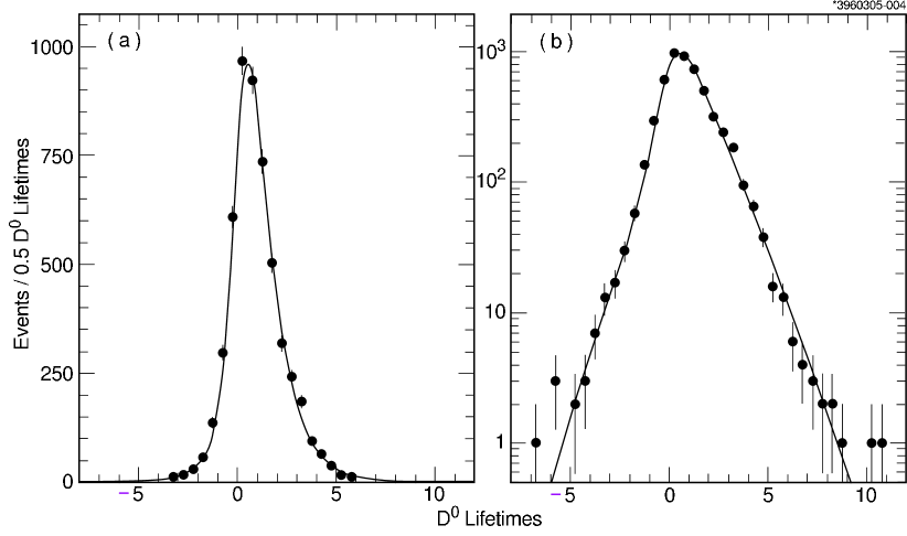
Figure 1: Projection of the results of Fit A onto the ${D^{0}}$ decay time with a) linear and b) logarithmic vertical scale.

The treatment of the background is similar to that of the signal. The total background likelihood is normalized by the background fraction, which is ($1-f_{\rm sig}$). We consider two types of background: background with zero lifetime and background with non-zero lifetime $\tau_{\rm BG}$ normalized by $f_{\tau_{\rm BG}}$. We constrain both backgrounds to have the same resolution function. The model for the resolution function is two Gaussians, with core width $\sigma_{\rm BG}$, misreconstructed width $\sigma_{\rm MisBG}$ and the background fraction $f_{\rm MisBG}$ in the wider Gaussian.

We perform an unbinned maximum likelihood fit to the Dalitz plot which minimizes the function ${\cal F}$ given below

$${\cal F}=\sum_{{D^{0}}}-2\ln{\cal L}+\sum_{{{\overline{D}\vrule width=0.0pt^{0}}}}-2\ln{\cal\overline{L}}\,,$$ (24)

where ${\cal L}$ and ${\cal\overline{L}}$ are defined as in Ref. ourcpvdalitz using ${\cal M}$ and ${\cal\overline{M}}$ as defined in Eqs. Search for ${D^{0}}\!-\!{\overline{D}\vrule width=0.0pt^{0}}$ Mixing in the Dalitz Plot Analysis of ${D^{0}}\to K_{S}^{0}\pi^{+}\pi^{-}$ and Search for ${D^{0}}\!-\!{\overline{D}\vrule width=0.0pt^{0}}$ Mixing in the Dalitz Plot Analysis of ${D^{0}}\to K_{S}^{0}\pi^{+}\pi^{-}$ convolved with the resolution function described above. Simplified Monte Carlo studies indicate that our fit procedure is unbiased and the statistical errors as determined by the fit are accurate.

Our standard fit to the data, described above, is referred to as Fit A. Fit B is identical to Fit A except $CP$ conservation ($\epsilon=0$, $\phi=0$) is assumed. The ${D^{0}}$ and ${\overline{D}\vrule width=0.0pt^{0}}$ sub-samples are fit independently in Fit C1 and Fit C2, respectively. Fit C1 and Fit C2 are identical to Fit B.

Fit A has 35 free parameters; ten resonances and the non-resonant contribution correspond to ten relative amplitudes and ten relative phases, signal fraction and mis-tag fraction, four signal decay time parameters, five background decay time parameters, two mixing parameters and two $CP$-violating parameters. The results for $x$, $y$, $\epsilon$ and $\phi$ are in Table 1 and are consistent with the absence of both ${D^{0}}\!-\!{\overline{D}\vrule width=0.0pt^{0}}$ mixing and $CP$ violation. The one-dimensional, 95% confidence intervals are determined by an increase in negative log likelihood ($-2\ln{\cal L}$) of 3.84 units. All other fit variables are allowed to vary to distinct, best-fit values. The amplitude and phase, $a_{j}$ and $\delta_{j}$, for all fits in Table 1, are consistent with our “no mixing” result ourdalitz . The projection of the results of Fit A onto the ${D^{0}}$ decay time is shown in Fig 1.

Table 1: Results of the Dalitz-plot vs decay time fit of the ${D^{0}}\!\to\!K^{0}_{S}\pi^{+}\pi^{-}$. Fit A allows both ${D^{0}}\!-\!{\overline{D}\vrule width=0.0pt^{0}}$ mixing and $CP$ violation. Fit B is the $CP$-conserving fit, $\epsilon=0$ and $\phi=0$. Fit C1 (C2) is the fit to the ${D^{0}}$ (${\overline{D}\vrule width=0.0pt^{0}}$) sub-sample. The errors shown for Fit A and Fit B are statistical, experimental systematic and modeling systematic respectively and the 95% confidence intervals include systematic uncertainty. The errors for Fit C1 and Fit C2 are statistical only.

Parameter	Best Fit	1-Dimensional 95% C.L.
Fit A a	Most General Fit
$x$ (%)	$\hphantom{-}2.6^{+3.8}_{-9.0}\pm 0.4\pm 0.4$	$|x|<9.8\%$
$y$ (%)	$-0.3\!^{+4.0}_{-4.6}\pm 0.8\pm 0.4$	$|y|<9.5\%$
$\epsilon\hphantom{(\%)}$	$-0.3\pm 0.5$
$\phi$ (o)	$\hphantom{-.}42\pm 78$
Fit B a	$CP$-conserving fit
$x$ (%)	$\hphantom{-}1.9^{+3.2}_{-3.3}\pm 0.4\pm 0.4$	(-4.7:8.6)
$y$ (%)	$-1.4\pm 2.4\pm 0.8\pm 0.4$	(-6.1:3.5)
Fit C1 a	${D^{0}}$ sub-sample
$x$ (%)	$\hphantom{-}3.3^{+5.0}_{-4.8}$	(-6.1:13.5)
$y$ (%)	$-2.8\!^{+3.6}_{-3.7}$	(-10.2:4.2)
Fit C2 a	${\overline{D}\vrule width=0.0pt^{0}}$ sub-sample
$x$ (%)	$\hphantom{-}0.6^{+5.7}_{-8.6}$	(-16.0:11.5)
$y$ (%)	$-0.3\!^{+6.9}_{-3.1}$	(-6.6:13.0)

We find the parameters describing the signal decay time, $f_{\rm sig}=(97.1\pm 0.8)\%$, $\tau_{\rm sig}=402\pm 6$ fs, $S_{\rm Sig}=1.13\pm 0.02$, $\sigma_{\rm MisSig}=735\pm 155$ fs, $(1-f_{\rm MisSig})=(96.9\pm 1.5)\%$ and the parameters describing the background time, $f_{\tau_{\rm BG}}=(100\pm 1)\%$, $\tau_{\rm bg}=94\pm 59$ fs, $(1-f_{\rm MisBG})=(87\pm 11)\%$, $\sigma_{\rm BG}=197\pm 39$ fs, $\sigma_{\rm MisBG}=1116\pm 321$ fs. The scale factor $S_{\rm Sig}$, although not consistent with unity, is comparable to results from other CLEO lifetime analyses which include Ref. CLEOy ; cleokpi ; dlife .

We evaluate a contour in the two-dimensional plane of $y$ versus $x$ that contains the true value of $x$ and $y$ at 95% confidence level (C.L.) without assumption regarding the relative strong phase between ${D^{0}}$ and ${\overline{D}\vrule width=0.0pt^{0}}\to K^{0}_{S}\pi^{+}\pi^{-}$. We determine the contour around our best-fit values where the $-2\ln{\cal L}$ has increased by 5.99 units. All fit variables other than $x$ and $y$ are allowed to vary to distinct, best-fit values at each point on the contour. The contour for Fit A is shown in Fig. 2. On the axes of $x$ and $y$, these contours fall slightly outside the one-dimensional intervals listed in Table 1, as expected. The maximum excursion of the contour of Fit A (Fit B) from the origin corresponds to a 95% C.L. limit on the mixing rate of $R_{M}<0.84\%$ ($R_{M}<0.55\%$).

We take the sample variance of $x$, $y$, $\epsilon$ and $\phi$ from the nominal result compared to the results in the series of fits described below as a measure of the experimental systematic and modeling systematic uncertainty.

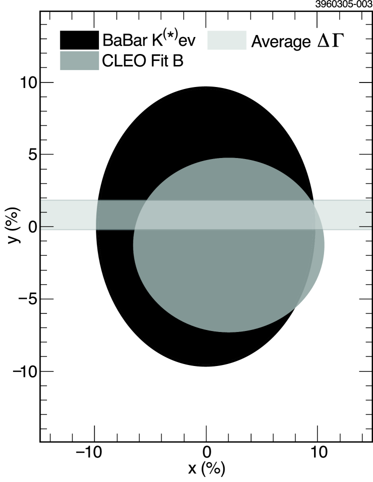
Figure 2: Allowed regions in the plane of $y$ versus $x$. No assumption is made regarding $\delta_{K^{0}_{S}\pi^{+}\pi^{-}}$. The two-dimensional 95% allowed regions from our Fit B (light shaded region) is shown. The allowed region for $\Delta\Gamma$ is the average of the $y_{CP}$ CLEOy ; Belley results. Also shown is the limit from ${D^{0}}\!\to\!K^{(*)}\ell\nu$ from BABAR babarsl . All results are consistent with the absence of mixing. The limits from CLEO cleokpi and BABAR BABARkpi from $D\to K\pi$ have similar sensitivity to Fit B. The 95% allowed regions (not shown) are circles of radius 5.8% and 5.7%, respectively, when assumptions regarding $\delta_{K\pi}$ are removed. The 95% allowed region from Belle bellekpi also from $D\to K\pi$ is more restrictive - a circle of radius 3.0%.

We consider systematic uncertainties from experimental sources and from the decay model separately. Our general procedure is to change some aspect of our fit and interpret the change in the values of the mixing and $CP$-violating parameters in the non-standard fit relative to our nominal fit as an estimate of the systematic uncertainty. Contributions to the experimental systematic uncertainties arise from our model of the background, the efficiency, the event selection criteria, and biases due to experimental resolution as described in Ref. ourdalitz . Additionally, we vary aspects of the decay time parametrization. To estimate the systematic uncertainty regarding the $u\bar{u},d\bar{d},s\bar{s}$ content of the background, we perform fits where the background is forced to be all zero lifetime and all non-zero lifetime. We consider a single or a triple rather than a double Gaussian to model the decay time resolution of the signal and background. We also vary by $\pm 1\sigma$ the fraction of misreconstructed signal $f_{\rm MisSig}$. Finally, we set the scale factor for the measured proper time errors $S_{sig}$ to unity. Variation in the event selection criteria are the largest contribution to the experiment systematic error.

Contributions to the theoretical systematic uncertainties arise from our choices for the decay model for ${D^{0}}\to K_{S}^{0}\pi^{+}\pi^{-}$ as described in Ref. ourdalitz . We also consider the uncertainty arising from our choice of resonances included in the fit. To study the stability of our results with other choices of resonances, we performed fits which included additional resonances to the ones in our standard fit. We compared the result of our nominal fit to a series of fits where each of the resonances, $\sigma$ or $f_{0}(600)$ and $f_{0}(1500)$ which are $CP$-even, and $\rho(1450)$ and $\rho(1700)$ which are $CP$-odd were included one at a time. In the standard fit we enumerate the non-resonant component with the $K^{*}$ resonanaces. We also considered fits where the non-resonant component was considered to be $CP$-even or $CP$-odd. Finally, we consider a fit that includes doubly-Cabibbo suppressed contributions from $K_{0}(1430)$, $K_{2}(1430)$ and $K^{*}(1680)$ constrained to have the same amplitude and phase relative to the corresponding Cabibbo favored amplitude as the $K^{*}(892)$. There is no single dominant contribution to the modeling systematic error.

In conclusion, we have analyzed the time dependence of the three-body decay ${D^{0}}\to K^{0}_{S}\pi^{+}\pi^{-}$ and exploited the interference between intermediate states to limit the mixing parameters $x$ and $y$ without sign or phase ambiguity. Our data are consistent with an absence of both ${D^{0}}\!-\!{\overline{D}\vrule width=0.0pt^{0}}$ mixing and $CP$ violation. The two-dimensional limit in the mixing parameters, $x$ versus $y$, is similar to previous results obtained from the same data sample cleokpi , when assumptions regarding $\delta_{K\pi}$ are removed. We limit $(-4.7\!<\!x\!<\!8.6)\%$ and $(-6.1\!<\!y\!<\!3.5)\%$, at the 95% C.L., with the assumption of $CP$-conservation. We measure the $CP$-violating parameters $\epsilon=-0.3\pm 0.5$ and $\phi=42^{o}\pm 78^{o}$.

We thank Alex Kagan, Yuval Grossman, and Yossi Nir for valuable discussions. We gratefully acknowledge the effort of the CESR staff in providing us with excellent luminosity and running conditions. This work was supported by the National Science Foundation, the U.S. Department of Energy, and the Natural Sciences and Engineering Council of Canada.

References

(1)
R. H. Good et al.,
Phys. Rev. 124 1223 (1961);
M. K. Gaillard, B. W. Lee and J. L. Rosner,
Rev. Mod. Phys. 47, 277 (1975).
(2)
H. Albrecht et al. [ARGUS Collab.],
Phys. Lett. B 192, 245 (1987);
J. L. Rosner, in proceedings of
Hadron 87 (2nd Int. Conf. on Hadron
Spectroscopy) Tsukuba, Japan, April 16-18, 1987,
edited by Y. Oyanagi, K. Takamatsu, and T. Tsuru, KEK, 1987, p. 395.
(3)
See review on page 675 of S. Eidelman et al. [Particle Data Group Collab.],
Phys. Lett. B 592, 1 (2004).
(4)
H. N. Nelson,
in Proc. of the 19th Intl. Symp. on Photon and Lepton
Interactions at High Energy LP99 ed. J.A. Jaros and M.E. Peskin,
SLAC (1999);
S. Bianco, F. L. Fabbri, D. Benson and I. Bigi,
Riv. Nuovo Cim. 26N7, 1 (2003);
A. A. Petrov,
eConf C030603, MEC05 (2003)
[arXiv:hep-ph/0311371];
I. I. Y. Bigi and N. G. Uraltsev,
Nucl. Phys. B 592, 92 (2001);
Z. Ligeti,
AIP Conf. Proc. 618, 298 (2002)
[arXiv:hep-ph/0205316];
A. F. Falk, Y. Grossman, Z. Ligeti and A. A. Petrov,
Phys. Rev. D 65, 054034 (2002);
C. K. Chua and W. S. Hou,
arXiv:hep-ph/0110106.
(5)
M. Leurer, Y. Nir and N. Seiberg,
Nucl. Phys. B 420, 468 (1994);
N. Arkani-Hamed, L. Hall, D. Smith and N. Weiner,
Phys. Rev. D 61, 116003 (2000).
(6)
N. Cabibbo,
Phys. Rev. Lett. 10, 531 (1963);
M. Kobayashi and T. Maskawa, Prog. Theor. Phys. 49 652 (1973).
(7)
L. Wolfenstein,
Phys. Rev. Lett. 51, 1945 (1983).
(8)
S. L. Glashow, J. Iliopoulos and L. Maiani,
Phys. Rev. D 2, 1285 (1970);
R. L. Kingsley, S. B. Treiman, F. Wilczek and A. Zee,
Phys. Rev. D 11, 1919 (1975).
(9)
See review on page 136 of S. Eidelman et al. [Particle Data Group Collab.],
Phys. Lett. B 592, 1 (2004).
(10)
B. Aubert et al. [BABAR Collab.],
Phys. Rev. D 70, 091102 (2004).
(11)
S. E. Csorna et al. [CLEO Collab.],
Phys. Rev. D 65, 092001 (2002).
(12)
K. Abe et al. [Belle Collab.],
Phys. Rev. Lett. 88, 162001 (2002);
B. Aubert et al. [BABAR Collab.],
Phys. Rev. Lett. 91, 121801 (2003);
J. M. Link et al. [FOCUS Collab.],
Phys. Lett. B 485, 62 (2000);
E. M. Aitala et al. [E791 Collab.],
Phys. Rev. Lett. 83, 32 (1999).
(13)
R. Godang et al. [CLEO Collab.],
Phys. Rev. Lett. 84, 5038 (2000).
(14)
B. Aubert et al. [BABAR Collab.],
Phys. Rev. Lett. 91, 171801 (2003).
(15)
K. Abe et al. [Belle Collab.],
Phys. Rev. Lett. 94, 071801 (2005).
(16)
R. H. Dalitz, Phil. Mag. 44, 1068 (1953).
(17)
S. Kopp et al. [CLEO Collab.],
Phys. Rev. D 63, 092001 (2001).
(18)
P. L. Frabetti et al. [E687 Collab.],
Phys. Lett. B 286, 195 (1992);
P. L. Frabetti et al. [E687 Collab.],
Phys. Lett. B 331, 217 (1994).
(19)
H. Muramatsu et al. [CLEO Collab.],
Phys. Rev. Lett. 89, 251802 (2002)
[Erratum-ibid. 90, 059901 (2003)].
(20)
D. M. Asner et al. [CLEO Collab.],
Phys. Rev. D 70, 091101 (2004).
(21)G. Bonvicini et al.,
[CLEO Collab.], Phys. Rev. Lett. 82, 4586 (1999).
(22)
Y. Kubota et al. [CLEO Collab.],
Nucl. Instrum. Meth. A 320, 66 (1992);
T. S. Hill,
Nucl. Instrum. Meth. A 418, 32 (1998).