Search for lepton flavor violating decays $\tau^{-}\rightarrow$ $\ell^{-}\pi^{0},\ell^{-}\eta,\ell^{-}\eta^{\prime}$

Abstract

We have searched for lepton flavor violating semileptonic $\tau^{-}$ decays using a data sample of 153.8 fb^-1 accumulated with the Belle detector at the KEKB $e^{+}e^{-}$ collider. For the six decay modes studied, the observed yield is compatible with the estimated background and the following upper limits are set at the 90% confidence level: $\mathcal{B}(\tau^{-}\rightarrow e^{-}\eta)<2.3\times 10^{-7}$, $\mathcal{B}(\tau^{-}\rightarrow\mu^{-}\eta)<1.5\times 10^{-7}$, $\mathcal{B}(\tau^{-}\rightarrow e^{-}\pi^{0})<1.9\times 10^{-7}$, $\mathcal{B}(\tau^{-}\rightarrow\mu^{-}\pi^{0})<4.1\times 10^{-7}$, $\mathcal{B}(\tau^{-}\rightarrow e^{-}\eta^{\prime})<10\times 10^{-7}$, and $\mathcal{B}(\tau^{-}\rightarrow\mu^{-}\eta^{\prime})<4.7\times 10^{-7}$. These results are 10 to 64 times more restrictive than previous limits.

on leave from ]Nova Gorica Polytechnic, Nova Gorica The Belle Collaboration

I Introduction

Processes with Lepton Flavor Violation (LFV) provide some of the most promising searches for physics beyond the Standard Model (SM). In the charged lepton sector LFV is usually considered for purely leptonic processes such as radiative decays of $\mu$ and $\tau$ hisano or their decays into three charged leptons higgs_mediated . The semileptonic $\tau$ decays $\tau^{-}\to\ell^{-}M^{0}$ (where $\ell^{-}=e^{-},\mu^{-}$ and $M^{0}=\pi^{0},\eta,\eta^{\prime}$) provide another good source of information about possible LFV mechanisms from supersymmetry (SUSY) motivated models Sher ; Brignole:2004ah to models with heavy Dirac neutrinos gonzalez ; ilakovac ; they also allow more general bounds to be placed on the scale of new physics black . Experiments at B factories, where $\tau$ lepton pairs are copiously produced, have substantially increased the sensitivity to LFV decays, bringing it close to various theoretical expectations. Recently we performed a search for the decay $\tau^{-}\to\mu^{-}\eta$ based on a data sample of 84.3 fb^-1 and placed a new upper limit on its branching fraction, $\mathcal{B}(\tau^{-}\to\mu^{-}\eta)<3.4\times 10^{-7}$ res_belle , 28 times better than the previous limit from CLEO cleo and comparable to predictions for some SUSY models Sher ; Brignole:2004ah .

We present here an updated result for $\tau^{-}\rightarrow\mu^{-}\eta$ and new searches for the decay modes $\tau^{-}\rightarrow\mu^{-}\pi^{0}$, $\tau^{-}\rightarrow\mu^{-}\eta^{\prime}$, $\tau^{-}\rightarrow e^{-}\pi^{0}$, $\tau^{-}\rightarrow e^{-}\eta$, and $\tau^{-}\rightarrow e^{-}\eta^{\prime}$, based on a data sample of 153.8 fb^-1, equivalent to 137.2 $\times 10^{6}$ $\tau^{+}\tau^{-}$ pairs, collected at the $\Upsilon(4S)$ resonance with the Belle detector at the KEKB energy-asymmetric $e^{+}e^{-}$ collider KEKB . Due to this much higher integrated luminosity our sensitivity to the decay modes $\tau^{-}\rightarrow\ell^{-}\pi^{0}$ and $\ell^{-}\eta$ is considerably better than in previous searches with MARK II mark , Crystal Ball ball , ARGUS argus and CLEO cleo . The decay modes $\tau^{-}\rightarrow\ell^{-}\eta^{\prime}$ are studied here for the first time. Unless otherwise stated, charge conjugate modes are implied throughout the paper.

The Belle detector is a large-solid-angle magnetic spectrometer that consists of a silicon vertex detector (SVD), a 50-layer central drift chamber (CDC), an array of aerogel threshold Čerenkov counters (ACC), a barrel-like arrangement of time-of-flight scintillation counters (TOF), and an electromagnetic calorimeter (ECL) comprised of CsI(Tl) crystals located inside a superconducting solenoid coil that provides a 1.5 T magnetic field. An iron flux-return located outside of the coil is instrumented to detect $K_{L}^{0}$ mesons and to identify muons (KLM). A more detailed description of the detector can be found in Ref. belle .

For Monte Carlo (MC) studies, the following programs have been used to generate background events: KORALB/TAUOLA tauola for $\tau^{+}\tau^{-}$ processes, QQ qq for $B\bar{B}$ and continuum, BHLUMI bhabha for Bhabha, KKMC kkmc for $\mu^{+}\mu^{-}$ and AAFH aafhb for two-photon processes. We use the following sizes of MC samples: 428 fb^-1 of generic $\tau^{+}\tau^{-}$, 232 fb^-1 of $q\bar{q}$ with $q=u,d,s$, and 160 fb^-1 with $q=c$, 90 fb^-1 of $B\bar{B}$, 119 fb^-1 of $\mu^{+}\mu^{-}$, 9.1 fb^-1 of Bhabha and 205 fb^-1 of two-photon processes. Signal MC is generated by KORALB/TAUOLA. To take a range of possible $\tau^{-}\rightarrow\ell^{-}M^{0}$ production mechanisms into account, we generate events under three different assumptions: uniform angular distribution in the $\tau$ rest frame, $V-A$ interactions, and $V+A$ interactions. We initially assume all $\tau$ decays to have a uniform angular distribution and take the other hypotheses into account later. The Belle detector response is simulated by a GEANT3 geant based program.

II Data Analysis

We follow the same principles of event selection as those in the $\tau^{-}\rightarrow\mu^{-}\eta$ search res_belle . Kinematical variables with a CM superscript are calculated in the center-of-mass frame, and other variables are calculated in the laboratory frame unless otherwise stated. We look for an event with the following particles:

$$\begin{array}[]{c}\left\{\tau^{-}\rightarrow\ell^{-}+M^{0}\right\}+\left\{\tau^{+}\rightarrow({\rm track})^{+}+n\gamma+X\right\},\end{array}$$

where the system $X$ is unobserved. In other words, the events should be consistent with a $\tau^{+}\tau^{-}$ event, in which the $\tau^{-}$ decays into a lepton $\ell^{-}$ and a pseudoscalar meson $M^{0}$ (signal side) and the $\tau^{+}$ decays into a charged track, any number $n\geq 0$ of photons, and one or more neutrinos (tag side). The charged track on the tag side should not be an electron (muon) if the lepton on the signal side is an electron (muon), in order to avoid contamination by Bhabha ($\mu^{+}\mu^{-}$) events. We reconstruct mesons in the following modes: $\pi^{0}\to\gamma\gamma$, $\eta\to\gamma\gamma$, $\eta\to\pi^{+}\pi^{-}\pi^{0}$, $\eta^{\prime}\to\pi^{+}\pi^{-}\eta,\eta\to\gamma\gamma$. When pseudoscalar mesons $M^{0}$ are reconstructed from $\gamma\gamma$, the event has a 1-1 prong configuration. When the $\eta$ is reconstructed from $\pi^{+}\pi^{-}\pi^{0}$, or the $\eta^{\prime}$ is reconstructed in $\eta^{\prime}\rightarrow\pi^{+}\pi^{-}\eta$, $\eta\rightarrow\gamma\gamma$, the event has a 1-3 prong configuration. The signal side thus contains at least two photons in all cases.

For the 1-1 prong selection, the candidate should contain exactly two oppositely charged tracks and two or more photons, two of which form a $\pi^{0}$ or an $\eta$. We require the momentum of each track, $p$, and the energy of each photon, $E_{\gamma}$, to satisfy $p>0.1$ GeV/c and $E_{\gamma}>0.1$ GeV. The tracks and photons are required to be detected within the CDC acceptance, $-0.866$ $<\cos\theta<0.956$. In order to exclude Bhabha, $\mu^{+}\mu^{-}$ and two-photon events, which otherwise contribute a large background, the total visible energy in the CM frame is required to satisfy 5 GeV $<E^{\rm{CM}}_{\rm{total}}<$ 10 GeV. The event is subdivided into two hemispheres by a plane perpendicular to the thrust axis evaluated from all tracks and photons satisfying the above requirements.

The lepton flavor is identified based on likelihood ratios calculated from the response of various subsystems of the detector. For electron identification, the likelihood ratio is defined as $\mathcal{P}_{e}=\mathcal{L}_{e}/(\mathcal{L}_{e}+\mathcal{L}_{x})$, where $\mathcal{L}_{e}$ and $\mathcal{L}_{x}$ are the likelihoods for electron and other flavor hypotheses, respectively, determined using the matching between the position of the charged track trajectory and the cluster position in the ECL, the ratio of the shower energy in the ECL to the momentum measured by the CDC, the shower shape of the cluster in the ECL, specific ionisation ($dE/dx$) in the CDC and the light yield in the ACC eid . For muon identification, the likelihood ratio is $\mathcal{P}_{\mu}=\mathcal{L}_{\mu}/(\mathcal{L}_{\mu}+\mathcal{L}_{K}+\mathcal{L}_{\pi})$, where ${\mathcal{L}}_{\mu}$, ${\mathcal{L}}_{\pi}$, and ${\mathcal{L}}_{K}$ are the likelihoods for the muon, pion and kaon hypotheses respectively, based on the matching quality and penetration depth of associated hits in the KLM muid . For electron candidates $\mathcal{P}_{e}>$ 0.9 is required, identifying electrons with an efficiency $\eta_{e}=(92.4\pm 0.4)$%; the pion fake rate (the probability that a pion is misidentified as an electron) $\kappa_{e}=(0.25\pm 0.02)$%. For muons $\eta_{\mu}=(87.5\pm 0.3)$% and $\kappa_{\mu}=(1.4\pm 0.1)$% are obtained. If the track satisfies ${\mathcal{P}}_{e}>0.6$ or ${\mathcal{P}}_{\mu}>0.6$ on the tag side, i.e. is lepton-like, the constraints $n_{\gamma}^{\rm tag}\leq$ 2 and $p_{e/\mu}^{\rm tag}$ 0.7 GeV/$c$ are applied to suppress events including photons from initial state radiation or beam background. Otherwise, no constraints are applied on the tag side. The lepton flavor identification on the signal side is postponed until the last stage of selection.

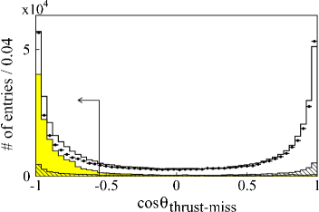
Figure 1: $\cos\theta^{\rm CM}_{\rm thrust-miss}$ distribution for the $\tau^{-}\rightarrow\mu^{-}\eta$ decay mode. The data (points with error bars), total background MC (open histogram), non-$\tau^{+}\tau^{-}$ background MC (hatched histogram), and signal MC (shaded histogram) are shown. The selected region is indicated by the arrow.

Table 1: The resolutions of $M_{\ell^{-}M^{0}}$ and $\Delta E$ for each mode. The “low” or “high” superscript indicates the lower or higher energy side of the peak; $\sigma_{M_{\ell^{-}M^{0}}}$ are in MeV/$c^{2}$ and $\sigma_{\Delta E}$ are in MeV.

Mode	Subdecay mode	$\sigma_{M_{\ell^{-}M^{0}}}^{\rm low}$	$\sigma_{M_{\ell^{-}M^{0}}}^{\rm high}$	$\sigma_{\Delta E}^{\rm low}$	$\sigma_{\Delta E}^{\rm high}$
$\tau^{-}\rightarrow e^{-}\eta$	$\eta\rightarrow\gamma\gamma$	25.8	15.3	79.3	34.7
	$\eta\rightarrow\pi^{+}\pi^{-}\pi^{0}$  ($\pi^{0}\rightarrow\gamma\gamma$)	17.5	9.7	44.2	25.5
$\tau^{-}\rightarrow\mu^{-}\eta$	$\eta\rightarrow\gamma\gamma$	25.7	14.2	57.1	35.2
	$\eta\rightarrow\pi^{+}\pi^{-}\pi^{0}$  ($\pi^{0}\rightarrow\gamma\gamma$)	13.4	9.6	43.2	22.1
$\tau^{-}\rightarrow e^{-}\pi^{0}$	$\pi^{0}\rightarrow\gamma\gamma$	25.7	14.7	69.5	35.2
$\tau^{-}\rightarrow\mu^{-}\pi^{0}$	$\pi^{0}\rightarrow\gamma\gamma$	23.6	14.5	69.8	38.9
$\tau^{-}\rightarrow e^{-}\eta^{\prime}$	$\eta^{\prime}\rightarrow\pi^{+}\pi^{-}\eta$  ($\eta\rightarrow\gamma\gamma$)	22.0	14.0	62.7	26.7
$\tau^{-}\rightarrow\mu^{-}\eta^{\prime}$	$\eta^{\prime}\rightarrow\pi^{+}\pi^{-}\eta$  ($\eta\rightarrow\gamma\gamma$)	18.3	11.7	55.6	25.9

The momentum of a $\pi^{0}$ or $\eta$ meson produced in a two-body $\tau$-decay is on average higher than that of $\pi^{0}/\eta$ mesons from other sources, so that photons from $\pi^{0}$ or $\eta$ are required to have a rather high energy $E_{\gamma}>$ 0.30 (0.22) GeV in the case of $\ell^{-}$ = $e^{-}$($\mu^{-}$). To further reduce the backgrounds, the cosine of the opening angle between $\ell^{-}$ and $\gamma\gamma$ on the signal side must satisfy $0.5<\cos\theta_{\hbox{\scriptsize$\ell^{-}$-$\gamma\gamma$}}<0.95$. When reconstructing an $\eta$ meson candidate, a $\pi^{0}$ veto is applied: defining the resolution-normalized $\pi^{0}$ mass $S^{\pi^{0}}_{\gamma\gamma^{\prime}}=(m_{\gamma\gamma^{\prime}}-0.135~{}\mbox{GeV/}c^{2})/\sigma^{\pi^{0}}_{\gamma\gamma^{\prime}}$, we reject events where a signal-side photon $\gamma$ and a tag-side photon $\gamma^{\prime}$ satisfy $-5<S^{\pi^{0}}_{\gamma\gamma^{\prime}}<+5$; the resolution $\sigma_{\gamma\gamma^{\prime}}^{\pi^{0}}$ is in the range 5–8 MeV/$c^{2}$. This $\pi^{0}$ veto rejects 86% of the BG events while retaining 75% of the signal. To ensure that the missing particles are neutrinos rather than $\gamma$’s or charged particles that fall outside the detector acceptance, we require that the direction of the missing momentum satisfy the condition $-0.866<\cos\theta_{\rm{miss}}<0.956$. Since neutrinos are emitted only on the tag side, the direction of the missing momentum $p_{\rm{miss}}$ should be contained on the tag side. We define the angle $\theta^{\rm CM}_{\rm thrust-miss}$ between the thrust axis of the event (in the signal hemisphere) and the missing momentum vector, and require $\cos\theta_{\rm{thrust-miss}}^{\rm CM}<-0.55$ as shown in Fig. 1. At this level of selection the dominant background is that of $\tau^{+}\tau^{-}$ events (95%) whereas $q\bar{q}$ events and other sources constitute only 5%. The correlation between the missing momentum, $p_{\rm{miss}}$, and the missing mass squared, $m_{\rm{miss}}^{2}$, is used to remove the generic $\tau^{+}\tau^{-}$ and $q\overline{q}$ continuum contributions: $p_{\rm{miss}}>-2.616m^{2}_{\rm{miss}}-0.191$ and $p_{\rm{miss}}>1.0m^{2}_{\rm{miss}}-1$, where $p_{\rm miss}$ is in GeV/$c$ and $m_{\rm miss}$ is in GeV/$c^{2}$.

The yield of signal events is finally determined in the $M_{\ell^{-}M^{0}}$–$\Delta E$ plane, where $M_{\ell^{-}M^{0}}$ is the invariant mass of the $\ell^{-}M^{0}$ system and $\Delta E$ is the difference between the energy of the $\ell^{-}M^{0}$ system and the beam energy in the CM frame. When deciding on our selection criteria, we blinded the signal region $M_{\tau}-5\sigma^{\rm low}_{M_{\ell^{-}M^{0}}}<M_{\ell^{-}M^{0}}<M_{\tau}+5\sigma^{\rm high}_{M_{\ell^{-}M^{0}}}$ and $-0.5$ GeV $<\Delta E<0.5$ GeV. We define sideband regions of $M_{\ell^{-}M^{0}}$ and $\Delta E$ as $M_{\tau}-10\sigma^{\rm low}_{M_{\ell^{-}M^{0}}}<M_{\ell^{-}M^{0}}<M_{\tau}-5\sigma^{\rm high}_{M_{\ell^{-}M^{0}}}$, $M_{\tau}+5\sigma^{\rm low}_{M_{\ell^{-}M^{0}}}<M_{\ell^{-}M^{0}}<M_{\tau}+10\sigma^{\rm high}_{M_{\ell^{-}M^{0}}}$ and $-10\sigma_{\Delta E}^{\rm low}<\Delta E<-0.5$ GeV, 0.5 GeV $<\Delta E<10\sigma_{\Delta E}^{\rm high}$, respectively. The resolutions, $\sigma_{M_{\ell^{-}M^{0}}}^{\rm low/high}$ and $\sigma_{\Delta E}^{\rm low/high}$, of $M_{\ell^{-}M^{0}}$ and $\Delta E$, are evaluated from the distributions of signal MC around the peak using an asymmetric Gaussian shape to account for initial state radiation and ECL energy leakage for photons. In these expressions, $M_{\tau}$ is the central value of the reconstructed $\tau$ mass for signal, evaluated in MC: it is consistent with the known $\tau$ mass within 1.2 – 13.0 MeV for each mode. The resulting resolutions are summarized in Table 1.

The resulting numbers of data and MC events in the $M_{\ell^{-}M^{0}}$–$\Delta E$ sideband region after applying a loose mass requirement for $\pi^{0}/\eta$, $-5<S_{\gamma\gamma}^{\pi^{0}/\eta}<5$, are summarized in Table 2. The $S_{\gamma\gamma}^{\pi^{0}}$ and $S_{\gamma\gamma}^{\eta}$ distributions for the modes with a final state muon are shown in Fig.2 (a) and (b), respectively. Within the statistical uncertainty the sideband data and background MC yields are consistent with each other in all four modes.

At the last stage of the selection, the $\pi^{0}$ or $\eta$ candidate is required to satisfy $-5<S^{\pi^{0}/\eta}_{\gamma\gamma}<3$, where $S^{\pi^{0}}_{\gamma\gamma}$ was defined above, and $S^{\eta}_{\gamma\gamma}=(m_{\gamma\gamma}-0.547~{}\mbox{GeV/}c^{2})/\sigma^{\eta}_{\gamma\gamma}$ with $\sigma^{\eta}_{\gamma\gamma}$ = 11–13 MeV$/c^{2}$. The conditions ${\mathcal{P}}_{e/\mu}>0.9$ and $p>0.7$ GeV/c are imposed on lepton tracks on the signal side. In addition, ${\mathcal{P}}_{e/\mu}<0.6$ is required on the tag side for rejection of Bhabha or $\mu^{+}\mu^{-}$ events.

Table 2: Numbers of remaining events for each mode at the same selection stage as in Fig. 2, prior to final cuts on the signal side (see the text).

Mode	Subdecay mode	$N_{\rm side}^{\rm DATA}$	$N_{\rm side}^{\rm MC}$
$\tau^{-}\rightarrow e^{-}\eta$	$\eta\rightarrow\gamma\gamma$	3	1.47 $\pm$ 0.73
	$\eta\rightarrow\pi^{+}\pi^{-}\pi^{0}$	5	0.34 $\pm$ 0.11
$\tau^{-}\rightarrow\mu^{-}\eta$	$\eta\rightarrow\gamma\gamma$	17	14.4 $\pm$ 3.2
	$\eta\rightarrow\pi^{+}\pi^{-}\pi^{0}$	7	5.2 $\pm$ 3.6
$\tau^{-}\rightarrow e^{-}\pi^{0}$	$\pi^{0}\rightarrow\gamma\gamma$	2	2.2 $\pm$ 0.9
$\tau^{-}\rightarrow\mu^{-}\pi^{0}$	$\pi^{0}\rightarrow\gamma\gamma$	22	25.8 $\pm$ 4.5
$\tau^{-}\rightarrow e^{-}\eta^{\prime}$	$\eta^{\prime}\rightarrow\pi^{+}\pi^{-}\eta$	12	11.6 $\pm$ 2.3
$\tau^{-}\rightarrow\mu^{-}\eta^{\prime}$	$\eta^{\prime}\rightarrow\pi^{+}\pi^{-}\eta$	33	22.9 $\pm$ 3.5

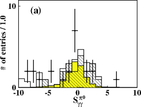
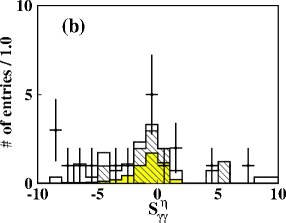
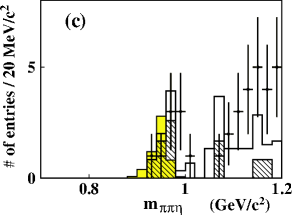
Figure 2: $S_{\gamma\gamma}^{\pi^{0}}$, $S_{\gamma\gamma}^{\eta}$ and $m_{\pi^{+}\pi^{-}\eta}$ distributions for (a) $\tau^{-}\rightarrow\mu^{-}\pi^{0}$, (b) $\tau^{-}\rightarrow\mu^{-}\eta$ and (c) $\tau^{-}\rightarrow\mu^{-}\eta^{\prime}$ decay modes, respectively, prior to final cuts on the signal side (see the text). The data (points with error bars), total background MC (open histogram), non-$\tau^{+}\tau^{-}$ background MC (hatched histogram), and signal MC (shaded histogram, corresponding to the branching fraction of 5$\times$10^-7) are shown.

For $\eta\rightarrow\pi^{+}\pi^{-}\pi^{0}$ and $\eta^{\prime}\rightarrow\pi^{+}\pi^{-}\eta$ decays with $\eta\rightarrow\gamma\gamma$, i.e. 1-3 prong modes, we search for events containing four charged tracks (net charge = 0) and two or more photons. Because of the higher multiplicity compared to the 1-1 prong modes, the detection efficiency becomes smaller. On the other hand, the additional reconstruction constraint in the $\eta/\eta^{\prime}$ decay chain improves the background rejection power. The selection criteria are similar to those in the $\eta\to\gamma\gamma$ case with the differences listed below.

The minimum photon energy $E_{\gamma}$ requirement is reduced from 0.1 GeV to 0.05 GeV, and the tighter conditions for photons from $\pi^{0}/\eta$ are also removed, since the photons from these decay modes have a softer energy distribution compared to that in the 1-1 prong case. At least three tracks and two or more photons are required in the signal hemisphere. One track must be identified as an electron or a muon (${\mathcal{P}}_{{e}/\mu}>$ 0.9), but particle identification is not performed on the other two tracks, at first they are treated as pions. We also require that one $\pi^{0}$ is reconstructed with $-5<S_{\gamma\gamma}^{\pi^{0}}<5$ from the photons in the signal hemisphere. Without any PID for pion candidate tracks on the signal side, possible photon conversions can result in a fake event. In order to remove such a contribution, we examine the effective mass-squared $M^{2}_{ee}$ of any two tracks (to which the electron mass is assigned) in the signal hemisphere. A sharp peak at $M^{2}_{ee}<0.01$ $(\rm{GeV}/c^{2})^{2}$ is seen in the Bhabha MC but not in the signal and generic $\tau^{+}\tau^{-}$ MC’s, and data also exhibit a tiny peak at $M^{2}_{ee}\sim 0$ $(\rm{GeV}/c^{2})^{2}$. To avoid a large reduction of the signal detection efficiency, we impose a requirement on PID in addition to that on $M^{2}_{ee}$: events are rejected which have $M^{2}_{ee}<0.01$ GeV/$c^{2}$ and ${\mathcal{P}}_{e}>0.6$ for one of the two tracks. As a result, 60% of the Bhabha originated events are rejected while the signal efficiency is reduced by 2.3% only. In addition, the following constraints are also required: $p_{\rm{miss}}>-1.5m^{2}_{\rm{miss}}-1.0$ and $p_{\rm{miss}}>0.8m^{2}_{\rm{miss}}-0.2$, where $p_{\rm miss}$ is in GeV/$c$ and $m_{\rm miss}$ is in GeV/$c^{2}$.

The $\pi^{0}$ and $\eta$ from $\gamma\gamma$ are extracted by imposing the conditions $-3<S_{\gamma\gamma}^{\pi^{0}}<3$ and $-5<S_{\gamma\gamma}^{\eta}<3$, respectively. The requirements ${\mathcal{P}}_{e/\mu}>0.9$ and $p>0.7$ GeV/c are imposed on the tracks on the signal side as in the 1-1 prong case. After applying the above conditions as well as the requirements on the invariant mass 1.3 GeV/$c^{2}$ $<M_{\ell^{-}M^{0}}<$ 2.0 GeV/$c^{2}$, energy difference $-1.0$ GeV $<\Delta E<$ 0.5 GeV and a loose requirement on $\eta$ ($\eta^{\prime}$) mass $m_{\pi^{+}\pi^{-}\pi^{0}}<0.65$ GeV/$c^{2}$ ($m_{\pi^{+}\pi^{-}\eta}<1.2$ GeV/$c^{2}$), we obtain the resulting number of data and MC events summarized in Table 2. The $m_{\pi^{+}\pi^{-}\eta}$ distribution of the mode with a final state muon after these requirements is shown in Fig. 2 (c).

Again, agreement between sideband data and background MC is observed within the statistical uncertainty, except for the decay mode $\tau^{-}\rightarrow e^{-}\eta$, $\eta\rightarrow\pi^{+}\pi^{-}\pi^{0}$. Since in this mode PID has better rejection power of hadronic background than in the modes with a final state muon, the $\eta$ candidates should be mostly fake ones. In fact, four of the remaining five data events are in the $\eta$ mass sideband regions and thus will be rejected at the last stage by the tighter $\eta$ and $\eta^{\prime}$ mass requirement 0.5260 GeV/$c^{2}<m_{\pi^{+}\pi^{-}\pi^{0}}<$ 0.5656 GeV/$c^{2}$ and 0.9027 GeV/$c^{2}<m_{\pi^{+}\pi^{-}\eta}<$ 0.9798 GeV/$c^{2}$, corresponding to the $\pm 3\sigma$ regions, where the resolutions are estimated from signal MC.

III BG Estimations and Branching Fractions

The signal detection efficiency for each mode is evaluated by using signal MC. We take an elliptically shaped signal region in the $M_{\ell^{-}M^{0}}$–$\Delta E$ plane with a signal acceptance, $\Omega$, of 90%, which is more sensitive than a box shaped signal region. To obtain the highest sensitivity, all geometrical parameters of the ellipse, such as the position of the center, the orientation, and the length of the major and minor axes, are determined to minimize its area with the constraint on the acceptance to be 90%.

As explained in the previous section, an analysis of the background MC distributions shows that they agree well with data in the sideband regions. We also confirmed that no peaking background structure, which mimics the signal, is observed in the signal region.

The expected number of background events ($b_{0}$) in the signal elliptical region is estimated from sideband data events as follows: for the decay modes $\tau^{-}\rightarrow\mu^{-}\eta~{}(\eta\rightarrow\gamma\gamma)$, $\tau^{-}\rightarrow\mu^{-}\pi^{0}$ and $\tau^{-}\rightarrow\mu^{-}\eta^{\prime}$, we assume that the background distribution is described by a polynomial function in $M_{\ell^{-}M^{0}}$ and a Gaussian function in $\Delta E$ over the $\pm 10\sigma$ region. We determine the shape of the function by fitting to the MC events including the blinded region with its normalization from the data sideband. Moreover, taking into account the uncertainties from assuming the background distribution, we evaluate $b_{0}$ for these modes by another method: we assume a flat distribution over the $\pm 10\sigma$ region of $M_{\ell^{-}M^{0}}$ and the regions $-0.4$ GeV $<\Delta E<0.20$ GeV, $-0.5$ GeV $<\Delta E<0.33$ GeV and $-0.4$ GeV $<\Delta E<0.20$ GeV for the $\mu^{-}\eta~{}(\eta\rightarrow\gamma\gamma)$, $\mu^{-}\pi^{0}$, and $\mu^{-}\eta^{\prime}$ modes, respectively. The differences between the values evaluated by the first and the second method, which are 21%, 10% and 49%, respectively, are treated as an additional uncertainty. For the other five decay modes, we evaluate $b_{0}$ from sideband data events by simply assuming a flat distribution over $\pm 10\sigma$ region of $M_{\ell^{-}M^{0}}$–$\Delta E$ plane, since the remaining number of events is too small to determine the background shape by fitting to those events. The uncertainty on $b_{0}$ is quite large ($\leq$ 100%), particularly in the electron modes, because the number of events remaining in the sideband region is very small. For $\tau^{-}\rightarrow e^{-}\pi^{0}$, there are no events in the sidebands, and we set $b_{0}=0.0^{+0.4}_{-0.0}$ where the error is calculated by assuming 2.44 events in the sideband. The resultant $b_{0}$ are listed in Table 3.

Table 3: Results of the final event selection for the individual modes: $\epsilon$ is the detection efficiency, $\mathcal{B}_{M^{0}}$ is the branching fraction for the $M^{0}$ decay, $N^{\rm DATA}_{\rm side}$ and $N^{\rm MC}_{\rm side}$ are the numbers of events in sideband regions for data and MC, respectively, $b_{0}$ is the expected number of background events, $s$ is the observed number of signal events and $s_{0}$ is the upper limit on the number of signal events.

Mode	Subdecay	$\epsilon$	${\mathcal{B}}_{M^{0}}$	$N^{\rm{DATA}}_{\rm{side}}$	$N^{\rm{MC}}_{\rm{side}}$	$b_{0}$	$s$	$s_{0}$
	mode	(%)	(%)	(ev.)	(ev.)	(ev.)	(ev.)	(ev.)
$\tau^{-}\rightarrow e^{-}\eta$	$\eta\rightarrow\gamma\gamma$	5.68	39.43	2	0	$0.23\pm 0.16$	0	2.3
	$\eta\rightarrow\pi^{+}\pi^{-}\pi^{0}$	6.84	22.6	1	0	$0.23\pm 0.23$	0	2.2
$\tau^{-}\rightarrow\mu^{-}\eta$	$\eta\rightarrow\gamma\gamma$	8.03	39.43	9	$9.2\pm 2.3$	$3.9\pm 1.5$	1	1.4
	$\eta\rightarrow\pi^{+}\pi^{-}\pi^{0}$	7.15	22.6	2	$0.8\pm 0.3$	$0.60\pm 0.42$	0	1.9
$\tau^{-}\rightarrow e^{-}\pi^{0}$	$\pi^{0}\rightarrow\gamma\gamma$	4.70	98.798	0	$0.7\pm 0.7$	$0.0^{+0.4}_{-0.0}$	0	2.4
$\tau^{-}\rightarrow\mu^{-}\pi^{0}$	$\pi^{0}\rightarrow\gamma\gamma$	6.36	98.798	16	$12.5\pm 2.7$	$3.0\pm 0.9$	5	6.9
$\tau^{-}\rightarrow e^{-}\eta^{\prime}$	$\eta^{\prime}\rightarrow\pi^{+}\pi^{-}\eta$	8.51	17.5	2	$0.8\pm 0.3$	$0.28\pm 0.20$	1	4.2
$\tau^{-}\rightarrow\mu^{-}\eta^{\prime}$	$\eta^{\prime}\rightarrow\pi^{+}\pi^{-}\eta$	8.41	17.5	5	$5.5\pm 1.9$	$0.94\pm 0.60$	0	1.6

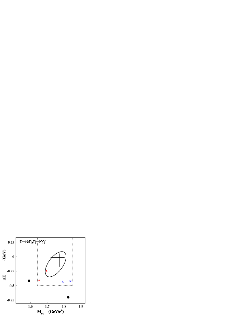
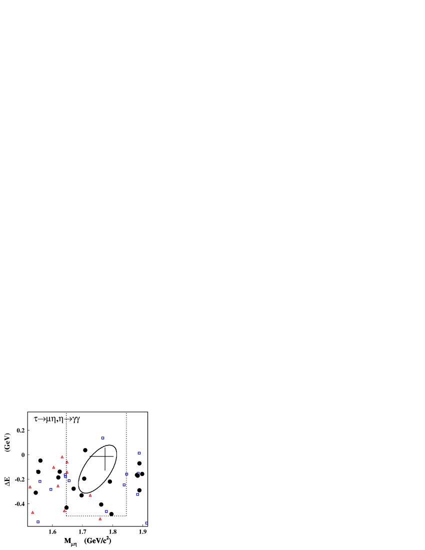
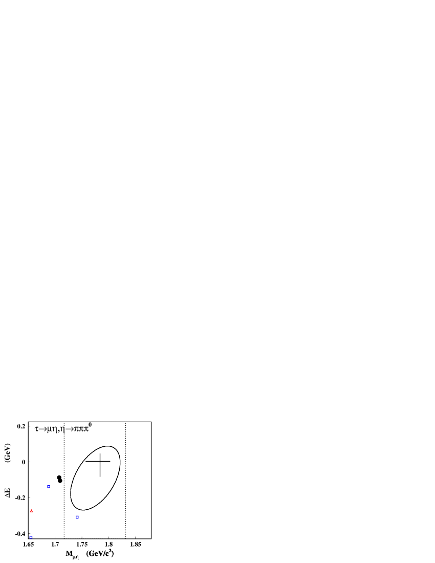
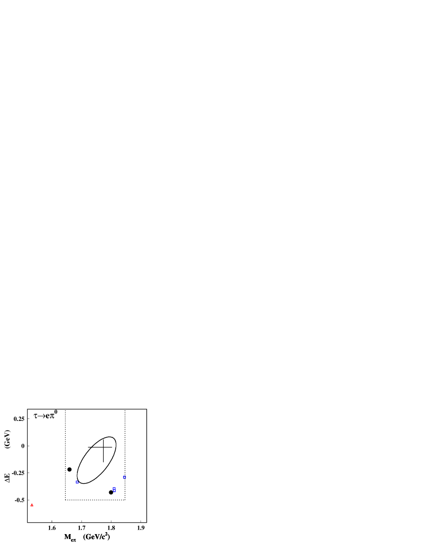
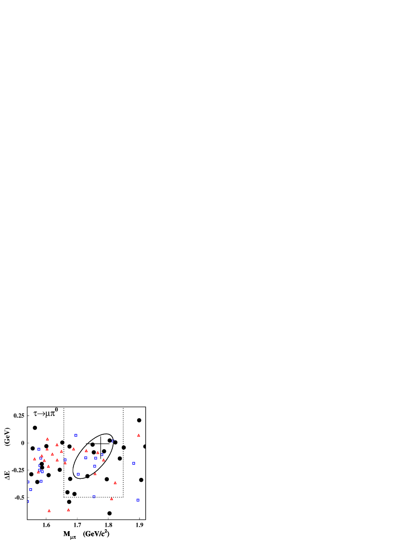
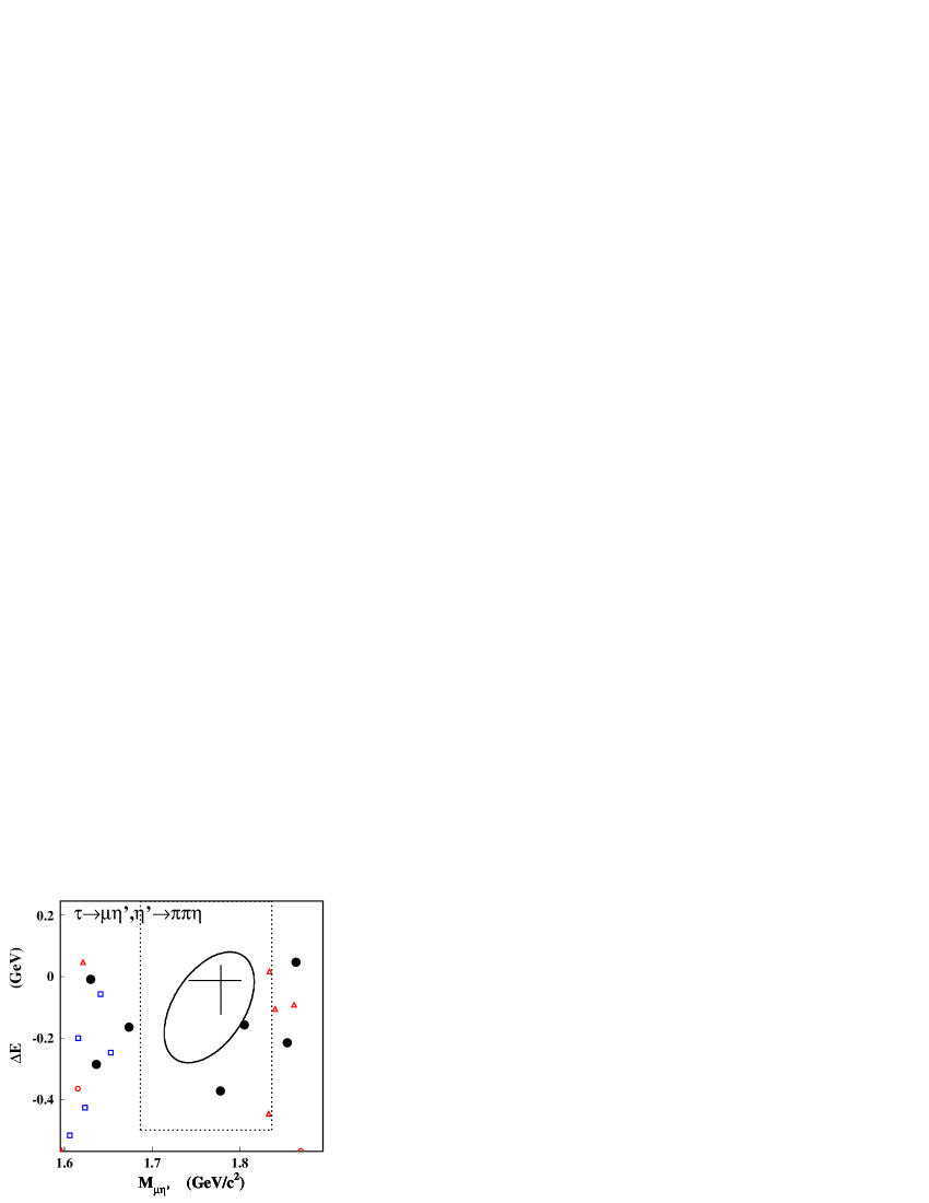
Figure 3: The distribution of remaining events over the $\pm 10\sigma$ region in the $M_{\ell^{-}M^{0}}-\Delta E$ plane after opening the blinded region. The ellipse is the signal region that has a signal acceptance of $\Omega=90\%$. The blinded regions $\pm 5\sigma$ in $M_{\ell^{-}M^{0}}$ and $\pm 0.5$ GeV in $\Delta E$ are indicated by the dotted lines. The cross indicates the $\pm 2\sigma$ $M_{\ell^{-}M^{0}}$ and $\Delta E$ ranges. Various symbols show events from 428 fb^-1 of generic $\tau^{+}\tau^{-}$ MC ($\Box$), 232 fb^-1 of $q\bar{q}$ MC with $q=u,d,s$ ($\vartriangle$), 160 fb^-1 with $q=c$ ($\circ$), 205 fb^-1 of two-photon MC ($\blacktriangledown$), and data ($\bullet$).

After opening the blinded region, we find one event in both the $\tau^{-}\rightarrow e^{-}\eta^{\prime}$ and $\tau^{-}\rightarrow\mu^{-}\eta$ modes, and five events in the $\tau^{-}\rightarrow\mu^{-}\pi^{0}$ mode, however, no events are found for the other modes in the elliptical signal region. Figure 3 shows the $M_{\ell^{-}M^{0}}$–$\Delta E$ plot for the individual modes. The resultant numbers of events $s$ are compared to the expected background $b_{0}$ in Table 3: good agreement can be observed.

Following the Feldman-Cousins method FC , we calculate the upper limit $s_{0}$ on the number of signal events at the 90% confidence level (C.L.) for all modes, as listed in Table 3. These values take only statistical errors into account.

The branching fraction at the 90% C.L. is obtained from the following formula,

$${\mathcal{B}}(\tau^{-}\rightarrow\ell^{-}M^{0})=\frac{s_{0}}{2~{}\epsilon~{}{\mathcal{B}}_{M^{0}}N_{\tau\tau}},$$ (1)

where $\epsilon$ is the detection efficiency for the individual modes, ${\mathcal{B}}_{M^{0}}$ is the branching fraction for the $M^{0}$ decay, and $N_{\tau\tau}=137.2\times 10^{6}$ is the number of produced $\tau$-pairs at 153.8 fb^-1 luminosity, with the cross section of $e^{+}e^{-}\rightarrow\tau^{+}\tau^{-}$ at the $\Upsilon(4S)$ resonance $\sigma_{\tau\tau}=0.892\pm 0.002$ nb calculated by KKMC kkmc . The values of $\epsilon$ and $\mathcal{B}_{M^{0}}$ for each mode are listed in Table 3. Systematic uncertainties due to the background estimate $b_{0}$, and uncertainties on $2\epsilon\mathcal{B}_{M_{0}}N_{\tau\tau}$, are taken into account by inflating the value of $s_{0}$, as discussed below.

Table 4: Systematic uncertainties in %.

Mode   $\tau^{-}\rightarrow$	$e^{-}\eta,$	$e^{-}\eta,$	$\mu^{-}\eta,$	$\mu^{-}\eta,$	$e^{-}\pi^{0}$	$\mu^{-}\pi^{0}$	$e^{-}\eta^{\prime}$	$\mu^{-}\eta^{\prime}$
	$\eta\rightarrow\gamma\gamma$	$\eta\rightarrow 3\pi$	$\eta\rightarrow\gamma\gamma$	$\eta\rightarrow 3\pi$
Track recon.	2.0	2.0	2.0	2.0	2.0	2.0	2.0	2.0
$M^{0}$ recon.	2.0	4.0	2.0	4.0	2.0	2.0	4.0	4.0
$\pi^{0}$ veto	5.5	–	5.5	–	–	–	5.5	5.5
$e$ ID	1.0	1.0	–	–	1.0	–	1.0	–
$\mu$ ID	–	–	2.0	2.0	–	2.0	–	2.0
Trigger	0.5	0.1	0.2	0.1	0.7	0.4	0.1	0.1
Beam background	2.3	2.1	2.3	2.1	2.3	2.3	2.1	2.1
Luminosity	1.4	1.4	1.4	1.4	1.4	1.4	1.4	1.4
$\mathcal{B}_{M^{0}}$	0.7	1.8	0.7	1.8	–	–	3.4	3.4
MC stat.	1.4	1.7	1.1	1.6	0.9	0.8	1.2	1.1
MC models	0.5	0.5	0.5	0.5	0.5	0.5	0.5	0.5
Total	7.0	5.8	7.2	6.0	4.2	4.5	8.4	8.6

The systematic uncertainties on the detection sensitivity, $2\epsilon{\mathcal{B}}_{M^{0}}N_{\tau\tau}$, arise from the track reconstruction efficiency (1.0% for each track) of the tag side track and the signal side lepton; $\pi^{0}$, $\eta$ and $\eta^{\prime}$ reconstruction efficiency which includes the uncertainties in the tracking efficiency for charged pions (2.0%) and the $\pi^{0}$ or $\eta$ reconstruction efficiency (2.0%); $\pi^{0}$ veto for $\tau^{-}\rightarrow\ell^{-}\eta$ and $\ell^{-}\eta^{\prime}$ modes (5.5%); electron or muon identification efficiency (1.0% for electron, 2.0% for muon); trigger efficiency (0.1–0.7%); beam background effect (2.1% for 1-1 prong, 2.3% for 1-3 prong events); luminosity (1.4%); branching fraction of $\pi^{0}$, $\eta$, and $\eta^{\prime}$ (Ref. pdg ); signal MC statistics (0.8–1.7%) and signal MC models (0.5%). Table  4 lists these separate contributions as well as the resulting systematic uncertainties obtained by adding all the components in quadrature. The dominant contributions, $\pi^{0}$, $\eta$ and $\eta^{\prime}$ reconstruction efficiencies, $\pi^{0}$ veto efficiency and beam background effect, are estimated as follows. The contribution of reconstruction efficiencies for pseudoscalar mesons is evaluated from the efficiency ratios for data and MC samples using $\eta\rightarrow\gamma\gamma$ and $\eta\rightarrow 3\pi^{0}$ decays. The $\pi^{0}$ veto contribution is also evaluated by the efficiency ratio of data and MC, where the $\pi^{0}$ veto efficiency is estimated from the difference of $\eta$ reconstruction efficiencies with and without the $\pi^{0}$ veto. The beam background effect is estimated from data that is taken by the random trigger at the same time as the normal data taking. We initially assumed a uniform angular distribution of $\tau$ decays for the signal MC. Its possible nonuniformity was taken into account by comparing the uniform case with those assuming $V-A$ and $V+A$ interactions spin , which result in maximum possible variations. This effect contributes 0.5% shown in the “MC models” line of Table 4.

The treatment of systematic uncertainties depends on the estimated background $b_{0}$. In cases where $b_{0}<1.0$, except for $\tau^{-}\rightarrow\mu^{-}\eta^{\prime}$, we set $b_{0}$ to $0.0\pm 0.0$ to obtain a conservative upper limit. We use the POLE program pole to recalculate $s_{0}$ including systematic uncertainties on both $b_{0}$ and the detection sensitivity, assuming Gaussian errors Cous . The upper limits then obtained from equation (1) are summarized in Table 5.

Table 5: Upper limits on branching fractions.

Mode	Subdecay mode	U.L. of ${\mathcal{B}}$ @ 90% C.L.
$\tau^{-}\rightarrow e^{-}\eta$	$\eta\rightarrow\gamma\gamma$	$4.0\times 10^{-7}$
	$\eta\rightarrow\pi^{+}\pi^{-}\pi^{0}$	$5.8\times 10^{-7}$
$\tau^{-}\rightarrow e^{-}\eta$	combined	$2.4\times 10^{-7}$
$\tau^{-}\rightarrow\mu^{-}\eta$	$\eta\rightarrow\gamma\gamma$	$2.3\times 10^{-7}$
	$\eta\rightarrow\pi^{+}\pi^{-}\pi^{0}$	$5.5\times 10^{-7}$
$\tau^{-}\rightarrow\mu^{-}\eta$	combined	$1.5\times 10^{-7}$
$\tau^{-}\rightarrow e^{-}\pi^{0}$	$\pi^{0}\rightarrow\gamma\gamma$	$1.9\times 10^{-7}$
$\tau^{-}\rightarrow\mu^{-}\pi^{0}$	$\pi^{0}\rightarrow\gamma\gamma$	$4.1\times 10^{-7}$
$\tau^{-}\rightarrow e^{-}\eta^{\prime}$	$\eta^{\prime}\rightarrow\pi^{+}\pi^{-}\eta$	$10\times 10^{-7}$
$\tau^{-}\rightarrow\mu^{-}\eta^{\prime}$	$\eta^{\prime}\rightarrow\pi^{+}\pi^{-}\eta$	$4.7\times 10^{-7}$

IV Discussion

One can see from Table 5 that for the $\tau^{-}\rightarrow e^{-}\eta^{\prime}$ and $\tau^{-}\rightarrow\mu^{-}\eta^{\prime}$ modes, the resulting 90% C.L. upper limits are ${\mathcal{B}}(\tau^{-}\rightarrow e^{-}\eta^{\prime})<10\times 10^{-7}$ and ${\mathcal{B}}(\tau^{-}\rightarrow\mu^{-}\eta^{\prime})<4.7\times 10^{-7}$; these are the first experimental limits on these modes. For the $\tau^{-}\rightarrow e^{-}\eta$ and $\tau^{-}\rightarrow\mu^{-}\eta$ modes, the results from two different final states, $\eta\rightarrow\gamma\gamma$ and $\eta\rightarrow\pi^{+}\pi^{-}\pi^{0}$, are combined. The resulting 90% C.L. upper limits for these two modes and $\tau^{-}\rightarrow e^{-}\pi^{0}$ and $\tau^{-}\rightarrow\mu^{-}\pi^{0}$ are ${\mathcal{B}}(\tau^{-}\rightarrow e^{-}\eta)<2.4\times 10^{-7}$, ${\mathcal{B}}(\tau^{-}\rightarrow\mu^{-}\eta)<1.5\times 10^{-7}$, ${\mathcal{B}}(\tau^{-}\rightarrow e^{-}\pi^{0})<1.9\times 10^{-7}$ and ${\mathcal{B}}(\tau^{-}\rightarrow\mu^{-}\pi^{0})<4.1\times 10^{-7}$ and improve upon the previous CLEO measurements by a factor of 34, 64, 20 and 10, respectively.

We can restrict the allowed parameter space for $m_{A}$–$\tan\beta$, using the relationship derived by M. Sher Sher in a seesaw MSSM with a specific mass texture:

$${\mathcal{B}}(\tau^{-}\!\!\rightarrow\mu^{\!-}\eta)=0.84\times 10^{-6}\!\times\!\left(\frac{\rm{tan}\beta}{60}\right)^{6}\left(\frac{100~{}\rm{GeV}}{m_{A}}\right)^{4},$$ (2)

where $m_{A}$ is the pseudoscalar Higgs mass and $\rm{tan}\beta$ is the ratio of the vacuum expectation values $(\langle H_{u}\rangle/\langle H_{d}\rangle)$, as shown in Fig. 4, where our boundary is indicated for the 90% C.L by the shaded region. Figure 4 also shows the 95% C.L. constraints from our experiment with a dashed line and high energy collider experiments at LEP LEP and CDF Tevatron . Our experiment has a sensitivity competitive with that of the CDF experiment which searched for $pp\rightarrow A/\phi b\overline{b}\rightarrow b\overline{b}b\overline{b}$ reactions, where $\phi$ is a CP-even neutral Higgs state and $A$ is a CP-odd state in the MSSM.

The improved sensitivity to rare $\tau$ lepton decays achieved in this work can also be used to constrain the parameters of models with heavy Dirac neutrinos gonzalez ; ilakovac . In these models the expected branching ratios of various LFV decays are evaluated in terms of combinations of the model parameters. These combinations, denoted $y_{\tau e}$ and $y_{\tau\mu}$ for $\tau$ decays involving an electron and a muon, respectively, can vary from 0 to 1. Our $\tau^{-}\to e^{-}\pi^{0}$ result sets a 90% C.L. upper limit $y_{\tau e}<0.26$, the most restrictive bound on this quantity. The corresponding limit from our $\tau^{-}\to\mu^{-}\pi^{0}$ result is $y_{\tau\mu}<0.87$: a somewhat better bound $y_{\tau\mu}<0.65$ can be set from the $\tau^{-}\to\mu^{-}\mu^{+}\mu^{-}$ decay based on the experimental limits from BaBar babar_3l and Belle belle_3l .

In summary, using a data sample of 153.8 fb^-1 collected with the Belle detector we obtained new upper limits on the branching fractions of semileptonic LFV $\tau^{-}$ decays involving pseudoscalar mesons $\pi^{0},~{}\eta$ and $\eta^{\prime}$. They range from $1.5\times 10^{-7}$ to $10\times 10^{-7}$ for the six decay modes studied and are 10 to 64 times more restrictive than previous limits.

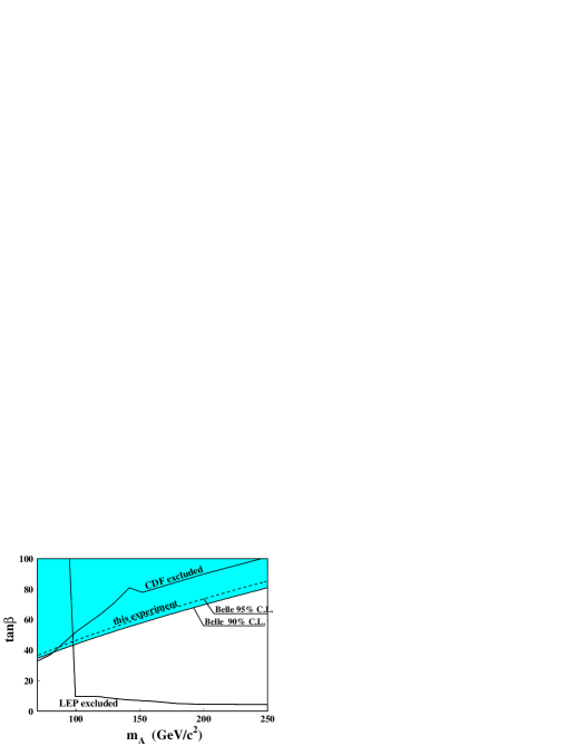
Figure 4: Experimentally excluded $m_{A}-\tan\beta$ parameter space. The 90% C.L. result of this experiment on $\mathcal{B}(\tau^{-}\rightarrow\mu^{-}\eta)$ using the relation (2) is indicated by the shaded region together with the 95% C.L. regions excluded by this experiment (dashed line), LEP LEP and the CDF Tevatron ; pdg .

V Acknowledgements

We thank the KEKB group for the excellent operation of the accelerator, the KEK cryogenics group for the efficient operation of the solenoid, and the KEK computer group and the National Institute of Informatics for valuable computing and Super-SINET network support. We are grateful to A. Ilakovac for fruitful discussions. We acknowledge support from the Ministry of Education, Culture, Sports, Science, and Technology of Japan and the Japan Society for the Promotion of Science; the Australian Research Council and the Australian Department of Education, Science and Training; the National Science Foundation of China under contract No. 10175071; the Department of Science and Technology of India; the BK21 program of the Ministry of Education of Korea and the CHEP SRC program of the Korea Science and Engineering Foundation; the Polish State Committee for Scientific Research under contract No. 2P03B 01324; the Ministry of Science and Technology of the Russian Federation; the Ministry of Higher Education, Science and Technology of the Republic of Slovenia; the Swiss National Science Foundation; the National Science Council and the Ministry of Education of Taiwan; and the U.S. Department of Energy.

References

(1)
J. Hisano, T. Moroi, K. Tobe and M. Yamaguchi, Phys. Rev. D 53, 2442 (1996).
(2)
K.S. Babu and C. Kolda, Phys. Rev. Lett. 89, 241802 (2002);
A. Dedes, J. Ellis and M. Raidal, Phys. Lett. B 549, 159 (2002).
(3) A. Brignole and A. Rossi,
Nucl. Phys. B 701, 3 (2004).
(4) M. Sher, Phys. Rev. D 66, 057301 (2002).
(5) M.C. Gonzalez-Garcia and J.W.F. Valle,
Mod. Phys. Lett. A 7, 477 (1992).
(6) A. Ilakovac, Phys. Rev. D 62, 036010 (2000).
(7) D. Black et al., Phys. Rev. D 66, 053002 (2002).
(8) Y. Enari et al. (Belle Collaboration),
Phys. Rev. Lett. 93, 081803 (2004).
(9) G. Bonvicini et al. (CLEO Collaboration),
Phys. Rev. Lett. 79, 1221 (1997).
(10) S. Kurokawa and E. Kikutani,
Nucl. Instr. Meth. A 499, 1 (2003), and other papers
included in this Volume.
(11) K.G. Hayes et al. (MARK II Collaboration),
Phys. Rev. D 25, 2869 (1982).
(12) S. Keh et al. (Crystal Ball Collaboration),
Phys. Lett B 212, 123 (1988).
(13) H. Albrecht et al. (ARGUS Collaboration),
Z. Phys. C 55, 179 (1992).
(14) A. Abashian et al. (Belle Collaboration),
Nucl. Instr. Meth. A 479, 117 (2002).
(15) S. Jadach and Z.Wa̧s,
Comp. Phys. Commun. 85, 453 (1995).
(16)
QQ is an event generator developed by the CLEO Collaboration and
described in http://www.lns.cornell.edu/public/CLEO/soft/QQ.
It is based on
the LUND Monte Carlo for jet fragmentation and physics described in
T. Sjöstrand, Comput. Phys. Commun. 39 367 (1986),
T. Sjöstrand and M.Bengtsson, Comput. Phys. Commun. 43 367 (1987).
(17) S. Jadach, E. Richter-Wa̧s, B.F.L. Ward and Z. Wa̧s,
Comp. Phys. Commun. 70, 305 (1992).
(18) S. Jadach, B.H.L. Ward and Z. Wa̧s,
Comp. Phys. Commun. 130, 260 (2000).
(19) F.A. Berends, P.H. Daverveldt and R. Kleiss,
Comp. Phys. Commun. 40, 285 (1986).
(20) R. Brun et al., GEANT 3.21 CERN Report No. DD/EE/84-1, 453.
(21)
K. Hanagaki et al., Nucl. Instr. Meth. A 485, 490 (2002).
(22)
A. Abashian et al., Nucl. Instr. Meth. A 491, 69 (2002).
(23) G. J. Feldman and R. D. Cousins,
Phys. Rev. D 57, 3873 (1998).
(24) S. Eidelman et al., Phys. Lett. B 592, 1 (2004).
(25) R. Kitano and Y. Okada, Phys. Rev. D 63, 113003 (2001).
(26) J. Conrad et al., Phys. Rev. D 67, 012002 (2003).
(27) R. Cousins and V. Highland,
Nucl. Instr. Meth. A 320, 331 (1992).
(28) LEP Higgs Working Group,
http://lephiggs.web.cern/ LEPHIGGS/papers/ Note 2001-04.
(29) T. Affolder et al. (CDF Collaboration),
Phys. Rev. Lett. 86, 4472 (2001).
(30) B. Aubert et al. (BaBar Collaboration),
Phys. Rev. Lett. 92, 121801 (2004).
(31) Y. Yusa et al. (Belle Collaboration),
Phys. Lett. B 589, 103 (2004).