Observation of $p\overline{p}\pi^{0}$ and $p\overline{p}\eta$ in $\psi^{\prime}$ decays

Abstract

The processes $\psi^{\prime}\rightarrow p\overline{p}\pi^{0}$ and $\psi^{\prime}\rightarrow p\overline{p}\eta$ are studied using a sample of $14\times 10^{6}$ $\psi^{\prime}$ decays collected with the Beijing Spectrometer at the Beijing Electron-Positron Collider. The branching fraction of $\psi^{\prime}\rightarrow p\overline{p}\pi^{0}$ is measured with improved precision as $(13.2\pm 1.0\pm 1.5)\times 10^{-5}$, and $\psi^{\prime}\rightarrow p\overline{p}\eta$ is observed for the first time with a branching fraction of $(5.8\pm 1.1\pm 0.7)\times 10^{-5}$, where the first errors are statistical and the second ones are systematic.

I Introduction

There are some long-standing puzzles in the decays of vector charmonia, in particular the “$\rho\pi$ puzzle” between $\psi^{\prime}$ and $J/\psi$ decays and the possible large charmless decay branching fraction of the $\psi^{\prime\prime}$. Following the suggestion in Ref. rosnersd that the small $\psi^{\prime}\rightarrow\rho\pi$ branching fraction is due to the cancellation of the $S$- and $D$-wave matrix elements in $\psi^{\prime}$ decays, it was pointed out that all $\psi^{\prime}$ decay channels should be affected by the same $S$- and $D$-wave mixing scheme, and thus, in general, the ratios between the branching fractions of $\psi^{\prime}$ and $J/\psi$ decay into the same final states may have values different from the “12% rule”, expected for pure $1S$ and $2S$ states wymcharmless . This scenario also predicts $\psi^{\prime\prime}$ decay branching fractions since $\psi^{\prime\prime}$ would also be a mixture of $S$- and $D$-wave charmonia, and it was suggested that many $J/\psi$ and $\psi^{\prime}$, as well as $\psi^{\prime\prime}$, decays should be measured to test this. For the channels that have been measured, $\psi^{\prime}$ decays are found to be either suppressed (like vector-pseudoscalar, vector-tensor), or enhanced (like $K^{0}_{S}K^{0}_{L}$), or obey the 12% rule (like baryon-antibaryon pairs). In this paper, we analyze three-body decays of $\psi^{\prime}$ into a $p\overline{p}$ pair and a $\pi^{0}$ or $\eta$.

The $J/\psi$ and $\psi^{\prime}$ decays into $p\overline{p}\pi^{0}$ and $p\overline{p}\eta$ are expected to be dominated by two-body decays involving excited nucleon states. These states play an important role in the understanding of nonperturbative QCD role1 ; role2 ; role3 ; role4 . However, our knowledge on $N^{*}$ resonances, based on $\pi N$ and $\gamma N$ experiments pdg , is still very limited and imprecise. Studies of $N^{*}$ resonances have also been performed using $J/\psi$ events collected at the Beijing Electron-Positron Collider (BEPC) zounstar ; jpsippeta ; pnbarpi , which provides a new method for probing $N^{*}$ physics. Recently, based on 58 million $J/\psi$ events collected by BEijing Spectrometer (BESII), a new $N^{*}$ peak with a mass at around 2065 MeV/$c^{2}$ was observed pnbarpi . This may be one of the “missing $N^{*}$ states” around 2 GeV/$c^{2}$ that have been predicted by the quark model in many of its forms role2 ; model1 ; model2 . However, due to its large mass, the production of this $N^{*}(2065)$ in $J/\psi$ decays is rather limited in phase space, and a similar search for it in $\psi^{\prime}$ decays, which has a larger phase space available may be helpful, although the production rate may be small due to the large decay rates for $\psi^{\prime}$ into final states with charmonium.

In a recent paper zhangzx , it is predicted that $p\overline{p}$ in $\psi^{\prime}\rightarrow p\overline{p}\pi^{0}$ may form iso-vector bound states near threshold. These states can also be searched for.

Experimentally, $\psi^{\prime}\rightarrow p\overline{p}\pi^{0}$ was studied by Mark-II in 1983, with only 9 events observed markii , and the branching ratio was found to be $(1.4\pm 0.5)\times 10^{-4}$. $\psi^{\prime}\rightarrow p\overline{p}\eta$ has not been observed before.

II Detector and data samples

The data used in this analysis were taken with the BESII detector at the BEPC storage ring at a center-of-mass energy corresponding to $M_{\psi^{\prime}}$. The data sample corresponds to a total of ($14.0\pm 0.6)\times 10^{6}$ $\psi^{\prime}$ decays, as determined from inclusive hadronic events pspscan .

BES is a conventional solenoidal magnet detector that is described in detail in Refs. bes ; bes2 . A 12-layer vertex chamber (VTC) surrounding the beam pipe provides trigger information. A forty-layer main drift chamber (MDC), located radially outside the VTC, provides trajectory and energy loss ($dE/dx$) information for charged tracks over $85\%$ of the total solid angle. The momentum resolution is $\sigma_{p}/p=0.017\sqrt{1+p^{2}}$ ($p$ in $\hbox{GeV}/c$), and the $dE/dx$ resolution for hadron tracks is $\sim 8\%$. An array of 48 scintillation counters surrounding the MDC measures the time-of-flight (TOF) of charged tracks with a resolution of $\sim 200$ ps for hadrons. Radially outside the TOF system is a 12 radiation length, lead-gas barrel shower counter (BSC). This measures the energies of electrons and photons over $\sim 80\%$ of the total solid angle with an energy resolution of $\sigma_{E}/E=22\%/\sqrt{E}$ ($E$ in GeV). Outside of the solenoidal coil, which provides a 0.4 Tesla magnetic field over the tracking volume, is an iron flux return that is instrumented with three double layers of counters that identify muons of momentum greater than 0.5 GeV/$c$.

Monte Carlo (MC) simulation is used for the determination of the invariant mass resolution and detection efficiency, as well as the study of background. The simulation of the BESII detector is Geant3 based, where the interactions of particles with the detector material are simulated. Reasonable agreement between data and Monte Carlo simulation is observed simbes in various channels tested including $e^{+}e^{-}\rightarrow(\gamma)e^{+}e^{-}$, $e^{+}e^{-}\rightarrow(\gamma)\mu^{+}\mu^{-}$, $J/\psi\rightarrow p\overline{p}$ and $\psi^{\prime}\rightarrow\pi^{+}\pi^{-}J/\psi$, $J/\psi\rightarrow\ell^{+}\ell^{-}$ $(\ell=e,\mu)$.

The signal channels $\psi^{\prime}\rightarrow p\overline{p}\pi^{0}$, $\pi^{0}\to 2\gamma$ and $\psi^{\prime}\rightarrow p\overline{p}\eta$, $\eta\to 2\gamma$ are generated with a phase space generator, giving similar $p\pi$, $\overline{p}\pi$, $p\eta$, and $\overline{p}\eta$ mass distributions to those observed in data. For $\pi^{0}$ and $\eta$ channels, 100 000 events each are simulated. To study possible background in our analysis, 20 000 $\psi^{\prime}\rightarrow\pi^{0}\pi^{0}J/\psi$, $J/\psi\rightarrow p\overline{p}$, 20 000 $\psi^{\prime}\rightarrow\pi^{0}\pi^{0}p\overline{p}$, and 30 000 $\psi^{\prime}\rightarrow\gamma\chi_{cJ}$, $\chi_{cJ}\rightarrow\gamma J/\psi$, $J/\psi\rightarrow p\overline{p}$ ($J=0,1,2$) events are generated.

III Event Selection

The final states in which we are interested contain two photons and two charged tracks. The number of charged tracks is required to be two with net charge zero. Each track should have good quality in track fitting and satisfy $|\cos\theta|<0.8$, where $\theta$ is the polar angle of the track measured by the MDC.

A neutral cluster in the BSC is considered to be a photon candidate when the angle between the nearest charged track and the cluster in the $xy$ plane is greater than $15^{\circ}$, the first hit appears in the first five layers of the BSC (about six radiation lengths of material), and the angle between the cluster development direction in the BSC and the photon emission direction in $xy$ plane is less than $37^{\circ}$. Two or three photon candidates are allowed in an event, but the two with the largest energies are selected as $\pi^{0}$ or $\eta$ decay candidates, and both of them are required to have energy greater than 60 MeV.

A likelihood method is used for discriminating pion, kaon, proton, and antiproton tracks. For every charged track, we define an estimator as $E^{i}=P^{i}/\sum_{i}P^{i}$, where $P^{i}$ is the probability under the hypothesis of being type $i$, $i=3,4,5$ for $\pi,K$ and p or $\overline{p}$ hypotheses, respectively, and $P^{i}=\prod_{j}P_{j}^{i}(x_{j})$. Here $P_{j}^{i}$ is the probability density for the hypothesis of type $i$, associated to the discriminating variable $x_{j}$. Discriminating variables used for each charged track are time of flight in the TOF (TOF-T) and the pulse height in the MDC ($dE/dx$). By definition, pion, kaon, proton, and antiproton tracks have corresponding $E^{i}$ values near one. In this analysis, both tracks are required to have $E^{5}>0.6$.

A four-constraint (four momentum conservation) kinematic fit is made with the two charged tracks and two photon candidates; the confidence level of the $\chi^{2}$ fit is required to be greater than 1%. A similar fit assuming the two charged tracks are $K^{+}K^{-}$ is also performed, and the $\chi^{2}$ of $\psi^{\prime}\rightarrow\gamma\gamma p\overline{p}$ should be smaller than that of $\psi^{\prime}\rightarrow\gamma\gamma K^{+}K^{-}$.

The scatter plot of the $p\overline{p}$ invariant mass versus that of the two photon candidates for events satisfying the above selection criteria is shown in Fig. 1(a). The two bands with $m_{\gamma\gamma}$ values near 0.135 GeV/$c^{2}$ and 0.547 GeV/$c^{2}$ are $\psi^{\prime}\rightarrow p\overline{p}\pi^{0}$, $\pi^{0}\to 2\gamma$ and $\psi^{\prime}\rightarrow p\overline{p}\eta$, $\eta\to 2\gamma$ candidates, respectively. The band corresponding to $p\overline{p}$ mass around 3.1 GeV/$c^{2}$ is from $\psi^{\prime}\rightarrow\gamma\chi_{cJ}$, $\chi_{cJ}\rightarrow\gamma J/\psi$, $J/\psi\rightarrow p\overline{p}$ ($J=0,1,2$), and $\psi^{\prime}\rightarrow\eta J/\psi$, $J/\psi\rightarrow p\overline{p}$. The broadly distributed background in the figure is due mainly to $\psi^{\prime}\rightarrow\pi^{0}\pi^{0}J/\psi$, $J/\psi\rightarrow p\overline{p}$. Fig. 1(b) shows the corresponding Monte Carlo distribution of these background channels, using branching fractions measured by previous experiments pdg . To remove these background events, we require $|m_{p\overline{p}}-3.097|>$ 1.5 $\sigma$ for $\gamma\gamma$ invariant mass ($m_{\gamma\gamma}$) smaller than 0.4 GeV/$c^{2}$, and $m_{p\overline{p}}<3.2-0.3m_{\gamma\gamma}$ for $m_{\gamma\gamma}$ larger than 0.4 GeV/$c^{2}$, where $\sigma\approx 0.011$ GeV/$c^{2}$ is the $p\overline{p}$ invariant mass resolution as estimated from Monte Carlo simulation of $\psi^{\prime}\rightarrow\gamma\chi_{cJ}$. After the above selection, the $\gamma\gamma$ invariant mass distributions are shown in Figs. 2(a) and (c), where clear $\pi^{0}$ and $\eta$ signals are observed.

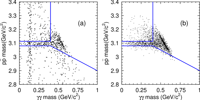
Figure 1: Scatter plots of $p\overline{p}$ invariant mass versus $\gamma\gamma$ invariant mass before removing $J/\psi$ background. (a) is from data and (b) is from Monte Carlo simulated $\psi^{\prime}\rightarrow\gamma\chi_{cJ}$, $\chi_{cJ}\rightarrow\gamma J/\psi$, $J/\psi\rightarrow p\overline{p}$ ($J=0,1,2$), $\psi^{\prime}\rightarrow\eta J/\psi$, $J/\psi\rightarrow p\overline{p}$, and $\psi^{\prime}\rightarrow\pi^{0}\pi^{0}J/\psi$, $J/\psi\rightarrow p\overline{p}$ events. The lines show the selection criterion described in the text.

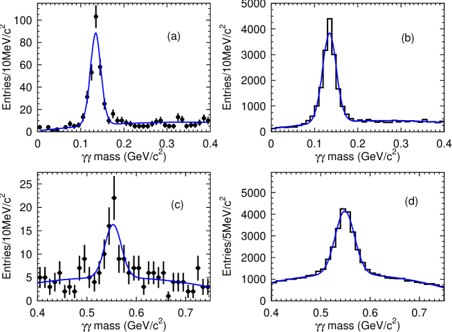
Figure 2: Invariant mass distributions of $\gamma\gamma$ from the selected $\psi^{\prime}\rightarrow\gamma\gamma p\overline{p}$ candidate events in data and in Monte Carlo simulation described in Section V: (a) $p\overline{p}\pi^{0}$ data, (b) $p\overline{p}\pi^{0}$ Monte Carlo simulation, (c) $p\overline{p}\eta$ data, and (d) $p\overline{p}\eta$ Monte Carlo simulation. The curves show the best fit to the distributions.

The same analysis is performed on a MC sample of 14 M inclusive $\psi^{\prime}$ decays generated with Lundcharm lundcharm . It is found that the remaining backgrounds are mainly from $\psi^{\prime}\rightarrow\pi^{0}\pi^{0}p\overline{p}$, many via resonances such as $f_{0}$ and $f_{2}$. Some other decay channels of $\psi^{\prime}$ with three photons such as $\psi^{\prime}\rightarrow\gamma\chi_{c0},\chi_{c0}\rightarrow\overline{p}\Delta^{+},\Delta^{+}\rightarrow\pi^{0}p$ are also observed. Since there are no branching fractions available for normalization of these channels, we do not try to simulate all possible background channels. Instead, in our fit to the $\gamma\gamma$ mass distributions, we approximate the background shape by a smooth curve as predicted by the inclusive MC sample.

IV Fits to the $\gamma\gamma$ mass distributions

The $\gamma\gamma$ invariant mass distribution of candidates is not described well by a simple Gaussian, but by the sum of multiple Gaussians with different standard deviations, which depend on the momentum of the $\pi^{0}$ or $\eta$. The analysis of the $\pi^{0}$ signal is done using five different momentum bins, which are fit with multiple Gaussians for the signal and a second order polynomial for the background. Summing up all the fits yields the curve in Fig. 2(a), and the total number of $\psi^{\prime}\rightarrow p\overline{p}\pi^{0}$ events is found to be $256\pm 18$, with the error determined from the fit.

The number of $\psi^{\prime}\rightarrow p\overline{p}\eta$ events is even more limited than $\psi^{\prime}\rightarrow p\overline{p}\pi^{0}$, and we do not do the fit in $\eta$ momentum bins. Instead the $\gamma\gamma$ invariant mass spectrum is fit with a single Gaussian for the signal plus a second-order polynomial for the background. In the fit, the mass resolution is fixed to 14.3 MeV/$c^{2}$, which is determined from Monte Carlo simulation but calibrated using the $\pi^{0}$ signal in the $p\overline{p}\pi^{0}$ fit. The fit is shown in Fig. 2(c), and the number of events is found to be $44.8^{+8.7}_{-8.4}$. The $\eta$ mass from the fit, $(552.4\pm 3.2)$ MeV/$c^{2}$, agrees well with the world average pdg . The statistical significance of the $p\overline{p}\eta$ signal is estimated to be 6.1$\sigma$ by comparing the likelihoods with and without the signal in the fit.

V Resonance analysis and efficiency

In order to determine the selection efficiency, it is necessary to know the intermediate states in the decays for Monte Carlo simulation. Figs. 3(a) and (c) are the Dalitz plots for $\psi^{\prime}\rightarrow p\overline{p}\pi^{0}$ and $\psi^{\prime}\rightarrow p\overline{p}\eta$ after requiring the $\gamma\gamma$ invariant mass to be consistent with a $\pi^{0}$ (0.11 GeV/$c^{2}<m_{\gamma\gamma}<0.16$ GeV/$c^{2}$) or $\eta$ (0.53 GeV/$c^{2}<m_{\gamma\gamma}<0.57$ GeV/$c^{2}$). In these figures, the requirement on the $p\overline{p}$ mass is removed to see the effect of the backgrounds remaining from $\psi^{\prime}\rightarrow\eta J/\psi$, $\psi^{\prime}\rightarrow\pi^{0}\pi^{0}J/\psi$, and $\psi^{\prime}\rightarrow\gamma\chi_{cJ}$ in the lower left of the Dalitz plots. These two figures differ significantly from phase space. However, the data samples here are too small to perform a partial wave analysis.

Figure 3: Dalitz plots for $\psi^{\prime}\rightarrow p\overline{p}\pi^{0}$ and $\psi^{\prime}\rightarrow p\overline{p}\eta$. (a) and (b) are for $\psi^{\prime}\rightarrow p\overline{p}\pi^{0}$ data and the mixed Monte Carlo sample, respectively, and (c) and (d) are for $\psi^{\prime}\rightarrow p\overline{p}\eta$ data and the mixed Monte Carlo sample, respectively.

In the MC simulation, $N^{*}(1535)\overline{p}+c.c.$ and $R(2000)\pi^{0}$ were used in the $p\overline{p}\pi^{0}$ mode and $N^{*}(1535)\overline{p}+c.c.$ and $R(2000)\eta$ in $p\overline{p}\eta$ mode, where $R(2000)$ is a state representing the accumulation of the events near $p\overline{p}$ mass threshold with

$$p\overline{N}^{*}(1535):\overline{p}N^{*}(1535):\pi^{0}R(2000)=2:2:1$$

for the $p\overline{p}\pi^{0}$ mode, and

$$p\overline{N}^{*}(1535):\overline{p}N^{*}(1535):\eta R(2000)=5:5:3$$

for the $p\overline{p}\eta$ mode, and $N^{*}$, $\pi^{0}$, and $\eta$ only decay into desired final states. The MC simulations of the Dalitz plots are shown in Figs. 3(b) and (d). The agreement between data and MC simulation is reasonable.

Fig. 4 shows the angular distributions for our selected data samples as well as the mixed MC samples, where $\theta$ is the polar angle of the proton measured in the $\psi^{\prime}$ rest frame, $\theta^{*}$ and $\phi^{*}$ are the polar and azimuthal angles of the anti-proton in the rest frame of $\overline{p}\pi$ (or $\overline{p}\eta$). The simulations are similar to data, although not perfect. Using the same analysis as used for data on the two mixed MC samples, with proper fractions of background added to the $\gamma\gamma$ mass distributions, yields efficiencies of $(14.04\pm 0.14)\%$ for $\psi^{\prime}\rightarrow p\overline{p}\pi^{0}$ and $(14.00\pm 0.20)\%$ for $\psi^{\prime}\rightarrow p\overline{p}\eta$.

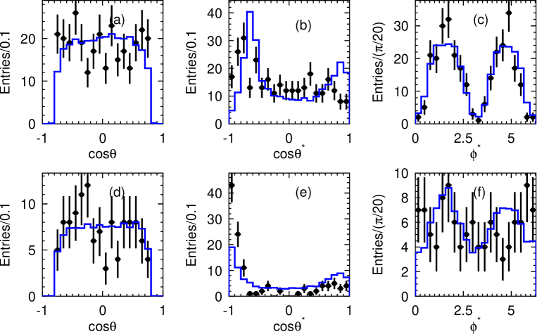
Figure 4: Angular distributions of selected $\psi^{\prime}\rightarrow p\overline{p}\pi^{0}$ (top) and $\psi^{\prime}\rightarrow p\overline{p}\eta$ (bottom) events. The dots with error bars are data and the histograms are MC simulation (normalized to the same number of events). The first through third columns are $\cos\theta$, $\cos\theta^{*}$ and $\phi^{*}$ distributions.

VI Systematic Errors

The systematic errors, whenever possible, are evaluated with pure data samples that are compared with the MC simulations. Table 1 lists the systematic errors from all sources. Adding all these errors in quadrature, the total percentage errors are 11.2% and 11.6% for $\pi^{0}p\overline{p}$ and $\eta p\overline{p}$ respectively. The detailed analyses are described in the following.

Table 1: Summary of systematic errors. Numbers common to the two channels are only listed once.

Source	$\pi^{0}p\overline{p}$ (%)	$\eta p\overline{p}$ (%)
MC statistics	1.0	1.4
Photon ID	1.1
Photon efficiency	4
$\pi^{0}(\eta)$ reconstruction	2.0
Tracking and particle ID	2.6	2.8
Fit to mass spectrum	4.5	5.3
Decay dynamics	5.9
Kinematic fit	5
Number of $\psi^{\prime}$	4
Trigger efficiency	0.5
${\cal B}[\pi^{0}(\eta)\rightarrow\gamma\gamma]$	0.0	0.7
Total Systematic error	11.2	11.6

VI.1 Photon ID

The fake photon multiplicity distributions and energy spectra for both data and Monte Carlo simulation for $\psi^{\prime}\rightarrow p\overline{p}$ are shown in Fig. 5. For this decay channel, the Monte Carlo simulates slightly less fake photons than data, while it simulates the energy spectra reasonably well.

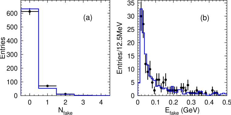
Figure 5: Fake photon multiplicity distributions (left) and fake photon energy spectra (right) for $\psi^{\prime}\rightarrow p\overline{p}$ data (dots with error bars) and Monte Carlo simulation (histogram).

Using a toy Monte Carlo simulation, we found that for $(97.10\pm 0.32)\%$ of the cases, the energies of both real photons are greater than those of the fake ones from data, while for Monte Carlo simulation, the corresponding fraction is $(97.78\pm 0.15)\%$. A factor of $(0.993\pm 0.004)$ is found between data and Monte Carlo. We do not apply a correction to the MC efficiency; instead, we take 1.1% as the systematic error of photon identification (ID).

VI.2 Photon detection efficiency

The simulation of the photon detection efficiency is studied using $J/\psi\rightarrow\pi^{+}\pi^{-}\pi^{0}$ events with one photon missing in the kinematic fit and examining the detector response in the missing photon direction lism . The Monte Carlo simulates the detection efficiency of data within 2% for each photon in the full energy range. Since we have two photons, 4% is taken as the systematic error of the photon detection efficiency.

VI.3 $\pi^{0}$ and $\eta$ reconstruction

The $\pi^{0}$ reconstruction efficiency is studied by comparing the opening angle between the two photons between data and MC simulation in different $\pi^{0}$ momentum ranges using $J/\psi\rightarrow p\overline{p}\pi^{0}$ and $J/\psi\rightarrow\pi^{+}\pi^{-}\pi^{0}$ samples selected from BES $J/\psi$ data. Fig. 6 shows the comparison for $\pi^{0}$ momentum between 0.5 GeV/$c$ and 0.6 GeV/$c$, the agreement at small opening angle shows the simulation of the $\pi^{0}$ reconstruction efficiency is good. By reweighting the difference between data and MC simulation in all momentum bins with the $\pi^{0}$ momentum spectrum in $\psi^{\prime}\rightarrow p\overline{p}\pi^{0}$, the overall correction factor to the MC simulation is determined to be ($98.8\pm 0.8$)%, and 2.0% is then taken as the systematic error due to the $\pi^{0}$ reconstruction.

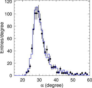
Figure 6: Comparison of the $\gamma\gamma$ opening angle ($\alpha$) distributions for $\pi^{0}$ from $J/\psi\rightarrow\pi^{+}\pi^{-}\pi^{0}$ with momentum between 0.5 GeV/$c$ and 0.6 GeV/$c$. Dots with error bars are data, and the histogram is Monte Carlo simulation. The distributions are normalized to the number of events with $\alpha>28^{\circ}$.

The angle between the two photons emitted from the $\eta$ is generally much greater than that from the $\pi^{0}$. As a conservative estimation, the uncertainty for $\eta$ reconstruction is also taken to be 2.0%.

VI.4 MDC tracking and particle ID efficiency

The efficiencies for protons and antiprotons that enter the detector being reconstructed and identified are measured using samples of $J/\psi\rightarrow\pi^{+}\pi^{-}p\overline{p}$ and $\psi^{\prime}\rightarrow\pi^{+}\pi^{-}J/\psi,J/\psi\rightarrow p\overline{p}$ events, which are selected using kinematic fit and particle ID for three tracks, allowing one proton or antiproton at a time to be missing in the fit. The efficiency is determined by how often a proton (or antiproton) is found in the direction of the missing track, it varies from 80% to around 95% with increasing momentum, and the MC simulates data rather well, except for proton or antiproton momenta less than 0.5 GeV/$c$, where the nuclear interaction cross section of particles with the detector material is very large.

The net difference between data and MC simulation is found to be $1.001\pm 0.025$ for $\psi^{\prime}\rightarrow p\overline{p}\pi^{0}$, and $1.010\pm 0.018$ for $\psi^{\prime}\rightarrow p\overline{p}\eta$. The errors together with the differences from unity will be considered as systematic errors, that is, 2.6% and 2.8% for $\psi^{\prime}\rightarrow p\overline{p}\pi^{0}$ and $\psi^{\prime}\rightarrow p\overline{p}\eta$, respectively.

VI.5 Fit range and background shape

The background shape in fitting the $\gamma\gamma$ mass distributions is changed from a second order polynomial to a first order one, and the fit range is changed, to determine the uncertainties due to the fitting for the $p\overline{p}\pi^{0}$ and $p\overline{p}\eta$ channels. Different ways for choosing the $\pi^{0}$ momentum bins or fitting the $\pi^{0}$ signal without binning yields differences in the branching fraction less than 3% for the $p\overline{p}\pi^{0}$ channel. Adding all these in quadrature, 4.5% and 5.3% are taken as the systematic error due to the fit.

VI.6 Decay dynamics

Table 2 shows efficiencies determined with different MC samples; different decay dynamics result in different efficiencies. While the mixed Monte Carlo samples with $N^{*}$ and possible $p\overline{p}$ intermediate states are used in the determination of final selection efficiencies, the differences between the mixed samples and the phase space generator are taken as systematic errors due to the lack of the precise knowledge of the decay dynamics to be used in the MC generator. The differences are found to be 2.1% for $\psi^{\prime}\rightarrow p\overline{p}\pi^{0}$ and 5.9% for $\psi^{\prime}\rightarrow p\overline{p}\eta$. The larger difference (5.9%) will be taken as the systematic error for both due to the uncertainty of the generator for both channels. It should be noted that the differences between these two MC samples in the angular distributions are large compared with those observed in Fig. 4; thus the errors quoted cover the differences in the angular distribution simulation also.

Table 2: Efficiencies determined with different MC samples.

Channel	$p\overline{p}\pi^{0}$ (%)	$p\overline{p}\eta$ (%)
Only $N^{*}(1535)$	13.04	12.71
Only $R(2000)$	18.43	18.40
Mixed sample	$14.04\pm 0.14$	$14.00\pm 0.20$
Phase space	14.37	14.83

VI.7 Other systematic errors

The uncertainty due to the kinematic fit is extensively studied using many channels which can be selected cleanly without using a kinematic fit gpp ; wangz ; fangss ; vt . It is found that the MC simulates the kinematic fit efficiency at the 5% level for almost all the channels tested. We take 5% as the systematic error due to the kinematic fit.

The results reported here are based on a data sample corresponding to a total number of $\psi^{\prime}$ decays, $N_{\psi^{\prime}}$, of $(14.0\pm 0.6)\times 10^{6}$, as determined from inclusive hadronic events pspscan . The uncertainty of the number of $\psi^{\prime}$ events, 4%, is determined from the uncertainty in selecting the inclusive hadrons.

The trigger efficiency is around 100% with an uncertainty of 0.5%, as estimated from Bhabha and $e^{+}e^{-}\rightarrow\mu^{+}\mu^{-}$ events. The systematic errors on the branching fractions used are obtained from the Particle Data Group (PDG) pdg tables directly.

VII Conclusion and Discussion

The branching fractions of $\psi^{\prime}\rightarrow p\overline{p}\pi^{0}$ and $\psi^{\prime}\rightarrow p\overline{p}\eta$ are calculated using

$${\cal B}(\psi^{\prime}\rightarrow p\overline{p}\pi^{0}) = \frac{n^{obs}_{\pi^{0}}/\varepsilon}{N_{\psi^{\prime}}\cdot{\cal B}(\pi^{0}\rightarrow\gamma\gamma)},$$

$${\cal B}(\psi^{\prime}\rightarrow p\overline{p}\eta) = \frac{n^{obs}_{\eta}/\varepsilon}{N_{\psi^{\prime}}\cdot{\cal B}(\eta\rightarrow\gamma\gamma)}.$$

Using numbers listed in Table. 3, we obtain

$${\cal B}(\psi^{\prime}\rightarrow p\overline{p}\pi^{0}) = (13.2\pm 1.0\pm 1.5)\times 10^{-5},$$

$${\cal B}(\psi^{\prime}\rightarrow p\overline{p}\eta) = (5.8\pm 1.1\pm 0.7)\times 10^{-5},$$

where the first errors are statistical and the second are systematic. The measured $\psi^{\prime}\rightarrow p\overline{p}\pi^{0}$ branching fraction agrees with Mark-II within errors markii .

Table 3: Numbers used in the branching fraction calculation and final results.

quantity	$p\overline{p}\pi^{0}$	$p\overline{p}\eta$
$n^{obs}$	$256\pm 18$	$44.8^{+8.7}_{-8.4}$
$\varepsilon$ (%)	$14.04\pm 0.14$	$14.00\pm 0.20$
$N_{\psi^{\prime}}$($10^{6}$)	$14.0\pm 0.6$
${\cal B}(\pi^{0}(\eta)\rightarrow\gamma\gamma$)(%)	$98.80\pm 0.03$	$39.43\pm 0.26$
${\cal B}(\psi^{\prime}\rightarrow p\overline{p}\pi^{0}(\eta))$ ($10^{-5}$)	$13.2\pm 1.0\pm 1.5$	$5.8\pm 1.1\pm 0.7$

Comparing the branching fractions with those of $J/\psi$ decays from the PDG pdg , we find that for $\psi^{\prime}$ decays, ${\cal B}(p\overline{p}\pi^{0})>{\cal B}(p\overline{p}\eta)$, while for $J/\psi$ decays, ${\cal B}(p\overline{p}\pi^{0})<{\cal B}(p\overline{p}\eta)$, and

$$Q_{p\overline{p}\pi^{0}} = \frac{{\cal B}(\psi^{\prime}\rightarrow p\overline{p}\pi^{0})}{{\cal B}(J/\psi\rightarrow p\overline{p}\pi^{0})}=\frac{(13.2\pm 1.0\pm 1.5)\times 10^{-5}}{(1.09\pm 0.09)\times 10^{-3}}=(12.1\pm 1.9)\%,$$

$$Q_{p\overline{p}\eta} = \frac{{\cal B}(\psi^{\prime}\rightarrow p\overline{p}\eta)}{{\cal B}(J/\psi\rightarrow p\overline{p}\eta)}=\frac{(5.8\pm 1.1\pm 0.7)\times 10^{-5}}{(2.09\pm 0.18)\times 10^{-3}}=(2.8\pm 0.7)\%.$$

While $Q_{p\overline{p}\pi^{0}}$ agrees well with the so-called 12% rule, $Q_{p\overline{p}\eta}$ seems to be suppressed significantly.

Fig. 7 shows the $p\overline{p}$ invariant mass distributions of the selected $p\overline{p}\pi^{0}$ and $p\overline{p}\eta$ events shown in Fig. 3, together with the expected background estimated from $\pi^{0}$ or $\eta$ mass sidebands (0.075-0.100 and 0.170-0.195 GeV/$c^{2}$ for $\pi^{0}$ and 0.49-0.51 and 0.59-0.61 GeV/$c^{2}$ for $\eta$). There are indications of some enhancement around 2 GeV/$c^{2}$ in both channels. Fitting the enhancement with an S-wave Breit-Wigner and a linear background, with a mass dependent efficiency correction, yields a mass around 2.00 GeV/$c^{2}$ in the $p\overline{p}\pi^{0}$ mode and 2.06 GeV/$c^{2}$ in $p\overline{p}\eta$, with the width in both channels around 30-80 MeV/$c^{2}$, and significance around 2.7$\sigma$. Fitting with a P-wave Breit-Wigner results in slightly lower masses and similar significance. The nature of the enhancements is not clear, and the statistics are too low to allow a detailed study. The enhancements in the two channels cannot be the same since they have different isospin.

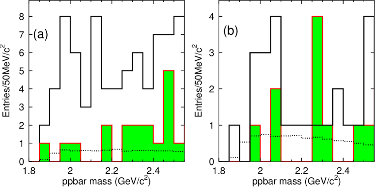
Figure 7: $p\overline{p}$ invariant mass distributions of selected (a) $p\overline{p}\pi^{0}$ and (b) $p\overline{p}\eta$ events. The blank histograms are selected signal events, and the shaded histograms are events from $\pi^{0}$ or $\eta$ mass sidebands. The dashed histograms are predictions of phase space with S-wave $p\overline{p}$ (not normalized).

Fig. 8 shows projections of Dalitz plots in $p\pi$ (or $p\eta$) invariant mass after removing $\psi^{\prime}\rightarrow J/\psi+X$ backgrounds and the possible $p\overline{p}$ mass threshold enhancements. There is a faint accumulation of events in the $p\pi$ invariant mass spectrum at around 2065 MeV/$c^{2}$, but it is not statistically significant. The enhancement between 1.4 and 1.7 GeV/$c^{2}$ may come from $N^{*}(1440)$, $N^{*}(1520)$, $N^{*}(1535)$, etc. We do not attempt a partial wave analysis due to the limited statistics. There is a clear enhancement with $p\eta$ mass at $(1549\pm 13)$ MeV/$c^{2}$, which is possibly the $N^{*}(1535)$.

Figure 8: Projections of Dalitz plots in $p\pi(p\eta)$ invariant mass after removing $\psi^{\prime}\rightarrow\eta J/\psi$ and the possible $R(2000)$. (a) and (b) are $m_{p\pi^{0}}$ and $m_{\overline{p}\pi^{0}}$ in $\psi^{\prime}\rightarrow p\overline{p}\pi^{0}$; (c) is the sum of (a) and (b); (d) and (e) are $m_{p\eta}$ and $m_{\overline{p}\eta}$ in $\psi^{\prime}\rightarrow p\overline{p}\eta$; (f) is the sum of (d) and (e).

VIII Summary

$p\overline{p}\pi^{0}$ and $p\overline{p}\eta$ signals are observed in $\psi^{\prime}$ decays, and the corresponding branching fractions are determined. For $\psi^{\prime}\rightarrow p\overline{p}\pi^{0}$, the errors are much smaller than those of the previous measurement by Mark-II markii , and for $\psi^{\prime}\rightarrow p\overline{p}\eta$, it is the first observation. There is no clear $N^{*}(2065)$ peak in the $p\overline{p}\pi^{0}$ mode, but there is some weak evidence for $p\overline{p}$ threshold enhancements in both channels.

References

(1) J. L. Rosner, Phys. Rev. D 64, 094002 (2001).
(2) P. Wang, C. Z. Yuan and X. H. Mo, Phys. Rev. D
70, 114014 (2004).
(3) N. Isgur, G. Karl, Phys. Rev. D 18, 4187 (1978).
(4) N. Isgur, G. Karl, Phys. Rev. D 19, 2653 (1979).
(5) K. F. Liu, C. W.Wong, Phys. Rev. D 28, 170 (1983).
(6) S. Capstick, N. Isgur, Phys. Rev. D 34, 2809 (1983).
(7) Particle Data Group, S. Eidelman et al.,
Phys. Lett. B 592, 1 (2004).
(8) B. S. Zou, Nucl. Phys. A 675, 167C (2000).
(9) BES Collaboration, J. Z. Bai et al.,
Phys. Lett. B 510, 75 (2001).
(10) BES Collaboration, M. Ablikim et al., hep-ex/0405030.
(11) S. Capstick and W. Roberts, Phys. Rev. D 47, 1994 (1993).
(12) S. Capstick and W. Roberts, Prog. Part. Nucl. Phys.
45, S241 (2000).
(13) C. H. Chang and H. R. Pang, hep-ph/0407188.
(14) Mark-II Collaboration, M. E. B. Franklin. et al.,
Phys. Rev. Lett. 51, 963 (1983).
(15) X. H. Mo et al., HEP&NP 28, 455 (2004).
(16) BES Collaboration, J. Z. Bai et al., Nucl. Instr. Meth.
A 344, 319 (1994).
(17) BES Collaboration, J. Z. Bai et al., Nucl. Instr. Meth.
A 458, 627 (2001).
(18) BES Collaboration, M. Ablikim et al.,
physics/0503001.
(19) J. C. Chen et al., Phys. Rev. D
62, 034003 (2000).
(20) S. M. Li et al., HEP&NP 28, 859 (2004).
(21) BES Collaboration, J. Z. Bai et al.,
Phys. Rev. D 69, 092001 (2004).
(22) BES Collaboration, M. Ablikim et al.,
hep-ex/0408047.
(23) BES Collaboration, J. Z. Bai et al.,
Phys. Rev. D 70, 012005 (2004).
(24) BES Collaboration, J. Z. Bai et al.,
Phys. Rev. D 69, 072001 (2004).