Measurement of the Resonance Parameters of the $\chi_{1}(1^{3}P_{1})$ and $\chi_{2}(1^{3}P_{2})$ States of Charmonium formed in Antiproton-Proton Annihilations

Abstract

We have studied the ${}^{3}P_{J}$ ($\chi_{c})$ states of charmonium in formation by antiproton-proton annihilations in experiment E835 at the Fermilab Antiproton Source. We report new measurements of the mass, width, and $B(\chi_{cJ}\rightarrow\bar{p}p)\times\Gamma(\chi_{cJ}\rightarrow J/\psi+~{}anything)$ for the $\chi_{c1}$ and $\chi_{c2}$ by means of the inclusive reaction $\bar{p}p~{}\rightarrow~{}\chi_{cJ}~{}\rightarrow~{}J/\psi~{}+~{}anything\rightarrow(e^{+}e^{-})+anything$. Using the subsample of events where $\chi_{cJ}\rightarrow\gamma+J/\psi\rightarrow\gamma+(e^{+}e^{-})$ is fully reconstructed, we derive $B(\chi_{cJ}\rightarrow\bar{p}p)\times\Gamma(\chi_{cJ}\rightarrow J/\psi+\gamma)$. We summarize the results of the E760 (updated) and E835 measurements of mass, width and $B(\chi_{cJ}\rightarrow\bar{p}p)\Gamma(\chi_{cJ}\rightarrow J/\psi+\gamma)$ (J=0,1,2) and discuss the significance of these measurements.

I Introduction

Since the discovery of charmonium, it has been clear that the properties of the ${}^{3}P_{J}$ ($\chi_{cJ}$) states are key elements in the understanding of the role and limitations of perturbative Quantum Chromodynamics (pQCD) in this energy regime. The existence of a triplet of P states, split by spin-orbit and tensor force terms, allows us to probe the spin structure of QCD forces.

The production and decay mechanisms of the $\chi_{cJ}$ states are still actively being studied at low energy $e^{+}e^{-}$ storage rings, at high energy colliders and in fixed target experimentsBrambilla . The most precise determinations of mass and width come, however, from our study of charmonium spectroscopy by formation of $\bar{c}c$ states in $\bar{p}p$ annihilation at the Fermilab Antiproton Source (experiments E760 and E835). The E760 collaboration measured the resonance parameters of the $\chi_{c1}$ and $\chi_{c2}$chi12 and more recently we reported measurements of the $\chi_{c0}$ chi0 . In this paper we present the results of new measurements of the $\chi_{c1}$ parameters made, with greatly improved statistics, by E835. The $\chi_{c2}$ parameters were also remeasured with statistics comparable to those of experiment E760. Our E760 results have been updated to account for revised values of reference parameters and are quoted below.

II Experimental technique

We briefly review the technique used in this experiment. A localized source (0.5$\times$0.5$\times$0.6 cm³) of $\bar{p}p$ interactions at instantaneous luminosities up to $5\times 10^{31}$cm^-2s^-1 was obtained by intersecting the beam of stochastically cooled antiprotons circulating in the Accumulator, with a jet of clusterized hydrogen molecules ($\rho_{max}=3.0\times 10^{14}$atoms$/$cm${}^{3})$. The momentum of the antiproton beam was changed in small steps allowing a fine scan of narrow resonances. The parameters of a $\bar{c}c$ resonance (R), mass, width and $B_{R\rightarrow\bar{p}p}\times\Gamma_{R\rightarrow final~{}state}$, were then determined from the excitation curve obtained by measuring the cross section at each value of the antiproton-proton center-of-mass energy ($\sqrt{s}$). With this technique, the systematic uncertainties in the mass and width measurements are greatly reduced since they depend only on the knowledge of the center-of-mass energy.

We determine the center-of-mass energy distribution by measuring the beam-revolution-frequency spectrum and the orbit length, as described in detail in reference psipaper . We calibrate the central orbit length $L_{0}$ using the recent high-precision measurement of the $\psi^{\prime}$ mass by the KEDR experiment, $3686.111\pm 0.025\pm 0.009$ MeV/c² kedr , which gives an uncertainty of $\pm 0.17$ mm out of 474.046 m. $\Delta L$, the correction to $L_{0}$ due to deviations from the central orbit, is determined using 48 horizontal beam-position monitors (BPMs) bigpaper psipaper . For scan I at the $\chi_{c1}$, the uncertainty in $\Delta L$ was estimated as 1 mm (rms) [110 keV] psipaper . The BPM system was subsequently improved and we estimate the uncertainty for the subsequent scans as 0.64 mm (rms) [70 keV at the $\chi_{c1}$, 75 keV at the $\chi_{c2}$]. The center-of-mass energy spread, $\sigma_{\sqrt{s}}$, was approximately 200 keV at the $\chi_{c}$ formation energies.

The cross section for formation of the $\chi_{c}$ states is less than 10^-5 of the inelastic $\bar{p}p$ hadronic cross section. Even so, a clean signal was extracted by selecting electromagnetic final states as tags of charmonium formation. The $\chi_{cJ}$ were studied in the inclusive reaction:

$$\bar{p}p~{}\rightarrow~{}\chi_{cJ}~{}\rightarrow~{}J/\psi+anything\rightarrow~{}(e^{+}e^{-})+anything\,.{}$$ (1)

The non-magnetic spectrometer (Fig.1) was optimized for the detection of photons and electrons, and is described in detail in reference bigpaper . The apparatus had full acceptance in azimuth ($\phi$), with a cylindrical central system and a planar forward system. The detector elements used for the trigger and for the offline selection of events from reaction (1) were (a) three hodoscopes, $H1$, $H2^{\prime}$ and $H2$, azimuthally segmented in 8, 24 and 32 counters respectively, (b) a threshold gas Čerenkov counter for identifying $e^{\pm}$, divided in two volumes in polar angle; each volume was segmented azimuthally in 8 sectors aligned with the counters of the $H1$ hodoscope, and (c) two lead-glass calorimeters for measuring the energy and direction of photons and electrons: a cylindrical one (CCAL) with 1280 counters, covering the polar angles $11^{\circ}<\theta<70^{\circ}$ and a planar one (FCAL) covering the polar angles $3^{\circ}<\theta<12^{\circ}$. All counters were equipped with time and pulse-height measurement capability. The luminosity was measured at each data point with a statistical precision of $0.1\%$ and systematic uncertainty of $\pm 2.5\%$, by counting recoil protons from elastic $\bar{p}p$ scattering in three solid state detectors located at $87.5^{\circ}$ to the beam direction.

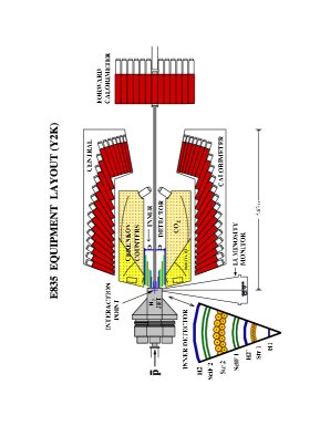
Figure 1: The E835 detector, side view

The hardware trigger was designed to select events with a $J/\psi\rightarrow e^{+}e^{-}$ decay in the central detector charge . It required two charged tracks, each defined by a coincidence between two hodoscope counters ($H1\times H2$) aligned in azimuth, with at least one of the two particles tagged as an electron by a signal in the corresponding Čerenkov cell. In addition, two large energy deposits (clusters) separated by more than 90^∘ in azimuth and with an invariant mass greater than 60$\%$ of the center of mass energy, were required in the CCAL. The efficiency of this trigger was measured to be $0.90\pm 0.02$ from a clean sample of $\bar{p}p\rightarrow\psi^{\prime}\rightarrow e^{+}e^{-}$ events, taken with relaxed trigger conditions. Online, a filtering program certified as electron candidates CCAL energy clusters aligned with tracks formed by the hodoscopes and Čerenkov elements.

III Data analysis

The data presented here were collected by experiment E835, in three scans performed at the $\chi_{c1}$ in August 1997 (scan I), February 2000 (scan II), and July 2000 (scan III), and one scan performed at the $\chi_{c2}$ in February 2000. The center of mass energy, $\sqrt{s}$, width of the $\sqrt{s}$ distribution, $FWHM_{\sqrt{s}}$, and integrated luminosity, ${\it Ldt}$, for each $run$ are given in Table 1.

Our data analysis methods are described in detail in reference bigpaper . The offline selection of $\chi_{c1}$ and $\chi_{c2}$ events compatible with reaction (1) is done in three steps; the first two are illustrated in Fig. 2 which shows, at each step, the invariant mass distribution of the $e^{+}~{}e^{-}$ candidates for on-resonance data and (shaded) for data taken off-resonance, normalized to the integrated luminosity of the data taken in the resonance region. In the first step (Fig. 2a), all events with two electron (i.e. electron-positron) candidates within the Čerenkov fiducial region ($15^{\circ}<\theta<60^{\circ}$) and an invariant mass ($M_{ee}$) above 2600 MeV/c² are selected. A clear enhancement is seen in the on-resonance data at the mass of the $J/\psi$. In the next step, the electron candidates are identified by using an “electron weight” parameter, which is a likelihood ratio for the electron hypothesis versus the background hypothesis. It uses the pulse heights in the three hodoscopes ($H1$,$H2^{\prime}$,$H2$) and Čerenkov counter, and the transverse energy distribution of the CCAL clusters, and distinguishes single electron tracks from background (predominantly $e^{+}e^{-}$ pairs from photon conversions in the 0.18 mm thick steel beam-pipe and $\pi^{0}\rightarrow e^{+}e^{-}\gamma$ decays). The resulting $e^{+}e^{-}$ invariant mass distribution is shown in Fig. 2b. The slight enhancement in the background level at the $J/\psi$ mass peak comes from the continuum of $\bar{p}p\rightarrow\pi^{0}J/\psi$ events.

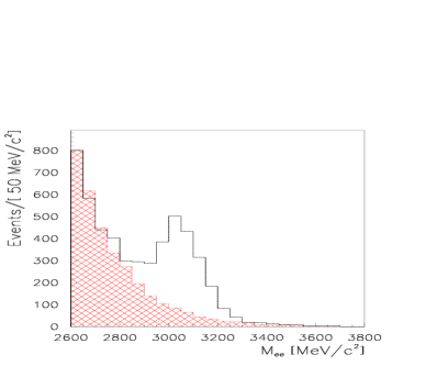
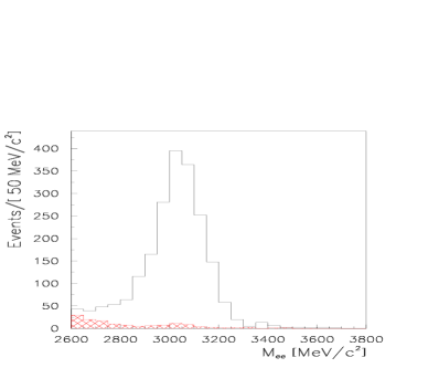
Figure 2: Reconstructed e⁺e^- invariant-mass distribution for events in the $\chi_{c1}$ resonance region(clear), and for events off-resonance(shaded): (a) all events with both electron candidates within the Čerenkov fiducial volume, (b) events remaining after applying the electron-weight cut.

We select $J/\psi X$ events by applying a 1C kinematical fit to the reaction: $\bar{p}p\rightarrow\chi_{cJ}\rightarrow J/\psi+anything\rightarrow(e^{+}e^{-})+anything$, accepting events with $\chi^{2}$ probability greater than $10^{-2}$ and with $M_{ee}>2800$ MeV/c². The number $N(J/\psi X)$ of events selected for each run is given in Table 1. The efficiency for event selection is determined from a sample of events collected in a run (labeled efficiency in Table 1) taken near the $\chi_{c1}$ resonance peak energy, and is 0.865 $\pm$ 0.015. The geometrical acceptances are calculated by Monte Carlo simulation, fixing the parameters of the angular distributions of reaction (1) to values measured previously angdis . The acceptances are $0.610\pm 0.006$ for the $\chi_{c1}$ and $0.617\pm 0.006$ for the $\chi_{c2}$, where the errors include uncertainties in the acceptance-volume boundaries and angular-distribution parameters. After including trigger and selection efficiencies, we obtain the overall efficiencies ($\epsilon$) given in Table 2.

We select $J/\psi\gamma$ events from the inclusive sample by requiring one additional on-time cluster within the fiducial volumes of CCAL (12${}^{\circ}<\theta<$68^∘) or FCAL (3${}^{\circ}<\theta<$10^∘). [For scan I at the $\chi_{c1}$ we did not use FCAL.] A 5C kinematic fit to the reaction:

$$\bar{p}p\rightarrow J/\psi+\gamma\rightarrow(e^{+}e^{-})+\gamma{}$$ (2)

is applied and events with $\chi^{2}$ probability less than $10^{-3}$ are rejected. The number $N(J/\psi\gamma)$ of events selected for each run is given in Table 1. The geometrical acceptances are $0.498\pm 0.01$ for the $\chi_{c1}$ [$0.456\pm 0.01$ for scan I] and $0.519\pm 0.01$ for the $\chi_{c2}$. The overall efficiencies ($\epsilon$) are given in Table 2.

	$\sqrt{s}$	$FWHM_{\sqrt{s}}$	Ldt	N($J/\psi$ X)	N$(J/\psi\gamma)$
	[MeV]	[keV]	[nb-1]
	3513.00	713	301.3	24	14
$\chi_{1}$	3511.44	740	315.5	110	77
scan I	3511.05	723	319.4	178	120
Aug. 97	3510.75	682	318.8	266	175
	3510.36	656	315.0	217	151
	3509.93	592	317.1	101	66
	3508.59	545	376.2	20	11
	3494.43	788	502.8	10	2
	3524.64	717	3716.9	57	14
	3525.16	661	2903.0	53	20
	3511.79	635	184.9	36	27
	3511.39	566	200.9	84	62
$\chi_{1}$	3511.03	562	190.8	139	101
scan II	3510.56	550	199.5	182	129
Feb. 00	3510.15	512	235.3	122	83
	3509.74	457	319.0	67	48
	3511.69	727	452.1	77	47
$\chi_{1}$	3510.69	675	417.6	338	241
scan III	3511.17	746	441.0	214	147
July 00	3510.21	604	493.4	333	245
	3509.69	472	750.2	186	140
efficiency	3510.62	721	1874.2	1422	1049
	3558.80	533	144.4	20	19
	3557.31	519	205.5	86	70
$\chi_{2}$	3555.82	481	267.0	248	191
Feb. 00	3554.29	439	225.4	54	49
	3535.10	444	211.0	5	1
	3469.90	802	2512.6	20	2
background	3525.17	708	3709.6	44	11
00	3523.33	920	3058.6	49	17
	3524.79	701	2033.0	33	13

Table 1: Center of mass energy ($\sqrt{s}$) and width of $\sqrt{s}$ distribution ($FWHM_{\sqrt{s}}$), integrated luminosity Ldt, and number of events selected (N) for the inclusive ($J/\psi X$) and exclusive ($J/\psi\gamma$) decay channels for each data run used in this analysis.

Scan I, performed in 1997, includes three background points distant from the $\chi_{c1}$. The entries labeled background in Table 1 refer to data taken in 2000 that are far from the $\chi_{c}$ resonances. The background point at $\sqrt{s}$ = 3469.9 MeV is used only for the $\chi_{c1}$ analysis while the other three points are used for both $\chi_{c1}$ and $\chi_{c2}$.

	$\chi_{c1}$ Scan I
	$\bar{p}p\rightarrow\chi_{c1}\rightarrow J/\psi+X$	$\bar{p}p\rightarrow\chi_{c1}\rightarrow J/\psi+\gamma$
	$J/\psi\rightarrow e^{+}e^{-}$	$J/\psi\rightarrow e^{+}e^{-}$
$M_{\chi_{c1}}$ [MeV/c2]	$3510.749\pm 0.122$	$3510.749\pm 0.113$
$\Gamma_{\chi_{c1}}$ [MeV]	$0.89\pm 0.09$	$0.89\pm 0.09$
B${}_{in}\times\Gamma_{out}$[eV]	$1.25\pm 0.06$	$1.20\pm 0.06$
$\sigma_{b}$[pb]	$14.5\pm 1.6$	$3.4\pm 0.9$
$\epsilon$	$0.459\pm 0.011$	$0.328\pm 0.010$
$\chi^{2}$/D.F.	7.2/6	11.5/14
	$\chi_{c1}$ Scan II
	$\bar{p}p\rightarrow\chi_{c1}\rightarrow J/\psi+X$	$\bar{p}p\rightarrow\chi_{c1}\rightarrow J/\psi+\gamma$
	$J/\psi\rightarrow e^{+}e^{-}$	$J/\psi\rightarrow e^{+}e^{-}$
$M_{\chi_{c1}}$ [MeV/c2]	$3510.783\pm 0.075$	$3510.784\pm 0.075$
$\Gamma_{\chi_{c1}}$ [MeV]	$0.87\pm 0.08$	$0.88\pm 0.09$
B${}_{in}\times\Gamma_{out}$[eV]	$1.33\pm 0.06$	$1.22\pm 0.06$
$\sigma_{b}$[pb]	$10.4\pm 1.1$	$2.2\pm 0.6$
$\epsilon$	$0.475\pm 0.015$	$0.382\pm 0.014$
$\chi^{2}$/D.F.	5.6/6	12.3/14
	$\chi_{c1}$ Scan III
	$\bar{p}p\rightarrow\chi_{c1}\rightarrow J/\psi+X$	$\bar{p}p\rightarrow\chi_{c1}\rightarrow J/\psi+\gamma$
	$J/\psi\rightarrow e^{+}e^{-}$	$J/\psi\rightarrow e^{+}e^{-}$
$M_{\chi_{c1}}$ [MeV/c2]	$3510.643\pm 0.074$	$3510.641\pm 0.074$
$\Gamma_{\chi_{c1}}$ [MeV]	$0.87\pm 0.06$	0.$88\pm 0.07$
B${}_{in}\times\Gamma_{out}$[eV]	$1.25\pm 0.04$	$1.14\pm 0.04$
$\sigma_{b}$[pb]	$10.5\pm 1.1$	$2.3\pm 0.6$
$\epsilon$	$0.475\pm 0.015$	$0.382\pm 0.014$
$\chi^{2}$/D.F.	6.4/5	17.3/12
	$\chi_{c2}$
	$\bar{p}p\rightarrow\chi_{c2}\rightarrow J/\psi+X$	$\bar{p}p\rightarrow\chi_{c2}\rightarrow J/\psi+\gamma$
	$J/\psi\rightarrow e^{+}e^{-}$	$J/\psi\rightarrow e^{+}e^{-}$
$M_{\chi_{c2}}$ [MeV/c2]	$3556.173\pm 0.123$	$3556.168\pm 0.114$
$\Gamma_{\chi_{c2}}$ [MeV]	$1.92\pm 0.19$	$1.95\pm 0.19$
B${}_{in}\times\Gamma_{out}$[eV]	$1.60\pm 0.09$	$1.59\pm 0.10$
$\sigma_{b}$[pb]	$12.0\pm 1.3$	$2.6\pm 0.7$
$\epsilon$	$0.481\pm 0.017$	$0.398\pm 0.014$
$\chi^{2}$/D.F.	3.6/4	18.9/10

Table 2: Fit results for $\chi_{c1}$ and $\chi_{c2}$ parameters, listed separately by scan. The $J/\psi X$ results are obtained by fitting the inclusive sample. The $J/\psi\gamma$ results are obtained from a joint fit to the $J/\psi\gamma$ sample and the remaining $J/\psi X$ events (see text). The errors include fitting uncertainties and random uncertainties in the beam-orbit length.

The cross section: $\sigma_{meas}(\sqrt{s_{i}})=\frac{N_{i}}{{\it L_{i}}\times\epsilon}$, measured at the $i$th point of a scan, is given by:

$$\sigma_{meas}(\sqrt{s_{i}})=\sigma_{b}+\int~{}[f_{i}(\sqrt{s_{i}}-\sqrt{s^{\prime}})\times~{}\sigma_{BW}^{rad}(\sqrt{s^{\prime}})]~{}d\sqrt{s^{\prime}}\,~{}~{}~{}~{}~{}~{}~{}~{}~{}~{}{}$$ (3)

where $\sigma_{b}$ is the background cross section, which we take to be constant over each scan, $f_{i}(\sqrt{s_{i}}-\sqrt{s^{\prime}})$ is the normalized $\sqrt{s}$ distribution at the ith point and $\sigma_{BW}^{rad}$ is the Breit-Wigner resonance cross section corrected for initial state radiation (see appendix A). The Breit-Wigner cross section is:

$$\sigma_{BW}(\sqrt{s})=\frac{\pi(2J+1)}{k^{2}}\times\frac{\Gamma_{\chi_{cJ}}\times B_{in}\times\Gamma_{out}}{4(\sqrt{s}-M_{\chi_{cJ}})^{2}+\Gamma_{\chi_{cJ}}^{2}}~{}~{}~{}~{}{}$$ (4)

where $k^{2}=\frac{s-4m_{p}^{2}}{4}$, $m_{p}$ is the proton mass, $J$, $M_{\chi_{cJ}}$ and $\Gamma_{\chi_{cJ}}$ are the spin, mass and width of the $\chi_{cJ}$ resonance, $B_{in}=B(\chi_{cJ}\rightarrow\bar{p}p)$ and $\Gamma_{out}=\Gamma(\chi_{cJ}\rightarrow J/\psi+~{}anything~{})\times B(J/\psi\rightarrow e^{+}e^{-}$).

A maximum likelihood fit to equation (3) is performed to find the values of $M_{\chi_{cJ}}$, $\Gamma_{\chi_{cJ}}$, $\sigma_{b}$, and $B_{in}\times\Gamma_{out}$. This last parameter effectively measures the area of the Breit-Wigner since $B_{in}\times\Gamma_{out}$ can be rewritten as $(B_{in}B_{out})\times\Gamma_{\chi_{cJ}}$ and ($B_{in}B_{out}$) measures the cross section at the peak of the resonance. The errors in $M_{\chi_{cJ}}$ are the in-quadrature sums of uncertainties from the maximum-likelihood fits and uncertainties in corrections to the beam-orbit length, which is used in the determination of the center-of-mass energy as described above. To determine the value of $B_{in}\times\Gamma(\chi_{c1}\rightarrow J/\psi+\gamma)\times B(J/\psi\rightarrow e^{+}e^{-})$ we perform a joint maximum likelihood fit to equation (3) of the two independent samples of events: 1. $J/\psi\gamma$ fits, and 2. $J/\psi X$ events not fitting $J/\psi\gamma$ (see Table 1), constraining $M_{\chi_{c1}}$ and $\Gamma_{\chi_{c1}}$ to be the same for the two samples and allowing $\sigma_{b}$ and $B_{in}\Gamma_{out}$ to be different. The results of the fits are given in Table 2.

In Fig. 3a we plot, at each point of scan III at the $\chi_{c1}$ plus background points, the measured cross section ($\sigma_{meas}$) superimposed on the excitation curve obtained from the fitted parameters listed in Table 2, column 3. The same graphical representation of the results of the $\chi_{c2}$ scan is given in Fig. 3b. To illustrate the effect of scanning a narrow resonance with a beam of comparable width, we show in Fig. 4a a blow up of scan II at the $\chi_{c1}$, where the horizontal errors are the $FWHM_{\sqrt{s}}$. The solid curve is the fit to Eq. 3, and includes the spread in $\sqrt{s}$. The dashed curve is the sum of $\sigma_{b}$ and the Breit-Wigner cross section $\sigma_{BW}(\sqrt{s})$ given by Eq. (4). The parameters for the curves are given in Table 2, column 2.

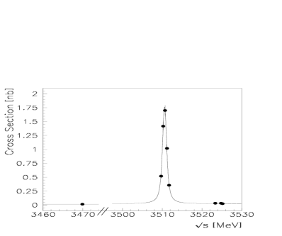
Figure 3: (a)The measured cross sections and fitted excitation curve for scan III of the $\chi_{c1}$ plus background points. (b) The measured cross sections and excitation curve for the $\chi_{c2}$ scan plus background points.

Figure 4: (a)The measured cross section for scan II at the $\chi_{c1}$. The horizontal errors are the $FWHM_{\sqrt{s}}$ . The solid curve is the fit to Eq. 3, and includes the spread in $\sqrt{s}$. The dashed curve is the sum of $\sigma_{b}$ and the Breit-Wigner cross section $\sigma_{BW}(\sqrt{s})$ given by Eq. (4). (b)The $\sqrt{s}$ distribution for each point of the scan.

IV Results

The results from the individual $\chi_{c1}$ scans are in good agreement and therefore we take for each parameter the weighted (by the inverse variance) average of the measurements. The resulting values of the parameters for the two methods of determining them are given in Table 3, along with the corresponding $\chi_{c2}$ results. The errors shown are (i) statistical, (ii) from uncertainties in auxiliary variables, which were measured during data taking, and (iii) from uncertainties in external parameters measured in other experiments. The last of these uncertainties may eventually be reduced. The auxiliary-variable error in $\Gamma_{\chi_{cJ}}$ comes from uncertainty in $\eta$, the slip factor relating frequency and momentum excursions in the storage ring psipaper , mcginnis , which is used to determine the $FWHM_{\sqrt{s}}$. That in $B_{in}\Gamma_{out}$ is estimated by adding in quadrature the errors in detector and luminosity-monitor acceptance and efficiency. The external-parameter error in $M_{\chi_{cJ}}$ comes from the uncertainty in the $\psi^{\prime}$ mass used in the absolute calibration of the beam energy psipaper as described above. For $B_{\bar{p}p}\Gamma_{J/\psi X}$ and $B_{\bar{p}p}\Gamma_{J/\psi\gamma}$, the uncertainties in the parameters of the elastic scattering cross section elastic , which are the limiting errors in the estimate of luminosity, the parameters of the final state angular distributions angdis , and the branching ratio $B_{J/\psi\rightarrow e^{+}e^{-}}$, where we use $0.0593\pm 0.001$, are added in quadrature. The error contributions are summarized in Table 4.

	$\bar{p}p\rightarrow\chi_{c1}\rightarrow J/\psi+X$	$\bar{p}p\rightarrow\chi_{c1}\rightarrow J/\psi+\gamma$
$M_{\chi_{c1}}$ [MeV/c2]	$3510.719\pm 0.051\pm 0.019_{ext}$	$3510.713\pm 0.051\pm 0.019_{ext}$
$\Gamma_{\chi_{c1}}$ [MeV]	$0.876\pm 0.045\pm 0.026_{aux}$	$0.881\pm 0.052\pm 0.026_{aux}$
B${}_{\bar{p}p}\times\Gamma_{out}$ [eV]	$21.5\pm 0.5\pm 0.6_{aux}\pm 0.6_{ext}$	$19.8\pm 0.5\pm 0.6_{aux}\pm 0.6_{ext}$
$\sigma_{b}$[pb]	$10.5\pm 1.0$	$2.5\pm 0.4$
	$\bar{p}p\rightarrow\chi_{c2}\rightarrow J/\psi+X$	$\bar{p}p\rightarrow\chi_{c2}\rightarrow J/\psi+\gamma$
$M_{\chi_{c2}}$ [MeV/c2]	$3556.173\pm 0.123\pm 0.020_{ext}$	$3556.168\pm 0.114\pm 0.020_{ext}$
$\Gamma_{\chi_{c2}}$ [MeV]	$1.915\pm 0.188\pm 0.013_{aux}$	$1.953\pm 0.187\pm 0.013_{aux}$
B${}_{\bar{p}p}\times\Gamma_{out}$ [eV]	$27.0\pm 1.5\pm 0.8_{aux}\pm 0.7_{ext}$	$26.8\pm 1.7\pm 0.8_{aux}\pm 0.8_{ext}$
$\sigma_{b}$[pb]	$12.0\pm 1.3$	$2.6\pm 0.7$

Table 3: E835 results for $\chi_{c1}$ and $\chi_{c2}$ resonance parameters for the J/$\psi+X$ and J/$\psi+\gamma$ final states. The first errors are statistical; the second and third are auxiliary-variable and external-parameter systematic errors given in Table 4.

Resonance Parameters		Auxiliary Variables
	$\eta$	Effic.	Lumin.	Total
$\Gamma_{\chi_{c1}}$	26 keV	-	-	26 keV
$\Gamma_{\chi_{c2}}$	13 keV	-	-	13 keV
$B_{\bar{p}p}\Gamma(\chi_{cJ}\rightarrow J/\psi\gamma)$	-	3.0$\%$	0.6$\%$	3.1$\%$
$B_{\bar{p}p}\Gamma(\chi_{cJ}\rightarrow J/\psi$ X )	-	2.8$\%$	0.6$\%$	2.9$\%$

Resonance Parameters		External Parameters
	M${}_{\psi^{\prime}}$	a2,B0	$\sigma_{tot},b,\rho$	$B(J/\psi\rightarrow e^{+}e^{-})$	Total
$M_{\chi_{c1}}$	19 keV/c2	-	-		19 keV/c2
$M_{\chi_{c2}}$	20 keV/c2	-	-		20 keV/c2
$B_{\bar{p}p}\Gamma(\chi_{c1}\rightarrow J/\psi\gamma)$	-	-	2.1$\%$	1.7$\%$	2.7$\%$
$B_{\bar{p}p}\Gamma(\chi_{c2}\rightarrow J/\psi\gamma)$	-	1.3$\%$	2.1$\%$	1.7$\%$	3.0$\%$
$B_{\bar{p}p}\Gamma(\chi_{c1}\rightarrow J/\psi$ X)	-	-	2.1$\%$	1.7$\%$	2.7$\%$
$B_{\bar{p}p}\Gamma(\chi_{c2}\rightarrow J/\psi$ X)	-	0.5$\%$	2.1$\%$	1.7$\%$	2.7$\%$

Table 4: Uncertainties due to errors in auxiliary variables and external parameters. In the top panel we refer to variables measured during data taking, while the bottom panel refers to parameters measured by other experiments: $\eta$ is the slip factor relating frequency and momentum excursions in the storage ring; $a_{2}$ and $B_{0}$ characterize the $\chi_{c}$ decay angular distributions angdis ; $\sigma_{tot}$, $b$, and $\rho$ parametrize the $\bar{p}p$ elastic cross section elastic . Within each category, the contributions are added in quadrature.

In Fig. 5 a) and b) we compare the results of our mass measurements for $\chi_{c1}$ and $\chi_{c2}$ to the values obtained in other experiments in the last twenty years. The comparison clearly shows the advantage of using this technique. For the width measurements, the only results of precision comparable to those of E835 were obtained by our predecessor experiment, E760. These are listed in Table 5.

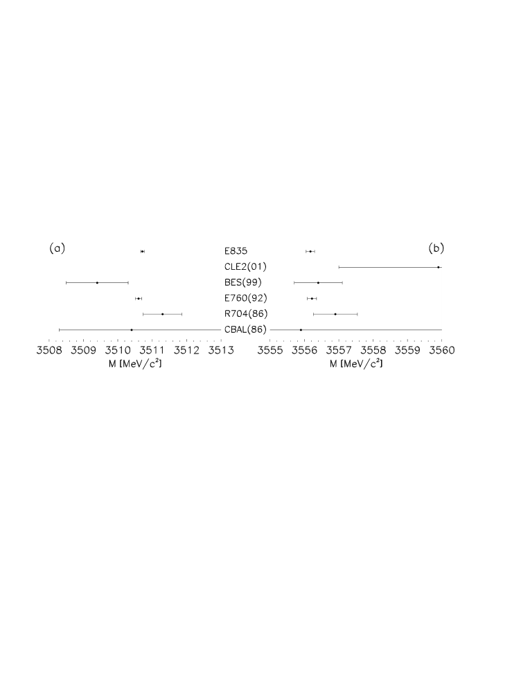
Figure 5: $\chi_{c1}$ (a) and $\chi_{c2}$ (b) masses from this and other experiments. The error bars represent the in-quadrature sums of statistical and systematic errors.

V Discussion

Our experimental study of charmonium is based on three data taking periods in the years 1990-1991 (E760)chi12 , 1996-1997 (Run 1 of E835) and 2000 (Run 2 of E835). Table 5, where we compare E835 with E760, shows good agreement for all measured parameters. In the nine year gap between the first and last data-taking periods, major modifications of the Accumulator lattice and of the beam diagnostic system took place and elements of the target-detector complex were substituted or upgraded. We consider the consistency between the two experiments evidence of our understanding of the related systematic uncertainties.

In Table 5, the values measured by E760 are adjusted as follows: $M_{\chi_{cJ}}$ are adjusted to reflect the KEDR high-precision $\psi^{\prime}$ mass measurement referred to above; $M_{\chi_{cJ}}$, $\Gamma_{\chi_{cJ}}$ and $B_{\bar{p}p}\times\Gamma(\chi_{cJ}\rightarrow J/\psi+\gamma)$ are adjusted by the small shifts induced by fitting to the Breit-Wigner cross section corrected for radiative effects (see Appendix A and Table 8); $B_{\bar{p}p}\times\Gamma(\chi_{cJ}\rightarrow J/\psi+\gamma)$ are corrected for a $6.5\%$ underestimate of the luminosity (Ldt), which we discovered after publication of the results. The orbit uncertainty from the BPM system is included in the statistical error and the systematic error in $M_{\chi_{cJ}}$ comes entirely from the $\psi^{\prime}$ mass uncertainty; the systematic error in $\Gamma_{\chi_{cJ}}$ comes entirely from the uncertainty in $\eta$, and that in $B_{\bar{p}p}\times\Gamma(\chi_{cJ}\rightarrow J/\psi+\gamma)$ has contributions from auxilliary variables and external parameters. For completeness, we include the results from our recent measurement of the resonance parameters of the $\chi_{c0}$ state chi0 . These values are adjusted for the KEDR $\psi^{\prime}$ mass and radiative effects.

Using the E835 values, we derive (Table 6) the fine structure splittings $\Delta M_{21}=M_{\chi_{c2}}-M_{\chi_{c1}}$ and $\Delta M_{10}=M_{\chi_{c1}}-M_{\chi_{c0}}$, the ratio $\rho$ = $\frac{\Delta M_{21}}{\Delta M_{10}}$, and the $\chi_{cJ}$ center of gravity, $M_{c.o.g.}=\frac{M_{\chi_{c0}}+3M_{\chi_{c1}}+5M_{\chi_{c2}}}{9}$. The uncertainties contain the statistical and systematic errors added in quadrature, accounting for systematic errors in common.

	$\chi_{c0}$
PARAMETER	E835
$M_{\chi_{c0}}$ [MeV/c2]	$3415.5\pm 0.4\pm 0.4$
$\Gamma_{\chi_{c0}}$ [MeV]	$9.7\pm 1.0$
$B_{\bar{p}p}\times\Gamma(\chi_{c0}\rightarrow J/\psi+\gamma)$ [eV]	$28.0\pm 1.9\pm 1.3$
	$\chi_{c1}$
PARAMETER	E835	E760
$M_{\chi_{c1}}$ [MeV/c2]	$3510.719\pm 0.051\pm 0.019_{ext}$	$3510.60\pm 0.087\pm 0.019$
$\Gamma_{\chi_{c1}}$ [MeV]	$0.876\pm 0.045\pm 0.026_{aux}$	$0.87\pm 0.11\pm 0.08$
$B_{\bar{p}p}\times\Gamma(\chi_{c1}\rightarrow J/\psi+\gamma)$ [eV]	$21.5\pm 0.5\pm 0.6_{aux}\pm 0.6_{ext}$	$21.4\pm 1.5\pm 2.2$
	$\chi_{c2}$
PARAMETER	E835	E760
$M_{\chi_{c2}}$ [MeV/c2]	$3556.173\pm 0.123\pm 0.020_{ext}$	$3556.22\pm 0.131\pm 0.020$
$\Gamma_{\chi_{c2}}$ [MeV]	$1.915\pm 0.188\pm 0.013_{aux}$	$1.96\pm 0.17\pm 0.07$
$B_{\bar{p}p}\times\Gamma(\chi_{c2}\rightarrow J/\psi+\gamma)$ [eV]	$27.0\pm 1.5\pm 0.8_{aux}\pm 0.7_{ext}$	$27.7\pm 1.5\pm 2.0$

Table 5: Comparison of the values of the $\chi_{c1}$ and $\chi_{c2}$ parameters measured in E835 with those measured by E760. The E835 $\chi_{c0}$ values are included for completenesschi0 . The mass and width values come from the $\bar{p}p\rightarrow J/\psi+X$ fits. The E760 and E835 $\chi_{c0}$ values are referred to the KEDR $\psi^{\prime}$ mass and radiative corrections are made. The E760 values are corrected for the luminosity error described in the text.

$\Delta M_{21}=M_{\chi_{c2}}-M_{\chi_{c1}}$ [MeV/c2]	$45.45\pm 0.15$
$\Delta M_{10}=M_{\chi_{c1}}-M_{\chi_{c0}}$ [MeV/c2]	$95.2\pm 0.6$
$\rho$ = $\frac{\Delta M_{21}}{\Delta M_{10}}$	$0.477\pm 0.002$
$M_{c.o.g.}=\frac{M_{\chi_{c0}}+3M_{\chi_{c1}}+5M_{\chi_{c2}}}{9}$ [MeV/c2]	$3525.39\pm 0.10$

Table 6: Fine-structure splittings ($\Delta M_{ik}$), ratio of fine-structure splittings ($\rho$) and ${}^{3}P_{J}$ states center-of-gravity ($M_{c.o.g.})$, as derived from mass values measured by E835.

In the Breit-Fermi theory, the $\chi_{cJ}$ and $h_{c}$ masses can be written as:

$$M_{J}=M_{0}+\langle h_{LS}\rangle\times\langle\vec{L}.\vec{S}\rangle_{J}+\langle h_{T}\rangle\times\langle S_{12}\rangle_{J}$$ (5)

where the three terms are, respectively, the expectation values of the spin-independent, spin-orbit and tensor components of the $\bar{c}c$ Hamiltonian Lucha . If we assume the $\chi_{c}$ to be pure ($\bar{c}c$) states and their spatial wavefunctions to be identical, M₀ is the same for the three states and the mass splittings yield the values of $\langle h_{LS}\rangle$ and $\langle h_{T}\rangle$. As

$$\langle\vec{L}.\vec{S}\rangle_{J}=-2,-1,1$$

and

$$\langle S_{12}\rangle_{J}=12(\frac{(\vec{S}_{1}.\vec{r})(\vec{S}_{2}.\vec{r})}{r^{2}}-\frac{\vec{S}_{1}.\vec{S}_{2}}{3})=-4,2,-\frac{2}{5}$$

for J = 0,1,2 respectively, we obtain the spin-orbit contribution:

$$\langle h_{LS}\rangle=\frac{2\Delta M_{10}+5\Delta M_{21}}{12}=34.80\pm 0.09~{}{\rm MeV/c}^{2}$$ (6)

and the tensor contribution:

$$\langle h_{T}\rangle=\frac{10\Delta M_{10}-5\Delta M_{21}}{72}=10.06\pm 0.06~{}{\rm MeV/c}^{2}.$$ (7)

Assuming (as above) that the spatial wave functions of the $\chi_{cJ}$ states are identical, the partial widths for the E1 transitions $\chi_{cJ}\rightarrow J/\psi\gamma$ are expected to scale as $E_{\gamma}^{3}$. Our recent measurement of $\Gamma_{\chi_{c0}}$ chi0 and improved measurements of $B(\chi_{c0}\rightarrow J/\psi\gamma)$ pdg04 allow us to test this prediction for all three $\chi_{J}$. We have performed a fit to the $\psi^{\prime}$ and $\chi_{cJ}$ branching ratios analogous to that described in Reference pdg04 to obtain the radiative widths, which are given in Table 7. These are in agreement with $E_{\gamma}^{3}$ scaling.

	$\chi_{c0}$	$\chi_{c1}$	$\chi_{c2}$
$E_{\gamma}$ [MeV]	304	389	430
$\Gamma(\chi_{cJ}\rightarrow J/\psi\gamma)$ [keV]	$119\pm 16$	$280\pm 32$	$416\pm 34$
$\Gamma(\chi_{cJ}\rightarrow J/\psi\gamma)/E_{\gamma}^{3}$ [$10^{-9}$MeV-2]	$4.12\pm 0.57$	$4.74\pm 0.54$	$5.24\pm 0.43$

Table 7: Partial widths for the E1 transitions $\chi_{cJ}\rightarrow J/\psi\gamma$ showing agreement with $E_{\gamma}^{3}$ scaling. These values are obtained from a global fit to the data tabulated in Reference pdg04 and our results.

VI Summary

Fermilab experiment E835 and our earlier experiment, E760, have measured the resonance parameters and $B(\bar{c}c\rightarrow\bar{p}p)\times\Gamma(\bar{c}c\rightarrow$ final state) for charmonium states formed in antiproton-proton annihilations. We have directly determined the masses and widths of these states with unprecendented precision in extremely low-background conditions.

In this paper we compile the resonance parameters of the ${}^{3}P_{J}$ states. We report new measurements of $\chi_{c1}$ and $\chi_{c2}$ detected through the decay channels $J/\psi+anything$ and $J/\psi+\gamma$, and find excellent agreement between these results and those obtained by experiment E760. From the mass measurements we derive the fine-structure splittings between $\chi_{c0}$, $\chi_{c1}$, and $\chi_{c2}$ with a precision of a fraction of a percent. We find that the radiative widths for the $E1$ transitions $\chi_{cJ}\rightarrow J/\psi\gamma$ scale as $E_{\gamma}^{3}$ as expected.

VII Acknowledgments

We gratefully acknowledge the support of the Fermilab staff and technicians and especially the Antiproton Source Department of the Accelerator Division and the On-Line Department of the Computing Division. We wish to thank also the INFN and university technicians and engineers from Ferrara, Genova, Torino and Northwestern for the valuable work done. This research was supported by the Italian Istituto Nazionale di Fisica Nucleare (INFN) and U.S. Department of Energy.

VIII Appendix A

In the analysis of an excitation profile the Breit-Wigner resonance cross section must be corrected to account for the radiation of the incoming particle in the electromagnetic field of the target particle. For a $\bar{p}p$ initial state, D. C. Kennedy kennedy has derived the following expression for the corrected Breit-Wigner cross-section:

$$\sigma_{BW}^{rad}(\beta,s)=\beta\int_{0}^{\sqrt{s}\over 2}{dk\over k}({2k\over\sqrt{s}})^{\beta}\sigma_{BW}(s-2k\sqrt{s})$$ (8)

with

$$\beta=\frac{2\alpha}{\pi}\times[\frac{s-2m_{p}^{2}}{\sqrt{s\times(s-4m_{p}^{2})}}\times ln(\frac{s+\sqrt{s\times(s-4m_{p}^{2})}}{s-\sqrt{s\times(s-4m_{p}^{2})}})-1].$$ (9)

In our analysis we have convolved the corrected Breit-Wigner cross section with the beam distribution at each point in the scan; in this way we properly account for the conditions of data taking. As the radiated photon energy falls between zero and half the total energy, and we wish to correct $\Gamma_{R}$ at the one-percent level, which means 0.01/3500=3$\times$ 10^-6 of the total energy, particular care was taken to avoid rounding errors in performing the numerical integration. In Table 8 we list, for the three $\chi_{c}$ states, the change in the measured parameters resulting from the application of radiative corrections. These changes are significantly smaller than the uncertainties in the measurements.

	$\chi_{c0}$	$\chi_{c1}$	$\chi_{c2}$
$M_{\chi_{cJ}}$ [MeV/c2]	-0.06	- 0.01	-0.02
$\Gamma_{\chi_{cJ}}$	-1.2 $\%$	-1.1 $\%$	-0.9 $\%$
$B_{\bar{p}p}\times\Gamma(\chi_{cJ}\rightarrow J/\psi+\gamma)$	+3.2 $\%$	+5.0 $\%$	+4.5 $\%$

Table 8: Shifts in the values of the resonance parameters when radiative corrections are applied

References

• (1) N.Β Brambilla et al., arXiv:hep-ph/0412158 and references therein (2004)
• (2) E760 Collaboration, T.A.Armstrong et al., Nucl. Phys. B373, 35 (1992)
• (3) E835 Collaboration, S. Bagnasco et al., Phys. Lett. B533, 234 (2002)
• (4) E835 Collaboration, G. Garzoglio et al., Nuc. Inst. Meth. A519, 558 (2004)
• (5) Our detector did not determine the sign of the particle charge; we assume the charges of the two electrons in these events to be opposite.
• (6) E835 Collaboration, M. Ambrogiani et al., Phys. Rev. D65, 052002 (2002)
• (7) E760 Collaboration, T.A.Armstrong et al., Phys. Rev. D47, 772 (1993)
• (8) D. P. McGinnis, G. Stancari, S. J. Werkema, Nuc. Inst. Meth. A506, 205 (2003)
• (9) KEDR Collaboration, V.M. Aulchenko et al., Phys. Lett. B573, 63 (2003)
• (10) E760 Collaboration, T.A.Armstrong et al., Phys.Lett. B385, 479 (1996)
• (11) E835 Collaboration, M.Ambrogiani et al., Phys. Rev. D62, 052002-1 (2000)
• (12) E835 Collaboration, M.Andreotti et al., Phys. Lett. B584, 16 (2004)
• (13) W.Lucha, F.Schoberl and D.Gromes, Phys.Rep. 200, 127 (1991) and references therein
• (14) S. Eidelman et al. (Particle Data Group) Phys. Lett. B592, 1 (2004)
• (15) D.C.Kennedy, Phys. Rev. D46, 461 (1992)