Radiative decays of the $\Sigma^{0}(1385)$ and $\Lambda(1520)$ hyperons

Abstract

The electromagnetic decays of the $\Sigma^{0}(1385)$ and $\Lambda(1520)$ hyperons were studied in photon-induced reactions $\gamma p\rightarrow K^{+}\Lambda(1116)\gamma$ in the CLAS detector at the Thomas Jefferson National Accelerator Facility. We report the first observation of the radiative decay of the $\Sigma^{0}(1385)$ and a measurement of the $\Lambda(1520)$ radiative decay width. For the $\Sigma^{0}(1385)\rightarrow\Lambda(1116)\gamma$ transition, we measured a partial width of $479\pm 120(\mathrm{stat})^{+81}_{-100}(\mathrm{sys})$ keV, larger than all of the existing model predictions. For the $\Lambda(1520)\rightarrow\Lambda(1116)\gamma$ transition, we obtained a partial width of $167\pm 43(\mathrm{stat})^{+26}_{-12}(\mathrm{sys})$ keV.

I Introduction

The low-lying neutral excited-state hyperons $\Sigma^{0}(1385)$, $\Lambda(1405)$, and $\Lambda(1520)$ were discovered in the 1960s, but their quark wave functions are still not well-understood and experimental studies of their properties have been scarce since the early 1980s. The electromagnetic decays of baryons produced in photon reactions provide an especially clean method of probing their wave functions. Baryons with a strange quark have an additional degree of freedom which aids in the study of multiplet mixing and non 3-quark admixtures. Recently there has been a renewal of interest in this field, e.g. electro-production of the $\Lambda(1520)$Barrow:2001ds . This paper reports the results of a non-model dependent measurement of the radiative decay of the $\Sigma^{0}(1385)$ and $\Lambda(1520)$.

Figure 1: Photon decay spectrum of low lying excited state hyperons. The transitions shown as dashed lines are suppressed.

The non-relativistic quark model (NRQM) of Isgur and Karlisgur has been remarkably successful in predicting the masses and widths of $N^{*}$ and $\Delta^{*}$ states, but less successful in the strange sector. Several competing models for hyperon wave functions have been proposed. Measuring the transitions $Y\to\Lambda(1116)\gamma$ and $Y\to\Sigma(1193)\gamma$ provides a means of differentiating between these models. Calculations have been done in the framework of NRQMkaxiras ; DHK , a relativized constituent quark model (RCQM)warns , a chiral constituent quark model ($\chi$CQM) that includes electromagnetic exchange currents between the quarkswagner , the MIT bag modelkaxiras , the chiral bag modelumino , the bound-state soliton modelSchat , a three-flavor generalization of the Skyrme model that uses the collective approach instead of the bound-state approachAbada:1995db ; Haberichter:1996cp , an algebraic model of hadron structureBijker:2000gq , heavy baryon chiral perturbation theory (HB$\chi$PT)butler , and the $1/N_{c}$ expansion of QCDLebed:2004zc . The radiative widths in keV are tabulated in Table 1. The $\Delta\rightarrow p\gamma$ width is included for comparison.

The photon decay spectrum of the low-lying excited state hyperons is shown in Fig. 1. The widths given in Table 1 can be qualitatively estimated using SU(3) symmetry. The $\Lambda(1116)$ and the $\Sigma^{0}(1193)$ are in the S=$1/2^{+}$ SU(3) octet and the $\Sigma^{0}(1385)$ is in the S=$3/2^{+}$ SU(3) decuplet. The $\Lambda(1116)$ has the two light quarks in the s orbital in a spin S=0, isospin T=0 configuration. The $\Sigma^{0}(1193)$ and the $\Sigma^{0}(1385)$ have the light quarks in a spin S=1, T=1 configuration. All three hyperons have the strange quark in the s orbital. Decuplet to octet radiative decays are dominated by an M1 transition with a spin-flip of one quark. The SU(3) model prediction of the ratio $\Sigma^{*}\rightarrow\Sigma\gamma$ to the $\Sigma^{*}\rightarrow\Lambda\gamma$ is $\sim\frac{1}{6}$ times kinematic factors. This, plus the fact that most of the constituent quark model calculationskaxiras ; DHK ; Koniuk:vy ; warns ; wagner listed in Table 1 used the impulse approximation, leads to a very narrow range of predictions, (265–273 keV) for the $\Sigma^{*}\rightarrow\Lambda\gamma$ reaction and (17.4–23 keV) for the $\Sigma^{*}\rightarrow\Sigma\gamma$ reaction. The $\Lambda(1405)$ and $\Lambda(1520)$ have light quarks in the s orbital with S=0, T=0 and the strange quark in a p$\frac{1}{2}$ and p$\frac{3}{2}$ orbital respectively. The radiative decays $\Lambda(1520)\rightarrow\Sigma^{*},\Sigma$ and $\Lambda(1405)\rightarrow\Sigma^{*},\Sigma$ require that the strange quark make a transition from a p orbital to an s orbital with a simultaneous spin flip of one of the light quarks. These transitions are thus forbidden by the one body nature of the electromagnetic operator. They can proceed only via configuration mixing introduced by, e.g. the QCD hyperfine interaction, which leads to a wider range of model predictions. This is explained in more detail in an excellent review of the experimental and theoretical situation in Lands .

	$\Delta(1232)$	$\Sigma^{0}(1385)$		$\Lambda(1405)$		$\Lambda(1520)$
Model	$p\gamma$	$\Lambda(1116)\gamma$	$\Sigma^{0}(1193)\gamma$	$\Lambda(1116)\gamma$	$\Sigma^{0}(1193)\gamma$	$\Lambda(1116)\gamma$	$\Sigma^{0}(1193)\gamma$
NRQMkaxiras ; DHK	360Koniuk:vy	273	22	200	72	156	55
RCQMwarns		267	23	118	46	215	293
$\chi$CQMwagner	350	265	17.4
MIT Bagkaxiras		152	15	60, 17	18, 2.7	46	17
Chiral Bagumino				75	1.9	32	51
SolitonSchat		243, 170	19, 11	44, 40	13, 17
SkyrmeAbada:1995db ; Haberichter:1996cp	309-348	157-209	7.7-16
Algebraic modelBijker:2000gq	343.7	221.3	33.9	116.9	155.7	85.1	180.4
HB$\chi$PTbutler †	(670-790)	290-470	1.4-36
$1/N_{c}$ expansionLebed:2004zc		$298\pm 25$	$24.9\pm 4.1$
Previous Experiments	640-720pdg	$<$2000colas	$<$1750colas	27$\pm$8Burkhardt	10$\pm$4Burkhardt	33$\pm$11bertini	47$\pm$17bertini
					23$\pm$7Burkhardt	134$\pm$23mast
						159$\pm$33$\pm$26Antipov:2004qp
This experiment		$479\pm 120^{+81}_{-100}$				$167\pm 43^{+26}_{-12}$

Table 1: Theoretical predictions and experimental values for the radiative widths (in keV) for the transitions $Y\rightarrow\Lambda(1116)\gamma$ and $Y\rightarrow\Sigma(1193)\gamma$. Some models have multiple predictions that depend on different assumptions. For comparison the predictions and experimental value are quoted for the $\Delta(1232)\rightarrow p\gamma$ transition. ^†The results for HB$\chi$PTbutler are normalized to the quoted empirical range (in parentheses) for the $\Delta\rightarrow p\gamma$ transition.

Experimental measurements have been sparse. The results are tabulated in Table 1. The $\Lambda(1520)\rightarrow\Lambda\gamma$ transition has been measured by Mast et al.mast using a $K^{-}$ beam with a liquid-hydrogen bubble chamber, by Bertini et al.bertini (unpublished) with a liquid-hydrogen target viewed by a NaI detector, and by Antipov et al.Antipov:2004qp using a high-energy proton beam on carbon and copper targets. Antipov et al. measured the $K^{+}$, p and $\pi^{-}$ in a magnetic spectrometer and detected the decay photons using an electromagnetic calorimeter. These are the only direct measurements in the literature. Burkhardt and LoweBurkhardt extracted model dependent branching ratios for $\Lambda(1405)$ radiative decay from the kaon-proton capture data of Whitehouse et al.whitehouse . The radiative decay of the $\Sigma^{0}(1385)$ has never been observed (Meisnermeisner reports one event); only upper limits for the branching ratios have been establishedcolas .

II Experiment

In the current experiment, the low-lying excited-state hyperons were studied in the reaction $\gamma p\rightarrow K^{+}p\pi^{-}X$ using the CEBAF Large Acceptance Spectrometer (CLAS) in Hall B at the Thomas Jefferson National Accelerator Facility. The data were from the G1C running period September to October 1999. The primary electron beam was converted to a photon beam with a thin radiator of $10^{-4}$ radiation lengths. The scattered electron is momentum-analyzed by a photon tagging spectrometertagnim with a resolution of $\Delta$E/E = $10^{-3}$. Photons were tagged over a range of 20–95% of the incident electron beam energy. The electron beam energies were 2.445 GeV, 2.897 GeV, and 3.115 GeV and the currents were typically 6 nA. The target was liquid hydrogen in a cylindrical cell of 17.9 cm length and 2 cm radius. The CLAS detectormecking consists of six individually instrumented segments, each consisting of three layers of drift chambers and a shell of 48 time-of-flight scintillators. Six superconducting magnets provided a toroidal magnetic field, with negative particles bent toward the beam direction. The trigger consisted of a triple coincidence between the photon tagger, the time-of-flight system, and a small scintillation detector (the “Start Counter”startnim ) surrounding the target scattering chamber. Only one charged particle in the CLAS was required in the trigger to accommodate the 6 experiments that were running simultaneously. A total of 1420M triggers were collected at 2.445 GeV, 845M at 2.897 and 2280M at 3.115 GeV.

II.1 Particle Identification

Charged hadrons were identified using momentum and time-of-flight information. The processed data files were filtered for events containing one $K^{+}$, one $\pi^{-}$, and one proton track in coincidence with the incident tagged photon. Kaon candidates were chosen using a broad range in mass (0.35–0.65 GeV). The $\pi^{-}$ candidates were selected with a mass range of $<$0.3 GeV and proton candidates with a range of 0.8–1.2 GeV. A minimum momentum cut of 0.3 GeV/c was applied for the kaons and protons and 0.1 GeV/c for the pions. The hadron mass spectrum for events that survive the filter is shown in Fig. 2. The kaon peak sits on top of a large background due to high momentum pions with poorly determined mass.

Figure 2: Particle Identification: Hadron mass from TOF and momentum information multiplied by the sign of the charge of the particle. The shaded curve is the mass spectrum after the PID cuts.

To further refine the kaon identification the difference $\Delta t$ between the time at the target for the kaon candidate and what it would be for a true kaon was computed:

$$\Delta t=(t_{TOF}-t_{vert})\left(1-\sqrt{\frac{p^{2}+M_{K^{+}}^{2}}{p^{2}+M_{calc}^{2}}}\right),$$ (1)

$$\ M_{calc}^{2}=\frac{p^{2}}{\gamma^{2}\beta^{2}},$$ (2)

where $t_{TOF}-t_{vert}$ is the flight time between the nteraction vertex and the he Time-of-Flight array. We require $|\Delta t|<0.67$ ns. Since the experiment consists of two physically separate systems, the Tagger and the CLAS detector, we require that the time at the interaction vertex measured by the two systems agree to within $5\%$ of the flight time between the Start Counter and the TOF paddles.

The CLAS detector does not cover the full angular range in $\theta$ or $\phi$. Some angular regions are shadowed by the toroidal coils. The shadow region broadens in $\phi$ as a function of decreasing $\theta$ as seen from the center of the target. All tracks were required to be in the region of well-understood acceptance by applying a fiducial cut of the form

$$\theta>4.0+\frac{510.58}{(30-\phi)^{1.5518}},$$ (3)

where $\phi$ is the azimuthal angle folded onto the range 0–30^∘. We also require $\phi<26^{\circ}$.

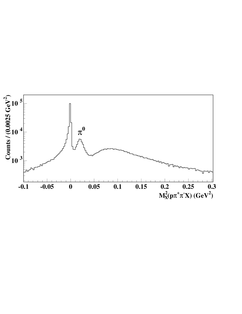
Some of the ”kaon” events are really misidentified $\pi^{+}$. This can be seen in Fig. 3 where all events are plotted assuming that all kaon candidates are really misidentified $\pi^{+}$ and compute the missing mass squared for the reaction $\gamma p\rightarrow p\pi^{+}\pi^{-}(X)$. The prominent spike at zero mass squared indicates $\gamma p\rightarrow p\pi^{+}\pi^{-}$ contamination and a $\pi^{0}$ peak is clearly evident but at a much reduced level. The expected distribution for good $K^{+}$ events goes to zero for zero $p\pi^{+}\pi^{-}$ missing mass squared. We require the missing mass squared from this calculation to be greater than 0.01 $GeV^{2}$ to eliminate for example $\rho\rightarrow\pi^{+}\pi^{-}$ contamination. We did not cut above the $\pi^{0}$ peak in Fig. 3 because that would have cut into the good $K^{+}$ events.

Figure 3: Pion contamination: Mass squared ($M_{X}^{2}$) for the $\gamma p\rightarrow p\pi^{+}\pi^{-}(X)$ reaction where the $\pi^{+}$ was a potentially mis-identified kaon.

The hadron mass spectrum after all of the above cuts have been applied are shown as the shadowed histogram in Fig. 2.

The kaon momentum is corrected for average dE/dx losses in the target material, target wall, carbon epoxy pipe and the start counter depending on the position of the primary vertex, which is approximated by the intersection of the proton and kaon tracks. The ground-state $\Lambda$ is sufficiently long-lived that it decays a measurable distance from the primary vertex. The secondary vertex is determined by the intersection of the proton and $\pi^{-}$ tracks. The proton and $\pi^{-}$ tracks are corrected for average dE/dx losses according to the position of the secondary vertex.

The four-momentum of the $\Lambda(1116)$ was reconstructed from the proton and $\pi^{-}$ four-momenta (Fig. 4). The Gaussian resolution of the $\Lambda$ peak is about $\sigma=1.3$ MeV, consistent with the instrumental resolution. The excited-state hyperon mass spectrum for the region between 1.25 GeV and 1.75 GeV requiring the $p\pi^{-}$ invariant mass to be in the range 1.112–1.119 GeV is shown in Fig. 5A. Fig. 5B shows the mass $M_{X}$ from the reaction $\gamma p\rightarrow\Lambda(X)$. A clear peak at the mass of the $K^{*}(892)$ is seen. The peak at the $K^{+}$ mass is due to accidentals under the TOF peak. This background is eliminated by requiring $M_{X}>0.55$ GeV. Fig. 6 shows the missing mass squared for the reaction $\gamma p\rightarrow K^{+}\Lambda(X)$ after the foregoing cuts have been applied. A prominent peak shows up at $M_{\pi^{0}}^{2}$ and a smaller peak at zero missing mass squared. The counts above the $\pi^{0}$ peak are typically due to $\gamma p\rightarrow K^{+}\Sigma^{0}(X)$.

Figure 4: $\Lambda$ identification: proton-$\pi^{-}$ invariant mass

Figure 5: (A) Missing mass for the reaction $\gamma p\rightarrow K^{+}(X)$. (B) Missing mass for the reaction $\gamma p\rightarrow\Lambda(X)$.

Figure 6: Missing mass squared for the reactions $\gamma p\rightarrow K^{+}\Lambda(X)$.

II.2 Kinematic fitting

A better approximation to the primary and secondary vertices can be found using kinematic fitting. We used the Lagrange multiplier method frodesen . The unknowns are divided into a set of measured variables ($\vec{\eta}$) and a set of unmeasured variables ($\vec{\xi}$) such as the missing momentum or the 4-vector for a decay particle. For each constraint equation a Lagrange multiplier $\lambda_{i}$ is introduced. We minimize

$$\chi^{2}(\vec{\eta},\vec{\xi},\vec{\lambda})=(\vec{\eta}_{0}-\vec{\eta})^{T}V^{-1}(\vec{\eta}_{0}-\vec{\eta})+2\vec{\lambda}^{T}\vec{f}$$ (4)

by differentiating $\chi^{2}$ with respect to all the variables, linearizing the constraint equations and iterating. Here $\vec{\eta}_{0}$ is a vector containing the initial guesses for the measured quantities and $V$ is the covariance matrix comprising the estimated errors on the measured quantities. We iterate until the difference in magnitude between the current $\chi^{2}$ and the previous value is $\leq$0.001. The covariance matrix $V$ for each track returned by the tracking code does not contain the effects of multiple scattering and energy loss in the target cell, the carbon epoxy pipe, or the start counter. To correct for this we apply multiple scattering and energy loss corrections to the diagonal matrix elements.

The first step in the fitting procedure is to fit the proton and $\pi^{-}$ tracks with the $\Lambda$ hypothesis. This is a 2C fit. There are six unknowns ($\vec{p}_{\Lambda}$, $\vec{r}_{V2}$) and eight constraint equations,

$$\vec{f}=\left[\begin{array}[]{c}E_{p}+E_{\pi}-E_{\Lambda}\\ \vec{p}_{p}+\vec{p}_{\pi}-\vec{p}_{\Lambda}\\ (y-y_{\pi})p^{z}_{\pi}-(z-z_{\pi})p^{y}_{\pi}\\ (x-x_{\pi})p^{z}_{\pi}-(z-z_{\pi})p^{x}_{\pi}\\ (y-y_{p})p^{z}_{p}-(z-z_{p})p^{y}_{p}\\ (x-x_{p})p^{z}_{p}-(z-z_{p})p^{x}_{p}\\ \end{array}\right]=\vec{0}.$$ (5)

The $\chi^{2}$ distribution for this fit is shown in Fig. 7A and the Confidence Level plot is shown in Fig. 7B. The curve is the result of a fit to the histogram using the function form of a $\chi^{2}$ distribution with two degrees of freedom plus a flat background term. Explicitly,

$$f(\chi^{2})=\frac{P_{1}}{2}e^{-P_{2}\chi^{2}/2}+P_{3}.$$ (6)

The fit result ($P_{2}=0.558$) suggests that we are underestimating the errors in the proton and $\pi^{-}$ tracks, but the shape is close to the expected shape. The Confidence Level is given by the equation

$$CL=\int_{\chi^{2}}^{\infty}f(z;n)dz$$ (7)

where f(z;n) is the $\chi^{2}$ probability density function with n degrees of freedom.

The second step is to use these Kaon and Lambda tracks to obtain a better primary vertex. This is a 1C fit. There are 3 unknowns ($\vec{r}_{V1}$) and four constraint equations. The $\chi^{2}$ distribution for this fit is shown in Fig. 7C and the Confidence Level plot is shown in Fig. 7D. The curve in Fig. 7C is the result of a fit to the histogram using the functional form of a $\chi^{2}$ distribution with one degree of freedom plus a flat background term. Explicitly,

$$f(\chi^{2})=\frac{P_{1}}{\sqrt{2}\ \Gamma(1/2)}\frac{e^{-P_{2}\chi^{2}/2}}{\sqrt{\chi^{2}}}+P_{3}.$$ (8)

with a fit result of $P_{2}=0.507$.

Figure 7: $\chi^{2}$ and Confidence Level distributions for the $\Lambda\rightarrow p\pi^{-}$ fit (A and B) and the $K^{+}\Lambda$ vertex fit (C and D).

We require the probability of the $\Lambda\rightarrow p\pi^{-}$ fit and the primary vertex fit be $\leq 0.5$% of exceeding $\chi^{2}$ for an ideal $\chi^{2}$ distribution. The improved kaon and lambda four vectors are used to compute the excited-state hyperon mass spectrum and the missing mass squared.

Fig. 8A compares the z-position of the primary vertex from the improved fitting procedure to the naive kaon-proton result.

Figure 8: A. Z-position of primary vertex. Solid histogram: K$\Lambda$ fit. Dashed histogram: Kp fit. B. Lambda decay proper time in units of $cm$. The excited-state hyperon mass was greater than 1.25 GeV for both plots.

We apply a target z-position cut for the primary vertex between -10.0 cm and +9.0 cm and a radial cut of 2 cm. These cuts were chosen to ensure that the primary event came from the target region. The proper time of the $\Lambda$ decay is plotted in Fig. 8B. An exponential fit to the data gives a decay constant of $7.62\pm 0.09$ cm which is comparable to the PDG value of 7.89$\pm$0.06 cm. To verify that the target walls do not make a significant contribution to our yields, we applied the analysis procedure described above to the empty-target data. For the empty target runs the beam current ranged between 10 and 24 nA and averaged about 15 nA. 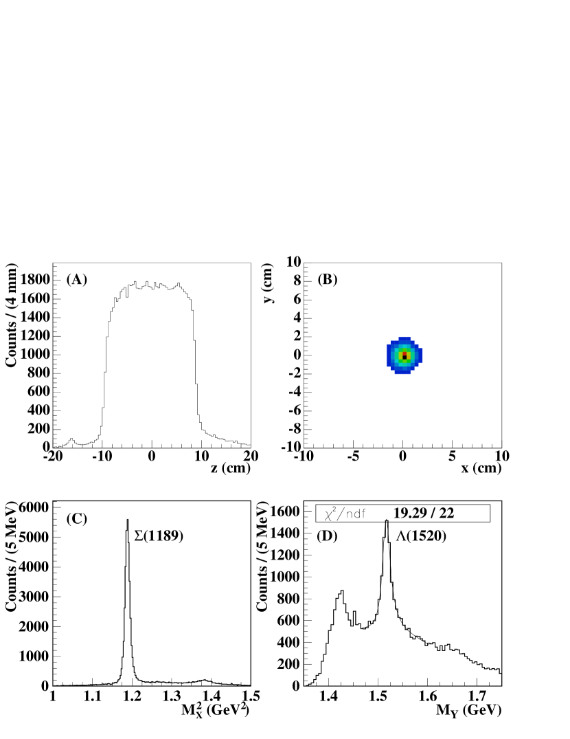The results from analyzing about 33 million empty-target events (corresponding to approximately $\frac{1}{3}$ of the target full integrated photon flux) are shown in Fig. 9. We obtained 25 $\Lambda(1116)$ candidates within the proton-$\pi^{-}$ invariant mass range of 1.112–1.119 GeV (Fig. 9A). The z distribution is shown in Fig. 9B. The hyperon mass distribution for those events satisfying the vertex cut is shown in Fig. 9C. Figure 9D shows the missing mass squared distribution for hyperon masses in the 1.34–1.43 GeV range. There are no counts near zero missing mass squared and only two near $m_{\pi^{0}}^{2}$. Both of these counts have z and r positions within the target volume. They correspond to interactions with the residual (cold) hydrogen gas in the target. From this we conclude that the background due to interactions with the walls of the target cell is negligible.

Figure 9: Empty target results. A. Proton piminus invariant mass. B. Vertex z-position. C. Hyperon mass. D. Missing mass squared for $M_{Y}$=1.34–1.43 GeV.

To achieve $\gamma/\pi^{0}$ separation, the events were sorted according to topology using kinematic fits with two hypotheses

R1:	$\gamma p\rightarrow K^{+}\Lambda\pi^{0}$	1C
R2:	$\gamma p\rightarrow K^{+}\Lambda\gamma$	1C

The corresponding constraint equations are

$$\vec{f}=\left[\begin{array}[]{c}E_{beam}+M_{p}-E_{K}-E_{\Lambda}-E_{X}\\ \vec{p}_{beam}-\vec{p}_{K}-\vec{p}_{\Lambda}-\vec{p}_{X}\end{array}\right]=\vec{0}.$$ (9)

Here X is a missing $\pi^{0}$ or a missing $\gamma$.

The $\chi^{2}$ distributions for reactions R1 and R2 are shown in Fig. 10A and 10C, respectively. The hyperon mass range was 1.25–1.75 GeV. The corresponding Confidence Levels plots are shown in Fig. 10B and 10D. For R1 we obtain the expected shape for a $\chi^{2}$ distribution with one degree of freedom. For R2 the $\chi^{2}$ values indicates that the radiative decay hypothesis is inconsistent with most of the events. The dashed curve in Figure 10D is the Confidence Level for hypothesis R2 for those events which do not satisfy hypothesis R1 at the 5% level. We now see a shape consistent with a $\chi^{2}$ distribution with one degree of freedom.

Figure 10: $\chi^{2}$ and Confidence Level distributions for the two reactions R1 (A and B) and R2 (C and D). The dashed curve in D is the R2 Confidence Level with the R1 reaction vetoed with $\chi^{2}$=3.841.

Fig. 11 shows the missing mass squared distributions for a representative set of $\chi^{2}$ cuts. For the purpose of the plot, we require $\chi^{2}_{R1}\geq 3.841$ and $\chi^{2}_{R2}<3.841$ to isolate the radiative channel (case B). To isolate the pion channel (case A), we require $\chi^{2}_{R1}<3.841$ and $\chi^{2}_{R2}\geq 3.841$. Case C is the “ambiguous” case where both $\chi^{2}_{R1}<3.841$ and $\chi^{2}_{R2}<3.841$. Case D consists of those events that do not agree with either the radiative channel or the pion channel, for which $\chi^{2}_{R1}\geq 3.841$ and $\chi^{2}_{R2}\geq 3.841$. For a 1C fit $\chi^{2}=3.841$ corresponds to a 5% probability of exceeding $\chi^{2}$ for an ideal $\chi^{2}$ distribution. The “ambiguous” events are most likely to be $\gamma p\rightarrow K^{+}\Lambda\pi^{0}$ events. Case D events are most likely be $\gamma p\rightarrow K^{+}\Sigma^{0}\pi^{0}$ events. Fig. 12 shows the corresponding hyperon mass spectra. Fig. 12A is dominated by the $\Sigma^{0}(1385)\rightarrow\Lambda\pi^{0}$ channel, for which the branching ratio is $\sim$88%pdg . We calculated the $\Sigma(1385)$ radiative transition relative to this channel. The $\Lambda(1520)$ peak shows up in Fig. 12D because of the decay channels $\Lambda(1520)\rightarrow\Sigma^{0}\pi^{0}$ (BR=14%) and $\Lambda(1520)\rightarrow\Lambda\pi\pi$ (BR=10%).

Figure 11: Missing mass squared distributions for $\chi^{2}_{HIGH}=\chi^{2}_{LOW}$ =3.841. Cases A–D are explained in the text.

Figure 12: Hyperon mass distributions for $\chi^{2}_{HIGH}=\chi^{2}_{LOW}$ = 3.841. Cases A-D are explained in the text.

II.3 Double Bremsstrahlung

The $\gamma$ channel does not show the structure expected from hyperon photon decays. The structure was found to be masked by a background resulting from double bremsstahlung in the radiator. The reaction $\gamma_{1}+\gamma_{2}p\rightarrow K^{+}\Lambda+\gamma_{1}$ can mimic the reaction $\gamma p\rightarrow K^{+}\Lambda\gamma$. But in this case the missing momentum from the reaction $\gamma p\rightarrow K^{+}\Lambda(X)$ points along the +z direction (along the beam). This can also happen if the event is an accidental or inefficiencies in the tagger plane allow the wrong electron to be selected. This problem is illustrated in Fig. 13. Fig. 13A shows the off-z-axis momentum $p_{\perp}^{2}=p_{x}^{2}+p_{y}^{2}$ for the candidate missing particle.

Figure 13: Effect of $p_{\perp}^{2}$ cut on $\gamma$ channel. A. The $p_{\perp}^{2}$ momentum spectrum for $K^{+}\Lambda(X)$ events. B. The $\gamma$ channel cut distibution for a 0.0004 GeV² cut. C. The $p_{\perp}^{2}$ momemtum spectrum for $K^{+}\Sigma^{0}(X)$ events. D. The $\gamma$ channel cut distibution for a 0.015 GeV² cut.

This misidentification should happen for ground-state $\Sigma^{0}(1193)$ production as well. A subset of the data filtered on the hyperon mass region between 1.0 and 1.25 GeV, was used to isolate $\Sigma^{0}(1193)$ events. The $\sigma$ from a Gaussian fit to the $\Sigma^{0}$ peak is about 6.6 MeV, corresponding to a full width at half maximum of $\Gamma=2.354\sigma=15.6$ MeV. This is a measure of the hyperon mass resolution. Apart from the hyperon mass range, the same set of cuts was used to analyze these data as for the excited-state sample. Fig. 13C shows the distribution in $p_{\perp}^{2}$ for this data set. Figures 13B and 13D compare the effect of two choices for the $p_{\perp}^{2}$ cut on the hyperon mass distribution for the case where the $\gamma$ channel is favored. The histograms show the distributions in hyperon mass for those events that were cut out. Histograms 13B and 13D both look like exponentially falling distributions. Fig. 14 shows the corresponding hyperon mass spectra after applying the $p_{\perp}^{2}=0.015\ GeV^{2}$ cut. The histogram now shows the expected structure for the $\Sigma(1385)\rightarrow\Lambda\gamma$ and $\Lambda(1520)\rightarrow\Lambda\gamma$ reactions. Comparison with 12A shows that this cut also reduces the number of $\Lambda\pi^{0}$ events seen. The Monte Carlo simulation III is used to correct for this reduction. The $p_{\perp}^{2}=0.015\ GeV^{2}$ cut will be used for the rest of the analysis.

Figure 14: Hyperon mass distributions for $\chi^{2}_{LOW}=\chi^{2}_{HIGH}=3.841$ with $p_{\perp}^{2}=0.015\ GeV^{2}$ cut. The labels are explained in the text. The yield of $\Lambda\pi^{0}$ and $\Lambda\gamma$ events in A and B were extracted by fitting the data with a relativistic Breit-Wigner (solid line) and a polynomial background (dashed line). In D the dashed histogram shows the contribution due to the $\Sigma(1385)$ alone. The dotted histogram is the $\Lambda(1405)$ contribution alone using the M-matrix parameterization for the shape.

III Acceptance

A detailed Monte Carlo simulation of the CLAS detector was performed using GEANT 3.21 for each of the three electron beam energies. Table 3 lists the set of reactions for which we generated events. The experimental photon energy distribution was used to determine the energies of the incident photons in the simulation. Relativistic Breit-Wigner shapes were used for the $\Sigma(1385)$, $\Lambda(1520)$ and $K^{*}$ mass distributions. For the $\Lambda(1520)$ the exponential slope for the t-dependence was 2.0 $GeV^{-2}$. The angular distribution for the radiative decay of the $\Lambda(1520)$ in its rest frame was taken to be proportional to $5-3\cos^{2}\theta$ according to the result obtained by Mast, et al.mast . The same distribution was used for the $\Sigma\pi$ channels and for the $\Sigma(1385)$ decays. The model of Nacher, et al. Oset with a flat angular distribution was used for the $\Lambda(1405)$ decay channels.

The incident photon energy dependence and t-dependence were adjusted to fit the data for the $\Sigma(1385)$ reactions independently for each of the electron beam energies. The data and MC were cut on the $Y^{*}$ mass range of 1.34–1.43 GeV and on the $\pi^{0}$ peak found in Fig. 14A to isolate the $\Sigma(1385)\rightarrow\Lambda\pi^{0}$ channel. We plotted the ratio of the data/MC versus photon energy $E_{beam}$. The resultant curve was fitted with a function of the form $A/E_{beam}+B/E_{beam}^{2}$. We used this to modify the photon energy dependence of the $\Sigma(1385)$ production cross section in the MC. The above procedure was then iterated. The exponential slope parameter was varied until the MC and data $t$ distributions matched reasonably well. The exponential slope for the modified t-dependence was 1.0 $GeV^{-2}$. To check the quality of the simulation, we compared the momentum distributions for the Monte Carlo and the data for the kaon, proton, and pion tracks. The simulated events were analyzed with the same cuts described above. The results for the second iteration for the MC simulation are shown in Fig. 15.

Figure 15: Momentum and angular distributions for MC (dashed histograms) and data (points with error bars) for the 1.34–1.43 GeV hyperon mass region.

The agreement between the MC and the data for the pion, proton, and kaon momenta and the kaon lab angle is good.

Fig. 16 compares the data for the 1.49–1.55 GeV mass range and the missing mass squared in the range 0.018–0.075 $GeV^{2}$ to the $\Lambda(1520)\rightarrow\Sigma^{0}\pi^{0}$ Monte Carlo results. The MC results have been scaled by 0.185. The agreement between the MC and the measured momenta distributions is very good and the kaon angular distributions agree reasonably well.

Figure 16: Momentum and angular distributions for MC (dashed histograms) and data (points with error bars) for the 1.49–1.55 GeV hyperon mass region.

In order to check that the $p_{\perp}^{2}$ cut did not introduce a bias of the Monte Carlo results with respect to the data, we studied the yield of $\Sigma(1385)\rightarrow\Lambda\pi^{0}$ events in the data and the corresponding Monte Carlo. For the data we used the standard $\chi^{2}$ cuts and performed the same kind of fit to the hyperon mass distributions as described earlier. The hyperon mass range was 1.34–1.43 GeV. The results are tabulated in table 2.

$p_{\perp}^{2}$ cut $(GeV^{2})$	N(data)	N(MC)	N(data)/N(MC)
0.005	4021	11037	0.364$\pm$0.007
0.010	3500	9860	0.355$\pm$0.007
0.015	2878	8148	0.353$\pm$0.008
0.020	2191	6191	0.354$\pm$0.009

Table 2: Comparison of yields between the $\Sigma(1385)\rightarrow\Lambda\pi^{0}$ simulation and the data as a function of the $p_{\perp}^{2}$ cut. The errors are statistical only.

The data and the MC yields agree as a function of the $p_{\perp}^{2}$ cut.

Table 3 lists the acceptances for the case where $\chi^{2}_{HIGH}=\chi^{2}_{LOW}=3.841$.

Reaction	$A_{\pi}$	$A_{\gamma}$	$A_{\gamma\pi}$
$\Lambda(1405)\rightarrow\Sigma^{0}\pi^{0}$	0.083$\pm$0.004	0.0007$\pm$0.0004	0.658$\pm$0.012
$\Lambda(1405)\rightarrow\Sigma^{+}\pi^{-}$	0.088$\pm$0.005	0.0038$\pm$0.0009	0.013$\pm$0.002
$\Lambda(1405)\rightarrow\Lambda\gamma$	0.008 $\pm$0.003	0.946$\pm$0.028	0.098$\pm$0.009
$\Lambda(1405)\rightarrow\Sigma^{0}\gamma$	0.585$\pm$0.019	0.380$\pm$0.015	0.837$\pm$0.023
$\Sigma(1385)\rightarrow\Lambda\pi$	0.905$\pm$0.010	0.011$\pm$0.001	0.086$\pm$0.003
$\Sigma(1385)\rightarrow\Sigma^{+}\pi^{-}$	0.050$\pm$0.002	0.0018$\pm$0.0005	0.00564$\pm$0.0008
$\Sigma(1385)\rightarrow\Lambda\gamma$	0.012$\pm$0.002	1.309$\pm$0.022	0.105$\pm$0.006
$\Sigma(1385)\rightarrow\Sigma^{0}\gamma$	0.548$\pm$0.016	0.24$\pm$0.01	0.99$\pm$0.02
$\Lambda(1520)\rightarrow\Lambda\gamma$		1.388$\pm$0.027	0.0010$\pm$0.0007
$\Lambda(1520)\rightarrow\Sigma^{0}\gamma$		0.087$\pm$0.006	0.586$\pm$0.016
$\Lambda(1520)\rightarrow\Lambda\pi^{0}\pi^{0}$		0	0.0099$\pm$0.0016
$\Lambda(1520)\rightarrow\Sigma^{0}\pi^{0}$		0.0006$\pm$0.0004	0.681$\pm$0.014

Table 3: Acceptances (in units of $10^{-3}$) for the channels used in the calculation of the branching ratios. Here $\chi^{2}_{HIGH}=\chi^{2}_{LOW}=3.841$. The uncertainties are statistical only.

In the table $A_{\pi}$ and $A_{\gamma}$ refer to the fraction of surviving events relative to the number of thrown events that satisfy the $\Lambda\pi^{0}$ and $\Lambda\gamma$ hypotheses, respectively, and $A_{\gamma\pi}$ refers to those events that do not satisfy either hypothesis.

IV $\Sigma^{0}(1385)$ Analysis

To obtain the yields we fitted the hyperon mass distributions between 1.25 GeV and 1.75 GeV. The yield of $\Lambda\pi^{0}$ events is extracted by fitting the data in Fig. 14A with a polynomial background and a relativistic Breit-Wigner of the form jackson

$$f(M)\propto\frac{2MM_{0}\Gamma(q)}{(M^{2}-M_{0}^{2})^{2}+M_{0}^{2}\Gamma^{2}(q)},$$ (10)

$$\Gamma(q)=\Gamma_{0}\left(\frac{q}{q_{0}}\right)^{2l+1}\frac{M_{0}}{M}\left(\frac{X_{0}^{2}+q_{0}^{2}}{X_{0}^{2}+q^{2}}\right)^{l},$$ (11)

$$q={\sqrt{(M^{2}-M_{\Lambda}^{2}-M_{\pi}^{2})^{2}-4M_{\Lambda}^{2}M_{\pi}^{2}}\over 2M},$$ (12)

$$q_{0}={\sqrt{(M_{0}^{2}-M_{\Lambda}^{2}-M_{\pi}^{2})^{2}-4M_{\Lambda}^{2}M_{\pi}^{2}}\over 2M_{0}},$$ (13)

where $M_{0}$ is the peak position of the resonance, $X_{0}$=0.35 GeV and $\Gamma_{0}$ is the width. For the $\Sigma^{*}\rightarrow\Lambda\pi^{0}$ transition, $l=1$. We tried both first order and second order polynomial background parameterizations. The systematic uncertainty in the yield extraction due to the choice of background function was about $\pm$1%. The mass and width of the $\Sigma(1385)$ were found to be 1.3860 GeV and 0.03988 GeV. For the $\Lambda\gamma$ channel (Fig. 14B), we used two relativistic Breit-Wigners (one for the $\Sigma(1385)$ and one for the $\Lambda(1520)$) plus a polynomial background. The masses and widths were fixed to be those found from the fits to Figures 14A and 14D.

From Fig.5A it is clear that we were not able to resolve the $\Lambda(1405)$ and the $\Sigma^{0}(1385)$, therefore in order to find the number of $\Lambda(1405)$’s ($n_{\Lambda}$) we look at the events for which neither the $\gamma$ nor the $\pi^{0}$ hypothesis is satisfied (Fig. 12D). This isolated predominantly $\Lambda(1405)\rightarrow\Sigma^{0}\pi^{0}$ events, since the $\Sigma(1385)\rightarrow\Sigma^{0}\pi^{0}$ decay is forbidden by isospin. We parameterized the $\Lambda(1405)$ line shape using the M-matrix formalism for S-wave $\Sigma^{0}\pi^{0}$ scattering below the $\overline{K}N$ threshold. The M-matrix is related to the S-wave transition matrix $T$ according to

$$T=Q^{\frac{1}{2}}(M-iQ)^{-1}Q^{\frac{1}{2}},$$ (14)

where $Q$ is a diagonal matrix containing the relative $\Sigma^{0}\pi^{0}$ momentum $q$ and $\overline{K}N$ momentum $k$ Thomas . Note that below the $\overline{K}N$ threshold, the latter is purely imaginary. The matrix $M$ is expanded relative to the $\overline{K}N$ threshold $E_{t}=M_{\overline{K}}+M_{N}$ according to

$$M(E)=M(E_{t})+\frac{1}{2}R(Q^{2}(E)-Q^{2}(E_{t}))$$

$$=\left[\begin{array}[]{cc}M_{11}&M_{12}\\ M_{12}&M_{22}\end{array}\right],$$ (17)

$$Q=\left[\begin{array}[]{cc}k&0\\ 0&q\end{array}\right],$$ (20)

$$R=\left[\begin{array}[]{cc}R_{\overline{K}N}&0\\ 0&R_{\Sigma\pi}\end{array}\right].$$ (23)

The amplitude for elastic scattering in the $\Sigma^{0}\pi^{0}$ channel is given by

$$T_{22}={q(M_{11}+|k|)\over(M_{11}+|k|)(M_{22}-iq)-M_{12}^{2}}.$$ (24)

Below $E_{t}$, the $\Sigma\pi$ mass spectrum is proportional to $|T_{22}|^{2}/q$. Fig. 14D shows the M-matrix parameterization fit to hyperon mass spectrum. A relativistic Breit-Wigner form is included to account for the leakage of the $\Sigma(1385)\rightarrow\Lambda\pi^{0}$ channel into the high missing mass squared region. A second relativistic Breit-Wigner is used for the $\Lambda(1520)$ contribution. The mass and width of the $\Lambda(1520)$ were found to be 1.520 GeV and 0.022 GeV. We used a second-order polynomial for the remaining background beneath the peaks. The matrix elements at threshold and the effective ranges were determined from the fit to be $M_{11}(E_{t})=1.314$, $M_{12}(E_{t})=-1.063$, $M_{22}(E_{t})=0.686$, $R_{\overline{K}N}=9.543$, and $R_{\Sigma\pi}=-28.89$. We find 328$\pm$36 $\Lambda(1405)$ counts and 245$\pm$37 $\Sigma(1385)$ counts in the hyperon mass region 1.34–1.43 GeV. The reduced $\chi^{2}$ for the fit was 0.866.

Reaction	Yield
Estimated $\Sigma^{0}\pi^{0}$ counts	373.8$\pm$34.0
Raw $\pi^{0}$ counts	2878.3$\pm$77.4
$\Lambda(1405)\rightarrow\Sigma^{0}\gamma$	0.45$\pm$0.17
$\Lambda(1405)\rightarrow\Sigma\pi$	95.7$\pm$9.5
$\Sigma(1385)\rightarrow\Sigma\pi$	10.4$\pm$1.0
$\Sigma(1385)\rightarrow\Lambda\gamma$	0.87$\pm$0.21
Corrected $\pi^{0}$ counts	2770.9$\pm$78.0
Raw $\gamma$ counts	100.2$\pm$15.4
$\Sigma(1385)\rightarrow\Lambda\pi^{0}$	35.0$\pm$1.0
$\Sigma(1385)\rightarrow\Sigma^{+}\pi^{-}$	0.38$\pm$0.3
$\Lambda(1405)\rightarrow\Lambda^{0}\gamma$	0.85$\pm$0.27
$\Lambda(1405)\rightarrow\Sigma^{0}\gamma$	0.29$\pm$0.11
$\Lambda(1405)\rightarrow\Sigma\pi$	2.47$\pm$0.25
Corrected $\gamma$ counts	61.2$\pm$15.4

Table 4: Breakdown of statistics for the $\Lambda\gamma$ and $\Lambda\pi^{0}$ channels. The errors are statistical only.

Although the $\pi^{0}$ leakage into the $\gamma$ channel is the dominant correction to the branching ratio, the final result still needs corrections for $\Sigma^{+}\pi^{-}$ contamination and the contribution to the numerator from the reaction $\Lambda(1405)\rightarrow\Lambda\gamma$. Based on the measured 27$\pm$8 keV radiative widthBurkhardt , we assume that the leakage of the $\Sigma\gamma$ channel into the $\gamma$ region is small relative to the $\Lambda\gamma$ signal and that the leakage into the $\pi^{0}$ region is small compared to the $\Lambda\pi^{0}$ signal. The formula for the acceptance corrected branching ratio is

$$R = \frac{1}{\Delta n_{\pi}A^{\Sigma}_{\gamma}(\Lambda\gamma)-\Delta n_{\gamma}A^{\Sigma}_{\pi}(\Lambda\gamma)}$$ (25)

$$\times\left[\Delta n_{\gamma}\left(A^{\Sigma}_{\pi}(\Lambda\pi)+\frac{R^{\Sigma\pi}_{\Lambda\pi}}{2}A^{\Sigma}_{\pi}(\Sigma\pi)\right)\right.$$

$$\left.-\Delta n_{\pi}\left(A^{\Sigma}_{\gamma}(\Lambda\pi)+\frac{R^{\Sigma\pi}_{\Lambda\pi}}{2}A^{\Sigma}_{\gamma}(\Sigma\pi)\right)\right],$$

$$\Delta n_{\pi} = n_{\pi}-N_{\pi}(\Lambda^{*}\rightarrow\Sigma^{+}\pi^{-})-N_{\pi}(\Lambda^{*}\rightarrow\Sigma^{0}\pi^{0})$$ (26)

$$-N_{\pi}(\Lambda^{*}\rightarrow\Sigma^{0}\gamma)-N_{\pi}(\Lambda^{*}\rightarrow\Lambda\gamma),$$

$$\Delta n_{\gamma} = n_{\gamma}-N_{\gamma}(\Lambda^{*}\rightarrow\Sigma^{+}\pi^{-})-N_{\gamma}(\Lambda^{*}\rightarrow\Sigma^{0}\pi^{0})$$ (27)

$$-N_{\gamma}(\Lambda^{*}\rightarrow\Sigma^{0}\gamma)-N_{\gamma}(\Lambda^{*}\rightarrow\Lambda\gamma),$$

where $n_{\gamma}$ ($n_{\pi}$) is the measured number of photon (pion) candidates and the remaining $N_{\gamma,\pi}$ terms are corrections due to leakage from the $\Lambda(1405)$. The acceptance for the individual pion (photon) channels are denoted as $A^{\Sigma}_{\pi}(\Sigma^{+}\pi^{-})$, ($A^{\Sigma}_{\gamma}(\Sigma^{+}\pi^{-})$) and so on. For example, $A^{\Sigma}_{\gamma}(\Lambda\pi)$ denotes the relative leakage of the $\Lambda\pi$ channel into the $\Lambda\gamma$ channel. Table 3 lists the values of these “acceptances”.

The corrections depend on an estimate of the number $n_{\Lambda}$ of $\Lambda(1405)$’s in the data set. They are

$$N_{\gamma}(\Lambda^{*}\rightarrow\Lambda\gamma) = \frac{A^{\Lambda}_{\gamma}(\Lambda\gamma)R(\Lambda^{*}\rightarrow\Lambda\gamma)n_{\Lambda}}{A^{\Lambda}_{\gamma\pi}(\Sigma^{0}\pi^{0})+A^{\Lambda}_{\gamma\pi}(\Sigma^{+}\pi^{-})},$$ (28)

$$N_{\gamma}(\Lambda^{*}\rightarrow\Sigma^{0}\gamma) = \frac{A^{\Lambda}_{\gamma}(\Sigma^{0}\gamma)R(\Lambda^{*}\rightarrow\Sigma^{0}\gamma)n_{\Lambda}}{A^{\Lambda}_{\gamma\pi}(\Sigma^{0}\pi^{0})+A^{\Lambda}_{\gamma\pi}(\Sigma^{+}\pi^{-})},$$ (29)

$$N_{\gamma}(\Lambda^{*}\rightarrow\Sigma^{0}\pi^{0}) = \frac{A^{\Lambda}_{\gamma}(\Sigma^{0}\pi^{0})n_{\Lambda}}{A^{\Lambda}_{\gamma\pi}(\Sigma^{0}\pi^{0})+A^{\Lambda}_{\gamma\pi}(\Sigma^{+}\pi^{-})},$$ (30)

$$N_{\gamma}(\Lambda^{*}\rightarrow\Sigma^{+}\pi^{-}) = \frac{A^{\Lambda}_{\gamma}(\Sigma^{+}\pi^{-})n_{\Lambda}}{A^{\Lambda}_{\gamma\pi}(\Sigma^{0}\pi^{0})+A^{\Lambda}_{\gamma\pi}(\Sigma^{+}\pi^{-})},$$ (31)

and similarly for the pion channel. Here isospin symmetry is assumed such that $R(\Sigma^{0}\pi^{0})=R(\Sigma^{+}\pi^{-})=R(\Sigma^{-}\pi^{+})\approx 1/3$ for the $\Lambda(1405)$ decay channels. The subscript “$\gamma\pi$” refers to those events for which both a pion and a photon are missing or those events leaking into the “$\gamma\pi$” region due to the tail of the $\pi^{0}$ peak (this is why the $\Sigma^{+}\pi^{-}$ contamination must be included in the denominator, although the leakage for this channel is small). Table 4 lists the yields for the various channels of the $\Sigma(1385)$ decays. The hyperon mass range was 1.34–1.43 GeV. The reaction $\gamma p\rightarrow\Lambda K^{*+}$ causes a smooth background underneath the $\Sigma(1385)$ peak in Figures 14A and 14B that is well parameterized by the second order polynomial fit. Hence it has not been explicitly included Table 4. The largest background in the $\gamma$ channel is due to leakage of the $\pi^{0}$ tail into the $\gamma$ missing mass squared region.

After subtracting the background contributions enumerated in table 4 there were $61.2\pm 15.4$ counts consistent with $\Sigma^{0}(1385)\rightarrow\Lambda\gamma$ and $2770.9\pm 78.0$ counts consistent with $\Sigma^{0}(1385)\rightarrow\Lambda\pi^{0}$. After correcting for the relative acceptance of the two channels, we obtained a branching ratio, $R^{\Lambda\gamma}_{\Lambda\pi}$, of

$$\frac{\Gamma(\Sigma^{0}(1385)\rightarrow\Lambda\gamma)}{\Gamma(\Sigma^{0}(1385)\rightarrow\Lambda\pi^{0})}=1.53\pm 0.39(\mathrm{stat})\%.$$ (32)

The branching ratio result for the $\Sigma(1385)$ depends on how well we understand the tail of the $\pi^{0}$ peak near the $\gamma$ peak. Fig. 17C and 17D shows the comparison between the data and the Monte Carlo for the reaction $Y^{*}\rightarrow\Lambda X$ for the 1.34–1.43 GeV hyperon mass region. The excess of counts above the $\pi^{0}$ peak correspond to $Y\to\Sigma^{0}\pi^{0}$, where $\Sigma^{0}\to\Lambda\gamma$. Although the $Y\to\Lambda\gamma$ decay is not completely separated, a clear enhancement near zero missing mass squared can be seen above the $\pi^{0}$ tail clearly indicating the presence of radiative events. The Monte Carlo predicts that the leakage accounts for about 30% of the raw photon yield in the $|M_{X}^{2}|<0.01$ GeV² region. In order to assess the quality of the Monte Carlo in the tail, we looked at $\Lambda(1405)\rightarrow\Sigma^{+}\pi^{-}$ events for which the $\Sigma^{+}$ subsequently decayed to $p\pi^{0}$. We chose this channel because there are no channels that can distort the spectrum above the $\pi^{0}$ peak, the $\Sigma^{+}$ radiative channel is rare ($BR=1.25\times 10^{-3}$), and has similar kinematics to the $\Lambda\pi^{0}$ decay. We required the $p\pi^{-}$ invariant mass to be greater than 1.13 GeV (to eliminate the $\Lambda(1116)$ from the sample). To identify the $\Sigma^{+}(1189)$ we require the $pX$ invariant mass (or, equivalently, the missing mass recoiling off the $K^{+}\pi^{-}$ system) to be in the range 1.17-1.206 GeV. We performed kinematic fits on these events with vertex and four-momentum conservation constraints. Explicitly, the constraint equations are

$$\vec{f}=\left[\begin{array}[]{c}E_{beam}+m_{p}-E_{K}-E_{\pi}-E_{\Sigma^{+}}\\ \vec{p}_{beam}-\vec{p}_{\pi}-\vec{p}_{p}-\vec{p}_{\Sigma^{+}}\\ (y-y_{\pi})p^{z}_{\pi}-(z-z_{\pi})p^{y}_{\pi}\\ (x-x_{\pi})p^{z}_{\pi}-(z-z_{\pi})p^{x}_{\pi}\\ (y-y_{p})p^{z}_{K}-(z-z_{p})p^{y}_{K}\\ (x-x_{p})p^{z}_{K}-(z-z_{p})p^{x}_{K}\\ \end{array}\right]=\vec{0}.$$ (33)

The missing mass squared distribution for the reaction chain $Y^{*}\rightarrow\Sigma^{+}\pi^{-}$, $\Sigma^{+}\rightarrow p(X)$ is shown in Fig. 17C and 17D for hyperon masses in the 1.38–1.45 GeV mass region. We used the four-vector for the $\Sigma^{+}$ obtained from the fit, with less than 0.5% probability of exceeding $\chi^{2}$. The Monte Carlo result (dashed histograms) for the $\Lambda(1405)\rightarrow\Sigma^{+}\pi^{-}$ reaction agrees very well with the data down to about zero missing mass squared. The discrepancy between the MC and the data in the $-$0.01 – +0.01 $GeV^{2}$ region is about $\sim 19\%$. Scaling the leakage of the $\Lambda\pi^{0}$ channel into the $\gamma$ region by a factor of 1.19 reduces the branching ratio from 1.53% to 1.36% for a relative change of about $-$11%. More importantly, comparing 17B with 17D shows a clear enhancement at zero missing mass present for the latter case not in evidence for the former case. The negative systematic error will be increased by 11% in quadrature.

Figure 17: Comparison between data and Monte Carlo results for the reactions and $Y^{*}\rightarrow\Lambda X$ (top histograms) $Y^{*}\rightarrow\Sigma^{+}\pi^{-}$ (bottom histograms) after kinematic fitting has been performed. The points with error bars are the data and the curves are the MC results. Histrograms B and D have the vertical scales expanded by a factor of ten. In B the solid curve on the left is the $\Sigma^{*}\rightarrow\Lambda\gamma$ simulation, the central dashed curve is the $\Sigma^{*}\rightarrow\Lambda\pi^{0}$ simulation, the isolid curve on the right is the $\Lambda(1405)\rightarrow\Sigma^{0}\pi^{0}$ simulation. In A the curve is the sum of the three. In C and D the $\Sigma^{+}\pi^{-}$ data and the $\Sigma(1385)\rightarrow\Lambda\pi^{0}$ Monte Carlo distribution have been scaled to agree with the peak height of the $\pi^{0}$ in the $Y^{*}\rightarrow\Lambda X$ distribution from the data set.

V $\Lambda(1520)$ analysis

For the $\Lambda(1520)$ analysis we calculated the radiative branching ratio relative to the $\Sigma^{0}\pi^{0}$ and the $\Sigma^{+}\pi^{-}$ channels. The hyperon mass cut used to identify the $\Lambda(1520)$ was 1.49-1.55 GeV. From the fit to the histogram shown in Fig. 14, we obtained $n_{\gamma}=32.5\pm 8.2$. To identify the $\Sigma^{0}\pi^{0}$ channel we used events for which neither the $\gamma$ nor the $\pi^{0}$ hypothesis is satisfied. The ground-state $\Lambda$ is a decay product in the $\Sigma^{0}\pi^{0}$ (14%) and $\Lambda\pi\pi$ (10%) channels. In order to simplify the calculation for the branching ratio we require the missing mass squared to be in the range between $m_{\pi^{0}}^{2}$ and 0.075 $GeV^{2}$ ($\approx 4m_{\pi^{0}}^{2}$, the two-pion threshold). This isolates the $\Sigma^{0}\pi^{0}$ channel. The hyperon mass distribution in the $\Lambda(1520)$ region with this additional cut applied is shown in Fig. 18.

Figure 18: Sample fit of the $\Lambda X$ mass distribution for missing mass squared in the 0.018-0.075 $GeV^{2}$ range.

The fit is a D-wave ($l=2$) relativistic Breit-Wigner plus a polynomial background. We tried both first-order and second-order polynomials; the results for the yield differed by $\pm 1.6\%$.

Reaction	Yield
$\Lambda(1520)\rightarrow\Sigma^{+}\pi^{-}$	5290$\pm$124
$\Lambda(1520)\rightarrow\Sigma^{0}\pi^{0}$	202.8$\pm$16.7
$\Lambda(1520)\rightarrow\Lambda\gamma$	0.05$\pm$0.01
Corrected $\pi^{0}$ counts	202.8$\pm$16.7
Raw $\gamma$ counts	32.5$\pm$8.2
$\Lambda(1520)\rightarrow\Sigma^{0}\pi^{0}$	0.09$\pm$0.01
Corrected $\gamma$ counts	32.4$\pm$8.2

Table 5: Breakdown of statistics for the $\Lambda(1520)$ analysis. The errors are statistical only.

The leakage of one channel into the other is neglible and applying the correction does not change the result. Due to the low acceptance for events containing $\Lambda$’s, the raw number of $\Sigma^{0}\pi^{0}$ counts is only a factor of 6 larger than the radiative signal and the technique relies on isolating a channel for which two particles ($\gamma$ and $\pi^{0}$) are not detected. We also looked at $\Lambda(1520)\rightarrow\Sigma^{+}\pi^{-}$ events for which the acceptance is higher. The same particle identification and vertex cuts used for the previous analysis were applied with some modifications. We required that the $p\pi^{-}$ invariant mass be greater than 1.13 GeV to cut $\Lambda(1116)$ contamination. The primary vertex was determined using the $K^{+}$ and $\pi^{-}$ tracks. The z-position and x- and y-positions for these vertexes are shown in Fig. 19A and 19B, respectively.

Figure 19: Isolation of $Y^{*}\rightarrow\Sigma^{+}\pi^{-}$ events. A) and B) show the $K^{+}\pi^{-}$ vertex distributions. C) is the missing mass for the reaction $\gamma p\rightarrow K^{+}\pi^{-}X$. D) is the hyperon mass distribution for events satisfying the $\Sigma^{+}$ identification cut (see text).

A prominent $\Sigma^{+}(1189)$ peak shows up in the missing mass recoiling against the $K^{+}$ and the $\pi^{-}$ (Fig. 19C). The hyperon mass spectrum for those events in the range 1.165–1.215 GeV about the $\Sigma^{+}$ peak are shown in Fig. 19D. The curve is a fit to the $\Lambda(1520)$ region using a D-wave relativistic Breit-Wigner with a second-order polynomial background. In the region between 1.49 GeV and 1.55 GeV we obtain $n_{\Lambda^{*}}=5290\pm 124$ (the acceptance of CLAS is much larger for this channel than the others due to the larger $\pi^{-}$ momentum). The yields for these two reactions are listed in table 5. As can be seen from the numbers in the table the leakage of each channel into the other is negligible. None of the generated $\Lambda(1520)\rightarrow\Sigma^{+}\pi^{-}$ events satisfied the selection criteria. There is no $\Lambda\pi^{0}$ leakage since this channel is forbidden by isospin.

We obtained a raw branching ratio of $n_{\gamma}/n_{\gamma\pi}=16.0\pm 4.3\%$. Correcting for acceptance, the branching ratio is

$${\Gamma(\Lambda\gamma)\over\Gamma(\Sigma^{0}\pi^{0})}=\frac{A_{\gamma\pi}(\Sigma^{0}\pi^{0})}{A_{\gamma}(\Lambda\gamma)}\frac{n_{\gamma}}{n_{\gamma\pi}}=7.9\pm 2.1\%.$$ (34)

The acceptances used in this calculation are listed in table 3. To obtain the branching ratio $\Gamma(\Lambda\gamma)/\Gamma_{TOT}$ we scale this result by the branching fraction of 14% for the $\Sigma^{0}\pi^{0}$ channel (assuming isospin symmetry) to obtain 1.10$\pm$0.29%. The acceptance for the $\Lambda(1520)\rightarrow\Sigma^{+}\pi^{-}$ channel was $1.66\pm 0.06$%. We obtain $1.01\pm 0.26$% for the radiative branching ratio. The results for the two channels agree after acceptance corrections.

If contamination due to the $\Lambda(1520)\rightarrow\Sigma^{0}\gamma$ channel is present the branching ratio for the $\Lambda\gamma$ channel acquires a small correction term:

$$R(\Lambda\gamma) = \frac{A_{\gamma\pi}(\Sigma^{0}\pi^{0})}{A_{\gamma}(\Lambda\gamma)}\frac{n_{\gamma}}{n_{\gamma\pi}}R(\Sigma^{0}\pi^{0})$$ (35)

$$+R(\Sigma^{0}\gamma)\left({A_{\gamma\pi}(\Sigma^{0}\gamma)n_{\gamma}-A_{\gamma}(\Sigma^{0}\gamma)n_{\gamma\pi}\over A_{\gamma}(\Lambda\gamma)n_{\gamma\pi}}\right),$$

where $R(\Sigma^{0}\gamma)$ is the branching ratio to the $\Sigma^{0}\gamma$ channel and $R(\Sigma^{0}\pi^{0})$ is the branching ratio to the $\Sigma^{0}\pi^{0}$ channel. Using the largest theoretical estimate for the $\Sigma^{0}\gamma$ radiative width of 293 keV from Warns, et al.warns , we obtain a correction of +0.01%. Therefore this contamination can be neglected.

VI Results

To check the sensitivity to the confidence limits used, $R^{\Lambda\gamma}_{\Lambda\pi^{0}}$ was calculated with 1%, 5% and 10% probability for accepting a channel and 99%, 95% and 90% probability for rejecting a channel. Table 6 lists the corrected branching ratios as a function of the $\chi^{2}_{HIGH,LOW}$ cuts. The third column in Table 6 gives the $\Sigma(1385)$ results. The results were very stable, varing from +0.15 (10%, 90%) to $-$0.17 (5%, 99%). These values were used as estimates of the systematic errors. The value for the branching ratio is $1.53\pm 0.39(\mathrm{stat})^{+0.15}_{-0.17}(\mathrm{sys})$%, where the second uncertainty reflects the variation in the branching ratio as a function of the choice of $\chi^{2}$ cuts.

$\chi^{2}_{LOW}$	$\chi^{2}_{HIGH}$	R(%) $\Sigma(1385)$	R(%) $\Lambda(1520)$
2.706	2.706	1.68$\pm$0.41	1.20$\pm$0.29
3.841	3.841	1.53$\pm$0.39	1.10$\pm$0.29
6.635	6.635	1.58$\pm$0.40	1.13$\pm$0.33
2.706	6.635	1.38$\pm$0.38	1.25$\pm$0.33
3.841	6.635	1.36$\pm$0.30	1.06$\pm$0.34

Table 6: Dependence of the $\Sigma(1385)\rightarrow\Lambda\gamma$ and $\Lambda(1520)\rightarrow\Lambda\gamma$ branching ratio on the choice of $\chi^{2}_{HIGH,LOW}$ cuts.

We add the 11% relative error (i.e. $-$0.17% absolute) that could result from underestimating the tail of the $\pi^{0}$ response to the negative systematic error and quote a branching ratio of $1.53\pm 0.39(\mathrm{stat})^{+0.15}_{-0.24}(\mathrm{sys})$%. The positive systematic error reflects the range of values we obtained for the various estimates for the branching ratio. If we neglect the small (unmeasured) contribution due to the $\Sigma^{0}\gamma$ channel, the $\Sigma^{0}(1385)\rightarrow\Lambda\gamma$ partial width is given by

$$\Gamma(\Lambda\gamma)={R^{\Lambda\gamma}_{\Lambda\pi}\Gamma_{TOT}\over 1+R^{\Lambda\gamma}_{\Lambda\pi}+R^{\Sigma\pi}_{\Lambda\pi}}=479\pm 120(\mathrm{stat})^{+81}_{-100}(\mathrm{sys})\mbox{ keV},$$ (36)

using $\Gamma_{TOT}=36\pm 5$ MeV and $R^{\Sigma\pi}_{\Lambda\pi}=0.135\pm 0.011$, the branching ratio of the $\Sigma\pi$ channels relative to the $\Lambda\pi^{0}$ channelpdg . The errors on $\Gamma_{TOT}$ and $R^{\Sigma\pi}_{\Lambda\pi}$ are included in the systematic error for $\Gamma(\Lambda\gamma)$. If we use the largest theoretical estimate for the $\Sigma^{0}\gamma$ channel relative to the $\Lambda\gamma$ channel of 0.153 from R. Bijker, F. Iachello, and A. LeviatanBijker:2000gq , the partial width is reduced to 478 keV, which is an insignificant change.

For the $\Lambda(1520)$ decay, we obtained a branching ratio of $1.10\pm 0.29(\mathrm{stat})^{+0.15}_{-0.04}(\mathrm{sys})$% using the $\Sigma^{0}\pi^{0}$ channel and $1.01\pm 0.27$% using the $\Sigma^{+}\pi^{-}$ channel. The weighted average gives a branching ratio of

$$\frac{\Gamma(\Lambda(1520)\rightarrow\Lambda\gamma)}{\Gamma_{TOT}}=1.07\pm 0.29(\mathrm{stat})^{+0.15}_{-0.04}(\mathrm{sys})\%.$$ (37)

Table 6 lists the branching ratios for various combinations of kinematic fitting $\chi^{2}$ cuts. There is no obvious dependence on the choice of cuts. To determine the systematic error in the measurement using the $\Sigma^{0}\pi^{0}$ channel to normalize, we used the range of branching ratio values obtained for different choices of $\chi^{2}$ cuts. Using a full width of 15.6$\pm$1 MeVpdg , we obtain a partial width of $167\pm 43(\mathrm{stat})^{+26}_{-12}(\mathrm{sys})$ keV. The error on the full width is included in the systematic error for $\Gamma(\Lambda\gamma)$. The $\Lambda(1520)$ result is compatible with the Mast et al. resultmast and the Antipov et al. resultAntipov:2004qp but disagrees with the Bertini et al. resultbertini . Together, our result and those of Mast et al. and Antipov et al. exclude the bag models listed in Table 1.

The $\Sigma^{0}(1385)\rightarrow\Lambda\gamma$ channel has never been measured before. The result is roughly 2–3 times larger than all of the existing model predictions except for HB$\chi$PTbutler . Table 1 reveals that the model predictions for the $\Delta\rightarrow p\gamma$ transition are also about 50% low. Sato and Leesato showed that much of that discrepancy could be accounted for by the inclusion of non-resonant meson-exchange effects. They find a width of 530$\pm$45 keV, about 80% of the experimental value. Lu et al.lu reproduced the $\Delta\rightarrow p\gamma$ data using a chiral bag model calculation with a relatively small bag radius of 0.7 fm. About 40% of the transition was due to the pion cloud. These calculations suggest that mesonic effects could account for the discrepancy between the model predictions and our result for the $\Sigma^{0}(1385)$ radiative transition.

We would like to acknowledge the outstanding efforts of the staff of the Accelerator and the Physics Divisions at TJNAF that made this experiment possible. This work was supported in part by the Istituto Nazionale di Fisica Nucleare, the French Centre National de la Recherche Scientifique, the French Commissariat à l’Energie Atomique, the U.S. Department of Energy, the National Science Foundation, Emmy Noether grant from the Deutsche Forschungs Gemeinschaft and the Korean Science and Engineering Foundation. The Southeastern Universities Research Association (SURA) operates the Thomas Jefferson National Accelerator Facility for the United States Department of Energy under contract DE-AC05-84ER40150.