Abstract

We discuss the current status and the physics prospects at the LHCb detector, the dedicated B physics detector at the LHC, due to start data taking in 2007.

1 Introduction

LHCb is a dedicated B–physics experiment at the future LHC collider, making use of the large number of B–hadrons expected at the LHC. The experiment is scheduled to start data taking in 2007. Here we will introduce the LHCb detector, and its physics potential, focusing on one of its most exciting features, LHCb’s ability to perform precision measurements on the CKM angle $\gamma$ in many different decay channels, in both the ${\rm B_{s}^{0}}$ and the ${\rm B_{d}^{0}}$ system. This will thoroughly over constrain the Standard Model description of CP violation and provide a sensitive probe for New Physics.

A more detailed description of the LHCb detector and its projected physics performance can be found in the LHCb technical design reports [1].

2 CP Violation

2.1 CP Violation in the Standard Model

In the Standard Model, $\mathcal{CP}$ violation can be accommodated by a single complex phase $\delta_{13}$ in the CKM matrix, which is the matrix that relates the mass–eigenstates of the down–type quarks to the weak isospin partners of the up–type quarks:

$$V_{\mathrm{CKM}}=\left(\begin{array}[]{ccc}V_{ud}&V_{us}&V_{ub}\\ V_{cd}&V_{cs}&V_{cb}\\ V_{td}&V_{ts}&V_{tb}\end{array}\right).$$ (1)

The transition amplitudes between quarks are proportional to the corresponding elements in the CKM matrix, for example the amplitude for $d_{L}\to u_{L}$ is proportional to $V_{ud}$, while the CP-conjugate process, $\bar{d}_{R}\to\bar{u}_{R}$ is proportional to the complex conjugate, $V_{ud}^{\ast}$. Experimentally, it is found that the magnitudes of the CKM matrix elements follow a clear structure. In terms of the sine of the Cabibbo angle, $\lambda\equiv\sin\theta_{C}=0.22$, the order of magnitude of the CKM matrix elements is:

$$\left(\begin{array}[]{ccc}1&\lambda&\lambda^{3}\\ \lambda&1&\lambda^{2}\\ \lambda^{3}&\lambda^{2}&1\end{array}\right).$$ (2)

Up to $\mathcal{O}\!\left(\lambda^{3}\right)$ in the Wolfenstein parametrisation of the CKM matrix [16], only the two smallest elements have complex phases (these phases are not independent and would vanish if $\delta_{13}$ were 0):

$$V_{td}=\left|V_{td}\right|e^{-i\beta}\mbox{\hskip 30.00005pt and \hskip 30.00005pt}V_{ub}=\left|V_{ub}\right|e^{-i\gamma}.$$ (3)

At $\mathcal{O}\!\left(\lambda^{4}\right)$, another, phase appears, $\delta\gamma$:

$$V_{ts}=\left|V_{ts}\right|e^{-i\delta\gamma}.$$ (4)

All three phases up to $\mathcal{O}\!\left(\lambda^{4}\right)$, $\beta$, $\gamma$ and $\delta\gamma$, are accessible in B-systems. The phase $\gamma$ appears in all decays involving $b\to u$ transitions, for example ${\rm B_{d}\to\pi^{+}\pi^{-}}$ and ${\rm B_{s}\to K^{+}K^{-}}$. The phase $\beta$ appears in ${\rm B_{d}}$ mixing, where a ${\rm B_{d}}$ meson transforms into a ${\rm\bar{B}_{d}}$ meson: ${\rm B_{d}}\stackrel{{\scriptstyle-2\beta}}{{\longrightarrow}}{\rm\bar{B}_{d}}$. Analogously, the phase $\delta\gamma$ is the mixing angle of the ${\rm B_{s}}$ system, ${\rm B_{s}}\stackrel{{\scriptstyle-2\delta\gamma}}{{\longrightarrow}}{\rm\bar{B}_{s}}$. While $\beta$ and $\gamma$ are $\mathcal{O}\!\left(1\right)$, $\delta\gamma$ is expected to be $\mathcal{O}\!\left(10^{-2}\right)$ in the Standard Model.

The complex CKM elements result in phase differences between interfering decay paths to the same final state, one with and one without mixing, as illustrated in figure 1.

(a) ${\rm{\rm B_{d}^{0}}\to{\rm J\!/\!\psi}{\rm K_{S}}}$	(b) ${\rm{\rm B_{d}^{0}}\to{\rm\pi^{+}}{\rm\pi^{-}}}$
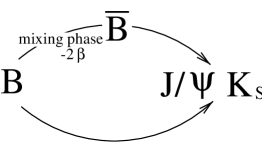
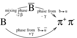
$\delta_{\mathrm{CP}}=-2\beta$	$\delta_{\mathrm{CP}}=-2\left(\beta+\gamma\right)$

Figure 1: The CKM phases are observable as phase differences between interfering decay paths to the same final state. Here illustrated for the examples ${\rm{\rm B_{d}^{0}}\to{\rm J\!/\!\psi}{\rm K_{S}}}$ (sensitive to $\sin 2\beta$) and ${\rm{\rm B_{d}^{0}}\to{\rm\pi^{+}}{\rm\pi^{-}}}$ (sensitive to $\sin(2\beta+2\gamma)$). This illustration ignores the penguin contributions to ${\rm{\rm B_{d}^{0}}\to{\rm\pi^{+}}{\rm\pi^{-}}}$, which are discussed later in the text.

These phase differences can be observed as the amplitudes of time dependent decay rate asymmetries, for example for ${\rm B\to J\!/\!\psi K_{s}}$:

$$A\!\left(\tau\right)=\frac{\Gamma\left({\rm{\rm B_{d}^{0}}\to{\rm J\!/\!\psi}K_{S}}\right)-\Gamma\left({\rm{\rm\overline{B_{d}^{0}}}\to{\rm J\!/\!\psi}K_{S}}\right)}{\Gamma\left({\rm{\rm B_{d}^{0}}\to{\rm J\!/\!\psi}K_{S}}\right)+\Gamma\left({\rm{\rm\overline{B_{d}^{0}}}\to{\rm J\!/\!\psi}K_{S}}\right)}=\sin\!\left(2\beta\right)\sin\!\left(\Delta\!m\tau\,\right),$$ (5)

where $\Delta\!m$ is the mass difference between the two ${\rm B_{d}^{0}}$ mass eigenstates, $\tau$ is the decay eigentime and the flavours ${\rm B_{d}^{0}}$ and ${\rm\overline{B_{d}^{0}}}$ refer to the flavour at the time of creation ($\tau=0$). An experiment measuring CP violation in the B systems would therefore require a good time (decay length) resolution, especially to resolve the rapid ${\rm B_{s}}$ oscillations. Also, because the branching fractions to CP sensitive decays are typically $\mathcal{O}\!\left(10^{-5}\right)$, large, clean data samples are required, and efficient B flavour tagging (the ability to identify the flavour of the B at the time of creation). LHCb is specifically designed to meet these requirements.

2.2 Unitarity Triangle

The only Standard Model prediction with respect to the CKM matrix is that it is unitary:

$$V_{\mathrm{CKM}}V_{\mathrm{CKM}}^{\dagger}=1\!\!1$$ (6)

This results in 9 equations. The most relevant one for CP violation in the B systems is

$$V_{ub}^{\ast}V_{ud}+V_{cb}^{\ast}V_{cd}+V_{tb}^{\ast}V_{td}=0.$$ (7)

which can also be written as:

$$\frac{V_{ub}^{\ast}V_{ud}}{V_{cb}^{\ast}V_{cd}}+1+\frac{V_{tb}^{\ast}V_{td}}{V_{cb}^{\ast}V_{cd}}=0.$$ (8)

Drawing these three numbers adding up to zero as points in the complex plane, results in the Unitarity Triangle.

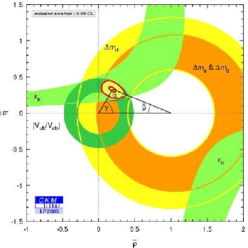
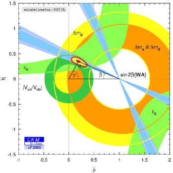
Without direct measurement	Including $\sin 2\beta$ measurement
of $\sin 2\beta$	from charmonium decays [14].

Figure 2: Current status of the Unitarity Triangle [13]. The $\bar{\rho}-\bar{\eta}$ plane is effectively the complex plane, using parameters of the improved [15] Wolfenstein [16] parametrisation. The angles $\beta$ and $\gamma$ correspond to the CP-violating phases introduced in Eq 3. The third angle $\alpha$ does not correspond to another complex entry in the CKM matrix, and is defined as $\alpha=\pi-\beta-\gamma$.

The normalised Unitarity Triangle (Eq 8) is fully described by the position of its apex in the complex plane. The angles correspond to the CKM-phases $\beta,\gamma$, introduced above. The third angle $\alpha$, often found in the literature, is given by $\alpha=\pi-\beta-\gamma$. The Unitarity Triangle provides an elegant way to relate the phases to other measurements that determine the sides of the Unitarity Triangle. The Unitarity Triangle, and current constraints on the position of its apex, is shown in figure 2. Combining direct measurement of $\sin 2\beta$ from oscillation experiments (dominated by ${\rm B_{d}\to J/\psi K_{s}}$ at BaBar and BELLE), restricted to the charmonium results, the Heavy Flavour Averaging Group find [14].

$$\sin 2\beta=0.736\pm 0.049$$ (9)

From a global fit to the Unitarity Triangle, ignoring the direct $\sin 2\beta$ measurements from B oscillations, the CKM-Fitter group find [13]

$$\sin 2\beta=0.587-0.766\;\mbox{at $68\%$ confidence level}$$ (10)

in excellent agreement. However, the angle $\gamma$ has not yet been measured directly.

By the year $2007$, the accuracy of both the side measurements and direct measurements of $\sin 2\beta$ will have increased significantly. While first estimates of $\gamma$ might be possible, the uncertainties are expected to be too large to give strong constraints on the Standard Model description of $\mathcal{CP}$ violation.

3 The LHCb experiment

3.1 Bottom Production at the LHC

The planned Large Hadron Collider (LHC) at CERN will collide protons at a centre–of–mass energy of $\mathrm{14\,TeV}$ at a design luminosity of $\mathrm{\sim 10^{34}\,cm^{-1}s^{-1}}$ at the high-luminosity interaction points (ATLAS and CMS). The accelerator will be housed in the $\mathrm{27\,km}$ tunnel that has been built for the LEP experiment. LHC is scheduled to start data taking in 2007 with a luminosity of $\mathrm{10^{33}\,cm^{-1}s^{-1}}$ and upgrade to its full luminosity after a few years. Due to the huge $b$ production cross section of $\mathrm{\sim 500\,\mu b}$ [17], LHC will be the most copious source of ${\rm B}$ hadrons in the world by several orders of magnitude.

The kinematics of B hadron production at $\mathrm{14\,TeV}$ ${\rm p-p}$, as illustrated in figure 3, have major consequences of the design of a dedicated B physics detector:

• The B hadrons produced are highly boosted, which results in long decay lengths ($\mathrm{\sim 1\,cm}$) and hence facilitates exact decay time measurements.

• Both, the $b$ and the $\bar{b}$, are predominantly produced in the same forward or backward cone, so that a single–arm spectrometer captures both B–hadrons produced, which is essential for ${\rm B^{0}}$–tagging, as discussed in Section 3.10.

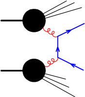
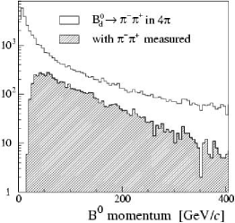
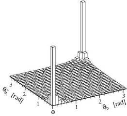
(a)Typical diagram for $b\overline{b}$ production in pp collisions [17].	(b) Momentum distribution for ${\rm B_{d}^{0}}$ mesons in ${\rm{\rm B_{d}^{0}}\to\pi^{+}\pi^{-}}$ decays [12].	(c) Polar angles of hadrons formed from $b\overline{b}$ pairs, calculated by PYTHIA [12].

Figure 3: B–hadrons at LHCb.

3.2 Luminosity at the LHCb interaction point

At the LHC design luminosity, each bunch crossing would involve many inelastic proton–proton interaction. Such multiple interactions severely complicate the task of ${\rm B^{0}}$–tagging, and of cleanly locating the primary and secondary vertices.

Therefore the luminosity at the LHCb detector is reduced to $\mathrm{2\cdot 10^{32}\,cm^{-1}s^{-1}}$ by defocussing the beam at the LHCb interaction point. Apart from optimising the number of single interactions, also the trigger performance, detector occupancy and radiation levels are taken into account when choosing the design luminosity. Remaining multiple interactions are identified by the Pile-Up system. While LHCb is optimised for single interactions, remaining multiple interactions are not necessarily discarded. The decision whether to keep of discard a multiple interaction event is made at trigger Level-0.

With this luminosity, LHCb expects about $10^{12}$ $b\overline{b}$ events per year. Due to its comparably moderate luminosity requirements, LHCb can start its full physics programme from the first day of LHC running.

3.3 The LHCb detector

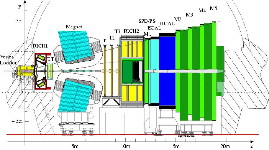
Figure 4: The LHCb Detector

LHCb is specifically designed to make best use of the large number of $b\overline{b}$ pairs produced at the LHC. The LHCb detector is a single arm spectrometer with an angular acceptance from an outer limit of $\mathrm{250\,mrad}$ in the non-bending plane, and $\mathrm{300\,mrad}$ in the bending plane, down $\mathrm{15\,mrad}$. This geometry is motivated by the kinematics of $b\overline{b}$ production in high energy proton–proton collisions, as discussed above.

Amongst the most important features of the the LHCb detector are:

• Acceptance down to small polar angles / large pseudo-rapidity, to maximise B-hadron yield.

• Excellent proper time resolution to exploit the full ${\rm B}$ physics potential at the LHC, including measurements in the rapidly oscillating ${\rm B_{s}^{0}}$ system.

• Particle identification by two Ring Imaging CHerenkov (RICH) counters, for clean data samples and flavour tagging with Kaons.

• Dedicated ${\rm B}$ trigger, including high $\mathrm{p_{t}}$ hadron and lifetime triggers for high efficiency.

Figure 4 shows a schematic overview of the LHCb detector. It comprises a vertex detector system, which includes the pile–up veto counter; a magnet and a tracking system; two RICH counters; an electromagnetic calorimeter and a hadron calorimeter, and a muon detector. All detector sub–systems, except for RICH 1, are split into two halves that can be separated horizontally for maintenance and access to the beam pipe.

3.3.1 Material Budget

LHCb has recently undergone a major re-optimisation [3], which led to a substantially reduced material budget. Particular weight reduction has been achieved in the following subsystems:

• Beam pipe: Now made from Be or Al/Be alloy.

• Vertex Detector: 21, $\mathrm{220\,\mu m}$ thin detector elements.

• RICH: Mirrors are now to be made from light materials (either Carbon fibre or Beryllium), support structures have been moved outside the acceptance.

• Tracking: All tracking stations inside the magnet have been removed. There is 1 (double) station before, and 3 stations behind magnet.

The resulting material “seen” by a particle before RICH 1 is typically $40\%$ of a radiation length, and $12\%$ of an interaction length.

3.4 Magnet

To achieve a precision on momentum measurements of better than half a percent for momenta up to $\mathrm{200\,GeV}$, the LHCb dipole provides integrated field of $\mathrm{4\,Tm}$. As seen in figure 4, the magnet poles are inclined to follow the LHCb acceptance angles. This allows the $\mathrm{4\,Tm}$ to be retained with a power consumption of $\mathrm{4.2\,MW}$. The warm magnet design chosen of LHCb allows for regular field inversions to reduce systematic errors in CP violation measurements. The LHCb magnet is currently being installed in the collision hall.

3.5 Tracking

The LHCb tracking system consists of the Vertex Locator (VELO), one tracking station before the magnet (“Trigger Tracker”), and three tracking stations behind the magnet (T1 - T3). The VELO, the Trigger Tracker, and high-occupancy regions in T1-T3 near the beam line (“Inner Tracker”) use Si technology, while the outer regions in T1-T3 (“Outer Tracker”) use straw tube drift chambers.

3.5.1 The Vertex Locator

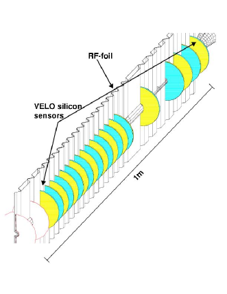
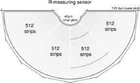
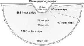
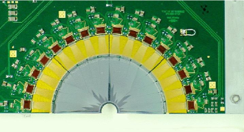
(a) VELO with RF-foil, 21 $r-\phi$ detector stations, and two upstream $r$ stations for the Pile Up system.	(b) $r$ and $\phi$ sensors. For each sensor, 2 readout strips are indicated by dotted lines, for illustration.	(c) Prototype Si sensor with readout electronics

Figure 5: The LHCb Vertex Locator (VELO)

To measure the time dependent decay rate asymmetries, a detector with excellent spatial resolution is required, especially for measurements in the rapidly oscillating ${\rm B_{s}^{0}}$ system. At LHCb, this is provided by the Vertex Locator (VELO, Fig 5), comprising a series of 21 detector station placed along the beam line covering a distance of about $\mathrm{1\,m}$. Each station consists of two pairs of half-circular Si microstrip detectors (Fig 5), one pair measuring the radial ($r$), and one the azimuthal ($\phi$) co-ordinate. The sensors are made from $\mathrm{220\,\mu m}$ thin Silicon, and have a readout pitch between $\mathrm{37\,\mu m}$ and $\mathrm{102\,\mu m}$. To achieve the required high acceptance at small polar angles (see section 3.1), the sensitive area starts at only $\mathrm{8\,mm}$ from the beam line. To protect the detectors during beam injection, they can be retracted from the beam line. To minimise the material between the interaction region and the detector, the Si sensors are placed inside a secondary vacuum, separated from the primary vacuum by a $\mathrm{\sim\frac{1}{4}\,mm}$ thin Al foil, which also shields the sensors from RF pickup from the beam. In addition to the 21 VELO stations which are mostly “downstream” of the interaction point (between the interaction point and the rest of the detector), there are two $r$-disks upstream of the interaction point which make up the Pile-Up System, used in the trigger Level-0 for identifying multiple interaction events. The VELO provides an impact parameter resolution of $\sigma_{IP}=\mathrm{14\,\mu m}+\frac{\mathrm{35\,\mu m}}{\mathrm{p_{T}/GeV}}$ and a time resolution of $\sigma_{tau}\sim\mathrm{40\,ps}$ (for ${\rm{\rm B_{s}^{0}}\to D_{s}\pi}$), sufficient to resolve ${\rm{\rm B_{s}^{0}}}$ oscillations up to $\Delta m_{s}=\mathrm{68\,ps^{-1}}$ corresponding to $x_{s}=105$.

3.5.2 Tracking

Each tracking station consists of 4 layers. The outer layers (1 and 4) measure the track coordinate in the bending plane (“$x$-layers”). The inner layers (2 and 3) are rotated by $\mathrm{+5^{\circ}}$ and $\mathrm{-5^{\circ}}$ respectively relative to the $x$-layers (“stereo layers”). This geometry optimises the resolution in the bending plane, for precise momentum measurements, while providing sufficient resolution in the non-bending plane for effective 3-D pattern recognition.

The 4 layers of the Trigger Tracker are split into two sub stations, separated by $\mathrm{30\,cm}$. This allows a rough momentum estimation from the bending of the tracks in the magnetic fringe field. This momentum information is used in the trigger Level-1 decision. The Si detectors in the Trigger Tracker and Inner Tracker have a read out pitch of $\mathrm{198\,\mu}$, with strip lenghs of up to $\mathrm{33\,cm}$ in the Trigger Tracker, and $\mathrm{11-22\,cm}$ in the Inner Tracker. The thickness of Si layers is $\mathrm{320\,\mu}$ for the Inner Tracker, and $\mathrm{500\,\mu m}$ for the Trigger Tracker. The Outer Tracker is made of $\mathrm{5\,mm}\times\mathrm{4.7\,m}$ straw tubes, with a fast drift gas ($75\%\mathrm{Ar}$, $15\%\mathrm{CF_{4}}$, $10\%\mathrm{CO_{2}}$), allowing signal collection in less than $\mathrm{50\,ns}$. The LHCb tracking system provides a momentum resolution of $\frac{\delta p}{p}=0.37\%$. For the example of ${\rm B_{s}\to D_{s}K}$, this translates into a mass resolution of $\mathrm{14\,MeV}$. The track-finding efficiency is $94\%$ for tracks with hits in all tracking stations. The Ghost rate is $9\%$ ($3\%$ for tracks with $p_{T}>\mathrm{0.5\,GeV}$).

3.6 Calorimetry

The main design constraints for the calorimeter system come from its central role in the Level-0 trigger decision, which must be provided and processed within the $\mathrm{25\,ns}$ between each bunch crossing. The general structure of the calorimeter system is as follows: the first element seen by a particle coming from the interaction point is a scintillator pad detector (SPD), that signals charged particles. This is followed by a $\mathrm{12\,mm}$ lead wall and another SPD, which together form the preshower detector (PS). This is then followed by $25$ radiation lengths ($1.1$ interaction lengths) of a $\mathrm{Pb}$/scintillator Shashlik calorimeter (ECAL) and $5.6$ interaction length of a iron/scintillator tile hadron calorimeter (HCAL).

Most ECAL modules, and a large fraction of HCAL modules have already been delivered to CERN. In testbeams an energy resolution of

$$\left(\frac{\sigma_{E}}{E}\right)_{\mathrm{ECAL}}=\frac{9.4\%}{\sqrt{\mathrm{E\,/GeV}}}\oplus 0.83\%\oplus\frac{\mathrm{0.145\,GeV}}{E},\;\;\;\;\;\;\left(\frac{\sigma_{E}}{E}\right)_{\mathrm{HCAL}}=\frac{75\%}{\sqrt{\mathrm{E\,/GeV}}}\oplus 10\%$$

has been achieved.

3.7 Muon System

The muon system provides offline muon identification, and information for the trigger Level-0. It consists of four stations behind the calorimeters (M2-M5), and one unshielded station in front of the calorimeters (M1). Most of the muon chambers will be Multi-Wire Proportional Chambers (MWPC). For the central region of M1 ($\mathrm{0.6\,m^{2}}$), triple GEM technology will be more suitable due the expected high rates in that area.

3.8 RICH

LHCb intends to perform high precision measurements in many different ${\rm B}$ decay channels. Many interesting decay channels are themselves backgrounds to topologically similar ones. Typically the branching ratios are of the order of $\sim 10^{-5}$. The particle identification and in particular ${\rm K/\pi}$ separation provided by the RICH is essential for obtaining the clean samples needed to perform a comprehensive range of high–precision $\mathcal{CP}$ violation measurements, and allows the use of Kaons of flavour tagging, dramatically improving the tagging performance at LHCb 3.10.

RICH 1	Rings in RICH 1	RICH 2 (with	Rings in RICH 2
		RICH 1 for scale)

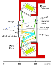
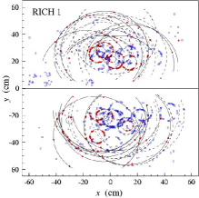
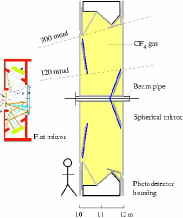
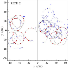
Figure 6: The LHCb RICH system used 2 detectors and 3 radiators, to provide ${\rm K-\pi}$ separation from $\mathrm{\sim 1\,GeV}$ to beyond $\mathrm{100\,GeV}$. The figure shows RICH 1 and RICH 2 with the respective event displays for a typical event. The points represent the detector response. The rings drawn through the points are the result of a global pattern recognition algorithm, which uses the tracking results as a seed.

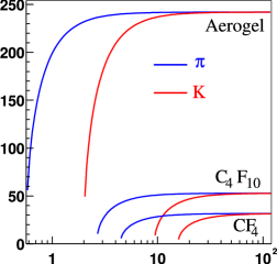
(a) Momenta of tracks in ${\rm B\to\pi\pi}$ events, and tagging Kaons. For both, ${\rm K/\pi}$ separation is essential.	(b) Cherenkov angle $\theta_{C}$ vs momentum for Kaons an pions for each radiator in the LHCb RICH.	(c) Polar angle $\theta$ vs momentum for all tracks in $B_{d}^{0}\to\pi\pi$ evts, approx. RICH-coverage indicated.
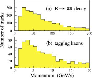
	$\theta_{C}$ $\mathrm{[mrad]}$ $p$ $\mathrm{[GeV]}$

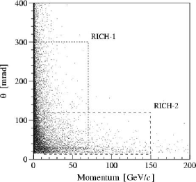
Figure 7: The LHCb RICH employs 3 Radiators in 2 RICH detectors to provide ${\rm K/\pi}$ separation from $\mathrm{\sim 1\,GeV}$ to beyond $\mathrm{100\,GeV}$.

Figure 7 (a) shows the momentum distribution of (a) pions in ${\rm{\rm B_{d}^{0}}\to{\rm\pi^{+}}{\rm\pi^{-}}}$ events, and (b) tagging Kaons. This illustrates the need for ${\rm K/\pi}$ separation over a wide range of momenta; LHCb seeks ${\rm K/\pi}$ separation from momenta of $\mathrm{\sim 1\,GeV}$ to beyond $\mathrm{100\,GeV}$.

RICH (Ring Imaging CHerenkov) counters measure the opening angle $\theta_{C}$ of the Cherenkov cone emitted by particles as they traverse a transparent medium, by imaging it onto an array of photo detectors as illustrated in Fig 6. This opening angle depends on the speed of the particle. Combining it with the momentum information from the tracking system, allows to identify the particle by its mass. To cover a momentum range from $\mathrm{\sim 1\,GeV}$ to beyond $\mathrm{100\,GeV}$, LHCb employs two RICH detectors and three radiators, Aerogel ($n=1.03$) and $\mathrm{C_{4}F_{10}}$ gas ($n=1.0014$) in RICH 1 and $\mathrm{CF_{4}}$ gas ($n=1.0005$) in RICH 2. The angular and approximate momentum coverage of the two RICH detectors at LHCb is shown in 7, superimposed over a scatter plot showing polar angles and momenta of particles in ${\rm B_{d}\to\pi\pi}$ events.

(b) Inv. mass of ${\rm B_{s}\to D_{s}K}$    with ${\rm B_{s}\to D_{s}\pi}$ background
	without RICH	with RICH

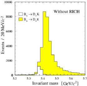
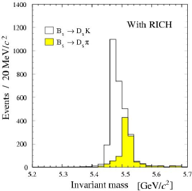
Figure 8: Without RICH particle ID, many decays would be swamped by topologically similar background. Illustrated here for the $\gamma$-sensitive channel ${\rm B_{s}\to D_{s}K}$, which has a $\sim 10$ times smaller B.R. than its dominant background, ${\rm B_{s}\to D_{s}\pi}$.

Figure 8 illustrates how the RICH particle ID cleans up the ${\rm B_{s}\to D_{s}K}$ signal, a $\gamma$-sensitive channel that would otherwise be completely dominated by background from ${\rm B_{s}\to D_{s}\pi}$ which has a $\sim 10$ times higher branching fraction.

3.9 LHCb Trigger

The LHCb trigger has the task of reducing the event rate of $\mathrm{40\,MHz}$ by a factor of $200,000$ to the write-to-tape rate of $\mathrm{200\,Hz}$, while keeping as many interesting B-events as possible. This is achieved in three steps.

• Level-0 uses information from the Pile-Up detector, the Calorimeters and the Muon Chambers, to reduce the event rate from $\mathrm{40\,MHz}$ to $\mathrm{1\,MHz}$.

• Level-1  uses momentum and impact parameter information from the VELO and the Trigger Tracker, to reduce the event rate further to $\mathrm{40\,kHz}$.

• The High Level Trigger (HLT) will have access to the complete event information to perform full event reconstruction.

While the Level-0 algorithm will run on dedicated hardware, Level-1 and the HLT will run trigger software on computing farms built from off-the-shelf components.

3.10 Flavour Tagging

To measure the time dependent decay rate asymmetries from which the CKM phases are extracted, the flavour of the reconstructed B meson at the time of creation needs to be known. Usually, this is done by looking at B decay products from the opposite-side B-hadron created alongside the one being reconstructed. (“lepton tag”, “Kaon tag”, “Vertex Charge”).

An alternative strategy is same side tagging, which uses the correlation between the flavour of a ${\rm B_{s}}$ meson and the charge of a ${\rm K^{+}}$ picking up the 2$\mathrm{\mbox{}^{nd}}$ $s$ quark produced in the process. In principle, this method also works with ${\rm B_{d}}$ mesons and pions, but given the large number of pions created in a hadron collider, it is much more difficult to pick out the right one.

Tag $\varepsilon$ $\omega$ $\varepsilon_{\mathrm{eff}}$ ${\rm\mu}$ 11% 35% 1% ${\rm e}$ 5% 36% 0.4% ${\rm K_{\mathrm{opp-side}}}$ 17% 31% 2.4% $Q_{\mathrm{Vtx}}$ 14% 40% 1% ${\rm B^{0}_{d}}$ all 41% 35% 4% ${\rm K_{\mathrm{same-side}}}$ 18% 33% 2.1% ${\rm B^{0}_{s}}$ all 50% 33% 6%

The figure of merit for the tagging performance is given by the “effective tagging efficiency” $\varepsilon_{\mathrm{eff}}$ (also known as $\epsilon D^{2}$): $\varepsilon_{\mathrm{eff}}=\varepsilon\left(1-\omega\right)^{2}$ The statistical significance of $N$ events with an effective tagging efficiency $\varepsilon_{\mathrm{eff}}$ is equivalent to $\varepsilon_{\mathrm{eff}}N$ perfectly tagged events.

Table 1: Tagging efficiencies ($\varepsilon$), wrong-tag fractions ($\omega$) and effective tagging efficiencies $\varepsilon_{\mathrm{eff}}\equiv\varepsilon(1-2\omega)^{2}$ for ${\rm B\to hh}$.

Table 1 shows the expected tagging performance at LHCb for ${\rm B\to\pi\pi}$ and ${\rm B_{s}\to KK}$.

4 Physics

By the year 2007, we expect a very precise measurement of the angle $\beta$, from the B-factories and the Tevatron, and results for the mass and lifetime difference of the CP eigenstates of the ${\rm B_{s}}$ system, $\Delta m_{s}$ and $\Delta\Gamma_{s}$ from the Tevatron. With its huge number of $b\overline{b}$ pairs, LHCb will be able to significantly improve the precision on all of these measurements within the first year of data taking. However, here we focus on one of the most exciting Physics prospects at LHCb, the experiment’s ability to perform precision measurements of the angle $\gamma$ in many different decay channels both in the ${\rm B_{d}}$ and ${\rm B_{s}}$ system. Both, the B-factories and CDF expect some measurement of $\gamma$ by 2007, but this is unlikely to be precise enough to provide a significant constraint on the Unitarity Triangle. LHCb will measure $\gamma$ in many different channels, some more and some less susceptible to New Physics, with a typical precision of $\mathrm{5^{\circ}}-\mathrm{15^{\circ}}$ for each channel after one year of data taking. We will demonstrate on three examples different strategies of measuring $\gamma$ at LHCb.

4.1 ${\rm B_{d}\to\pi\pi}$ and ${\rm B_{s}\to KK}$

4.1.1 Principle

If there were only the tree contribution…	${\rm B^{0}_{d}\to\pi\pi}$ would measure $2(\beta+\gamma)$…	… but there are Penguins:

Figure 9: The phase difference between ${\rm B_{d}\to\pi^{+}\pi^{-}}$ and ${\rm B_{d}\to\bar{B}_{d}\to\pi^{+}\pi^{-}}$ is affected by both tree and penguin contributions. These can be disentangled by simultaneously analysing the U-Spin related decay ${\rm B_{s}\to KK}$.

The decay ${\rm B_{d}\to\pi\pi}$ is, due to the $b\to u$ transition in the tree diagram in figure 9, sensitive to the CKM angle $\gamma$. However, the presence of penguin contributions severely complicates the interpretation of the observed CP asymmetries in terms of CKM angles. At the same time, penguin diagrams are interesting, because they are sensitive to New Physics. A possible strategy that allows the tree and penguin contributions to be disentangled, and thus measure $\gamma$, is due to Fleischer [19], and uses U-spin symmetry of the strong interaction to relate observables in ${\rm B\to\pi\pi}$ and ${\rm B_{s}toKK}$. The time dependent decay rate asymmetry can be parametrised as

$$\frac{\Gamma\left({\rm B_{d}\to\pi^{+}\pi^{-}}\right)-\Gamma\left({\rm\bar{B}_{d}\to\pi^{+}\pi^{-}}\right)}{\Gamma\left({\rm B_{d}\to\pi^{+}\pi^{-}}\right)+\Gamma\left({\rm\bar{B}_{d}\to\pi^{+}\pi^{-}}\right)}=A_{{\rm\pi\pi}}^{\mathrm{Dir}}\cos(\Delta m_{d}\tau)+A_{{\rm\pi\pi}}^{\mathrm{Mix}}\sin(\Delta m_{d}\tau),$$ (11)

and similarly for ${\rm B_{s}\to KK}$. This provides four observables: $A_{{\rm\pi\pi}}^{\mathrm{Dir}}$, $A_{{\rm\pi\pi}}^{\mathrm{Mix}}$, $A_{{\rm KK}}^{\mathrm{Dir}}$, and $A_{{\rm KK}}^{\mathrm{Mix}}$. These can be parametrised with the following seven parameters:

• $d,\theta$ hadronic parameters describing “penguin-to-tree” ratio and phase in ${\rm B_{d}}$.

• $d^{\prime},\theta^{\prime}$ hadronic parameters related to “penguin-to-tree” ratio and phase for ${\rm B_{s}}$.

• $\phi_{d}$ = ${\rm B_{d}}$ mixing phase, $2\beta$ in SM.

• $\phi_{s}$ = ${\rm B_{s}}$ mixing phase, $2\delta\gamma\approx 0$ in SM.

• $\gamma$ is what we want to measure.

These can be reduced to three parameters, as follows

• $2\beta$ and $2\delta\gamma$ will be known precisely from ${\rm B\to J/\!\psi K_{s}}$ and ${\rm B_{s}\to J/\!\psi\phi}$

• $d,\theta,d^{\prime},\theta^{\prime}$ depend on the strong interaction only. Assuming U-spin symmetry, we set $d=d^{\prime}$ and $\theta=\theta^{\prime}$.

Further details can be found in [19].

Channel	# evts	B/S	tagging	mistag
	per year		eff	frac
${\rm B\to\pi\pi}$	$\mathrm{26\,k}$	$<0.7$	$41.8\%$	$34.9\%$
${\rm B_{s}\to KK}$	$\mathrm{37\,k}$	$<0.5$	$49.8\%$	$33.0\%$

Table 2: Expected reconstruction and tagging performance for ${\rm B\to\pi\pi}$ and ${\rm B_{s}\to KK}$.

$\Delta m_{s}$	15	20	25	30
$\sigma(\gamma)$	4.0	4.9	5.9	8.5
$\frac{\Delta\Gamma_{s}}{\Gamma_{s}}$	0	0.1	0.2
$\sigma(\gamma)$	5.2	4.9	4.5
$\gamma$	55	65	75	85	95	105
$\sigma(\gamma)$	5.8	4.9	4.3	4.7	4.7	4.7
$\vartheta$	120	140	160	180	200
$\sigma(\gamma)$	3.8	3.8	4.9	6.7	5.2
$d$	0.1	0.2	0.3	0.4
$\sigma(\gamma)$	1.8	2.7	4.9	9.0
$2\delta\gamma$	0	$-0.04$	$-0.1$	$-0.2$
$\sigma(\gamma)$	4.9	4.9	4.9	5.4

Table 3: Statistical uncertainty on $\gamma$ for one year of data. Unless otherwise specified, $\Delta m_{s}=20\mathrm{ps^{-1}}$, $\frac{\Delta\Gamma_{s}}{\Gamma_{s}}=0.1$, $\gamma=65^{\circ}$, $\vartheta=160^{\circ}$, $d=0.3$, $2\delta\gamma=-0.04$. $\Delta m_{s}$ values are given in $\mathrm{ps^{-1}}$, $2\delta\gamma$ values in radians, while $\gamma$, $\vartheta$ and $\sigma(\gamma)$ are given in degrees.

The expected event yields and tagging performance for ${\rm B\to\pi\pi}$ and ${\rm B_{s}\to KK}$ are given in table 2. LHCb relies heavily on its ${\rm K/\pi}$ separation capabilities to achieve the required sample purity, as otherwise the different hadronic two body decay modes of B hadrons are virtually indistinguishable.

The statistical precision on $\gamma$ that can be achieved with reconstruction and tagging performance depends on various parameters, especially the “penguin over tree ratio”, $d$, and the rapidity of ${\rm B_{s}}$ oscillations, given by the mass difference $\Delta m_{s}$. For a typical parameter set the precision on $\gamma$ is $\sim\mathrm{5^{\circ}}$. Statistical uncertainties on $\gamma$ for various sets of parameters are given in table 3.

4.2 ${\rm B_{s}\to D_{s}K}$

An alternative way to tackle the problem of penguin contributions is to look at decays that don’t have any, like ${\rm B_{s}\to D_{s}K}$, or ${\rm B_{d}\to D^{(*)}\pi}$ [20]. These decays are expected to be rather insensitive to New Physics contributions, and therefore measure a “Standard Model $\gamma$”, providing a benchmark that other decays, that are more sensitive to New Physics, can be compared against. Since the final state is not a CP eigenstate, two CP-conjugate asymmetries need to be measured,

$$A(\tau)=\frac{\Gamma\left({\rm B_{s}\to D_{s}^{-}K^{+}}\right)-\Gamma\left({\rm\bar{B}_{s}\to D_{s}^{-}K^{+}}\right)}{\Gamma\left({\rm B_{s}\to D_{s}^{-}K^{+}}\right)+\Gamma\left({\rm\bar{B}_{s}\to D_{s}^{-}K^{+}}\right)}\;,\;\;\bar{A}(\tau)=\frac{\Gamma\left({\rm\bar{B}_{s}\to D_{s}^{+}K^{-}}\right)-\Gamma\left({\rm B_{s}\to D_{s}^{+}K^{-}}\right)}{\Gamma\left({\rm\bar{B}_{s}\to D_{s}^{+}K^{-}}\right)+\Gamma\left({\rm B_{s}\to D_{s}^{+}K^{-}}\right)}$$

The CP violating effect is in the difference between those asymmetries. This measurement is sensitive to $2\delta\gamma+\gamma$, and a possible strong phase difference $\Delta_{\mathrm{T1/T2}}$. Further details are given in [20].

$\Delta m_{s}$	15	20	25	30
$\sigma(2\delta\gamma+\gamma)$	12.1	14.2	16.2	18.3
$\frac{\Delta\Gamma_{s}}{\Gamma_{s}}$	0	0.1	0.2
$\sigma(2\delta\gamma+\gamma)$	14.7	14.2	12.9
$2\delta\gamma+\gamma$	55	65	75	85	95	105
$\sigma(2\delta\gamma+\gamma)$	14.5	14.2	15.0	15.0	15.1	15.2
$\Delta_{\mathrm{T1/T2}}$	$-20$	$-10$	0	$+10$	$+20$
$\sigma(2\delta\gamma+\gamma)$	13.9	14.1	14.2	14.5	14.6

Table 4: Expected statistical uncertainty on $2\delta\gamma+\gamma$ for one year of data. Unless otherwise specified, $\Delta m_{s}=20\mathrm{ps^{-1}}$, $\frac{\Delta\Gamma_{s}}{\Gamma_{s}}=0.1$, $2\delta\gamma+\gamma=\mathrm{65^{\circ}}$ and $\Delta_{\mathrm{T1/T2}}=\mathrm{0^{\circ}}$. All values are given in degrees, except $\Delta m_{s}$ in $\mathrm{ps^{-1}}$.

The particle ID capabilities of LHCb are crucial for the reconstruction of this decay, that would otherwise be swamped by background from ${\rm B_{s}\to D_{s}^{-}\pi^{+}}$, which has a $\sim 10$ times higher branching ratio. LHCb expects to reconstruct $\mathrm{5.4\,k}$ ${\rm B_{s}\to D^{-}K^{+}}$ events per year with a background-to-signal of better than $0.5$. This translates into a sensitivity on $\gamma$ of typically $\mathrm{\sim 15^{\circ}}$, depending on other parameters, especially $\Delta m_{s}$. Results for different parameters sets are given in Table 4.

4.3 $\gamma$ with ${\rm B_{d}^{0}\to\bar{D}^{0}K^{*0}}$ ${\rm B_{d}^{0}\to D^{0}_{\mathrm{CP}}K^{*0}}$

The decay ${\rm B_{d}^{0}\to\bar{D}^{0}K^{*0}}$ offers the possibility of measuring $\gamma$, using untagged, time-integrated samples [21]. This method is sensitive to New Physics in ${\rm D^{0}}$ oscillations. The following 6 parameters are measured:
$\displaystyle\Gamma_{+}$ $\displaystyle=$ $\displaystyle\Gamma\left({\rm B^{0}\to D^{0}(\pi^{+}K^{-})K^{*0}}\right)$ $\displaystyle\Gamma_{-}$ $\displaystyle=$ $\displaystyle\Gamma\left({\rm B^{0}\to\bar{D}^{0}(K^{+}\pi^{-})K^{*0}}\right)$ $\displaystyle\Gamma_{\mathrm{CP}}$ $\displaystyle=$ $\displaystyle\Gamma\left({\rm B^{0}\to D^{0}_{\mathrm{CP}}(K^{+}K^{-})K^{*0}}\right)$ $\displaystyle\bar{\Gamma}_{+}$ $\displaystyle=$ $\displaystyle\Gamma\left({\rm\bar{B}^{0}\to{D}^{0}(\pi^{+}K^{-})\bar{K}^{*0}}\right)$ $\displaystyle\bar{\Gamma}_{-}$ $\displaystyle=$ $\displaystyle\Gamma\left({\rm\bar{B}^{0}\to\bar{D}^{0}(K^{+}\pi^{-})\bar{K}^{*0}}\right)$ $\displaystyle\bar{\Gamma}_{\mathrm{CP}}$ $\displaystyle=$ $\displaystyle\Gamma\left({\rm B^{0}\to D^{0}_{\mathrm{CP}}(K^{+}K^{-})\bar{K}^{*0}}\right)$

They are related as follows:

$${\Gamma_{+}=\bar{\Gamma}_{-}\equiv g_{1}},\;\;\;{\Gamma_{-}=\bar{\Gamma}_{+}\equiv g_{2}}$$ (12)

and

$$\Gamma_{\mathrm{CP}}=\frac{{g_{1}}+{g_{2}}}{2}+\sqrt{{g_{1}}{g_{2}}}\cos\left(\Delta+\gamma\right)\;,\;\;\bar{\Gamma}_{\mathrm{CP}}=\frac{{g_{1}}+{g_{2}}}{2}+\sqrt{{g_{1}}{g_{2}}}\cos\left(\Delta-\gamma\right)$$ (13)

Where $\Delta$ is a possible strong phase difference.

$\gamma$	$55^{\circ}$	$65^{\circ}$	$75^{\circ}$	$85^{\circ}$	$95^{\circ}$	$105^{\circ}$
$\sigma(\gamma)$	$9.0^{\circ}$	$8.2^{\circ}$	$7.6^{\circ}$	$7.1^{\circ}$	$7.0^{\circ}$	$7.0^{\circ}$

Table 5: Expected statistical precision on $\gamma$ for different values of $\gamma$ after one year of data taking. The value of $\Delta$ is set to $0$.

LHCb expects within $1$ year of data taking to reconstruct $\mathrm{3.6\,k}$ events to measure $\Gamma_{-},\bar{\Gamma}_{-}$, $\mathrm{0.49\,k}$ events to measure $\Gamma_{+},\bar{\Gamma}_{+}$, and $\mathrm{0.31\,k}$ events to measure $\Gamma_{\mathrm{CP}},\bar{\Gamma}_{\mathrm{CP}}$. Mainly because no tagging is required, the statistical weight of each reconstructed decay is much higher than in measurements using time-dependent decay rate asymmetries. Therefore, despite the comparably small data sample, a very competitive precision on $\gamma$ of $\sigma(\gamma)=\mathrm{8.2^{\circ}}$ (for $\gamma=\mathrm{65^{\circ}},\Delta=0$) after one year can be achieved. Results for different values of $\gamma$ are given in table 5.

5 Summary

Channel Standard New Model Physics ${\rm B_{d}^{0}\to D^{(*)\pm}\pi^{\mp}}$ $\mathbf{\surd}$ ${\rm B_{s}^{0}\to D_{s}^{\pm}K^{\mp}}$ $\mathbf{\surd}$ $\parbox{73.97733pt}{ ${\rm B_{d}^{0}\to\pi^{+}\pi^{-}}$\\ ${\rm B_{s}^{0}\to K^{+}K^{-}}$}\;\Bigg{\}}$ $\mathbf{\surd}$ $\parbox{73.97733pt}{ ${\rm B_{d}^{0}\to\bar{D}^{0}K^{*0}}$ ${\rm B_{d}^{0}\to D^{0}_{\mathrm{CP}}K^{*0}}$}\;\Bigg{\}}$ $\mathbf{\surd}$

Typical precision in each channel $\mathrm{\sim 5^{\circ}}-\mathrm{15^{\circ}}$ after 1 year. More channels are under investigation, e.g.: $\parbox{73.97733pt}{ ${\rm B_{d}^{0}\to D_{d}^{+}D_{d}^{-}}$ ${\rm B_{s}^{0}\to D_{s}^{+}D_{s}^{-}}$}\;\Bigg{\}}$ which is highly sensitive to New Physics, since $\gamma$ enters via penguins only [22]. (${\rm B_{s}^{0}\to D_{s}^{+}D_{s}^{-}}$ is also sensitive to $\frac{\Delta\Gamma_{s}}{\Gamma_{s}}$, and $\delta\gamma$).

Table 6: Some $\gamma$ sensitive channels accessible at LHCb. It is indicated if the channels are expected to be sensitive to New Physics, or to the Standard Model $\gamma$.

The recently re-optimised LHCb detector [3] is on track for data taking in 2007. The detector is designed to make best use of the vast number of B hadrons of all flavours, that are expected at the LHC. LHCb has a comprehensive programme of high-precision B physics, including competitive measurements of the CKM phases $\beta,\gamma$, and mass and lifetime difference in the ${\rm B_{s}}$ system within the first year of data taking. The physics programme also includes higher order effects (e.g. $\delta\gamma$), rare B decays, and many more.

In this report we focused on one of the most exciting prospects at LHCb, the possibility to perform precision measurements of the angle $\gamma$ in many different decay channels in both the ${\rm B_{d}}$ and ${\rm B_{s}}$ system. Some of the measurements will be more and some less sensitive to New Physics contributions. A selection of such channels are listed in Table 6. The typical resolution in $\gamma$ is $\mathrm{5^{\circ}}-\mathrm{15^{\circ}}$ for each channel, within a single year of data taking. This will thoroughly over constrain the Standard Model description of CP violation, providing important Standard Model measurements with a high sensitivity to New Physics.

References

- [1] LHCb Technical Design Report, http://lhcb.web.cern.ch/lhcb/TDR/TDR.htm, comprising [2], [3], [4], [5], [6], [8], [9], [10], [11].
- [2] LHCb TDR 10 Trigger System, September 2003. CERN-LHCC-2003-031
- [3] LHCb TDR 9 Reoptimised Detector - Design and Performance, September 2003. CERN-LHCC-2003-030
- [4] LHCb TDR 8 Inner Tracker, November 2002. CERN-LHCC-2002-029
- [5] LHCb TDR 7 Online System, December 2001. CERN-LHCC-2001-040
- [6] LHCb TDR 6 Outer Tracker, September 2001. CERN-LHCC-2001-024
- [7] LHCb TDR 5 VELO, May 2001. CERN-LHCC-2001-011
- [8] LHCb TDR 4 Muon System, May 2001. CERN-LHCC-2001-010, and Addendum to TDR 4, January 2003, CERN-LHCC-2003-002
- [9] LHCb TDR 3 RICH, September 2000. CERN-LHCC-2000-037
- [10] LHCb TDR 2 Calorimeters, September 2000. CERN-LHCC-2000-036
- [11] LHCb TDR 1 Magnet, Jan 2000. CERN-LHCC-2000-007
- [12] LHCb Technical Proposal, February 1998. CERN/LHCC/98-4.
- [13] H. H cker, H. Lacker, S. Laplace and F. Le Diberder Eur. Phys. J. C21, 225-259 (2001) LAL 06/01 [hep-ph/0104062] http://www.slac.stanford.edu/xorg/ckmfitter/ckm_wellcome.html
-
[14]
Heavy Flavour Averaging Group.
Method: ALEPH, CDF, DELPHI, L3, OPAL, SLD
, June 2001, CERN-EP/2001-050, arXiv:hep-ex/0112028.
Results Winter 2004: http://www.slac.stanford.edu/xorg/hfag/triangle/winter2004/index.shtml - [15] A. J. Buras, M. E. Lautenbacher and G. Ostermaier, Phys. Rev. D 50 (1994) 3433 [arXiv:hep-ph/9403384].
- [16] L. Wolfenstein, Phys. Rev. Lett. 51 (1983) 1945.
- [17] P. Nason et al. Bottom production. In G. G. Altarelli and M. L. Mangano, editors, 1999 CERN Workshop on Standard Model Physics (and more) at the LHC, CERN, Geneva, Switzerland, 25 - 26 May 1999: Proceedings, 2000. CERN-2000-004.
- [18] LHC - challenges in accelerator physics. http://lhc.web.cern.ch/lhc/general/gen_info.htm status: January 14, 1999.
- [19] R. Fleischer, Phys. Lett. B 459 (1999) 306 [arXiv:hep-ph/9903456].
- [20] R. Aleksan, I. Dunietz and B. Kayser, Z. Phys. C 54 (1992) 653.
- [21] I. Dunietz, Phys. Lett. B 270 (1991) 75.
- [22] R. Fleischer, Eur. Phys. J. C 10 (1999) 299 [arXiv:hep-ph/9903455].