DESY 04-240 ISSN 0418-9833

December 2004

A Direct Search for Stable Magnetic Monopoles Produced in Positron-Proton Collisions at HERA
H1 Collaboration

A direct search has been made for magnetic monopoles produced in $e^{+}p$ collisions at a centre of mass energy of 300 GeV at HERA. The beam pipe surrounding the interaction region in 1995-1997 was investigated using a SQUID magnetometer to look for stopped magnetic monopoles. During this time an integrated luminosity of 62 pb^-1 was delivered. No magnetic monopoles were observed and charge and mass dependent upper limits on the $e^{+}p$ production cross section are set.

(Submitted to European Physical Journal C)

1 Introduction

One of the outstanding issues in modern physics is the question of the existence of magnetic monopoles. Dirac showed that their existence leads naturally to an explanation of electric charge quantisation[1]. Magnetic monopoles are also predicted from field theories which unify the fundamental forces[4, 5, 2, 3]. Furthermore, the formation of a monopole condensate provides a possible mechanism for quark confinement[6]. Nevertheless, despite a large number of searches[7, 8] using a variety of experimental techniques, no reproducible evidence has been found to support the existence of monopoles. Searches for magnetic monopoles produced in high energy particle collisions have been made in $p\bar{p}$[9, 10, 11] and $e^{+}e^{-}$[12, 13, 14, 15, 16, 17] interactions. This paper describes the first search for monopoles produced in high energy $e^{+}p$ collisions.

The quantisation of the angular momentum of a system of an electron with electric charge $e$ and a monopole with magnetic charge $g$ leads to Dirac’s celebrated charge quantisation condition $eg=n\hslash c/2$, where $\hslash$ is Planck’s constant divided by $2\pi$, $c$ is the speed of light and $n$ is an integer[1]. Within this approach, taking $n=1$ sets the theoretical minimum magnetic charge which can be possessed by a particle (known as the Dirac magnetic charge, $g_{D}$). However, if the elementary electric charge is considered to be held by the down quark then the minimum value of this fundamental magnetic charge will be three times larger. The value of the fundamental magnetic charge could be even higher since the application of the Dirac argument to a particle possessing both electric and magnetic charge (a so-called dyon[18, 19]) restricts the values of $n$ to be even[18].

Monopoles are also features of current unification theories such as string theory [2, 3] and Supersymmetric Grand Unified Theories[4, 5]. Both of these approaches tend to predict heavy primordial monopoles with mass values in excess of $10^{15}$ GeV. However, in some Grand Unified scenarios values of monopole mass as low as $10^{4}$ GeV[21, 20, 22] are allowed. Light monopoles are also predicted in other approaches[23, 24, 25, 26] and postulates on values of the classical radius of a monopole lead to estimates of mass of $\cal O$(10) GeV[8].

Since the value of the coupling constant of a photon to a monopole ($\alpha_{m}\approx 34n^{2}$) is substantially larger than for a photon-electron interaction ($\alpha_{e}\approx 1/137$) perturbative field theory cannot be reliably used to calculate the rates of processes involving monopoles. The large coupling also implies that ionisation energy losses will be typically several orders of magnitude greater for monopoles than for minimum ionising electrically charged particles[27, 28, 29].

Direct experimental searches using a variety of tracking devices to detect the passage of highly ionising particles with monopole properties have been made[7]. Direct searches have been made for monopoles in cosmic rays [30] and for monopoles which stop in matter such as at accelerators[10] and in lunar rock[31, 32, 33]. One method of detection is the search for the induction of a persistent current within a superconducting loop[31], the approach adopted here. Measurements of multi-photon production in collider experiments [11, 17] allow indirect searches for monopoles to be made, the interpretation of which is believed to be difficult [34, 35].

2 The Experimental Method

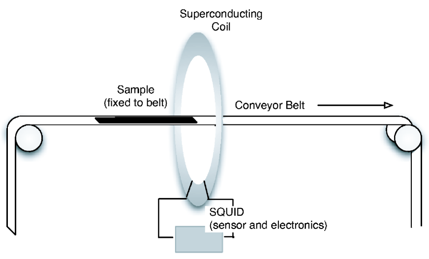
Figure 1: The schematic diagram shows the principle of the method. The conveyor belt travelled in steps of typically 5 cm until the sample traversed completely the superconducting coil. At each step the conveyor belt stopped for $1$ sec before the current in the superconducting coil (magnetometer current) was read to avoid the effects of eddy currents. The time for each step was typically $3$ secs.

For the direct search reported here we use the fact that heavily ionising magnetic monopoles produced in $e^{+}p$ collisions may stop in the beam pipe surrounding the H1 interaction point at HERA. The binding energy of monopoles which stop in the material of the pipe (aluminium in the years 1995-1997) is expected to be large [36] and so they should remain permanently trapped provided that they are stable. The beam pipe was cut into long thin strips which were each passed through a superconducting coil coupled to a Superconducting Quantum Mechanical Interference Device (SQUID). Fig. 1 shows a schematic diagram illustrating the principle of the method used. Trapped magnetic monopoles in a strip will cause a persistent current to be induced in the superconducting coil by the magnetic field of the monopole, after complete passage of the strip through the coil. In contrast, the induced currents from the magnetic fields of the ubiquitous permanent magnetic dipole moments in the material, which can be pictured as a series of equal and opposite magnetic charges, cancel so that the current due to dipoles returns to zero after passage of the strip.

The aluminium beam pipe used in 1995-1997 was exposed to a luminosity of $62\pm 1\mathrm{pb}^{-1}$. The beam pipe around the interaction point had a diameter of 9.0 cm and thickness 1.7 mm in the range $-0.3<z<0.5$ m and a diameter of 11.0 cm and thickness 2 mm in the range $0.5<z<2.0$ m. During HERA operations it was immersed in a 1.15 T solenoidal magnetic field which was directed parallel to the beam pipe, along the $+z$ direction. This length of the pipe, covering $-0.3<z<+2.0$ m, was cut into 45 longitudinal strips each of length on average of 573 mm ($\sim 2$ mm was lost at each cut). The central region ($-0.3<z<0.3$ m) was cut into 15 long strips of width $\sim 18$ mm, two of which were further divided into 32 short segments varying in length from 1 to 10 cm. The downstream region ($0.3<z<2.0$ m) was divided into 3 longitudinal sections each of which was cut into 10 long strips of width $\sim 32$ mm. The long strips and short segments were each passed along the axis of the 2G Enterprises type 760 magnetometer [37] at the Southampton Oceanography Centre, UK. This is a warm bore device with high sensitivity and low noise level. The samples of strips and segments were passed through the magnetometer in steps, pausing after each step, after which the current in the superconducting loop was measured. The residual persistent current after the complete traversal of a sample through the loop was measured by taking the difference in the measured current after and before passage. The readings for each sample were repeated several times. This allowed the reproducibility of the results to be studied so that random flux jumps and base line drifts could be identified. Any real monopole trapped in the pipe would give a consistent and reproducible current step.

A long, thin solenoid, wound with copper wire on a cylindrical copper former, was used to assess the sensitivity of the SQUID magnetometer to a monopole. The magnetic field outside of the ends of a long solenoid is similar to that produced by a monopole. A solenoid can thus be considered as possessing two oppositely charged “pseudopoles” of pole strength $g=N\cdot I\cdot S/g_{D}$ in units of the Dirac magnetic charge. Here $N$ is the number of turns per metre length, $I$ is the current and $S$ is the cross sectional area of the coil and $g_{D}=3.3\times 10^{-9}$ Ampère-metres is the Dirac magnetic charge introduced above. Hence the current and radius of the solenoid can be chosen to mimic the desired pole strength. To calibrate, the solenoid was stepped through the magnetometer. Data were taken with different currents subtracting the measurements with zero current to correct for the dipole impurities in the coil and its former. The measured increase in current in the magnetometer following the passage of one end of the solenoid was found to vary linearly with the pseudopole strength. Four coils, the details of which are given in table 1, were used at different times for the calibration procedure. Fig. 2 shows the magnetometer current divided by the solenoid pole strength as a function of the pole strength in units of $g_{D}$. There is a good consistency between the calibrations and the magnetometer is linear over more than 2 orders of magnitude in pole strength. The uncertainty on the point at the lowest pole strength is large because the current step size is small at such a low excitation of the calibration coil. Small differences, at the level of $\sim 0.03g_{D}$, of the current readings occurred between traversals, presumably due to the system picking up specks of slightly magnetised dust between the traversals. Such differences show up as noise for low excitations but are less important at higher excitation of the calibration coil. The mean values of the calibration factor, together with the root mean square deviations, from each coil are given in table 1.

To simulate trapped monopole behaviour the long solenoid was placed along a beam pipe strip and both were passed (jointly) through the magnetometer. Only one end of the calibration solenoid was allowed to traverse the magnetometer hence simulating the passage of a monopole in the strip. Fig. 3 shows the absolute value of the measured magnetometer current as the strip alone was stepped through and when pseudopoles of values $2.3g_{D}$ and $-2.3g_{D}$ were attached to the strip. The large structure at the centre comes from the magnetic fields from the permanent magnetic dipole moments in the aluminium. The final current persists when the pseudopoles are present. When the pseudopoles are absent the current returns to zero despite the very large permanent dipole moments. The inset of Fig. 3 shows the value of the measured current (on a linear scale) as the strip leaves the magnetometer coil. The values of current for these pseudopole strengths are equal and opposite and at the value expected from the calibration performed purely with the solenoid. This proves that a magnetic monopole attached to the beam pipe would have been detected by the magnetometer.

3 Results

3.1 Magnetometer Scans

The data were taken in four separate sets, taking just over one day for each set: in December 2002, January 2003, May 2003 and January 2004. In the first two sets of data (Dec. 2002 and Jan. 2003) all the strips from the central beam pipe, covering $-0.3<z<0.3$ m, were passed through the magnetometer once for each measurement. The values of the residual persistent current were computed from the difference between the first reading, typically $\sim 20$ cm before the strip entered the magnetometer, and the last reading which came typically $\sim 30$ cm after the strip left the magnetometer. These were then converted to Dirac Monopole units ($g_{D}$) by dividing by the calibration constant, determined as described above. The results for the long strips are shown in Fig. 4. In the first dataset (Dec. 2002) only single measurements were made on each long strip (except strip 13) and these are shown as open circles in Fig. 4. Two of the strips measured showed persistent currents of value expected from the passage of a magnetic charge of about $+0.7g_{D}$. Here a positive pole is defined to be a North seeking pole, i.e. one that is accelerated in the $+z$ direction by the H1 magnetic field. All the strips were then remeasured several times in the second set of data (Jan. 2003), shown as closed circles in Fig. 4. None of them (except a single reading for strip 3) showed a persistent current after traversal through the magnetometer. It was therefore assumed that the observed persistent currents during the first set had been caused by random jumps in the base line of the magnetometer electronics. It can be seen from Fig. 4 that none of the strips showed a persistent current which appeared consistently in more than one reading. Fig. 5 shows the results of the measurements on the 32 short segments from the central beam pipe. Sample 6 showed a reading at $\sim 0.5g_{D}$ for the first measurement but the measurement was compatible with zero when it was remeasured. It was therefore assumed that the first reading was due to a base line shift. We concluded that none of the long strips or short segments showed any consistent signal for a monopole in multiple readings and therefore that there were no magnetic monopoles trapped in the central section of the beam pipe.

In the third and fourth sets of data (May 2003, Jan. 2004) the strips from the downstream beam pipe were investigated. In these sets of data the magnetometer measurements proved to be less stable. This was probably due to the induced currents from the large permanent dipole moments encountered which caused the magnetometer to lose its memory of the zero level. The permanent dipole moments in the downstream beam pipe were found to be much larger than those in the central section. These dipole moments were all observed to be aligned along the H1 magnetic field, i.e. in the same direction as the proton beam. In these datasets the strips were passed through twice, first with the strip length parallel to the proton beam, termed $+z$ end first, and then with the strip aligned in the opposite direction, i.e. the length antiparallel to the proton beam direction, termed $-z$ end first. Fluctuations of the base level of size of $0.7g_{D}$ were observed to happen much more frequently than for the central beam pipe section (Dec. 2002 and Jan. 2003 data) and in a more systematic way. Fluctuations of $-0.7g_{D}$ were consistently present for the traversal with the $-z$ end first and fluctuations of $+0.7g_{D}$ were observed in the first $25\%$ of the traversals with the $+z$ end first but absent in the remaining $75\%$ of the readings in this orientation. To check that a monopole would have been seen, even in these adverse conditions, the long calibration coil was placed on a strip and the procedure repeated. The expected deviations from the calibration coil were seen superimposed on the base line shifts, confirming that a trapped monopole would have been seen had it existed, even in these conditions.

The permanent dipole moments in the downstream strips gave readings in the magnetometer up to 3 orders of magnitude larger than the final persistent current expected from a Dirac monopole. This is larger than those seen in Fig. 3. It was found that the base line shifts could be avoided by demagnetising the strips in a low frequency decreasing magnetic field of initial strength 0.1 T. This is less than $10\%$ of the H1 magnetic field. The binding energy of monopoles in aluminium, the main constituent of the beam pipe, is thought to be hundreds of keV [36] compared to those of atoms which are at the eV level. Hence it was thought that such magnetic fields would be unable to dislodge a trapped monopole. All the strips were therefore subject to such a demagnetising field and remeasured. Demagnetisation was found to reduce the permanent dipole moments in the aluminium strips by about a factor of 20. After this procedure no further base line shifts were observed after passage of a strip.

Fig. 6 shows all the readings of persistent current after demagnetisation plotted against sample number. The strips were passed through several at a time for these data. Sample 17 consists of the 13 strips of the central beam pipe (shown individually in Fig. 4) passed through the magnetometer as a bundle. It is concluded from Figs. 5 and 6, that no monopole of strength greater than 0.1 Dirac magnetic charge unit had stopped in any of the measured pieces which constituted $93\pm 3\%$ of the total beam pipe. The remainder was lost in the cutting procedure.

3.2 Upper Limits on the measured Cross Sections

To derive an upper limit on the measured cross section it is necessary to compute the acceptance, i.e. the fraction of the monopoles produced which would have been detected. A model of the production process is therefore needed. Two models were used to compute the acceptance by Monte Carlo technique. In each of these a monopole - antimonopole ($M\bar{M}$) pair was assumed to be produced by a photon-photon interaction. The first model (model A) assumed spin 0 monopole pair production by the elastic process $e^{+}p\rightarrow e^{+}M\bar{M}p$ through the interactions of a photon radiated from each of the electron and proton. The proton was assumed to have the simple dipole form factor $1/(1+Q^{2}/0.71\mathrm{GeV}^{2})$, where $Q^{2}$ is the negative square of the four momentum transferred to the proton. The second model (model B) assumed spin 1/2 monopole pair production by the inelastic process $e^{+}p\rightarrow e^{+}M\bar{M}X$ (where $X$ is any state) through a photon-photon fusion interaction with a photon radiated from the electron and one radiated from a quark in the proton. The photon is radiated with a simple distribution given by $(1-\eta)^{5}/\eta$, with $\eta$ the fraction of the proton’s energy carried by the photon. While the models implement the kinematic correlations in each event it should be noted that they depend on perturbation theory and therefore the predicted cross sections are unreliable, as mentioned previously. Events were generated according to model A using the programme CompHEP [38] and using a dedicated programme for model B. The generated final state particles were tracked through the H1 magnetic field to the beam pipe. If the thickness of beam pipe traversed was greater than the calculated range of the monopole in aluminium, it was assumed to stop. In this way the fraction of monopoles, which were detected by stopping in the beam pipe, was computed.

Monopoles experience a force $g{\bf B}$ in a magnetic field ${\bf B}$. With the field aligned along the $z$ axis they have a parabolic trajectory with

$$z(r)-z_{v}=0.5\frac{g|{\bf B}|r^{2}}{eP_{T}\beta_{T}}+\frac{r}{\tan\theta_{0}}$$ (1)

where $z_{v}$ is the $z$ coordinate of the vertex and $z(r)$ is the coordinate of a point on the trajectory at distance $r$ from the proton beam. The transverse momentum and tranverse velocity of the monopole are $P_{T}$ and $\beta_{T}$, respectively. The initial angle of the monopole to the proton beam direction is $\theta_{0}$ and $e$ is the unit of electric charge. In this equation $g$ is the magnetic pole strength which is negative (positive) for South (North) poles which decelerate (accelerate) in the $+z$ direction in the H1 magnetic field. The geometric acceptance is the fraction of the monopoles which traverse the beam pipe in the sampled length. The total acceptance is this fraction times the fraction which stop in the pipe. The range of monopoles in aluminium was computed by integrating the stopping power, $dE/dx$, given in [28] adjusted for the electron density in aluminium. Fig. 7 shows the computed range (normalised to mass), for monopoles of strength $g_{D}$, versus $P/M=\beta\gamma$ where $P$ and $M$ are the momentum and mass of the monopole, respectively, and $\beta,\gamma$ are its velocity factors. The stopping power was computed in [27, 28, 29] by classically considering the long range monopole interactions with atomic electrons and hence the result is unaffected by the limitations of the use of perturbation theory.

Figs. 8 and 9 show the total efficiency for stopping a monopole in the beampipe for models A and B, respectively. These were computed for magnetic charges of $1$, $2$, $3$ and $6g_{D}$, using the range calculations shown in Fig. 7, divided by the square of the monopole charge considered. The choice of magnetic charges was motivated by the Dirac quantisation condition [1] or the Schwinger modification [18] applied to the electron as the fundamental unit of electric charge (magnetic charges = $1g_{D}$ and $2g_{D}$) or to the $d$ quark as the fundamental unit of electric charge (magnetic charges = $3g_{D}$ and $6g_{D}$). The acceptance increases rapidly as the magnetic charge increases since larger charges have higher $dE/dx$ so that a greater fraction of the monopoles stop in the beam pipe. Hence the curve for $6g_{D}$ will also be approximately the acceptance for higher charged monopoles. The acceptance for South poles is somewhat larger than that for North poles since they decelerate in the H1 magnetic field, losing some energy, so that they stop more readily in the beam pipe. Higher mass monopole pairs are produced at smaller angles to the proton beam and tend to hit the downstream beam pipe. However, they are more energetic than for lower masses. Hence high masses with low magnetic charge pass through the downstream pipe whereas higher magnetic charges stop. This accounts for the rise in the acceptance at higher masses for magnetic charges of $2g_{D}$ and $3g_{D}$. The efficiencies for model A tend to be smaller than those for model B since in the latter the monopoles have a smaller mean transverse momentum than in the former which leads to a greater fraction of monopoles stopping in the beam pipe.

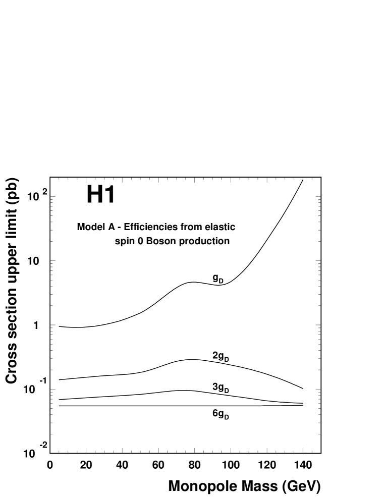
Figure 10: Upper limits on the cross section, determined within the context of model A, for monopole-antimonopole pair production in $e^{+}p$ collisions as a function of monopole mass for monopoles of strength $g_{D}$, $2g_{D}$, $3g_{D}$ and $6g_{D}$ or more.

The upper limit on the cross section for monopole-antimonopole pair production was derived within the context of each model, as follows. The failure to observe a monopole candidate means that there is an upper limit of 3 monopole pair events produced at the 95$\%$ confidence level. The cross section upper limit is then calculated from this, taking into account the uncertainties in the measured integrated luminosity, in the fraction of the pipe surviving the cutting procedure, and the statistical uncertainty in the acceptance computed from the models described above. Here the acceptance is the fraction of the monopole pairs which produce either one or both monopoles which stop in the beam pipe. Fig. 10 shows the upper limit on the cross section at 95$\%$ confidence level for monopoles of strength $1$, $2$, $3$ and $6g_{D}$ using acceptances determined from model A. Fig. 11 shows the upper limits determined using the acceptances from model B.

Several other experiments have also produced limits on monopole production cross sections for different masses and charges[9, 10, 12, 13, 14, 15, 16, 33]. However, owing to the lack of a reliable field theory for monopole production, different model assumptions were made in their derivations. Furthermore, although a universal production mechanism for monopole production can be postulated, comparisons of cross section limits in processes as diverse as $e^{+}p$, $p\bar{p}$ and $e^{+}e^{-}$ are difficult. This is the first search in $e^{+}p$ collisions. It could provide a sensitive testing ground for magnetic monopoles if a monopole condensate is responsible for quark confinement [6].

4 Conclusions

A direct search for magnetic monopoles produced in $e^{+}p$ collisions at HERA at a centre of mass energy of $\sqrt{s}=300$ GeV has been made for the first time. Monopoles trapped in the beam pipe surrounding the interaction point were sought using a SQUID magnetometer which was sensitive down to 0.1 Dirac magnetic charges ($0.1g_{D}$). No monopole signal was observed. Upper limits on the monopole pair production cross section have been set for monopoles with magnetic charges from $1$ to $6g_{D}$ or more and up to a mass of 140 GeV within the context of the models described.

5 Acknowledgement

We are grateful to the HERA machine group whose outstanding efforts have made this experiment possible. We thank the engineers and technicians for their work in constructing and now maintaining the H1 detector, our funding agencies for financial support, the DESY technical staff for continual assistance and the DESY directorate for support and for the hospitality which they extend to non-DESY members of the collaboration. We thank Andrew Robertson of the Southampton Oceanography Centre for making the SQUID magnetometer available to us and for his assistance and hospitality. We are indebted to Barbara Maher and Vassil Karloukovski of the University of Lancaster Geography Department and Gordon Donaldson and Colin Pegrum of the University of Strathclyde Physics Department for valuable discussions and assistance during the early part of the experiment.

Table 1: Description of the calibration coils.

Coil	1	2	3	4
Core diam.(mm)	6.08	3.15	2.1	2.1
Coil length (mm)	700	700	300	300
Wire diam.(mm) (including insulation)	0.18	0.18	0.1	0.1
Turns per metre	11000	11000	10000	30000
Coil area ($S$ mm2) (including wire)	32.6	9.7	3.80	4.54
Uncertainty in area	3.3$\%$	6.0$\%$	10$\%$	10$\%$
Mean magnetometer current per $g_{D}$	$1.10$	$1.09$	$1.11$	$1.11$
(arbitrary units)
R.M.S. deviation of the readings	0.016	0.024	0.030	0.017

Figure 2: The magnetometer current divided by the calibration pole strength as a function of the calibration pole strength for the four coils used (see table 1 for details of the coils).

Figure 3: The absolute (unsigned) value of the calibrated magnetometer current on a logarithmic scale versus step position ($z_{m}$) for a strip from the central beam pipe region ($-0.3<z<0.3\mbox{\rm~{}m}$). The solid line shows the measurements with the long strip alone. The closed (open) points show the measurements with the long strip together with the calibration solenoid excited to simulate a pole of strength $+2.3g_{D}$ ($-2.3g_{D}$). The inset shows the signed measurements of the calibrated magnetometer currents versus the step position for $z_{m}>0.8$ m on a linear scale. The expected persistent currents for monopoles of strength $\pm 2.3g_{D}$ are shown by the arrow on the logarithmic plot and by the numbers in the margin on the inset linear plot.

Figure 4: The measured persistent current (in units of $g_{D}$) in each strip, after passage through the magnetometer, plotted against strip number for 13 strips of the central beam pipe. Some of the strip numbers are offset for clarity. It can be seen that none of the fluctuations observed in single readings occured consistently in other readings on the same strip showing that no trapped monopole was present.

Figure 5: The measured persistent currents (in units of $g_{D}$), after passage through the magnetometer, plotted against sample number for the two strips of the central beam pipe which were cut into short segments. It can be seen that none of the fluctuations observed in single readings occured consistently in other readings on the same sample showing that no trapped monopole was present.

Figure 6: The measured persistent currents in the long strips in units of $g_{D}$, after passage through the magnetometer, against sample number after the samples had been demagnetised (see text). Samples 1-16 consisted of several long strips (usually two or three) from the downstream beam pipe bundled together. Sample 17 consisted of the thirteen long strips of the central beam pipe bundled together. These are shown individually in Fig. 4 before demagnetisation. All pieces of beam pipe tested are included in this plot except the short segments shown in Fig. 5. None of the readings indicate the presence of a magnetic monopole.

Figure 7: The ratio of the range to mass of a monopole of charge $g_{D}$ in aluminium versus $\beta\gamma$. The range was calculated from the stopping power, $dE/dx$, in Fig. 1 of [28], adjusted to the electron density in aluminium.

Figure 8: The efficiency for stopping monopoles of strength $g_{D}$, $2g_{D}$, $3g_{D}$ and $6g_{D}$ or more computed according to the monopole pair production model A.

Figure 9: The efficiency for stopping monopoles of strength $g_{D}$, $2g_{D}$, $3g_{D}$ and $6g_{D}$ or more computed according to the monopole pair production model B.

Figure 11: Upper limits on the cross section for monopole-antimonopole pair production in $e^{+}p$ collisions, determined within the context of model B, as a function of monopole mass for monopoles of strength $g_{D}$, $2g_{D}$, $3g_{D}$ and $6g_{D}$ or more.

References

-
[1]
P. A. M. Dirac,
Proc. Roy. Soc. Lond. A 133, 60 (1931) and
Phys. Rev. 74 (1948) 817.
Alternative derivations of the Dirac quantisation condition can be found
in
J.D. Jackson, Classical Electrodynamics, (John Wiley, New York, 1962); M. Kaku, Quantum Field Theory, a Modern Introduction (Oxford University Press, New York, 1993). -
[2]
R. D. Sorkin,
Phys. Rev. Lett. 51 (1983) 87;
D. J. Gross and M. J. Perry, Nucl. Phys. B 226 (1983) 29. - [3] E. Bergshoeff, E. Eyras and Y. Lozano, Phys. Lett. B 430 (1998) 77 [arXiv:hep-th/9802199].
-
[4]
G. ’t Hooft,
Nucl. Phys. B 79 (1974) 276;
A. M. Polyakov, JETP Lett. 20 (1974) 194 [Pisma Zh. Eksp. Teor. Fiz. 20 (1974) 430]. -
[5]
H. Minakata,
Phys. Lett. B 155 (1985) 352;
J. L. Lopez, Rept. Prog. Phys. 59 (1996) 819 [arXiv:hep-ph/9601208]. -
[6]
Y. Nambu,
Phys. Rev. D 10 (1974) 4262;
S. Mandelstam, Phys. Rept. 23 (1976) 245;
A. M. Polyakov, Nucl. Phys. B 120 (1977) 429;
G. ’t Hooft, Nucl. Phys. B 190 (1981) 455. - [7] K. Hagiwara et al. [Particle Data Group Collaboration], Phys. Rev. D 66 (2002) 010001.
- [8] H.V. Klapdor-Kleingrothaus and K. Zuber, Particle Astrophysics (The Institute of Physics, UK, 1999).
- [9] M. Bertani et al., Europhys. Lett. 12 (1990) 613.
- [10] G. R. Kalbfleisch, K. A. Milton, M. G. Strauss, L. P. Gamberg, E. H. Smith and W. Luo, Phys. Rev. Lett. 85 (2000) 5292 [arXiv:hep-ex/0005005].
- [11] B. Abbott et al. [D0 Collaboration], Phys. Rev. Lett. 81 (1998) 524 [arXiv:hep-ex/9803023].
- [12] P. Musset, M. Price and E. Lohrmann, Phys. Lett. B 128 (1983) 333.
- [13] W. Braunschweig et al. [TASSO Collaboration], Z. Phys. C 38 (1988) 543.
- [14] K. Kinoshita, M. Fujii, K. Nakajima, P. B. Price and S. Tasaka, Phys. Lett. B 228 (1989) 543.
- [15] K. Kinoshita et al., Phys. Rev. D 46 (1992) 881.
- [16] J. L. Pinfold, R. Du, K. Kinoshita, B. Lorazo, M. Regimbald and B. Price, Phys. Lett. B 316 (1993) 407.
- [17] M. Acciarri et al. [L3 Collaboration], Phys. Lett. B 345 (1995) 609.
- [18] J. S. Schwinger, Phys. Rev. 144 (1966) 1087, Phys. Rev. 173 (1968) 1536 and Science 165 (1969) 3895.
-
[19]
P. C. M. Yock,
Int. J. Theor. Phys. 2 (1969) 247;
A. De Rujula, R. C. Giles and R. L. Jaffe, Phys. Rev. D 17 (1978) 285;
D. Fryberger, Hadronic J. 4 (1981) 1844. - [20] T. G. Rizzo and G. Senjanovic, Phys. Rev. Lett. 46 (1981) 1315, Phys. Rev. D 24 (1981) 704 [Erratum-ibid. D 25 (1982) 1447], and Phys. Rev. D 25 (1982) 235.
- [21] J. Preskill, Ann. Rev. Nucl. Part. Sci. 34 (1984) 461.
- [22] E. J. Weinberg, D. London and J. L. Rosner, Nucl. Phys. B 236 (1984) 90.
- [23] T. W. Kirkman and C. K. Zachos, Phys. Rev. D 24 (1981) 999.
-
[24]
Y. S. Yang,
Proc. Roy. Soc. Lond. A 454 (1998) 155 and
Solitons in Field Theory and Nonlinear Analysis
(Springer Monographs in Mathematics, 2001);
Y. M. Cho, “Analytic electroweak dyon,” arXiv:hep-th/0210298. - [25] F. A. Bais and W. Troost, Nucl. Phys. B 178 (1981) 125.
- [26] T. Banks, M. Dine, H. Dykstra and W. Fischler, Phys. Lett. B 212 (1988) 45.
- [27] S. P. Ahlen, Phys. Rev. D 14 (1976) 2935.
- [28] S. P. Ahlen, Phys. Rev. D 17 (1978) 229.
- [29] S. P. Ahlen and K. Kinoshita, Phys. Rev. D 26 (1982) 2347.
-
[30]
See, for example
B. Cabrera,
Phys. Rev. Lett. 48 (1982) 1378;
A. D. Caplin, M. Hardiman, M. Koratzinos and J. C. Schouten, Nature 321 (1986) 402; V. A. Balkanov et al. [BAIKAL collaboration], Nucl. Phys. Proc. Suppl. 91 (2000) 438 [arXiv:astro-ph/0011313];
M. Ambrosio et al. [MACRO Collaboration], Eur. Phys. J. C 25 (2002) 511 [arXiv:hep-ex/0207020]. - [31] L.W. Alvarez et al., Science 167 (1970) 701.
- [32] P. H. Eberhard, R. R. Ross, L. W. Alvarez and R. D. Watt, Phys. Rev. D 4 (1971) 3260.
- [33] R. R. Ross, P. H. Eberhard, L. W. Alvarez and R. D. Watt, Phys. Rev. D 8 (1973) 698.
- [34] A. De Rujula, Nucl. Phys. B 435 (1995) 257 [arXiv:hep-th/9405191].
- [35] L. P. Gamberg, G. R. Kalbfleisch and K. A. Milton, “Difficulties with photonic searches for magnetic monopoles,” arXiv:hep-ph/9805365.
- [36] L. P. Gamberg, G. R. Kalbfleisch and K. A. Milton, Found. Phys. 30 (2000) 543 [arXiv:hep-ph/9906526].
- [37] URL:http://www.2genterprises.com.
- [38] A. Pukhov et al., “CompHEP: A package for evaluation of Feynman diagrams and integration over multi-particle phase space. User’s manual for version 33”, arXiv:hep-ph/9908288.