THE ANTINUCLEON–NUCLEON INTERACTION
AT LOW ENERGY: ANNIHILATION DYNAMICS

The general properties of antiproton–proton annihilation at rest are presented, with special focus on the two-meson final states. The data exhibit remarkable dynamical selection rules: some allowed annihilation modes are suppressed by one order of magnitude with respect to modes of comparable phase-space. Various phenomenological analyses are reviewed, based on microscopic quark dynamics or symmetry considerations. The role of initial- and final-state interaction is also examined.

1 Introduction

1.1 Annihilation in hadron physics

Annihilation is a fascinating process, one of the most interesting in low-energy hadron physics, in which matter undergoes a transition from its baryon structure to one consisting solely of mesons. In the early days of antiproton physics, antinucleon–nucleon ($\overline{\mathrm{N}}\mathrm{N}$) annihilation was considered by analogy with positronium annihilation in QED, and described as a short-range process mediated by baryon exchange. Nowadays the quark model offers a drastic alternative, where the so-called “annihilation” does not imply actual annihilation of all incoming quarks and antiquarks, but simply results from their rearrangement into quark–antiquark pairs. Were quark rearrangement to be the leading mechanism, $\overline{\mathrm{N}}\mathrm{N}$ annihilation would be better considered by analogy with rearrangement collisions in atomic or molecular physics. Intermediate scenarios are however conceivable, where some of the incoming quarks and antiquarks annihilate, and new quark–antiquark pairs are created.

This review is part of a project devoted to strong interaction physics with low-energy antiprotons, as measured at the LEAR facility of CERN. A first part [1] was devoted to $\overline{\mathrm{N}}\mathrm{N}$ scattering and to antiprotonic hydrogen and deuterium. The present review covers the general properties of annihilation, the results on two-meson final states and their phenomenological analysis. A third article will concentrate on meson spectroscopy, as studied from multimeson final states of annihilation.

1.2 Historical considerations

Detailed studies of antiproton–proton annihilation at rest were carried out in the 1960’s, and the results are still significant for studies of annihilation dynamics and meson spectroscopy. These experiments were performed at the Brookhaven National Laboratory (BNL) and at CERN in Geneva by stopping antiprotons in bubble chambers. Analysis methods and early results were reviewed in detail by Armenteros and French [2], but many important results were not included. Later reviews [3, 4, 5] focused primarily on new concepts and developments and did not aim at a comprehensive description of all experimental data. The physics results on $\bar{\mathrm{p}}$N annihilation obtained from bubble chambers filled with $\mathrm{H}_{2}$ or $\mathrm{D}_{2}$ are included in our report.

In the 70’s, $\overline{\mathrm{N}}\mathrm{N}$ physics was dominated by claims for narrow baryonium states, which were not confirmed by more systematic searches. The motivation for quasi-nuclear $\overline{\mathrm{N}}\mathrm{N}$ states and for multiquark states preferentially coupled to $\overline{\mathrm{N}}\mathrm{N}$  and the experimental results have been reviewed extensively in several articles [6, 7, 8, 9, 10].

Research on $\bar{\mathrm{p}}\mathrm{p}$ annihilation was resumed in 1983 when LEAR came into operation. The Asterix collaboration investigated annihilation from P-states of the $\bar{\mathrm{p}}\mathrm{p}$ atom formed in H₂ gas with a 2$\pi$ electronic detector. The focus of the research was dynamical selection rules which will be discussed in some detail in Sec. 7. A broad resonance, called AX(1565), possibly a quasi-nuclear state, was discovered. The search for narrow states produced in annihilation at rest continued both at LEAR and KEK, eventually yielding negative answers.

In more recent years, two $4\pi$ spectrometers, Crystal Barrel (PS197) and Obelix (PS201), took data on $\bar{\mathrm{p}}\mathrm{p}$ annihilation at LEAR. The Crystal-Barrel research activity was directed towards annihilation at rest and in flight. Obelix investigated antiproton and antineutron [11] interactions at rest and with very low momenta. Nuclear physics was also an important part of the Obelix program.

The experimental progress was accompanied by active groups of theoreticians trying to understand the basic mechanisms responsible for annihilation. From a theoretical point of view annihilation is a very complicated process which is likely driven by both the underlying quark dynamics and by conventional hadronic interactions. If for instance, the $\overline{\mathrm{N}}\mathrm{N}$ potential is attractive in one partial wave, and repulsive in another, one expects annihilation from the former to be enhanced, and annihilation from the latter to be suppressed. Similar remarks hold for final state interactions with, in addition, the possibility of interferences between, for instance, primary $\rho$ mesons formed by $\bar{q}q$ pairs and $\rho$ mesons built from $\pi\pi$ final-state interactions. An accurate description for all annihilation rates seems therefore to be unlikely. It is hoped, however, that the leading mechanisms of annihilation will be identified, in particular to explain the so-called dynamical selection rules, the observation that some annihilation modes are strongly suppressed in certain partial waves, while still being allowed by energy and quantum-number conservation.

1.3 Outline

This review begins, in Sec. 2, with a presentation of the beams and detector facilities used to measure annihilation properties. In Sec. 3, we briefly summarise the properties of the mesons seen in annihilation experiments. Kinematics and conservation laws are reviewed in Sec. 4. The main features of annihilation, as seen in various experiments, are presented in Sec. 5, while Sec. 6 is devoted to a thorough review of the rates into various two-meson final states. The dynamical selection rules are presented and discussed in Sec. 7. Section 8 contains a critical survey of various approaches to annihilation mechanisms, and an analysis of what is learned from the systematics of two-body branching ratios. Some conclusions are presented in Sec. 9.

1.4 A guide to the literature

The physics mediated by antiprotons has been presented at many Conferences, in particular the NAN conferences, the LEAR Workshops, and the LEAP conferences resulting from the merging of these two series, as well as at some Schools [12, 13, 14, 15, 16, 17, 18, 19, 20, 21, 22, 23, 24, 25, 26, 27, 28, 29, 30, 31, 32, 33, 34, 35, 36, 37, 38, 39, 40].

The early review by Armenteros and French [2] remains a reference for early annihilation data. Before the completion of LEAR measurements and the final analysis of the data, important review articles became available; some concerning general aspects of LEAR physics [3, 10], whilst others specialised more on the annihilation process [4, 5]. Antineutron physics, including antineutron annihilation, is reviewed in [11]. A review devoted to annihilation in flight appeared recently [41].

2 Beams and experiments

2.1 Early experiments at CERN and BNL

Following the discovery of the antiproton in 1955, $\bar{\mathrm{p}}$ beams were rapidly developed and a first survey of antiproton annihilation on protons or neutrons was possible, as early as in the 1960’s, by stopping antiprotons in hydrogen- and deuterium-filled bubble chambers. These experiments demonstrated that $\bar{\mathrm{p}}\mathrm{p}$ annihilation is a powerful tool to discover meson resonances, even though only limited statistics were achieved. Some of the early results are still important, and it seems appropriate to include a short discussion as to how the data were obtained.

Two main experiments were carried out at that time: the first one at Brookhaven by a group from Columbia University and the other at CERN by a CERN–Collège de France collaboration. The experimental conditions were closely similar and it is sufficient to discuss just one of them.

The CERN bubble chamber, built at Saclay, had an illuminated volume of 80 cm in length, and of 30 cm in height and depth. Antiprotons from a separated antiproton beam of momentum 700$\,{\mathrm{Me\hskip-1.0ptV}\hskip-2.0pt/\hskip-1.0ptc}$ were moderated in a Cu degrader and stopped in the target. The chamber was situated in a magnetic field of $2.1\,$T. Due to the momentum spread in the incident beam and multiple scattering in the degrader and target, the stopping distribution was rather wide. A cut on a minimum track length of 5 cm guaranteed a minimum momentum resolution; the average track length was 16 cm. The intensity of the antiproton beam was adjusted to allow for several (3 or 4) annihilation events for each bubble chamber expansion. Three stereoscopic pictures were taken of each expansion to enable a three-dimensional reconstruction of the tracks.

Scanning the films and reconstructing events was a major enterprise. The spatial coordinates of four points for each track were measured from the films, with a precision of 80$\,\mu$m. From the coordinates the charged–particle momenta were determined. We estimate the momentum resolution for 928$\,{\mathrm{Me\hskip-1.0ptV}\hskip-2.0pt/\hskip-1.0ptc}$ pions from the reaction $\bar{\mathrm{p}}\mathrm{p}\to\pi^{+}\pi^{-}$ to be 25$\,{\mathrm{Me\hskip-1.0ptV}\hskip-2.0pt/\hskip-1.0ptc}$.

A total of $1.6\times 10^{6}$ events were recorded at CERN, $7.5\times 10^{5}$ at BNL. These numbers exceeded the scanning capabilities available at that time, and only a fraction of the data was analysed: about 80,000 events at CERN and 45,000 events at BNL. From the momentum of the incoming antiprotons their range was estimated and compared to the true range; thus contamination due to in flight annihilation could be avoided, or at least reduced.

The Brookhaven results are documented in Refs. [42, 43, 44, 45, 46, 47, 48, 49, 50]. At CERN, more aspects of the annihilation process were investigated, leading to a larger number of publications. An incomplete list of publications in refereed journals includes [51, 52, 53, 54, 55, 56, 57, 58, 59, 60, 61, 62, 63, 64, 65, 2, 66, 67, 68, 69, 70, 71, 72, 73, 74, 75, 76] for H₂-filled and [77, 78, 79, 80, 81, 82, 83, 84] D₂-filled chambers. Further publications discussed the interpretation of these results.

In the 1970’s, a first set of counter experiments were performed at BNL to study $\gamma$-rays from antiproton annihilation. Antiprotons from a separated beam were stopped in a liquid H₂ or D₂ target. Photons were detected by their conversion in Cu(Pb) plates sandwiched between scintillation counters. In some experiments a NaI detector, surrounded by scintillation counters, was used to measure $\gamma$-rays with better resolution. Data from the Rome–Syracuse collaboration, taken with the D₂-filled BNL bubble chamber, were analysed in parallel. Results can be found in [85, 86, 87, 88, 89, 90, 91, 92, 93, 94, 95, 96, 97, 98, 99, 100, 101].

2.2 Experiments at KEK

This experiment was designed to search for narrow lines in the momentum distributions of $\pi^{0}$ and $\eta$ from $\bar{\mathrm{p}}\mathrm{p}$ annihilation. The initial aim was to find narrow multiquark or quasi-nuclear bound states [102, 103, 104, 105]. Later, frequencies for annihilation into two narrow mesons were determined with both $\mathrm{H}_{2}$ [106, 107] and $\mathrm{D}_{2}$ [108] targets.

Figure 1: Side and end view of the KEK detector.

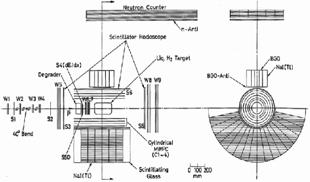
The layout of the experimental set-up is shown in Fig. 1. A full description of the detector can be found in [102, 103]. Antiprotons at 580$\,{\mathrm{Me\hskip-1.0ptV}\hskip-2.0pt/\hskip-1.0ptc}$, produced at the KEK 12 GeV proton synchrotron, were degraded in a graphite slab and stopped in a liquid $\mathrm{H}_{2}$ target of 14 cm diameter and 23 cm in length. The $\bar{\mathrm{p}}$ beam used double-stage mass separation and a contamination ratio of $\mathrm{e}\mu\pi/\bar{\mathrm{p}}\simeq 8$ was obtained with a typical stopping intensity of 270 $\bar{\mathrm{p}}$/synchrotron pulse. The charged particles produced in $\bar{\mathrm{p}}\mathrm{p}$ annihilation were detected with scintillation counter hodoscopes and tracked with cylindrical and planar multiwire proportional chambers whose total coverage was $93\%\times 4\pi$ sr. Photons were measured with a calorimeter consisting of 96 NaI(Tl) crystals surrounded by 48 scintillating glass modules and assembled into a half barrel [109], see Fig.1. The geometrical acceptance for $\pi^{0}$ increased from 10.5% at a $\pi^{0}$ energy of 500 MeV to 14.5% at 900 MeV. The overall energy resolution at FWHM for photons was approximately $\Delta E_{\gamma}/E_{\gamma}=6.2\%/(E_{\gamma}\mbox{ in \,GeV})^{1/4}$, for energies above 80 MeV.

Events were recorded when the detector signalled that a slow antiproton was incident on the liquid $\mathrm{H}_{2}$ target and one or two photons were measured in the NaI detector. A fast cluster counting logic counted the multiplicities of charged and neutral clusters separately, and if they satisfied preselected criteria the data was recorded. In some of the later experiments [107] an additional small $(1.3\%\times 4\pi$ sr.) BGO detector surrounded by NaI modules was used. No cluster counting logic was used in this case and the energy resolution (FWHM) was estimated to be $\Delta E_{\gamma}/E_{\gamma}=6.8\%/(E_{\gamma}\ \mbox{in \,GeV})^{1/4}$. As the NaI photon spectrometer has less than $2\pi$ acceptance, for measurements of two-body branching ratios it is not possible to detect both mesons. In this case the existence of the second meson and its mass are deduced from the inclusive energy spectrum recorded for a single $\pi^{0}$ or $\eta$.

2.3 Cooled antiproton beams

Early experiments with electronic detection techniques, including those carried out at KEK, used partially separated secondary antiproton beams produced from an external target. These beams were characterised by a relatively low rate of stopped antiprotons over a large volume and with a contamination of unwanted particles $\mathrm{e}\mu\pi/\bar{\mathrm{p}}\simeq 100$ in the earliest experiments to $\mathrm{e}\mu\pi/\bar{\mathrm{p}}\simeq 8$ in the more recent ones. This situation was transformed by the availability of cooled antiproton beams at CERN, together with the construction and operation of the LEAR facility.

A description of the cooled antiproton beams used at CERN has been given in a previous review article [1]. For a proton beam of 23$\,{\mathrm{Ge\hskip-1.0ptV}\hskip-2.0pt/\hskip-1.0ptc}$ incident on a Be target, antiprotons are produced with a broad maximum in momentum at 3.5$\,{\mathrm{Ge\hskip-1.0ptV}\hskip-2.0pt/\hskip-1.0ptc}$. The use of cooling allows these antiprotons to be decelerated to low momenta whilst keeping the same flux. Additionally, cooling gives the antiproton beams a small size and a reduced momentum.

The LEAR facility was constructed at CERN to handle pure antiproton beams in the momentum range from 105$\,{\mathrm{Me\hskip-1.0ptV}\hskip-2.0pt/\hskip-1.0ptc}$ to 2000$\,{\mathrm{Me\hskip-1.0ptV}\hskip-2.0pt/\hskip-1.0ptc}$ with small physical size and a typical momentum spread of $\Delta p/p\sim 0.1\%$. This small momentum spread for low momentum protons gave a very small stopping region in liquid $\mathrm{H}_{2}$ and $\mathrm{D}_{2}$ targets and also enabled gas targets to be used. The use of gas targets is particularly important since the fraction of P-state annihilation is considerably increased in gaseous $\mathrm{H}_{2}$ targets due to the reduced effect of Stark mixing. An ultra-slow extraction system enabled essentially DC beams to be produced, with spills typically lasting several hours. Typical beam intensities were in the range $10^{4}$ to $10^{6}$ $\bar{\mathrm{p}}$/sec. The beam purity was 100%.

The LEAR project was approved by CERN in 1980, and in July 1983 the first antiproton beams were delivered to users. After a break in 1987, to construct a new Antiproton Collector (ACOL) which resulted in a flux gain of a factor of 10, the facility was operated until the end of 1996, when it was closed for financial reasons. The Asterix, Obelix and Crystal Barrel (CBAR) experiments were all carried out at LEAR; Asterix in the first, Obelix and Crystal Barrel in the second phase.

2.4 Detectors at LEAR

2.4.1 PS 171: The Asterix experiment

Liquid targets were used in both the bubble chamber and counter experiments described earlier (Sec. 2.1 and 2.2). In liquid H₂ or D₂, annihilation occurs at rest and is preceded by capture of an antiproton by a hydrogen or deuterium atom. Collisions between the protonium atom and H₂ molecules induce transitions from high orbital angular momentum states via Stark mixing; and this mixing is fast enough to ensure dominant capture from S-wave orbitals. In H₂ gas, the collision frequency is reduced and P-wave annihilation makes significantly larger contributions. In particular at very low target pressures the P-wave fractional contribution is very large. Alternatively, rather pure samples of P-wave annihilation can also be studied by coincident detection of X-rays emitted in the atomic cascade of the $\bar{\mathrm{p}}\mathrm{p}$ system (which feed mostly the 2P level).

The Asterix experiment was designed to study $\bar{\mathrm{p}}\mathrm{p}$ annihilation from P-wave orbitals by stopping antiprotons in H₂ gas at room temperature and pressure and observing the coincident X-ray spectrum. The detector, shown in Fig. 2, consisted of the following main components:

1. A gas target of 45 cm length and 14 cm in diameter contained the full $\bar{\mathrm{p}}$ stop distribution for an antiproton beams at 105$\,{\mathrm{Me\hskip-1.0ptV}\hskip-2.0pt/\hskip-1.0ptc}$.

2. The target was surrounded by a X-ray drift chamber (also used to improve the tracking capability and for particle identification via dE/dx). The energy resolution of the detector for 8 keV X-rays was about 20%. Pions and kaons could be separated up to 400$\,{\mathrm{Me\hskip-1.0ptV}\hskip-2.0pt/\hskip-1.0ptc}$. The target and X-ray drift chamber were separated by a 6 $\mu$m aluminised mylar foil to guarantee gas tightness and good X-ray transmission even at low energies.

3. Charged particles were tracked in a set of seven multi-wire proportional chambers, partly with cathode readout to provide spatial resolution along the wires. The momentum resolution for $\bar{\mathrm{p}}\mathrm{p}\to\pi^{+}\pi^{-}$ events at 928$\,{\mathrm{Me\hskip-1.0ptV}\hskip-2.0pt/\hskip-1.0ptc}$ was 3%.

4. A one-radiation-length lead foil in front of the outer chambers permitted reconstruction of the impact points of photons.

5. Two end-cap detectors with three wire planes and cathode readout on both sides gave large solid-angle coverage. A lead foil was mounted behind the first chamber. The end cap detectors were used to identify $\gamma$’s but not for reconstruction of charged tracks.

6. The assembly was situated in a homogeneous magnetic field of 0.8 Tesla.

Figure 2: Side and front view of the PS172 Asterix detector.

With the experimental resolution of the detector, there was nearly no background for fully-constrained final states and up to 14% for final states with one missing $\pi^{0}$.

The main data sets taken with the Asterix detector consisted of $1.38\times 10^{6}$ events with two long tracks (passing at least the first five chambers) without triggering on X-rays, $2.13\times 10^{6}$ events with two long tracks with a trigger on X-rays, and $1.89\times 10^{6}$ events with four long tracks and with the X-ray trigger. The “long-track” criterion guaranteed that the particles reached the outermost chambers and gave optimum momentum resolution. The X-ray enhancing trigger had an efficiency of 25%; one quarter of the triggered events had — after all cuts — an identified low-energy X-ray. There was a contamination from Bremsstrahlung X-rays of about 15% in the X-ray data sample.

The detector is fully described in [110]. Physics results were published in [111, 112, 113, 114, 115, 116, 117, 118, 119, 120, 121, 122, 123, 124, 125, 126].

2.4.2 PS 201: The Obelix experiment

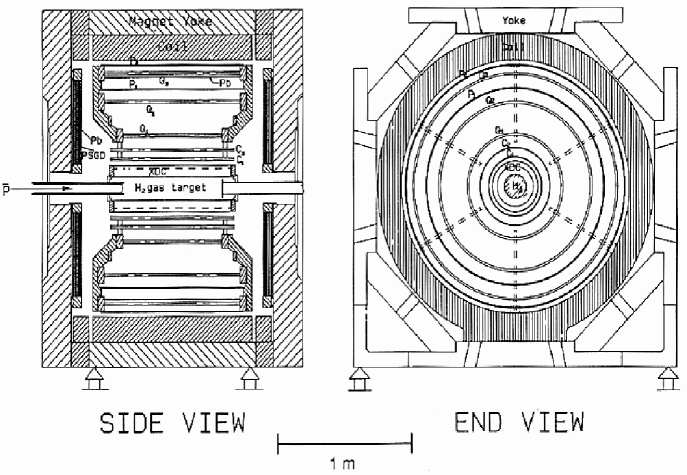
The layout of the Obelix spectrometer is shown in Fig. 3. A full description of the detector can be found in [127, 128]. It consists of four sub-detectors arranged inside and around the open-axial field magnet which had previously been used for experiments at the ISR. The magnet provides a field of 0.5 T in an open volume of about 3 m³. The subdetectors are:

1. A spiral projection chamber (SPC): an imaging vertex detector with three-dimensional readout for charged tracks and X-ray detection. This detector allowed data to be taken with a large fraction of P-wave annihilation, and to measure angular correlations between X-rays from the $\bar{\mathrm{p}}\mathrm{p}$ atomic cascade and annihilation products.

2. A time-of-flight (TOF) system: two coaxial barrels of plastic scintillators consisting of 30 (84) slabs positioned at a distance of 18 cm (136 cm) from the beam axis; a time resolution of 800 ps FWHM is achieved.

3. A jet drift chamber (JDC) for tracking and particle identification by dE/dx measurement with 3280 wires and flash-analog-to-digital readout. The chamber was split into two half-cylinders (160 cm in diameter, 140 cm long). The intrinsic spatial resolution was $\sigma_{z}=12\,$mm, $\sigma_{r\phi}=200\,\mu$m; the momentum resolution for monoenergetic pions (with 928$\,{\mathrm{Me\hskip-1.0ptV}\hskip-2.0pt/\hskip-1.0ptc}$) from the reaction $\bar{\mathrm{p}}\mathrm{p}\to\pi^{+}\pi^{-}$ was found to be 3.5%.

4. A high-angular-resolution gamma detector (HARGD) [127]. The calorimeter consisted of four modules made of layers of $3\times 4\,\mathrm{m}^{2}$ lead converter foils with planes of limited streamer tubes as the active elements. Twenty converter layers, each 3 mm thick, were used corresponding to a total depth of about $10$ radiation lengths. Due to their excellent spatial resolution, good energy resolution in the reconstruction of final states is obtained: $\pi^{0}$ are reconstructed with a mass resolution of $\sigma_{\pi^{0}}=10$ MeV and a momentum-dependent efficiency of 15 to 25%.

Figure 3: Schematic view of the Obelix experiment set-up. The numbers indicate the main components of the apparatus: the Open Axial Field magnet (1), the SPC (2, 4), the TOF (3), the JDC (5), the HARGD (6).

The detector system allowed a variety of targets to be used: a liquid H₂ target, a gaseous H₂ target at room temperature and pressure, also a target at low pressures (down to 30 mbar). The wide range of target densities could be used to study in detail the influence of the atomic cascade on the annihilation process. The H₂ could also be replaced by D₂. A further special feature of the detector was the possibility to study antineutron interactions. The $\bar{\mathrm{n}}$ beam was produced by charge exchange in a liquid H₂ target (positioned 2 m upstream of centre of the main detector). The intensity of the collimated beam was about $40\,\bar{\mathrm{n}}/10^{6}\bar{\mathrm{p}}$ of which about 30% interact in the central target. The $\bar{\mathrm{n}}$ beam intensity was monitored by a downstream $\bar{\mathrm{n}}$ detector.

The Obelix Collaboration had a broad program of experiments covering atomic, nuclear and particle physics [128]. The main results can be found in [11, 128, 129, 130, 131, 132, 133, 134, 135, 136, 137, 138, 139, 140, 141, 142, 143, 144, 145, 146, 147, 148, 149, 150, 151, 152, 153, 154, 155, 156, 157, 158, 159, 160, 161, 162].

2.4.3 PS 197: The Crystal Barrel experiment

The main objective of the Crystal Barrel experiment was the study of meson spectroscopy and in particular the search for glueballs (gg) and hybrid (g$\bar{q}q$) mesons produced in $\bar{\mathrm{p}}\mathrm{p}$ and $\bar{\mathrm{p}}\mathrm{d}$ annihilation at rest and in flight. Other objectives were the study of $\bar{\mathrm{p}}\mathrm{p}$ and $\bar{\mathrm{p}}\mathrm{d}$ annihilation dynamics and the study of radiative and rare meson decays. A particular feature of the experiment was its photon detection over a large solid angle with good energy resolution. Physics results are published in [4, 41, 163, 164, 165, 166, 167, 168, 169, 170, 171, 172, 173, 174, 175, 176, 177, 178, 179, 180, 181, 182, 183, 184, 185, 186, 187, 188, 189, 190, 191, 192, 193, 194, 195, 196, 197, 198, 199, 200, 201, 202, 203, 204, 205, 206, 207, 208, 209, 210, 211, 212, 213, 214, 215, 216, 217]

The layout of the Crystal Barrel spectrometer is shown in Fig. 4. A detailed description of the apparatus, as used for early data-taking (1989 onwards), is given in [218]. To study annihilation at rest, a beam of 200$\,{\mathrm{Me\hskip-1.0ptV}\hskip-2.0pt/\hskip-1.0ptc}$ antiprotons, extracted from LEAR, was stopped in a 4 cm long liquid hydrogen target at the centre of the detector. The whole detector was situated in a 1.5 T solenoidal magnet with the incident antiproton beam direction along its axis. The target was surrounded by a pair of multiwire proportional chambers (PWC’s) and a cylindrical jet drift chamber (JDC). The JDC had 30 sectors with each sector having 23 sense wires at radial distances between 63 mm and 239 mm. The position resolution in the plane transverse to the beam axis was $\sigma=125\,\mu$m. The coordinate along the wire was determined by charge division with a resolution of $\sigma=8$ mm. This gave a momentum resolution for pions of $\sigma/p\simeq 2\%$ at 200$\,{\mathrm{Me\hskip-1.0ptV}\hskip-2.0pt/\hskip-1.0ptc}$, rising to 7% at 1$\,{\mathrm{Ge\hskip-1.0ptV}\hskip-2.0pt/\hskip-1.0ptc}$ for those tracks that tracked all layers of the JDC. The JDC also provided $\pi$/K separation below 500$\,{\mathrm{Me\hskip-1.0ptV}\hskip-2.0pt/\hskip-1.0ptc}$ by ionisation sampling.

The JDC was surrounded by a barrel shaped calorimeter consisting of 1380 CsI(Tl) crystals in a pointing geometry. The CsI calorimeter covered the polar angles between $12^{\circ}$ and $168^{\circ}$ with full coverage in azimuth. The overall acceptance for shower detection was 0.95 $\times\ 4\pi$ sr. Typical photon energy resolutions for energy $E$ (in GeV) were $\sigma_{E}/E=2.5\%/E^{1/4}$, and $\sigma_{\phi,\theta}=1.2^{\circ}$ in both polar and azimuthal angles. The mass resolution was $\sigma\ =10$ MeV for $\pi^{0}$ and 17 MeV for $\eta\rightarrow 2\gamma$.

Figure 4: Overall layout of the Crystal Barrel detector showing (1) magnet yoke, (2) magnet coils, (3) CsI barrel, (4) jet drift chamber, (5) proportional chamber, (6) liquid hydrogen target, (7) one half of endplate. Left - longitudinal cross section; Right- transverse view.

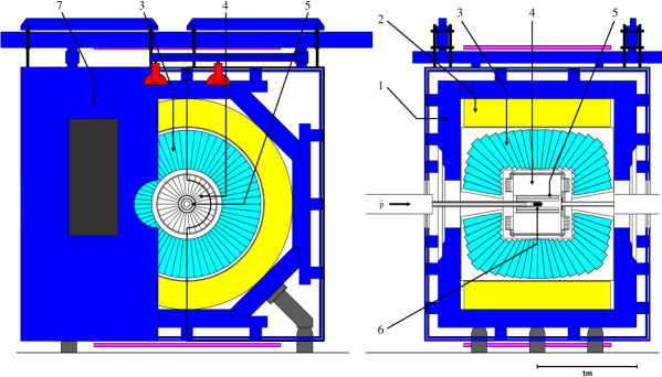
In 1995 the PWC’s were replaced by a microstrip vertex detector (SVTX) consisting of 15 single-sided silicon detectors, each having 128 strips with a pitch of $50\,\mu$m running parallel to the beam axis [219, 220]. (See [220, Fig. 1] for an overall view of the detector.) As well as giving improved identification of secondary vertices, this detector provided better vertex resolution in $r,\phi$ and improved momentum determination with a resolution $\Delta p/p$ for charged tracks of 3.4% at 0.8$\,{\mathrm{Ge\hskip-1.0ptV}\hskip-2.0pt/\hskip-1.0ptc}$ and 4.2% at 1.0$\,{\mathrm{Ge\hskip-1.0ptV}\hskip-2.0pt/\hskip-1.0ptc}$.

To study annihilation in hydrogen gas, the liquid target was replaced by a 12  cm long Mylar vessel with $230\mu$m thick walls and a $195\mu$m thick entrance window, containing hydrogen gas at room temperature and 12 bar pressure. A $55\mu$m thick Si detector was used to count the incident 105$\,{\mathrm{Me\hskip-1.0ptV}\hskip-2.0pt/\hskip-1.0ptc}$ antiproton beam.

A particular feature of the detector system was a multi-level trigger [218] on charged and neutral multiplicities and on invariant mass combinations of the neutral secondary particles. This allowed the suppression of well-known channels and the enhancement of rare channels of specific interest. The PWC/SVTX and the inner layers of the jet drift chamber determined the charged multiplicity of the final state. Events with long tracks could be selected to give optimum momentum resolution by counting the charged multiplicity in the outer layers of the JDC. A hardwired processor determined the cluster multiplicity in the CsI barrel, whilst a software trigger, which was an integral part of the calorimeter read out system, allowed a trigger on the total deposited energy in the barrel or on the $\pi^{0}$ or $\eta$ multiplicity.

Typical incident beam intensities were $\rm 10^{4}\,\bar{\mathrm{p}}/sec$ at 200$\,{\mathrm{Me\hskip-1.0ptV}\hskip-2.0pt/\hskip-1.0ptc}$ for stopping in liquid $\mathrm{H}_{2}$ or 105$\,{\mathrm{Me\hskip-1.0ptV}\hskip-2.0pt/\hskip-1.0ptc}$ when a 12 bar gas target was used. For experiments to study interactions in flight, larger intensities in the range from $10^{5}$ to $\rm 10^{6}\,\bar{\mathrm{p}}/sec$ were required at beam momenta in the range 600 to 1940$\,{\mathrm{Me\hskip-1.0ptV}\hskip-2.0pt/\hskip-1.0ptc}$.

A convenient summary of the data taken by the experiment, both at rest and in flight, for liquid $\mathrm{H}_{2}$  liquid $\mathrm{D}_{2}$ and gaseous $\mathrm{H}_{2}$ targets has been given by Amsler (see [4, Table 1]). Typical data sets contain $10^{6}$ to $2\times 10^{7}$ events.

2.5 Future experiments

With the closure of the LEAR facility in 1996, an era of intensive experimental study of low and medium energy antiproton annihilations came to an end. CERN has continued its involvement in the production of $\bar{\mathrm{p}}$ beams with the construction of the AD (Antiproton Decelerator) [221]. This provides $\bar{\mathrm{p}}$ beams with momentum from 100 to 300 $\,{\mathrm{Me\hskip-1.0ptV}\hskip-2.0pt/\hskip-1.0ptc}$ but without slow extraction. Slow extraction is not possible without making major modifications to the AD [222, 223]. The space for experiments [224] is very limited and the experimental program is solely devoted to the production of trapped antihydrogen and studies of the formation and cascade in light antiprotonic atoms.

For many years Fermilab has had the world’s most intense antiproton source. However the opportunities for medium energy $\bar{\mathrm{p}}$ physics have been very limited and experiments have focused on the observation and measurement of charmonium states. There has been no low-energy program. The possibility of building a new antiproton facility which could decelerate $\bar{\mathrm{p}}$ to below 2$\,{\mathrm{Ge\hskip-1.0ptV}\hskip-2.0pt/\hskip-1.0ptc}$ for injection into a new storage ring has been discussed [225]. The storage ring would be equipped with RF to decelerate $\bar{\mathrm{p}}$ down to the hundreds of $\,{\mathrm{Me\hskip-1.0ptV}\hskip-2.0pt/\hskip-1.0ptc}$ range. There are however, as yet, no firm plans to build such a facility.

The design of the Japan Proton Accelerator Research Complex (J-PARC, [226]) is well under way. The J-PARC project includes studies of particle and nuclear physics, materials science, life sciences and nuclear technology. The accelerator complex consists of an injection linac, a 3 GeV synchrotron and a 50 GeV synchrotron [227]. At this latter machine nuclear and particle physics experiments using neutrinos, antiprotons, kaons, hyperons and the primary proton beam are planned. At one stage it was hoped that the LEAR facility could be moved to J-PARC. However the LEAR ring is now required for the injection of heavy ions into the CERN LHC. It also seems likely that neutrino physics and the study of rare kaon decays will be topics for the first experiments at JFK and the construction of a dedicated low/medium energy antiproton facility is now some way off.

At the GSI laboratory in Darmstadt the construction of a new facility is planned and conditionally approved [228], the International Facility for Antiproton and Ion Research, FAIR. A conceptual design report [229] outlines a wide physics program and the envisaged accelerator complex. In particular a High Energy Storage Ring (HESR, [230]) will provide stored antiproton beams [231, 232, 233] in the range 3 to 15 $\,{\mathrm{Ge\hskip-1.0ptV}\hskip-2.0pt/\hskip-1.0ptc}$ with very good momentum resolution ($\Delta p/p\approx 10^{-5}$). The charm region is thus accessible with high rates and excellent resolution. A target inside the storage ring will be used, together with a large multi-purpose detector for neutral and charged particles with good particle identification [234]. Production and use of polarised antiprotons is a further future option for studying spin aspects of antiproton–proton scattering and annihilation. It is planned to broaden the program by including a low–energy component, FLAIR for the study of antimatter and highly-charged ions at low energies or nearly at rest.

3 Mesons and their quantum numbers

3.1 $q\bar{q}$ mesons and beyond

Since the annihilation process leads to production of mesons, it is useful to recall some basic definitions and properties of the meson spectrum.

Mesons are strongly-interacting particles with integer spin. The well established mesons have flavour structure and other quantum numbers which allows us to describe them as bound states of a quark and an antiquark. These valence quarks which describe the flavour content are surrounded by many gluons and quark–antiquark pairs. Other forms of mesons are also predicted to exist: glueballs should have no valence quarks at all; in hybrids, the hypothetical gluon string transmitting the colour forces between quark and antiquark is supposed to be dynamically excited; and multiquark states are predicted, described either as states of $(qq\bar{q}\bar{q})$ or higher valence-quark structure, or as meson–meson or baryon–antibaryon bound states or resonances. These unconventional states are presently searched for intensively; they are however not the subject of this review.

Quarks have spin $s=1/2$ and baryon number $B=1/3$, antiquarks $s=1/2$ and $B=-1/3$. Quark and antiquark combine to $B=0$ and to a spin triplet ($S=1$) or singlet ($S=0$). In conventional mesons, the total spin $\vec{S}$ of the quark $q$ and the antiquark $\bar{q}$, and the orbital angular momentum $\vec{L}$ between $q$ and $\bar{q}$ couple to the total angular momentum $\vec{J}$ of the meson: $\vec{J}=\vec{L}+\vec{S}$. Light mesons are restricted to $u,d$, and $s$ quarks.

3.2 Quantum numbers

Parity:

The parity $P$ of a meson involves the orbital angular momentum $L$ between quark and antiquark and the product of the intrinsic parities which is $P_{q}P_{\bar{q}}=-1$ for a fermion and its antiparticle:

$$P=(-1)^{L+1}.$$ (3.1)

Charge conjugation:

Neutral mesons are eigenstates of the charge conjugation operator

$$C=(-1)^{S+L}.$$ (3.2)

It turns out convenient to use the same sign convention within a multiplet. For instance, since $C\pi^{0}=\pi^{0}$, we choose $C\pi^{\pm}=\pi^{\mp}$, and $C\mathrm{K}^{0}=\overline{\mathrm{K}}{}{}^{0}$, while since $C\rho^{0}=-\rho^{0}$, we adopt $C\rho^{\pm}=-\rho^{\mp}$ and $C\mathrm{K}^{\star\,\pm}=-\overline{\mathrm{K}}{}{}^{\star\,\mp}$.

Isospin:

Proton and neutron form an isospin doublet and so do the up and the down quark. We define antiquarks by $\bar{u}\,=\,C\,u$ and $\bar{d}\,=\,C\,d$, antinucleons by $\rm\bar{p}\,=\,\it G\,\rm n$ and $\rm\bar{n}\,=\,\it G\,\rm p$. This means we use the ${\bf\bar{2}}$ representation of SU(2) for $\{\bar{u},\,\bar{d}\}$ and the ${\bf 2}$ representation for $\{\bar{\mathrm{p}},\,\bar{\mathrm{n}}\}$. See, e.g., [235] for a detailed discussion on phase conventions for isospin states of antiparticles. We obtain:

$$|\,I=1,I_{3}=1\,\rangle$$ =

=

=

= =

=

(3.3)

The $|\,\bar{{n}}{n}\,\rangle$ and $|\,\bar{{s}}{s}\,\rangle$ states have the same quantum numbers and mix to form two physical states. With $n$ we denote the two lightest quarks, $u$ and $d$, while $\rm n$ stands for the neutron.

The $G$-parity:

The $G$-parity is defined as charge conjugation followed by a rotation in isospin space about the $y$-axis,

$$G=Ce^{i\pi I_{y}}=(-1)^{I}C=(-1)^{L+S+I}~{},$$ (3.4)

and is approximately conserved in strong interactions. It is a useful concept since $G=(-1)^{n_{\pi}}$ for a system of $n_{\pi}$ pions. This generalises the selection rule for $\mathrm{e}^{+}\mathrm{e}^{-}\rightarrow n\gamma$ in QED, namely $C=(-1)^{n}$.

The ${\mathrm{a}}_{2}(1320)$, for instance, decays into $\rho\pi$ with $\rho\to\pi\pi$, hence into three pions, and into $\eta\pi$ with one pion in the final state. The ${\mathrm{a}}_{2}(1320)$ never decays into $\pi\pi$ or $\eta\pi\pi$: $G$-parity is conserved. The $\eta$ having $G=+1$ nevertheless decays into three pions; the $\omega$ has a small partial width for decays into two pions. These decay modes break isospin invariance; they vanish in the limit where $u$- and $d$-quark have equal masses and electromagnetic interactions are neglected. $\mathrm{K}\overline{\mathrm{K}}$ pairs may have $G=-1$ or $+1$.

3.3 Meson nonets

Mesons are characterised by their quantum numbers $J^{PC}$ and their flavour content. Quark-antiquark states with quantum numbers $J^{PC}$ are often referred to by the spectroscopic notation $n\,{}^{2S+1}L_{J}$ borrowed from atomic physics. In the light-quark domain, any $n\,{}^{2S+1}L_{J}$ leads to a nonet of states. Based on SU(3) symmetry, we expect an octet and a singlet. However, the $s$ quark is heavier than the $u$ and $d$ quark. This results into SU(3) breaking. The actual mesons can be decomposed either on a basis of SU(3) eigenstates or according to their $\bar{{u}}{u}$, $\bar{{d}}{d}$ and $\bar{{s}}{s}$ content.

3.3.1 The pseudoscalar mesons

The pseudoscalar mesons correspond to $J^{PC}=0^{-+}$ and $n\,{}^{2S+1}L_{J}$$=1^{1}S_{0}$. The nine orthogonal SU(3) eigenstates are shown in Fig. 5. The quark representation of the neutral members is

$$\pi^{0}=\frac{1}{\sqrt{2}}(\bar{{u}}{u}-\bar{{d}}{d})~{},\quad\eta_{8}=\sqrt{\frac{1}{6}}(\bar{{u}}{u}+\bar{{d}}{d}-2\bar{{s}}{s})~{},\quad\eta_{1}=\sqrt{\frac{1}{3}}(\bar{{u}}{u}+\bar{{d}}{d}+\bar{{s}}{s})~{}.$$ (3.5)

Figure 5: The nonet of pseudoscalar mesons.

The actual mesons $\eta$ and $\eta^{\prime}$ can be written as

 

$${{}|\,\eta\phantom{{}^{\prime}}\,\rangle=\cos\Theta_{\rm PS}|\,\eta_{8}\,\rangle-\sin\Theta_{\rm PS}|\,\eta_{1}\,\rangle}$$

  (3.6)

with the pseudoscalar mixing angle $\Theta_{\rm PS}$. A mixing angle $\Theta_{\rm PS}=\Theta_{\rm id}=\arctan(1/\sqrt{2})$, called the ideal mixing angle, would lead to a decoupling $\eta\propto|\,\bar{{s}}{s}\,\rangle$ and $\eta^{\prime}\propto|\,\bar{{n}}{n}\,\rangle$. The $\eta$ and $\eta^{\prime}$ wave functions can be decomposed into the $\bar{{n}}{n}$ and $\bar{{s}}{s}$ basis. With $\Theta=\Theta_{\rm PS}-\Theta_{\rm id}+\pi/2$,

 

$${{}|\,\eta\phantom{{}^{\prime}}\,\rangle=\cos\Theta\,|\,\bar{{n}}{n}\,\rangle-\sin\Theta\,|\,\bar{{s}}{s}\,\rangle=X_{\eta\phantom{{}^{\prime}}}\,|\,\bar{{n}}{n}\,\rangle+Y_{\eta\phantom{{}^{\prime}}}\,|\,\bar{{s}}{s}\,\rangle}$$

  (3.7)

The mixing angle can be determined experimentally from $\eta$ and $\eta^{\prime}$ production and decay rates. It is shown in [236] that the quark flavour basis $\bar{{n}}{n}$ and $\bar{{s}}{s}$ is better suited to describe the data than the octet–singlet basis. The latter can describe data only by the introduction of a second mixing angle.

The $\eta$ and $\eta^{\prime}$ could also mix with other states, in particular radial excitations or glueballs. The $\eta^{\prime}$ is nearly a flavour singlet state and can hence couple directly to the gluon field; this has led to speculations that the $\eta^{\prime}$ (and to a lesser extend also the $\eta$) may contain a large fraction of glue. This requires an extension of the mixing scheme (3.7) by introduction of a non-$q\bar{q}$ or inert component, with a third state of unknown mass which could, e.g., be dominantly a glueball.

$$|\,\eta\phantom{{}^{\prime}}\,\rangle= X_{\eta\phantom{{}^{\prime}}}\,|\,\bar{{n}}{n}\,\rangle\qquad+\qquad Y_{\eta\phantom{{}^{\prime}}}\,|\,\bar{{s}}{s}\,\rangle\qquad+\qquad Z_{\eta\phantom{{}^{\prime}}}\,|\,\rm glue\,\rangle$$

$$|\,\eta^{\prime}\,\rangle= X_{\eta^{\prime}}\,|\,\bar{{n}}{n}\,\rangle\qquad+\qquad Y_{\eta^{\prime}}\,|\,\bar{{s}}{s}\,\rangle\qquad+\qquad Z_{\eta^{\prime}}\,|\,\rm glue\,\rangle$$

$$\mathrm{light\ quark}\quad\ \qquad\mathrm{strange\ quark}\qquad\ \qquad\mathrm{inert}$$

At present there is no convincing evidence for a glueball content in the $\eta^{\prime}$ wave function, and we will assume ${Z_{\eta}}$ and ${Z_{\eta^{\prime}}}$ to vanish, i.e., $Z_{\eta}=Z_{\eta^{\prime}}\sim 0$.

3.3.2 Other meson nonets

A meson nonet consists of five isospin multiplets. The pseudoscalar nonet, for instance, contains the pion triplet, two kaon doublets, the $\eta^{\prime}$ and the $\eta$. Well known are also the nonet of vector mesons with quantum numbers $J^{PC}=1^{--}$ (three $\rho$, four K^∗, $\phi$ and $\omega$), and the nonet of tensor mesons with quantum number $2^{++}$ (${\mathrm{a}}_{2}(1320)$, K${}_{2}^{*}(1430)$, f${}_{2}(1525)$, ${\mathrm{f}}_{2}(1270)$). In a spectroscopic notation, these are the 1${}^{3}{{\mathrm{S}}}_{1}$ and 1${}^{3}{{\mathrm{P}}}_{2}$ states. Both nonets have a nearly ideal mixing angle $\Theta_{\rm id}=35.3^{\circ}$ for which one meson is a purely $\bar{{n}}{n}$ and the other one a purely $\bar{{s}}{s}$ state. These are the $\omega$ and $\phi(1020)$, and the ${\mathrm{f}}_{2}(1270)$ and f${}_{2}(1525)$ mesons, respectively. Note that the mass difference between the $s\bar{s}$ and the $n\bar{n}$ state is about 250 MeV. This mass difference is due to the larger constituent mass of strange quarks.

The mixing angles for these meson nonets (all except the pseudoscalar nonet) are defined as

 

$${{}|\,\omega\,\rangle=\cos\Theta_{V}\,|\,\bar{{n}}{n}\,\rangle-\sin\Theta_{V}\,|\,\bar{{s}}{s}\,\rangle}$$

  (3.9)

In Table 1 some meson nonets are collected. The assignment shown here is reproduced from the quark-model description of Amsler and Wohl in [237] and represents one possible scenario. In particular the scalar-meson nonet is hotly debated [238, 239] but there are also open questions in the axial-vector nonet [240, 241] and for the radial excitations of vector [242] and pseudoscalar [243] mesons.

Table 1: The light mesons. The two mesons K_1A and K_1B mix to form the observed resonances K${}_{1}(1280)$ and K${}_{1}(1400)$. The scalar mesons resist an unambiguous classification; the scenario reproduced here assumes that the $\mathrm{a}_{0}(980)$ and $\mathrm{f}_{0}(980)$ are $\mathrm{K}\overline{\mathrm{K}}{}$ molecules or generated dynamically but are not $\bar{q}q$ states, that the $\mathrm{f}_{0}(1370)$ is a $\bar{q}q$ state and not generated dynamically, and that the $\mathrm{f}_{0}(1500)$ is a glueball. The $\mathrm{f}_{1}(1510)$ is discarded in the listing below. There are considerable difficulties for the nonets of pseudoscalar and vector radial excitations.

$L$	$S$	$J$	$n$	$I=1$	$I=1/2$	$I=0$	$I=0$	$J^{PC}$	$n^{2s+1}L_{J}$
0	0	0	1	$\pi$	$\mathrm{K}$	$\eta$	$\eta^{\prime}$	$0^{-+}$	$1{}^{1}{{\mathrm{S}}}_{0}$
0	1	1	1	$\rho$	$\mathrm{K}^{*}$	$\phi$	$\omega$	$1^{--}$	$1{}^{3}{{\mathrm{S}}}_{1}$
1	0	1	1	b${}_{1}(1235)$	$\mathrm{K}_{1B}$	h${}_{1}(1380)$	h${}_{1}(1170)$	$1^{+-}$	$1{}^{1}{{\mathrm{P}}}_{1}$
1	1	0	1	a${}_{0}(1450)$	$\mathrm{K}_{0}^{*}(1430)$	f${}_{0}(1710)$	f${}_{0}(1370)$	$0^{++}$	$1{}^{3}{{\mathrm{P}}}_{0}$
1	1	1	1	a${}_{1}(1260)$	$\mathrm{K}_{1A}$	f${}_{1}(1420)$	f${}_{1}(1285)$	$1^{++}$	$1{}^{3}{{\mathrm{P}}}_{1}$
1	1	2	1	a${}_{2}(1320)$	$\mathrm{K}_{2}^{*}(1430)$	f${}_{2}(1525)$	f${}_{2}(1270)$	$2^{++}$	$1{}^{3}{{\mathrm{P}}}_{2}$
2	0	2	1	$\pi_{2}(1670)$	$\mathrm{K}_{2}(1770)$	$\eta_{2}(1870)$	$\eta_{2}(1645)$	$2^{-+}$	$\rm 1^{1}D_{2}$
2	1	1	1	$\rho(1700)$	$\mathrm{K}^{*}(1680)$	$\phi(????)$	$\omega(1650)$	$1^{--}$	$\rm 1^{3}D_{1}$
2	1	2	1	$\rho_{2}(????)$	$\mathrm{K}_{2}(1820)$	$\phi_{2}(????)$	$\omega_{2}(????)$	$2^{--}$	$\rm 1^{3}D_{2}$
2	1	3	1	$\rho_{3}(1690)$	$\mathrm{K}^{*}_{3}(1780)$	$\phi_{3}(1850)$	$\omega_{3}(1670)$	$3^{--}$	$\rm 1^{3}D_{3}$
0	0	0	2	$\pi$(1370)	$\mathrm{K}(1460)$	$\eta(1440)$	$\eta(1295)$	$0^{-+}$	$2{}^{1}{{\mathrm{S}}}_{0}$
0	1	1	2	$\rho$(1450)	$\mathrm{K}^{*}(1410)$	$\phi(1680)$	$\omega$(1420)	$1^{--}$	$2{}^{3}{{\mathrm{S}}}_{1}$

3.3.3 The Gell-Mann–Okubo mass formula

The Gell-Mann–Okubo mass formula relates the masses of a meson nonet and its mixing angle. It can be derived by ascribing to mesons a common mass $M_{0}$ plus the (constituent) masses of the quark and antiquark it is composed of. The relation is written as

$$\tan^{2}\Theta=\frac{3M_{\eta}+M_{\pi}-4M_{K}}{4M_{K}-3M_{\eta^{\prime}}-M_{\pi}}\,.$$ (3.10)

Often, the linear GMO mass formula is replaced by the quadratic GMO formula which is given as above but with $M^{2}$ values instead of masses $M$. Note that in the limit of chiral symmetry quark masses are proportional to the mass square of the meson masses. The quadratic GMO formula reads

$$\tan^{2}\Theta=\frac{3M^{2}_{\eta}+M_{\pi}^{2}-4M_{K}^{2}}{4M_{K}^{2}-3M^{2}_{\eta^{\prime}}-M_{\pi}^{2}}\,.$$ (3.11)

Table 2 gives the mixing angles derived from the linear and quadratic GMO formula.

Table 2: Mixing angles of meson nonets

Nonet members	$\Theta_{\rm linear}$	$\Theta_{\rm quad}$
$\pi,\mathrm{K},\eta^{\prime},\eta$	$-23^{\circ}$	$-10^{\circ}$
$\rho,\mathrm{K}^{*},\phi\ ,\omega$	$\phantom{-}36^{\circ}$	$\phantom{-}39^{\circ}$
${\mathrm{a}}_{2}(1320),\mathrm{K}^{*}_{2}(1430),{\mathrm{f}_{2}}(1525),{\mathrm{f}_{2}}(1270)$	$\phantom{-}26^{\circ}$	$\phantom{-}29^{\circ}$
$\rho_{3}(1690),\mathrm{K}^{*}_{3}(1780),\phi_{3}(1850),\omega_{3}(1670)$	$\phantom{-}29^{\circ}$	$\phantom{-}28^{\circ}$

3.3.4 The Zweig rule

The “quark line rule”, or Zweig rule, is also called the “OZI rule”, after Okubo, Zweig and Iizuka, or even the “A–Z rule” to account for all the various contributions to its study. See, e.g., Ref. [244], for a comprehensive list of references. This rule has played a crucial role in the development of the quark model.

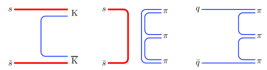
For instance, the $\phi(1020)$ is a vector meson with isospin $I=0$, seemingly similar to $\omega(780)$, but much narrower, in spite of the more favourable phase-space. It decays preferentially into $\mathrm{K}$$\overline{\mathrm{K}}$ pairs, and rarely into three pions. The explanation is that the $\phi(1020)$ has an almost pure $\bar{{s}}{s}$ content, and that the decay proceeds mostly with the strange quarks and antiquarks flowing from the initial state to one of the final mesons, as per Fig. 6, left, while the process with an internal $\bar{{s}}{s}$ annihilation (centre) is suppressed. The decay $\phi\to\pi\pi\pi$ is attributed to the main $\bar{{s}}{s}$ component being slightly mixed with a $\bar{q}q$ component, which in turn decays into pions by a perfectly allowed process (right).

The rule is quite strictly observed, as the non-strange width of the $\phi(1020)$ is less than 1 MeV! Even more remarkably, the rule works better and better for the charm and beauty analogues, for which the decay into naked-flavour mesons is energetically forbidden: the total width is only about 90 keV for the $\mathrm{J}/\Psi(c\bar{c})$ and 50 keV for $\Upsilon(b\bar{b})$.

Figure 6: Connected (left) and disconnected (centre) contribution to $\phi(1020)$ decay. The latter contribution to $\phi(1020)\to\pi\pi\pi$ can be described as an allowed decay from a small impurity in the wave function (right).

The magnitude of OZI violation in mesons is primarily described by the mixing angle, though an OZI violation from the decay amplitude cannot be excluded. The vector mesons, e.g., have a mixing angle of $\Theta_{V}=39^{\circ}$ which deviates from the ideal mixing angle $\Theta_{\rm id}$ by $\delta=3.7^{\circ}$. The physical $\phi(1020)$ is then written

$$|\,\phi\,\rangle=\cos\delta\,|\,\bar{{s}}{s}\,\rangle+\sin\delta\,|\,nnb\,\rangle.$$ (3.12)

If there are no $s$-quarks in the initial state we expect the production of $\phi$ mesons to be suppressed compared to $\omega$ production by $\sin^{2}\delta\simeq 0.042$. Indeed, a $\phi/\omega$ ratio of $0.0032\pm 0.0004$ was found at Argonne in the reaction $\pi^{-}\mathrm{p}\to\phi(\omega)\mathrm{p}$ at 6 GeV/ c [245]. This has to be compared with the extremely large values (up to 0.6 !) found in WA56 data on $\pi^{-}\mathrm{p}\to(\phi(\omega)+\pi)\mathrm{p}$ at 12 and 20 GeV/ c [246]. In $\bar{\mathrm{p}}\mathrm{p}$ annihilation at rest, the $\phi/\omega$ production ratios were found to depend strongly on the $\bar{\mathrm{p}}\mathrm{p}$ initial state and on the recoiling particles. These results will be discussed further in Sec. 8.

There is a wide consensus that ideal mixing and OZI rule can be, if not derived, at least justified from QCD, but there are different approaches: the $1/N_{c}$ expansion, where $N_{c}$ is the number of colour degrees of freedom, cancellations of loop diagrams, lattice simulations, instantons effects, etc. The generally accepted conclusion is that ideal mixing is nearly achieved for mesons, except in the scalar and in the pseudoscalar sectors. See, e.g., Ref. [247] and references there.

3.3.5 Meson decays

The decays of mesons belonging to a given nonet are related by SU(3) symmetry. The coefficients governing these relations are called SU(3) isoscalar factors and listed by the Particle Data Group [237]. We show here two simple examples.

A glueball is, by definition, a flavour singlet. It may decay into two octet mesons, schematically $1\rightarrow\ 8\times\ 8$. The isoscalar factors for this decay are

$$({\rm glueball})\rightarrow\ (\mathrm{K}\overline{\mathrm{K}}{}\ ,\ \pi\pi\ ,\ \eta_{8}\eta_{8}\ ,\ \overline{\mathrm{K}}{}\mathrm{K})=\frac{1}{\sqrt{8}}(2\ ,\ 3\ ,\ -1\ ,\ -2)^{1/2}\,.$$ (3.13)

Hence glueballs have squared couplings to $\mathrm{K}\overline{\mathrm{K}}{}$, $\pi\pi$ , $\eta_{8}\eta_{8}$ of 4 : 3 : 1 . The decay into two isosinglet mesons $\eta_{1}\eta_{1}$ has an independent coupling and is not restricted by these SU(3) relations. It could be large leading to the notion that the $\eta^{\prime}$ couples strongly to glueballs, and that $\eta^{\prime}$ are gluish. The decay into $\eta_{1}\eta_{8}$ is forbidden: a singlet cannot decay into a singlet and an octet meson. This selection rule holds for any pseudoscalar mixing angle: the two mesons $\eta$ and $\eta^{\prime}$ have orthogonal SU(3) flavour states and a flavour singlet cannot dissociate into two states which are orthogonal.

As a second example, we choose decays of vector mesons into two pseudoscalar mesons. We compare the two decays $\mathrm{K}^{*}\to\mathrm{K}\pi$ and $\rho\to\pi\pi$. These are decays of octet particles into two octet particles. This $8\rightarrow\ 8\times 8$ coupling is either symmetric ($8_{1}\to 8\times 8$) or antisymmetric ($8_{2}\to 8\times 8$) under the exchange of the final-state particles. The two pseudoscalars in $\mathrm{K}^{*}$ or $\rho$ decay having orbital momentum $\ell=1$, one should use the antisymmetric flavour coupling, $8_{2}\rightarrow\ 8\times 8$, whose isoscalar factors are

 

$${(\mathrm{K}^{*})\rightarrow\ (\mathrm{K}\pi\ \ \mathrm{K}\eta\ \ \pi\mathrm{K}\ \ \eta\mathrm{K})}$$

  (3.14)

Hence we derive $\mathrm{K}^{*}\to\mathrm{K}\pi+\pi\mathrm{K}$ $\propto 6$,   $\rho\to\pi\pi\ \propto\ 8$,   or

$$\frac{\Gamma_{\mathrm{K}^{*}\to\mathrm{K}\pi+\pi\mathrm{K}}}{\Gamma_{\rho\to\pi\pi}}=\frac{6}{8}\left(\frac{0.291}{0.358}\right)^{3}=0.40$$ (3.15)

The latter factor is the ratio of the decay momenta $q$ to the 3rd power. The transition probability is proportional to $q$; for low momenta (or point-like particles), the centrifugal barrier scales with $q^{2\ell}$ where $\ell$ is the orbital angular momentum.

From data we know that the width ratio is 0.34 and so the relations are fulfilled at the level of about $20\%$, a typical magnitude for SU(3) breaking effects. We have neglected many aspects: the transition rates are proportional to the squared matrix element (given by SU(3)) and the wave function overlap. The latter can be different for the two decays. Mesons are not point-like; the angular barrier factor should hence include Blatt–Weisskopf corrections [248]. An application of SU(3) to vector and tensor mesons can be found in [249].

4 Kinematics and conservation laws

In this section, we discuss the kinematics of annihilation into two, three, or more mesons, and the selection rules due to exactly or approximately conserved quantum numbers.

4.1 Kinematics

We consider annihilation at rest. The formalism below can be used for annihilation in flight in the centre of mass, if $2m$ is replaced by $s^{1/2}$, where $m$ is the proton or antiproton mass, and $s$ the usual Mandelstam variable $s=(\tilde{p}_{1}+\tilde{p}_{2})^{2}$ built of the four-momenta of the initial proton and antiproton.

If $m_{1}$, $m_{2}$, etc. denote the mass of the final mesons, annihilation is possible if

$$2m\geq m_{1}+m_{2}+\cdots~{},$$ (4.1)

Up to 13 pions could be produced.

4.1.1 Two-body annihilation

Figure 7: Kinematics for two-body annihilation

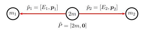
The notation is defined in Fig. 7. From the energy–momentum balance rewritten as $\tilde{p}_{2}=\tilde{P}-\tilde{p}_{1}$ and squared, one gets

 

$${{}E_{1}={4m^{2}-m_{2}^{2}+m_{1}^{2}\over 4m}~{},}$$

  (4.2)

In case of two identical mesons the momentum can be written in the form

$$|\vec{p}_{1}|=\sqrt{m^{2}-m_{1}^{2}}~{}.$$ (4.3)

The occurrence of two narrow mesons is easily observed due to the narrow momentum distribution of the two produced particles. Other annihilation modes such as $\rm p\bar{p}\to$ $\rho\pi$ or ${\mathrm{a}}_{2}(1320)$$\pi$ involve short-lived resonances. In these cases, the measurement of the annihilation frequency is more complicated.

Due to its relatively large mass, the antiproton-proton system possesses a large variety of two-body annihilation modes. In Table 3 we list the momenta of typical reactions. For broad resonances the momenta are calculated for the nominal meson masses. Some annihilation modes like $\bar{\mathrm{p}}\mathrm{p}\to\omega{\mathrm{f}}_{2}(1270)$ are at the edge of the phase space and only the part of the ${\mathrm{f}}_{2}(1270)$ below 1094 MeV is produced. They may, nevertheless, make a significant contribution to the annihilation process.

The mean decay length, $D_{l}=\gamma\beta c\tau=\hbar p/(m\Gamma)$, varies over a wide range. For $\rm p\bar{p}\to\pi^{0}\eta$, the mean path of the $\pi^{0}$ is $D_{l}=1\,$nm within the $\eta$ lifetime. Assume the $\eta$ then decays into $\pi^{+}\pi^{-}\pi^{0}$. Because of the large $D_{l}$ there will be no interaction between the $\pi^{0}$ recoiling against the $\eta$ and the pions from $\eta$-decays. In case of $\pi\rho$ annihilations, the recoil pion travels 7.5 fm within the $\rho$ mean live time, and rescattering of the primarily produced pion and pions from $\rho$ decays is unlikely. The situation is different for production of two short-lived high-mass mesons. In annihilation into $\mathrm{K}^{*}\overline{\mathrm{K}}{}^{*}+\mathrm{c.c.}$, the $\mathrm{K}^{*}$’s have moved only a mean distance of 1.3 fm when they decay and interactions between the kaons and pions from $\mathrm{K}^{*}$ decays are likely to occur.

Table 3: Momenta for $\bar{\mathrm{p}}\mathrm{p}$  annihilation at rest into two mesons.

Channel		Momentum	Channel		Momentum
$\bar{\mathrm{p}}\mathrm{p}\to$	$\pi^{0}\pi^{0}$	928.5 $\,{\mathrm{Me\hskip-1.0ptV}\hskip-2.0pt/\hskip-1.0ptc}$	$\bar{\mathrm{p}}\mathrm{p}\to$	$\rho\rho$	536.3 $\,{\mathrm{Me\hskip-1.0ptV}\hskip-2.0pt/\hskip-1.0ptc}$
	$\pi^{+}\pi^{-}$	927.8 $\,{\mathrm{Me\hskip-1.0ptV}\hskip-2.0pt/\hskip-1.0ptc}$		$\omega\rho$	527.5 $\,{\mathrm{Me\hskip-1.0ptV}\hskip-2.0pt/\hskip-1.0ptc}$
	$\pi^{0}\eta$	852.3 $\,{\mathrm{Me\hskip-1.0ptV}\hskip-2.0pt/\hskip-1.0ptc}$		$\omega\omega$	518.5$\,{\mathrm{Me\hskip-1.0ptV}\hskip-2.0pt/\hskip-1.0ptc}$
	$\mathrm{K}^{+}$$\mathrm{K}^{-}$	797.9 $\,{\mathrm{Me\hskip-1.0ptV}\hskip-2.0pt/\hskip-1.0ptc}$		$\eta\phi$	499.7 $\,{\mathrm{Me\hskip-1.0ptV}\hskip-2.0pt/\hskip-1.0ptc}$
	$\mathrm{K}^{0}\overline{\mathrm{K}}{}^{0}$	795.4 $\,{\mathrm{Me\hskip-1.0ptV}\hskip-2.0pt/\hskip-1.0ptc}$		$\pi$${\mathrm{f}}_{2}(1270)$	491.2 $\,{\mathrm{Me\hskip-1.0ptV}\hskip-2.0pt/\hskip-1.0ptc}$
	$\pi\rho$	773.2 $\,{\mathrm{Me\hskip-1.0ptV}\hskip-2.0pt/\hskip-1.0ptc}$		$\pi$${\mathrm{a}}_{2}(1320)$	459.9 $\,{\mathrm{Me\hskip-1.0ptV}\hskip-2.0pt/\hskip-1.0ptc}$
	$\pi^{0}\omega$	768.4 $\,{\mathrm{Me\hskip-1.0ptV}\hskip-2.0pt/\hskip-1.0ptc}$		$\eta^{\prime}\rho$	364.4 $\,{\mathrm{Me\hskip-1.0ptV}\hskip-2.0pt/\hskip-1.0ptc}$
	$\eta\eta$	761.0 $\,{\mathrm{Me\hskip-1.0ptV}\hskip-2.0pt/\hskip-1.0ptc}$		$\eta^{\prime}\omega$	350.5 $\,{\mathrm{Me\hskip-1.0ptV}\hskip-2.0pt/\hskip-1.0ptc}$
	$\eta\rho$	663.5 $\,{\mathrm{Me\hskip-1.0ptV}\hskip-2.0pt/\hskip-1.0ptc}$		$\rm\mathrm{K}^{*}\overline{\mathrm{K}}{}^{*}$	285.2 $\,{\mathrm{Me\hskip-1.0ptV}\hskip-2.0pt/\hskip-1.0ptc}$
	$\pi^{0}\eta^{\prime}$	658.7 $\,{\mathrm{Me\hskip-1.0ptV}\hskip-2.0pt/\hskip-1.0ptc}$		$\rho\phi$	280.3 $\,{\mathrm{Me\hskip-1.0ptV}\hskip-2.0pt/\hskip-1.0ptc}$
	$\eta\omega$	656.4 $\,{\mathrm{Me\hskip-1.0ptV}\hskip-2.0pt/\hskip-1.0ptc}$		$\omega\phi$	260.8 $\,{\mathrm{Me\hskip-1.0ptV}\hskip-2.0pt/\hskip-1.0ptc}$
	$\pi^{0}\phi$	652.4 $\,{\mathrm{Me\hskip-1.0ptV}\hskip-2.0pt/\hskip-1.0ptc}$		$\eta$${\mathrm{f}}_{2}(1270)$	206.2 $\,{\mathrm{Me\hskip-1.0ptV}\hskip-2.0pt/\hskip-1.0ptc}$
	$\rm\mathrm{K}\overline{\mathrm{K}}{}^{*}$	616.2 $\,{\mathrm{Me\hskip-1.0ptV}\hskip-2.0pt/\hskip-1.0ptc}$		$\eta$${\mathrm{a}}_{2}(1320)$	91.2 $\,{\mathrm{Me\hskip-1.0ptV}\hskip-2.0pt/\hskip-1.0ptc}$
	$\eta\eta^{\prime}$	546.1 $\,{\mathrm{Me\hskip-1.0ptV}\hskip-2.0pt/\hskip-1.0ptc}$		$\omega$${\mathrm{f}}_{2}(1270)$	See text

4.1.2 Three-body annihilation

Unlike the two-body case, the energy of a given particle can vary over a certain range. Even for equal masses, the symmetric star of Fig. 8 (left) is only a very particular case.

Figure 8: Notation for the kinematics of three-body annihilation (right). Even for equal masses, the symmetric star (left) is just one possibility among many others.

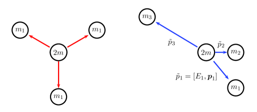
The minimal energy of particle 1, for instance, is obviously obtained when it is produced at rest and particles 2 and 3 share the remaining energy $2m-m_{1}$, as per Eq. (4.2), mutatis mutandis. However, the maximal value of $E_{1}$ does not correspond to either particle 2 or 3 being being produced at rest. Equation (4.2), if rewritten as

$$2mE_{1}=4m^{2}-m_{23}^{2}+m_{1}^{2}~{},$$ (4.4)

where $m_{23}$ is the invariant mass of the $\{2,3\}$ subsystem, indicates that $E_{1}$ is maximal, with value

$$\max E_{1}={4m^{2}-(m_{2}+m_{3})^{2}+m_{1}^{2}\over 4m}~{},$$ (4.5)

when $m_{23}$ is minimal, i.e., $m_{23}=m_{2}+m_{3}$, when particles 2 and 3 are at rest relative to each other.

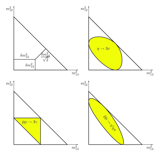
4.1.3 Dalitz plot

Energy conservation, rewritten for the kinetic part $T_{i}=E_{i}-m_{i}$ implies that

$$T_{1}+T_{2}+T_{3}=T=2m-m_{1}-m_{2}-m_{3}~{},$$ (4.6)

remains constant from one event to another. This property is fulfilled if $T_{i}$ is represented by the distance of a point to the $i^{\mathrm{th}}$ side of an equilateral triangle of height $T$, as in Fig. 9. We just saw that while $T_{1}=0$ is possible, $T_{1}=T$ contradicts momentum conservation, which requires

$$|p_{2}-p_{3}|\leq p_{1}\leq p_{2}+p_{3}~{}.$$ (4.7)

Saturating this inequality, i.e., fixing the three momenta $\vec{p}_{i}$ to be parallel, gives the boundary of the Dalitz plot, which corresponds to all possible sets $\{T_{i}\}$ allowed by energy and momentum conservation. In the non-relativistic limit, the frontier is a circle for identical particles, and an ellipsis for unequal masses, as shown in Fig. 9.

Figure 9: Definition of the Dalitz plot for kinetic energies (upper left), and boundary in the non-relativistic limit, for a decay into three identical particles (upper right) and for particles with masses in ratio [4:1:1] (lower left) or [7:4:1] (lower right), corresponding to the mass ratios for $\eta\to 3\pi$, $\eta^{\prime}\to\eta\pi\pi$ and $\bar{\mathrm{p}}\mathrm{p}\to\eta^{\prime}\eta\pi$, respectively.

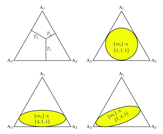
In the relativistic case, the shape of the Dalitz plot becomes more angular. For the (rare) $\bar{\mathrm{p}}\mathrm{p}\to 3\gamma$ decays, it reduces to a triangle limiting the middles of the sides. Using Eq. (4.4), the Dalitz plot can be rescaled to substitute the kinetic energies $T_{k}$ with the invariant masses $m_{ij}^{2}$, which fulfil

$$\sum_{i<j}m_{ij}^{2}=4m^{2}+m_{1}^{2}+m_{2}^{2}+m_{3}^{3}~{},\quad(m_{1}+m_{2})^{2}\leq m_{12}^{2}\leq(2m-m_{3})^{2}~{}.$$ (4.8)

Also, the equilateral frame is replaced in recent literature by rectangular triangles. Some examples are shown in Fig. 10.

Figure 10: Dalitz plots with relativistic kinematics: interpretation of the distances ($\delta m_{ij}^{2}$ represents the excess of $m_{ij}^{2}$ with respect to the minimal value $(m_{i}+m_{j})^{2}$), decays $\eta\to 3\pi$, $\bar{\mathrm{p}}\mathrm{p}\to 3\gamma$, and $\bar{\mathrm{p}}\mathrm{p}\to\eta^{\prime}\eta\pi$.

4.1.4 Multiparticle final state

The results on the energy range are easily generalised to more than three mesons in the final state. If $2m\geq m_{1}+m_{2}+\cdots+m_{n}$, annihilation into the $n$ mesons $\{m_{i}\}$ is allowed, and the energy of particle 1, for instance, is bounded by

$$m_{1}\leq E_{1}\leq{4m^{2}-(m_{2}+m_{3}+\cdots+m_{n})^{2}+m_{1}^{2}\over 4m}~{}.$$ (4.9)

4.2 Phase space

Heavier particles are less easily produced than lighter ones. Removing this obvious kinematical effect leads to a more meaningful comparison among various reaction rates. We give below some basic results. For a more detailed treatment, see, e.g., the reviews [237, 250].

The typical decay rate of protonium, of mass $2m$, into a set of $n$ mesons $\{m_{i}\}$ is given by

$$\Gamma={(2\pi)^{4-3n}\over 2^{2+n}m}\int|\mathcal{M}|^{2}\prod_{i=1}^{n}\mathrm{d}^{3}{p_{i}\over E_{i}}\,\delta^{4}(\tilde{P}-\tilde{p}_{1}-\cdots\tilde{p}_{n})~{}.$$ (4.10)

If $|\mathcal{M}|^{2}$ is removed, one obtains the phase-space integral. For two-body decays ($n=2$), $|\mathcal{M}|^{2}$ contains the non-trivial dynamical variations when going from one channel to another. For $n\geq 3$, $|\mathcal{M}|^{2}$ also contains information on the correlation or anticorrelation of momenta, allowing tests of scenarios for the formation of resonances, etc.

For $n=2$, the phase-space integral is evaluated in the c.o.m. frame [237] as

$$\Gamma={|\vec{p}_{1}|\over 32\pi m^{2}}\,|\mathcal{M}|^{2}~{}.$$ (4.11)

For $n=3$, the phase-space integral is conveniently expressed as an integral over two kinetic energies or, equivalently, two invariant 2-body masses, i.e., the variables used to draw the Dalitz plot. The result is [237]

$$\mathrm{d}\Gamma={|\mathcal{M}|^{2}\over(2\pi)^{3}16m}\mathrm{d}T_{1}\mathrm{d}T_{2}={|\mathcal{M}|^{2}\over(2\pi)^{3}256m^{3}}\mathrm{d}m_{12}^{2}\mathrm{d}m_{23}^{2}~{},$$ (4.12)

where an average over initial spins is implied. Unfortunately, measurements of annihilation at rest with a polarised protonium state have not been performed.

Equation (4.12) implies that for the fictitious dynamics where $|{\cal M}|$ is constant, the Dalitz plot in coordinates $\{T_{1},T_{2}\}$ or $\{m_{12}^{2},m_{23}^{2}\}$ is uniformly populated. Peaks in the population density indicate the formation of resonances, or at least constructive interferences of several dynamical contributions to the amplitude.

4.3 Conservation laws

Strong interactions obey very strictly conservation laws due to basic symmetries: energy $E$, momentum $\vec{p}$, angular momentum $J$, parity $P$ and charge conjugation $C$ are conserved, as well as flavours. Isospin is also a rather good symmetry. $G$-parity (or isotopic parity) is a combination of charge conjugation and isospin, $G=C\exp(-i\pi I_{2})$.

4.3.1 Partial waves

The algebra of $\overline{\mathrm{N}}\mathrm{N}$ quantum numbers is very similar to that of $\bar{q}q$ reviewed in the section on mesons. The partial wave ${}^{2I+1,2S+1}L_{J}$, where $L$ is the orbital momentum and $S$ the total spin has $C=(-1)^{L+S}$ (if the system is neutral), $P=(-1)^{L+1}$, and $G=(-1)^{L+S+I}$. This is summarised in Table 4, for S and P waves.

Table 4: Quantum numbers of the S and P partial waves (PW) of the $\overline{\mathrm{N}}\mathrm{N}$ system. The notation is ${}^{2I+1,2S+1}L_{J}$.

PW	${}^{1,1}{{\mathrm{S}}}_{0}$	${}^{3,1}{{\mathrm{S}}}_{0}$	${}^{1,3}{{\mathrm{S}}}_{1}$	${}^{3,3}{{\mathrm{S}}}_{1}$	${}^{1,1}{{\mathrm{P}}}_{1}$	${}^{3,1}{{\mathrm{P}}}_{1}$	${}^{1,3}{{\mathrm{P}}}_{0}$	${}^{3,3}{{\mathrm{P}}}_{0}$	${}^{1,3}{{\mathrm{P}}}_{1}$	${}^{3,3}{{\mathrm{P}}}_{1}$	${}^{1,3}{{\mathrm{P}}}_{2}$	${}^{3,3}{{\mathrm{P}}}_{2}$
$J^{PC}$	$0^{-+}$	$0^{-+}$	$1^{--}$	$1^{--}$	$1^{+-}$	$1^{+-}$	$0^{++}$	$0^{++}$	$1^{++}$	$1^{++}$	$2^{++}$	$2^{++}$
$I^{G}$	$0^{+}$	$1^{-}$	$0^{-}$	$1^{+}$	$0^{-}$	$1^{+}$	$0^{+}$	$1^{-}$	$0^{+}$	$1^{-}$	$0^{+}$	$1^{-}$

4.3.2 Simple rules

The simplest and most effective selection rule comes from $G$-parity. Only half of the partial waves, for instance, are candidates for annihilation into five pions, those with $G=-1$. Once $G$-parity is obeyed, one can generally match any set of quantum numbers by cleverly arranging the spins and internal orbital momenta of the mesons. Important exceptions are observed in channels involving a small number of spinless mesons or identical particles. We review these selection rules below. The reasoning was elaborated in the 60’s (see, for instance, [251, 252]) to identify the quantum numbers of meson resonances from their observed decays into a few mesons. The large angular acceptance and improved resolution of modern detectors forces us to consider higher multiplicities.

4.3.3 Two spinless mesons

For $\overline{\mathrm{N}}\mathrm{N}$$\rightarrow$ two scalars or two pseudoscalars, only natural parity $P=(-1)^{J}$ is allowed. For $\pi^{0}\pi^{0}$, $J$ has to be even; $I+J$ is even for $\pi^{-}\pi^{+}$, while there is no correlation between $I$ and $J$ for $\mathrm{K}^{-}\mathrm{K}^{+}$. For $\overline{\mathrm{N}}\mathrm{N}\rightarrow\mathrm{K}^{0}\overline{\mathrm{K}}{}{}^{0}$, one detects $\mathrm{K_{s}}$ or $\mathrm{K_{l}}$ and $C\!P$ invariance provides selection rules for $\mathrm{K_{s}}$$\mathrm{K_{s}}$ or $\mathrm{K_{s}}$$\mathrm{K_{l}}$ channels. The results are summarised in Table 5. Similarly, for $\overline{\mathrm{N}}\mathrm{N}\rightarrow$ scalar + pseudoscalar, only states with unnatural parity $P=(-1)^{J+1}$ contribute.

4.3.4 Identical vector mesons

For two identical vector mesons, the Pauli principle does not lead to further restrictions, once $G$ or $C$ conservation is enforced. Total spin $S=0$ or 2 of mesons implies even $\ell$ and opens the $J^{P}=0^{+},1^{+},2^{+},\ldots$ channels, while spin $S=1$ requires an antisymmetric space configuration and thus $J^{P}=0^{-},1^{-},2^{-},\ldots$ Note, however, that ${}^{1,3}{{\mathrm{P}}}_{1}\rightarrow\omega\omega$ (or $\phi\phi$, or $\rho^{0}\rho^{0}$) involves a total spin $S=2$ and an angular momentum $\ell=2$ in the final state.

Table 5: Allowed decays from S and P-wave protonium states into selected two-meson final states (FS).

FS

${}^{1,1}{{\mathrm{S}}}_{0}$

${}^{3,1}{{\mathrm{S}}}_{0}$

${}^{1,3}{{\mathrm{S}}}_{1}$

${}^{3,3}{{\mathrm{S}}}_{1}$

${}^{1,1}{{\mathrm{P}}}_{1}$

${}^{3,1}{{\mathrm{P}}}_{1}$

${}^{1,3}{{\mathrm{P}}}_{0}$

${}^{3,3}{{\mathrm{P}}}_{0}$

${}^{1,3}{{\mathrm{P}}}_{1}$

${}^{3,3}{{\mathrm{P}}}_{1}$

${}^{1,3}{{\mathrm{P}}}_{2}$

${}^{3,3}{{\mathrm{P}}}_{2}$

$\pi^{0}\pi^{0}$

$\surd$

$\surd$

$\pi^{-}\pi^{+}$

$\surd$

$\surd$

$\surd$

$\pi^{0}\eta^{(\prime)}$

$\surd$

$\surd$

$\eta^{(\prime)}\eta^{(\prime)}$

$\surd$

$\surd$

$\mathrm{K}^{-}\mathrm{K}^{+}$

$\surd$

$\surd$

$\surd$

$\surd$

$\surd$

$\surd$

$\mathrm{K_{s}}\mathrm{K_{l}}$

$\surd$

$\surd$

$\mathrm{K_{s}}\mathrm{K_{s}}$

$\surd$

$\surd$

$\surd$

$\surd$

$\pi^{0}\omega(\phi)$

$\surd$

$\surd$

$\eta^{(\prime)}\omega(\phi)$

$\surd$

$\surd$

$\pi^{0}\rho^{0}$

$\surd$

$\surd$

$\eta^{(\prime)}\rho^{0}$

$\surd$

$\surd$

$\pi^{\pm}\rho^{\mp}$

$\surd$

$\surd$

$\surd$

$\surd$

$\surd$

4.3.5 Symmetric multi-$\pi^{0}$ states

More delicate is the case of three or more $\pi^{0}$. This is no longer an academic problem, since these channels are seen in modern detectors. For instance, ${}^{1,1}{{\mathrm{S}}}_{0}$ has adequate $C$ and $G$ for decaying into $4\pi^{0}$. One can thus say that ${}^{1,1}{{\mathrm{S}}}_{0}\rightarrow 4\pi^{0}$ is not forbidden by charge conjugation. To claim that it is actually allowed, one should exhibit at least one example of a four-body wave function that is together symmetric and pseudoscalar. At first sight, this seems impossible. In fact, one can build such a wave function, with the desired coupling $\vec{\ell}_{1}+\vec{\ell}_{2}+\vec{\ell}_{3}=0$ of the internal orbital momenta, but with $\ell_{1}$, $\ell_{2}$ and $\ell_{3}$ not vanishing, as it will be explained shortly. As a first step, let us consider the $\pi^{0}+\pi^{0}+\pi^{0}$ case.

The method adopted below is simple, but a little empirical. We refer to Ref. [253] for a group-theoretical treatment. We tentatively write down minimal polynomials in the Jacobi variables with the required quantum numbers. Their angular-momentum content is then the lowest term in a systematic partial-wave expansion.

4.3.6 Three $\pi^{0}$

There is a copious literature on 3-body wave functions and their permutation properties. For instance, in the simple quark model of baryons, one should write down spatial wave functions with well-identified permutation symmetry, to be associated with spin, isospin and colour wave functions, to form a state with overall antisymmetry. Let $p$ be the parity of the orbital wave-function. In the harmonic-oscillator scheme [254], the symmetric states are labelled as $[56,J^{p}]$, and the allowed values of $J^{p}$ in the lowest multiplets with $N\leq 3$ quanta of excitation are $0^{+}$, $1^{-}$, $2^{+},\ldots$ [254]. There is no pseudoscalar $(J^{p}=0^{-}$), since to get $J=0$, the two internal orbital momenta $\ell_{1}$ and $\ell_{2}$ should be equal, and thus $p=(-1)^{\ell_{1}+\ell_{2}}=+1$. The states $J^{p}=1^{+}$ and $2^{-}$ are allowed [251, 252], but with complicated wave functions, since the coupling of internal momenta, $\vec{\ell}_{+}\\ vec{\ell}_{2}=\vec{J}$ is achieved with $\ell_{1}+\ell_{2}=8$ and $5$, respectively.

To show that $J^{p}=0^{+},\,1^{-}$ and $2^{-}$ are allowed for three bosons, it is sufficient to give explicit examples. The Jacobi variables

$$\vec{\rho}={\vec{p}}_{2}-{\vec{p}}_{1}~{},\quad\vec{\lambda}=(2{\vec{p}}_{3}-{\vec{p}}_{1}-{\vec{p}}_{2})/\sqrt{3}~{},$$ (4.13)

are built out of the individual momenta ${\vec{p}}_{i}$. $1\leftrightarrow 2$ exchange and circular permutation results in

$$(\vec{\lambda},\vec{\rho}\,)\rightarrow(\vec{\lambda},-\vec{\rho}\,),\ (-\vec{\lambda}\pm\sqrt{3}\vec{\rho},\,\mp\sqrt{3}\vec{\lambda}-\vec{\rho}\,)/2~{}.$$ (4.14)

A constant, or $\rho^{2}+\lambda^{2}$, is scalar and symmetric, leading to the existence of $J^{p}=0^{+}$ spatial wave functions. The vector $(J^{p}=1^{-})$

$$(\lambda^{2}-\rho^{2})\vec{\lambda}-(2\vec{\lambda}\!\cdot\!\vec{\rho}\,)\vec{\rho},$$ (4.15)

is also symmetric. The vector and axial vector

$$\vec{V}=(\lambda^{2}-\rho^{2})\vec{\rho}+(2\vec{\lambda}\!\cdot\!\vec{\rho}\,)\vec{\lambda},\quad\vec{W}=\vec{\rho}\times\vec{\lambda}~{},$$ (4.16)

are both antisymmetric and thus

$$V_{+}W_{+}$$ (4.17)

has $J=2$, $J_{z}=2$, and orbital parity $p=-1$, and is symmetric. In Eq. (4.17), we use the standard notation $V_{+}=-(V_{x}+iV_{y})/\sqrt{2}$.

For three pions, the parity is $P=-p$, once the intrinsic parities are taken into account. Hence $J^{P}=0^{-}$, $1^{+}$ and $2^{-}$ are allowed, i.e., ${}^{3,1}{{\mathrm{S}}}_{0}$, ${}^{3,3}{{\mathrm{P}}}_{1}$ and ${}^{3,3}{{\mathrm{P}}}_{2}$ can decay into $3\pi^{0}$.

4.3.7 $\overline{\mathrm{N}}\mathrm{N}\rightarrow 4\pi^{0}$

One first eliminates all channels but those with $C=G=+1$ and thus is restricted to $I=0$. While it seems $J^{P}=0^{+}$ or $2^{+}$ are obviously allowed, it seems at first rather difficult to enforce all requirements of permutation symmetry for $0^{-}$ and $1^{+}$. For instance, with the system of Jacobi coordinates consisting of $\vec{x}\propto{\vec{p}}_{2}-{\vec{p}}_{1}$, $\vec{y}\propto{\vec{p}}_{4}-{\vec{p}}_{3}$ and $\vec{z}\propto{\vec{p}}_{4}+{\vec{p}}_{3}-{\vec{p}}_{2}-{\vec{p}}_{1}$, $1\leftrightarrow 2$ and $3\leftrightarrow 4$ symmetries are simply translated into an even behaviour in $\vec{x}$ and $\vec{y}$, but the effect of transpositions like $1\leftrightarrow 3$ is not easily written down. The task is simplified by using the variables

$$\vec{u} = ({\vec{p}}_{4}+{\vec{p}}_{1}-{\vec{p}}_{2}-{\vec{p}}_{3})~{},$$

$$\vec{v} = ({\vec{p}}_{4}+{\vec{p}}_{2}-{\vec{p}}_{3}-{\vec{p}}_{1})~{},$$ (4.18)

$$\vec{w} = ({\vec{p}}_{4}+{\vec{p}}_{3}-{\vec{p}}_{1}-{\vec{p}}_{2})~{},$$

since the wave function simply has to survive the changes $\vec{u}\leftrightarrow\vec{v}$, $\vec{u}\leftrightarrow-\vec{v}$, $\vec{v}\leftrightarrow\vec{w}$, etc. The following wave functions can be written down

$$J^{P}=0^{-} (u^{2}-v^{2})(v^{2}-w^{2})(w^{2}-u^{2})\vec{u}\cdot(\vec{v}\times\vec{w})~{},$$

$$J^{P}=0^{+} 1~{},$$

$$J^{P}=1^{+} (u^{2}-v^{2})(v^{2}-w^{2})(w^{2}-u^{2})(\vec{u}\times\vec{v}+\vec{v}\times\vec{w}+\vec{w}\times\vec{u})~{},$$

$${\rm or}$$

$$(u^{2}-v^{2})(\vec{w}\times\vec{u})\times(\vec{w}\times\vec{v})+(v^{2}-w^{2})(\vec{u}\times\vec{v})\times(\vec{u}\times\vec{w})~{}$$

$$\phantom{(u^{2}-v^{2})(\vec{w}\times\vec{u})\times(\vec{w}\times\vec{u})}{}+(w^{2}-u^{2})(\vec{v}\times\vec{w})\times(\vec{v}\times\vec{u})~{}$$

$$J^{P}=2^{+} u_{+}^{2}+v_{+}^{2}+w_{+}^{2}~{}.$$

In summary ${}^{1,1}{{\mathrm{S}}}_{0}$, ${}^{1,3}{{\mathrm{P}}}_{0}$, ${}^{1,3}{{\mathrm{P}}}_{1}$, and ${}^{1,3}{{\mathrm{P}}}_{2}$ can decay into four neutral pions. One can probably establish these results in a more physical way, by symmetrising amplitudes written as a product of terms describing the successive steps of sequential decays, provided there is no cancellation when the overall Bose–Einstein symmetry is implemented. For instance, ${}^{1,1}{{\mathrm{S}}}_{0}\to\pi^{0}\mathrm{a}_{2}$ is allowed, with a relative angular momentum $\ell=2$. Also $\mathrm{a}_{2}\to\mathrm{f}_{2}\pi^{0}$, with $\ell^{\prime}=1$, and in turn, $\mathrm{f}_{2}\to\pi^{0}\pi^{0}$.

4.3.8 Five or more $\pi^{0}$

For $\bar{\mathrm{p}}\mathrm{p}\rightarrow 5\pi^{0}$, ${}^{3,1}{{\mathrm{S}}}_{0}$ and the triplet states ${}^{3,3}{{\mathrm{P}}}_{0,1,2}$ are allowed. We refer here to the paper by Henley and Jacobsohn [251]. Symmetric states are found in any $J^{p}$, sometimes with many internal excitations. In particular, it is difficult to produce five $\pi^{0}$ from $J^{p}=0^{-}$, corresponding to ${}^{3,3}{{\mathrm{P}}}_{0}$.

The pattern is seemingly generalisable for any number $n>5$ of identical pions. No state is strictly forbidden to decay into $n\,\pi^{0}$, but the transition is sometimes suppressed by the requirement of having many internal excitations in the final wave function.

4.4 Isospin considerations

We summarise here some results on isospin symmetry and its violation in $\bar{\mathrm{p}}\mathrm{p}$ annihilation.

4.4.1 Relations for two-body annihilation

Simple relations can be written down for two-body decays. Consider, for instance, two-pion events with a trigger on a X-ray, ensuring that annihilation takes place from a P-state of protonium. Isospin symmetry presumably holds for such pions since their energy is large compared to the $\pi^{\pm}-\pi^{0}$ mass differences, and Coulomb effects are likely to be negligible in the final state. Then $\pi\pi$ states from a $J^{P}=0^{+}$ or $2^{+}$ state are pure $I=0$, and

$$\mathrm{AF}_{\rm P}(\bar{\mathrm{p}}\mathrm{p}\to\pi^{+}\pi^{-})=2\,\mathrm{AF}_{\rm P}(\bar{\mathrm{p}}\mathrm{p}\to\pi^{0}\pi^{0})~{},$$ (4.20)

where the subscript P indicates annihilation from P-states only.

4.4.2 Relations for three-body annihilation

For more than two particles in the final state, there are usually more than one isospin amplitude contributing to the transition. Consider for instance

$$\bar{\mathrm{n}}\mathrm{p}\to\mathrm{K}^{+}\overline{\mathrm{K}}{}^{0}\pi^{0}~{},\ \ \mathrm{K}^{+}\mathrm{K}^{-}\pi^{+}~{},\ \ \mathrm{K}^{0}\overline{\mathrm{K}}{}^{0}\pi^{+}~{},$$ (4.21)

for which one can identify two amplitudes, one with $(\mathrm{K}\overline{\mathrm{K}}{})$ in a $I=0$ state, i.e.,

$$\mathcal{A}_{0}=\mathcal{A}(\bar{\mathrm{n}}\mathrm{p}\to(\mathrm{K}\overline{\mathrm{K}}{})^{0}\pi^{+})~{},\quad(\mathrm{K}\overline{\mathrm{K}}{})^{0}={\mathrm{K}^{+}\mathrm{K}^{-}-\mathrm{K}^{0}\overline{\mathrm{K}}{}^{0}\over\sqrt{2}}~{},$$ (4.22)

and another one where $(\mathrm{K}\overline{\mathrm{K}}{})$ has $I=1$

$$\mathcal{A}_{1}=\mathcal{A}\left[\bar{\mathrm{n}}\mathrm{p}\to{1\over\sqrt{2}}\mathrm{K}^{+}\overline{\mathrm{K}}{}^{0}\pi^{0}-{1\over 2}(\mathrm{K}^{+}\mathrm{K}^{-}\pi^{+}+\mathrm{K}^{0}\overline{\mathrm{K}}{}^{0}\pi^{+})\right]~{}.$$ (4.23)

One can extract the contribution of $\mathcal{A}_{0}$ and $\mathcal{A}_{1}$ to each of the final states and, after squaring, deduce (up to a common phase- space factor) that

 

$${\mathrm{AF}(\mathrm{K}^{+}\mathrm{K}^{-}\pi^{+})+\mathrm{AF}(\mathrm{K}^{0}\overline{\mathrm{K}}{}^{0}\pi^{+})}$$

  (4.24)

Hence

$$\mathrm{AF}(\mathrm{K}^{+}\mathrm{K}^{-}\pi^{+})+\mathrm{AF}(\mathrm{K}^{0}\overline{\mathrm{K}}{}^{0}\pi^{+})\geq\mathrm{AF}(\mathrm{K}^{+}\overline{\mathrm{K}}{}^{0}\pi^{0})~{},$$ (4.25)

the difference being the $I=0$ contribution. In other words, one gets often inequalities instead of equalities.

4.4.3 Isospin equalities for three-body final states

However, one may sometimes get equalities, either by straightforward Clebsch–Gordan recoupling or by more sophisticated methods. An example is antinucleon annihilation into two pions on deuterium. Lipkin and Peskin [255] have shown that

$$\sigma(\bar{\mathrm{p}}\mathrm{d}\to\pi^{-}\pi^{+}\mathrm{n})={1\over 2}\,\sigma(\bar{\mathrm{p}}\mathrm{d}\to\pi^{-}\pi^{0}\mathrm{p})+2\,\sigma(\bar{\mathrm{p}}\mathrm{d}\to\pi^{0}\pi^{0}\mathrm{n})~{}.$$ (4.26)

This is based on examination of the dependence of the amplitudes on the isospin projection $I_{z}$ of the outgoing pions. Alternatively, one can write down the amplitudes $\mathcal{A}_{I}$ corresponding to a $(\pi\pi)$ pair in isospin $I$, and obtain (again, to an overall phase-space factor)

 

$${\sigma(\bar{\mathrm{p}}\mathrm{d}\to\pi^{-}\pi^{+}\mathrm{n})}$$

  (4.27)

in the limit of isospin symmetry where, in particular, the initial state has pure $I=1/2$.

Here, we are dealing with integrated cross-sections. More subtle effects can be observed if one considers the rate for a given set of relative angles.

4.4.4 Charge content of final states

As the number of mesons increases, it becomes more difficult to set limits on the relative abundance of different charge states. Consider for instance in $n_{\pi}=4$ pions, $\rm p\bar{p}\rightarrow\pi^{+}\pi^{+}\pi^{-}\pi^{-}$, $\pi^{+}\pi^{-}\pi^{0}\pi^{0}$ and $\pi^{0}\pi^{0}\pi^{0}\pi^{0}$. Since intermediate isospin coupling $I\geq 2$ are allowed, there is no unique wave-function corresponding to the total isospin $I=0$ or 1. The relative abundance depends on the detailed dynamics. Some general results have however been obtained. See, e.g., Ref. [256].

If $n_{+}$ is the average number of $\pi^{+}$, etc., with the obvious relations

$$n_{+}+n_{0}+n_{-}=n_{\pi}~{},\quad\ n_{+}=n_{-}~{},$$ (4.28)

an $I=0$ initial state, which is isotropic in isospin space, will lead to

$$n_{+}=n_{-}=n_{0}=n_{\pi}/3~{}.$$ (4.29)

For the isospin $I=1$ case, it is found [256] that the ratio

$$R(n_{\pi})=\frac{n_{0}}{n_{+}+n_{-}}~{},$$ (4.30)

fulfils

$$R(2)=0~{},\quad\frac{1}{2}\leq R(3)\leq\frac{11}{4}~{},$$

$$\frac{n_{\pi}-2}{4n_{\pi}+2}\leq R(n_{\pi})\leq\frac{n_{\pi}-2}{2n_{\pi}+2}\quad\hbox{if}\ n_{\pi}\geq 4\ \hbox{and\ is even}~{},$$ (4.31)

$$\frac{1}{4}\leq R(n_{\pi})\leq\frac{3n_{\pi}+2}{2n_{\pi}-2}\quad\hbox{if}\ n_{\pi}\geq 5\ \hbox{and\ is odd}~{}.$$

4.4.5 Isospin mixing in protonium

Isospin symmetry is known to be approximate. Isospin breaking effects are, indeed, observed, such as the masses $m(\pi^{0})$ and $m(\pi^{+})$ being different, or the transition $\Psi^{\prime}\to\pi^{0}+\mathrm{J}/\Psi$ not vanishing.

The long-range part of the protonium wave function is built by the electromagnetic interaction and thus corresponds to the simple isospin combination (using our convention)

$$|\,\bar{\mathrm{p}}\mathrm{p}\,\rangle={|\,I=1\,\rangle-|\,I=0\,\rangle\over\sqrt{2}}~{}.$$ (4.32)

If this content had remained the same at short distances, and the strength of annihilation been independent of isospin, $\bar{\mathrm{p}}\mathrm{p}$ annihilation would always contain $50\%$ $I=0$ and $50\%$ $I=1$.

However, at short distances, the protonium wave function is distorted by the onset of strong interaction. In particular, charged mesons can be exchanged. More generally, the $\overline{\mathrm{N}}\mathrm{N}$ interaction contains an isoscalar and an isovector part. This latter component induces $\bar{\mathrm{p}}\mathrm{p}\leftrightarrow\bar{\mathrm{n}}\mathrm{n}$ transitions. Potential model calculations, e.g. [257, 258, 259, 260], found that this effect is very large, especially for triplet P-states. For instance, it is found that ${}^{3}{{\mathrm{P}}}_{0}$ is dominantly $I=0$ at short distances, i.e., in the region where annihilation takes place.

How reliable are these predictions of potential models? On the one hand, they are based on the $G$-parity transformation applied to the part of nuclear forces which is best established, pion exchange. These long-range forces predict a hierarchy of energy shifts that is well observed in experiments on protonium spectroscopy, as reviewed in [1]. The hierarchy of widths, in particular $\Gamma({}^{3}{{\mathrm{P}}}_{0})$ being larger than other $P$-state widths, is also a prediction of potential models, and this is a crucial ingredient of cascade calculations used to extract the branching ratios from measurements done at various values of the density (see Sec. 6). On the other hand, when comparing, e.g., $\pi^{0}\pi^{0}$ and $\eta\pi^{0}$ frequencies, one does not observe the hierarchy one would infer from potential model calculations. Hence the problem of the isospin content of annihilation remains open. It will be further discussed in Sec. 8.

The isospin distortion of protonium is described by writing the reduced wave function of a typical protonium state as

$$\Psi={u(r)\over r}|\,\bar{\mathrm{p}}\mathrm{p}\,\rangle+{w(r)\over r}|\,\bar{\mathrm{n}}\mathrm{n}\,\rangle~{},$$ (4.33)

with

$$\int_{0}^{+\infty}(|u(r)|^{2}+|w(r)|^{2})\,\mathrm{d}r=1~{}.$$ (4.34)

In potential models, one can solve the coupled $(\bar{\mathrm{p}}\mathrm{p},\,\bar{\mathrm{n}}\mathrm{n})$ equations, rearrange $u(r)$ and $w(r)$ into components $u_{I}$ of given isospin $I$, to separate the width into its $I=0$ and $I=1$ components,

$$\Gamma_{I}=-\int|u_{I}(r)|^{2}\,\Im\mathrm{m}V(r)\,\mathrm{d}r~{},$$ (4.35)

where $\Im\mathrm{m}V$ could depend on isospin $I$, though, for simplicity, this was not introduced in early optical models. In this approach, the short-range part of the potential, including the annihilation component $\Im\mathrm{m}V$, is tuned to reproduce the scattering data.

4.4.6 Isospin content in antiproton-deuterium annihilation

The problem of the isospin content in $\bar{\mathrm{p}}\mathrm{d}$ annihilation has been less frequently discussed. One can write the wave function as

$$\Psi=u|\,\bar{\mathrm{p}}\mathrm{p}\mathrm{n}\,\rangle+w|\,\bar{\mathrm{n}}\mathrm{n}\mathrm{n}\,\rangle=a|\,(\overline{\mathrm{N}}\mathrm{N})_{I=0}\,\mathrm{n}\,\rangle+b|\,(\overline{\mathrm{N}}\mathrm{N})_{I=1}\,\mathrm{n}\,\rangle~{},$$ (4.36)

where $u$ and $w$, or $a$ and $b$, depend on the relative distances of the particles, through a set of Jacobi variables $\vec{x}$ and $\vec{y}$. If $\mathrm{d}\tau$ denotes the integration over these variables, then the isospin distortion can tentatively be expressed in terms of the probabilities $\alpha$ and $\beta$ being non equal, where

$$\alpha=\int|a|^{2}\,\mathrm{d}\tau~{},\qquad\beta=\int|b|^{2}\,\mathrm{d}\tau~{}.$$ (4.37)

Note that one cannot exclude a more complicated scenario where the radial profiles of $|a|^{2}$ and $|b|^{2}$ are rather different, in which case the isospin distortion would depend of the part of the wave function that is most explored. For instance, one may argue that a decay with two light pseudoscalar involves a large momentum and thus the short-range part of the wave function, while two heavier resonances are produced with small momentum by the external part of the annihilation region.

5 Global features of $\overline{\mathrm{N}}\mathrm{N}$ annihilation

Annihilation can be described by a few simple variables of a statistical nature such as the mean number of pions and their respective multiplicity distribution, the fraction of events in which an $\eta$ is produced or the fraction with strange mesons in the final state. The inclusive momentum distribution can be used to argue for a thermodynamic picture of annihilation. Pion interferometry can give information about the correlation of pions and hence the size of the fire-ball formed by the annihilating proton and antiproton.

The frequencies of annihilation modes such as $\rm p\bar{p}\to\pi^{+}\pi^{-}\pi^{+}\pi^{-}\pi^{0}$ are needed when annihilation frequencies for intermediate 2-body modes like $\rho\omega$ are to be determined. In this section we give a survey on these global aspects of annihilation.

5.1 Pionic multiplicity distribution

In bubble chamber experiments, global annihilation frequencies can be determined by a thorough scan of events. Special care is needed to avoid contamination by Dalitz pairs (e.g., from $\pi^{0}\to\gamma e^{+}e^{-}$) faking charged pions. A correction needs to be applied for charge-exchange scattering at the end of the antiproton range simulating zero-prong annihilation. Such scans were performed for bubble-chamber experiments at Brookhaven and CERN. The scan at CERN gave the following results for the charged-particle multiplicity distribution:

Table 6: Charged-particle multiplicity distribution (from [261])

0 prongs		$4.1^{+0.2}_{-0.6}\%$
2 prongs		$43.2^{+0.9}_{-0.7}\%$
4 prongs		$48.6^{+0.9}_{-0.7}\%$
6 prongs		$4.1^{+0.2}_{-0.2}\%$

From Table 6 we derive the mean number of charged pions per $\bar{\mathrm{p}}$p annihilation to be

$$n_{\pi^{\pm}}=3.054\,{}^{+0.040}_{-0.036}~{}.$$ (5.1)

In events in which the momenta of all particles are measured, a new set of kinematical variables can be derived that automatically satisfy energy and momentum conservation. The new momenta are then improved in accuracy. In events with all particles reconstructed, four constraints can be used; such fits are called fits with four-constraints or 4C fits. Due to the nature of bubble chamber experiments, only charged particles are detected. But kinematical constraints allow the three-momentum of one unseen neutral particle to be reconstructed in a 1C kinematical fit.

The bubble chamber data were split into classes with defined number of charged tracks and fitted to different kinematical hypotheses. When no visible $\mathrm{K_{s}}$ was present, the tracks were assumed to correspond to pions. A kinematical fit identified with high reliability events without missing particles (4C events); events with one missing $\pi^{0}$ (1C events) contained up to 12-14% contamination of 2$\pi^{0}$ events. Events not passing the 4C or 1C hypothesis were called missing-mass events. The distribution of pionic states to $\bar{\mathrm{p}}\mathrm{p}$ annihilation at rest is shown in Table 7, which is based on publications of the Columbia group, on a compilation of (partly unpublished) CERN results [261], and on Crystal Barrel data, also partly unpublished.

Table 7: Annihilation frequencies of $\bar{\mathrm{p}}\mathrm{p}$ annihilation at rest in liquid H₂ into pionic final states (in units of $10^{-3}$), from [2, 48, 215]. Events with more than one $\pi^{0}$ cannot be reconstructed without neutral particle detection; they are listed as missing mass (MM) events. In the Crystal Barrel experiment, events with $\eta\to\gamma\gamma,\pi^{+}\pi^{-}\gamma$, $\omega\to\pi^{0}\gamma$ and a fraction of $\eta^{\prime}$ decays do not lead to multi–pionic final states, they contribute to the Crystal Barrel missing mass events. Their fraction is estimated in the text. Final states with more than 5$\pi^{0}$ are difficult to reconstruct. Their contribution is estimated by assuming that one (¹) or two (²) $\eta$ mesons were produced and decayed into 3$\pi^{0}$. Their rate was measured from the $\eta\to 2\gamma$ decay mode.

Final state	BNL	CERN	Crystal Barrel
all neutral	$32\pm 5$	$41\,{}^{+2}_{-6}$	$35\pm 3$
2$\pi^{0}$			$0.65\pm 0.03$
3$\pi^{0}$			$7.0\pm 0.4$
4$\pi^{0}$			$3.1\pm 0.2$
5$\pi^{0}$			$9.2\pm 0.4$
6$\pi^{0}$  $(^{1})$			$0.12\pm 0.01$
7$\pi^{0}$  $(^{1})$			$1.3\pm 0.1$
8$\pi^{0}$  $(^{2})$			$0.012\pm 0.001$
9$\pi^{0}$  $(^{2})$			$0.025\pm 0.003$
non-multipion			$15\pm 5$
$\pi^{+}\pi^{-}$	$3.2\pm 0.3$	$3.33\pm 0.17$	$3.14\pm 0.12$
$\pi^{+}\pi^{-}\pi^{0}$	$78\pm 9$	$69.0\pm 3.5$	$67\pm 10$
$\pi^{+}\pi^{-}2\pi^{0}$			$122\pm 18$
$\pi^{+}\pi^{-}3\pi^{0}$			$133\pm 20$
$\pi^{+}\pi^{-}4\pi^{0}$			$36\pm 5$
$\pi^{+}\pi^{-}5\pi^{0}$  $(^{1})$			$13\pm 2$
$\pi^{+}\pi^{-}$MM	$345\pm 12$	$358\pm 8$	$65\pm 20^{*}$
$2\pi^{+}2\pi^{-}$	$58\pm 3$	$69\pm 6$	$56\pm 9$
$2\pi^{+}2\pi^{-}\pi^{0}$	$187\pm 7$	$196\pm 6$	$210\pm 32$
$2\pi^{+}2\pi^{-}2\pi^{0}$			$177\pm 27$
$2\pi^{+}2\pi^{-}3\pi^{0}$			$6\pm 2$
$2\pi^{+}2\pi^{-}$MM	$213\pm 11$	$208\pm 7$	$30\pm 15^{*}$
$3\pi^{+}3\pi^{-}$	$19\pm 2$	$21.0\pm 2.5$	$\Biggl{\}}\,40\pm 3^{*}$
$3\pi^{+}3\pi^{-}\pi^{0}$	$16\pm 3$	$18.5\pm 1.5$
$3\pi^{+}3\pi^{-}$MM	$3\pm 1$	$3\pm 1$
Sum	$954\pm 18$	$986\pm 6$	$970\pm 58$

^∗ Including final states with open strangeness and other non-multipion events.

The three frequency distributions are differently normalised: the CERN data exclude only events with an detected $\mathrm{K_{s}}$. The BNL distribution is corrected for all annihilation modes containing kaons. Crystal Barrel data are given as branching fractions determined from exclusive final states. Hence data containing an $\eta$ are not included for $\eta\to\gamma\gamma,\pi^{+}\pi^{-}\gamma$ decays. With an estimated inclusive $\eta$ frequency of 7% (see below), about $3.2$% of all annihilation events are lost. The inclusive $\omega$ rate is not known; if one $\omega$ is produced in 10 annihilations, there is a fraction of 0.9% of all annihilation not leading to one of the final states listed in Table 7. Similarly, 1.5% of all annihilations are missing if the (unknown) inclusive $\eta^{\prime}$ rate is 2%. Including the 5.4% kaonic annihilations (see below), we expect altogether 11% of all annihilations not to contribute to the frequencies in Table 7. We assign (educated guess) 6.5% to 2-prong, and 3% to 4-prong and 1.5% to zero-prong annihilation, respectively. The total Crystal Barrel 6-prong yield is taken from the BNL and CERN results.

We notice a very significant even–odd staggering in the frequencies of multi-$\pi^{0}$ final states: annihilation into $2n\pi^{0}$ is reduced since their production from S-states is forbidden or suppressed. As seen in Sec. 4.3, ${}^{1,3}{{\mathrm{S}}}_{1}$ and ${}^{3,3}{{\mathrm{S}}}_{1}$ cannot decay into any number of $\pi^{0}$ by charge conjugation invariance, ${}^{3,1}{{\mathrm{S}}}_{0}$ is forbidden by $G$-parity for any $2n\pi^{0}$ mode; ${}^{1,1}{{\mathrm{S}}}_{0}$ cannot decay into $2\pi^{0}$, and its decays into $4\pi^{0}$ or into higher even modes are anyhow suppressed by the internal orbital barrier required to match parity and Bose statistics.

From Table 7 we derive frequencies into multipion final states. They are presented in Table 8 and compared to the frequency distribution estimated by Ghesquière invoking arguments based on isospin invariance [262]. The frequencies of [262] are normalised to unity; in the central column, only multi-pion final states are included and the expected sum of all contributions is 88%.

Table 8: Pionic multiplicity distribution.

		From Table 7	From [262]
2 pions		$0.38\pm 0.03\%$	$0.38\pm 0.03\%$
3 pions		$7.4\pm 0.3\%$	$7.8\pm 0.4\%$
4 pions		$18.1\pm 1.8\%$	$17.5\pm 3.0\%$
5 pions		$35.2\pm 3.7\%$	$45.8\pm 3.0\%$
6 pions		$23.3\pm 2.8\%$	$22.1\pm 1.5\%$
7 pions		$3.3\pm 0.3\%$	$6.1\pm 1.0\%$
8 pions			$0.3\pm 0.1\%$

The mean number of pions per annihilation into multi-pionic events is estimated to

$$n_{\pi}=4.98\pm 0.35~{},\qquad n_{\pi^{\pm}}=3.14\pm 0.28~{},\qquad n_{\pi^{0}}=1.83\pm 0.21~{}.$$ (5.2)

Using Table 6 and the number of photons per annihilation $n_{\gamma}=3.93\pm 0.24$ [263] (and allowing for small fractions from $\eta\to\gamma\gamma$ and similar decays), the numbers in (5.2) can be refined to

$$n_{\pi}=4.98\pm 0.13~{},\qquad n_{\pi^{\pm}}=3.05\pm 0.04~{},\qquad n_{\pi^{0}}=1.93\pm 0.12~{}.$$ (5.3)

The inclusive $\eta$ rate was determined to be

$$n_{\eta}=0.0698\pm 0.0079~{},$$ (5.4)

per annihilation [107].

Figure 11 shows the pion multiplicity distribution from $\bar{\mathrm{p}}\mathrm{p}$ annihilation at rest and a comparison with a Gaussian fit. The mean number of pions is now $5.03\pm 0.05$, the width is $1.13\pm 0.07$. Amado et al. [264] have shown that a fit with a Poisson distribution constrained by energy and momentum conservation reproduces both the mean value and the variance.

Figure 11: The pion multiplicity distribution (in %) from Crystal Barrel data, Table 8.

5.2 Inclusive spectra

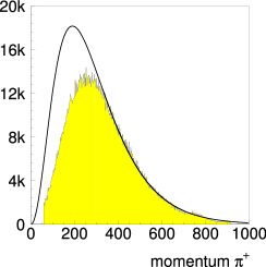
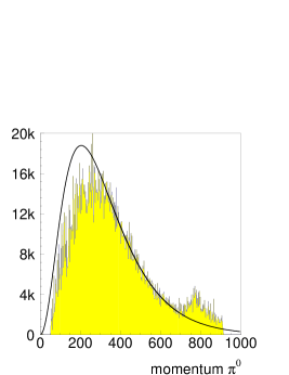
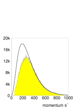
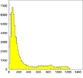
The inclusive momentum spectrum of charged particles (mostly pions) is shown in Fig. 12. The data are from the Crystal Barrel collaboration. The distribution reveals no significant structure, except for $\rho\pi$ production which identifies itself as a peak at 773 MeV / c in the momentum distribution. The $\rho^{0}$ signal seems much more pronounced; this is an artefact of the experimental resolution which is better for the recoiling $\pi^{0}$ than for $\pi^{\pm}$ mesons.

The absence of narrow signals in the momentum spectrum – which would indicate production of narrow quasinuclear bound states – is evident. Experiments in the early phase of LEAR confirmed the absence of narrow states against which charged or neutral pions would recoil [111, 265, 266].

Figure 12: The momentum distribution of charged and neutral pions.

From the number of events in Fig. 12 and the number of annihilation events, the average multiplicities

$$n_{\pi}=5.19\pm 0.15~{},\qquad n_{\pi^{\pm}}=3.12\pm 0.12~{},\qquad n_{\pi^{0}}=2.07\pm 0.08~{},$$ (5.5)

are found, consistent with those given in Eqs. (5.2) and (5.3).

The fit in Fig. 12 corresponds to a Maxwell–Boltzmann momentum distribution as proposed by Orfanidis and Rittenberg [267]. In the high-momentum range the fit follows the experimental distribution adequately thus defining a temperature of about 120 MeV. There is a mismatch at low momenta which is more pronounced for charged than for neutral pions. This is not due to a reduced efficiency of the detector for low momentum particles. Otherwise, the frequencies (5.5) would be smaller than those in (5.2) and (5.3); rather, pions at low momenta do not follow a simple thermal distribution law.

The temperature of 120 MeV should not be interpreted as an annihilation temperature, nor its inverse as an annihilation range of 1.7 fm. Pion interferometry gives a similar range; we will discuss the reasons for this wide range below.

5.3 Pion interferometry

In the fireball picture of $\bar{\mathrm{p}}$p annihilation, pions are emitted stochastically from an extended source. It can be argued that the pion fields emitted from different space-time points 1 and 2 superpose and interfere. The probability to detect a pion is then given by

$$dP_{12}\propto dr_{1}dr_{2}\,\left|e^{\displaystyle i[p_{1}(x_{1}-r_{1})+p_{2}(x_{2}-r_{2})]}+e^{\displaystyle i[p_{1}(x_{1}-r_{2})+p_{2}(x_{2}-r_{1})]}\right|^{2}~{}.$$ (5.6)

It is worthwhile to recall that such interferences were first used in astronomy, by Hanbury-Brown and Twiss (HBT) [268], to determine the diameter of Sirius from a measurement of the correlated intensity fluctuations in two optical telescopes. G. and S. Goldhaber, Lee and Pais [269] applied the effect to estimate the size in space–time of the source emitting pions in $\bar{\mathrm{p}}$p annihilation.

Different correlation signals have been defined to extract the correlation between pions due to the HBT effect. We mention here the two-pion correlation function

$$C(p_{1},p_{2})=\frac{\rho_{2}(p_{1},p_{2})}{\rho_{0}(p_{1},p_{2})}\,,$$ (5.7)

where $\rho_{2}(p_{1},p_{2})$ represents the distribution of two mesons correlated due to the HBT effect, and $\rho_{2}(p_{1},p_{2})$ an uncorrelated sample. The uncorrelated distribution can be chosen as the product of two single particle distributions $\rho_{2}(p_{1},p_{2})=\rho_{1}(p_{1})\rho_{1}(p_{2})$, where

 

$${\rho_{1}(p_{i})}$$

  (5.8)

The correlated sample may be pion pairs of equal charge; for the uncorrelated pion pair, pions of different charge or from different events can be used.

In $\bar{\mathrm{p}}\mathrm{p}$ and $\bar{\mathrm{p}}\mathrm{d}$ annihilation, the HBT effect was used by different groups. The precise source parameters depend on the data (annihilation into $2\pi^{+}2\pi^{-}$ or $2\pi^{+}2\pi^{-}n\pi^{0}$) and the model (with unlike-sign pions or different events to determine the uncorrelated dipion spectrum). The results given in [270] and [120] are not compatible with each other within the quoted errors; the value for the Bose–Einstein correlation parameter,

$$r_{\rm BE}=c\tau_{\rm BE}=1.5\pm 0.3\,{\rm fm}\,,$$ (5.9)

seems to be a fair estimate of the dimension of the pion source in space and time. It corresponds approximately to the pion Compton wave length $\lambda_{\pi}$. Again, this is not the size of the annihilation source. Rather, it is the size of the source from which pions are emitted. Pions may be emitted as initial- or final-state radiation (even though there is no experimental support for these processes); but certainly, pions are produced in secondary decays over a wide range of distances. Equation (5.9) indicates that interference between pions is strong for distances corresponding to $\lambda_{\pi}$. This is a trivial statement as long as the annihilation range is small compared to $\lambda_{\pi}$.

The result (5.9) is in rather strong disagreement with recent findings by Locher and Markushin using CPLEAR [271, 272] and Crystal Barrel [273] data. These authors go beyond the conventional HBT analysis by plotting the double-differential cross-sections as a function of the invariant masses $M_{++}$ and $M_{--}$, where the sign stands for the charge of the dipion. In a first article, devoted to $\bar{\mathrm{p}}\mathrm{p}\to 2\pi^{+}2\pi^{-}$, a source dimension of the order of 0.4 fm is quoted, in fair agreement with the value we will derive in Sec. 8 from the systematics of two-body annihilation frequencies. Locher and Markushin warn the reader that the interpretation of the observed correlation signal by the conventional HBT effect is questionable. They observe strong enhancements at low values of $M_{++}$ and $M_{--}$, and notice that the signal for pion pairs of large momenta ($\sim 800$ MeV/c) – which should be sensitive to the source dimension of 0.4 fm – gives a coherence which is unreasonably large within the HBT framework. In the analysis of the $\bar{\mathrm{p}}\mathrm{p}\to 2\pi^{+}2\pi^{-}\pi^{0}$ reaction, they show that the enhancement at low values of $M_{++}$ and $M_{--}$ can be simulated as the effect of the trivial need to symmetrise isobar amplitudes. Best suited is an interference between $\rho\sigma\pi$ and $\rho\rho\pi$ amplitudes. Such an ansatz reproduces also the momentum dependence of the correlation signal. The author thus refuse to provide simple numbers on the size and life time of the hypothetical $\bar{\mathrm{p}}\mathrm{p}$ fire-ball. Also in the case of the reaction $\bar{\mathrm{p}}\mathrm{p}\to 4\pi^{0}$, an interpretation within the conventional isobar model is possible, and there is no evidence for an additional signal due to the HBT effect. It may be worthwhile to recall that the HBT effect has not been taken into account explicitly in partial-wave analyses of bubble-chamber or LEAR data; it is only partly accounted for by Bose–Einstein symmetrisation of the amplitudes. There is no parameter to describe the source dimension.

5.4 Strangeness production

The full data sets at BNL and CERN were scanned in searches for $\mathrm{K_{s}}$ decays into $\pi^{+}\pi^{-}$, leading to secondary vertices. These data samples comprised 40,000 and 20,000 events, respectively, with strange particles in the final state. In the presence of one $\mathrm{K_{s}}$, the ionisation density of the tracks was used to identify the charged-kaon track. Table 9 gives annihilation frequencies with an observed $\mathrm{K_{s}}$.

Table 9: Frequencies of $\bar{\mathrm{p}}\mathrm{p}$ annihilation at rest in liquid H₂ into kaonic final states (in units of $10^{-3}$) from [2]. The data are corrected for unseen decay modes of the $\mathrm{K_{s}}$ and for the $\mathrm{K_{s}}$ reconstruction efficiency. $\mathrm{K}^{0}$ stands for the sum of $\mathrm{K_{s}}$ and $\mathrm{K_{l}}$. For the derivation of the $\mathrm{K_{s}}\mathrm{K_{l}}\pi^{0}$ frequency see [215].

Final state	BNL	CERN
$\mathrm{K}^{+}\mathrm{K}^{-}$	$1.10\pm 0.10$	$0.96\pm 0.08$
$\mathrm{K_{s}}\mathrm{K_{s}}+\mathrm{K_{l}}\mathrm{K_{l}}$	$0.010^{+0.012}_{-0.010}$	$0.008\pm 0.008$
$\mathrm{K_{s}}\mathrm{K_{l}}$	$0.71\pm 0.10$	$0.80\pm 0.05$
$(\mathrm{K_{s}}\mathrm{K_{s}}+\mathrm{K_{l}}\mathrm{K_{l}})\pi^{0}$	$1.46\pm 0.20$	$1.56\pm 0.12$
$\mathrm{K_{s}}\mathrm{K_{l}}\pi^{0}$	$0.67\pm 0.07$	$0.67\pm 0.07$
$(\mathrm{K_{s}}\mathrm{K_{s}}+\mathrm{K_{l}}\mathrm{K_{l}})$MM	$1.28\pm 0.16$	$1.42\pm 0.26$
$\mathrm{K_{s}}\mathrm{K}^{\pm}\pi^{\mp}$	$4.25\pm 0.55$	$4.25\pm 0.20$
$(\mathrm{K_{s}}\mathrm{K_{s}}+\mathrm{K_{l}}\mathrm{K_{l}})\pi^{-}\pi^{+}$	$4.02\pm 0.52$	$3.90\pm 0.46$
$\mathrm{K_{s}}\mathrm{K_{l}}\pi^{-}\pi^{+}$	$2.41\pm 0.36$	$2.26\pm 0.45$
$\mathrm{K}^{0}\mathrm{K}^{\pm}\pi^{\mp}\pi^{0}$	$8.94\pm 1.06$	$9.38\pm 1.10$
$(\mathrm{K_{s}}\mathrm{K_{s}}+\mathrm{K_{l}}\mathrm{K_{l}})\pi^{-}\pi^{+}\pi^{0}$	$2.98\pm 0.44$	$2.20\pm 0.28$
$\mathrm{K}^{0}\mathrm{K}^{\pm}\pi^{\mp}\pi^{-}\pi^{+}$	$0.59\pm 0.08$	$0.71\pm 0.07$
$\mathrm{K}^{0}\mathrm{K}^{\pm}4\pi$	$\sim 0$	$\sim 0$
Sum	$28.4\pm 1.5$	$28.1\pm 1.4$

From Table 9 the fraction of events with at least one neutral $\mathrm{K_{s}}$ is determined to be

$$\mathrm{BR}(\bar{\mathrm{p}}\mathrm{p}\to\mathrm{K_{s}}+{\rm anything})=(1.55\pm 0.06)\%\,.$$ (5.10)

The rate for $\mathrm{K_{l}}$ production is obviously the same. The total yield of strange particle production has to include final states with $\mathrm{K}^{+}\mathrm{K}^{-}$ pairs. Based on a scan searching for high ionisation-density tracks, Armenteros et al. found a contribution of $(6.82\pm 0.25)$% to $\bar{\mathrm{p}}\mathrm{p}$ annihilation. In the CERN list of pionic annihilation modes, these events are included in the missing mass class of events. The BNL group assigns $(4.6\pm 1.8)$% of all annihilations to strangeness production, which agrees with the estimate $(4.74\pm 0.22)$% of Batusov [274] assuming that annihilation frequencies for $\bar{\mathrm{p}}\mathrm{p}\to\mathrm{K}^{+}\mathrm{K}^{-}n\pi$ are similar to those into $\mathrm{K}^{0}\overline{\mathrm{K}}{}^{0}n\pi$. A statistical treatment of these three numbers being not plausible, we quote here their linear mean and spread

$$\mathrm{BR}(\bar{\mathrm{p}}\mathrm{p}\to{\rm kaons}+{\rm anything})=(5.4\pm 1.7)\%\,.$$ (5.11)

In short, one event out of 20 contains strange particles in the final state.

5.5 Annihilation on neutrons

Antiproton–neutron or antineutron–proton interactions at rest offer additional opportunities to study annihilation dynamics. Obviously, both systems have isospin $I=1$. Under the hypothesis that annihilation at rest takes place when the $\overline{\mathrm{N}}\mathrm{N}$ system is in S-wave, $G$-parity fixes the total spin: a triplet $S=1$ has $G=(-1)^{L+S+I}=+1$ and leads to an even number of pions, while the spin singlet system gives an odd number of pions.

Since there exists no free-neutron target, the cleanest way to study pure isovector annihilation is to build a antineutron beam line (produced by charge exchange $\bar{\mathrm{p}}\mathrm{p}\to\bar{\mathrm{n}}\mathrm{n}$) at very low energies. The Obelix collaboration has made extensive use of this possibility [11] to study specific reactions as a function of the $\bar{\mathrm{n}}$ beam momentum. These results will be presented in Sec. 6. The topological annihilation frequencies agree within errors with those for $\bar{\mathrm{p}}\mathrm{n}$ [275] even though in the latter case, one has to worry about the role of the proton or neutron surviving the annihilation process. Global features of annihilation were derived by use of a deuterium target.

Naively, it may be expected that $\bar{\mathrm{p}}\mathrm{n}$ annihilation on a deuteron can be viewed at as two-step process:

$$\bar{\mathrm{p}}\mathrm{d}\to(\bar{\mathrm{p}}\mathrm{n})+\mathrm{p}~{},\qquad{\rm or}\qquad\bar{\mathrm{p}}\mathrm{d}\to\bar{\mathrm{p}}\mathrm{p}+\mathrm{n}~{},$$ (5.12)

with subsequent annihilation of the $\bar{\mathrm{p}}\mathrm{n}$ or $\bar{\mathrm{p}}\mathrm{p}$ system. This is, however, a crude approximation. Figure 13 shows the neutron momentum distribution for the reaction $\bar{\mathrm{p}}\mathrm{d}\to\mathrm{n}2\pi^{0}$ from the Crystal Barrel experiment [177].

Figure 13: Left: Neutron momentum distribution; right: p$\pi^{0}$ invariant mass distribution from the reaction $\rm\bar{p}d\to n2\pi^{0}$.

The neutron momentum distribution does not follow the Hulthén function. There is a significant excess of high-momentum neutrons. The reason can be understood once the p$\pi^{0}$ invariant mass is plotted, see Fig. 13, right. Baryon resonances are produced, e.g., in the reaction

$$\bar{\mathrm{p}}\mathrm{d}\to\Delta^{0}\pi^{0};\ \Delta^{0}\to\mathrm{n}\pi^{0}~{}.$$ (5.13)

This annihilation mode is called a Pontecorvo reaction; the surviving nucleon, proton or neutron, can be produced at a rather high momentum. In this case, a high-momentum $\Delta(1232)$ is produced. The systematics of Pontecorvo reactions will be discussed in Sec. 6.7.3.

In the low-momentum part in Fig. 13, the neutron has acquired little momentum; it acted as a spectator and was not involved in the annihilation process. A cut on this momentum, at 200 to 250 MeV/c in the analysis of bubble chamber data or at about 100 MeV/c in data taken at LEAR, makes sure that the annihilation took place on a quasi-free nucleon.

In bubble chambers, antiprotons annihilating on neutrons lead to odd numbers of visible pion tracks; the tracks of ’spectator’ protons with very low momenta (less than 80 MeV/c) are not separable from the primary ionisation spot produced by the stopped antiproton. Protons with momenta up to 250  MeV/c are easily identified by their large ionisation losses. Thus it was easy to separate annihilations on quasi-free protons and neutrons. Bizzarri [81] deduced probabilities $s_{\rm p}=0.571\pm 0.005$ and $s_{\rm n}=0.429\pm 0.005$ for annihilation on protons and neutrons, respectively. Antiprotons stopped in liquid D₂ annihilate more often on protons than on neutrons, with the ratio

$$s_{\rm p}/s_{\rm n}=1.331\pm 0.019~{}.$$ (5.14)

If the isospin content is denoted

$$s_{\mathrm{p}}=s_{\mathrm{p}}^{0}+s_{\mathrm{p}}^{1}~{},\quad s_{\mathrm{n}}=s_{\mathrm{n}}^{1}~{},$$ (5.15)

we have $s_{p}^{1}=s_{\mathrm{n}}^{1}/2$, thus ensuring model-independent relations due to overall isospin conservation, such as

$$\frac{\mathrm{BR}(\bar{\mathrm{p}}\mathrm{d}\to\pi^{-}\omega\mathrm{p})}{\mathrm{BR}(\bar{\mathrm{p}}\mathrm{d}\to\pi^{0}\omega\mathrm{n})}=2~{}.$$ (5.16)

Then $s_{\mathrm{p}}^{0}>s_{\mathrm{p}}^{1}$, more precisely, $s_{\mathrm{p}}^{0}=(1.662\pm 0.038)\,s_{\mathrm{p}}^{1}$, is needed to get the observed $s_{\rm p}/s_{\rm n}$. This means that in $\mathrm{D}_{2}$, isoscalar $\bar{\mathrm{p}}\mathrm{p}$ annihilation is significantly more frequent than isovector annihilation.

Table 10 lists the global annihilation frequencies for $\bar{\mathrm{p}}\mathrm{d}$ annihilation into pions and kaons for events with spectator protons. Frequencies for final states with more than one $\pi^{0}$ are from [209, 216] the frequency for $\bar{\mathrm{p}}\mathrm{n}\to\pi^{-}\pi^{0}$ is derived in [209, 276]. The Crystal Barrel collaboration [209, 216] used no spectator cut to determine frequencies.

Table 10: Frequencies of $\bar{\mathrm{p}}\mathrm{n}$ annihilation at rest in liquid D₂ into pionic final states [78] and into final states with strangeness [79] after a cut on the spectator momentum of the proton at 250 MeV/c .

Final state Frequency (in%) $\pi^{-}n\pi^{0}$ $16.4\pm 0.5$    $\pi^{-}\pi^{0}$ $0.40\pm 0.04$    $\pi^{-}2\pi^{0}$ $0.68\pm 0.07$    $\pi^{-}4\pi^{0}$ $1.32\pm 0.20$ $2\pi^{-}\pi^{+}n\pi^{0}$ $59.7\pm 1.2$    $2\pi^{-}\pi^{+}$ $1.57\pm 0.21$    $2\pi^{-}\pi^{+}\pi^{0}$ $21.8\pm 2.2$    $2\pi^{-}\pi^{+}2\pi^{0}$ $7.0\pm 1.1$ $3\pi^{-}2\pi^{+}n\pi^{0}$ $23.4\pm 0.7$    $3\pi^{-}2\pi^{+}$ $5.15\pm 0.47$    $3\pi^{-}2\pi^{+}\pi^{0}$ $15.1\pm 1.0$ $4\pi^{-}3\pi^{+}n\pi^{0}$ $0.39\pm 0.07$ Sum $95.5\pm 1.5$%

Final state Frequency (in $10^{-4}$) $\mathrm{K}^{0}\mathrm{K}^{-}$ $14.7\pm 2.1$ $\mathrm{K}^{0}\mathrm{K}^{-}\pi^{0}$ $36.0\pm 4.2$ $\mathrm{K_{s}}\mathrm{K_{s}}\pi^{-}$ $14.7\pm 2.0$ $\mathrm{K_{s}}\mathrm{K}_{l}\pi^{-}$ $21.2\pm 3.6$ $\mathrm{K}^{0}\mathrm{K}^{+}\pi^{-}\pi^{-}$ $24.8\pm 2.6$ $\mathrm{K}^{0}\mathrm{K}^{-}\pi^{+}\pi^{-}$ $34.2\pm 3.5$ $\mathrm{K_{s}}\mathrm{K_{s}}\pi^{-}\pi^{0}$ $25.6\pm 2.8$ $\mathrm{K}^{0}\mathrm{K}^{+}\pi^{-}\pi^{-}\pi^{0}$ $1.6\pm 0.9$ $\mathrm{K_{s}}\mathrm{K}^{-}\pi^{+}\pi^{-}\pi^{0}$ $33.6\pm 3.8$ $\mathrm{K_{s}}\mathrm{K}^{-}\omega$ $35.0\pm 5.2$ $\mathrm{K_{s}}\mathrm{K_{s}}\pi^{+}\pi^{-}\pi^{-}$ $2.8\pm 1.2$ $\mathrm{K_{s}}\mathrm{K_{l}}\pi^{+}\pi^{-}\pi^{-}$ $1.9\pm 1.2$ Sum $2.5\pm 0.1$%

6 Annihilation into two mesons

6.1 Introduction

The study of $\overline{\mathrm{N}}\mathrm{N}$ annihilation at rest into two mesons is a rich source of information about annihilation dynamics. The role of symmetries, the topology of the dominant quark diagrams, the violation of the Zweig rule, etc., can be inferred from the knowledge of the two-meson frequencies. Detailed information on the density dependence of annihilation frequencies is required if these frequencies are to be assigned to specific states of the $\bar{\mathrm{p}}\mathrm{p}$ or $\bar{\mathrm{p}}\mathrm{d}$ atom. This arises from the sensitivity of two-meson annihilation to the initial state of the nucleon-antinucleon system. For example, from Table 5, we see that the process $\bar{\mathrm{p}}\mathrm{p}\rightarrow\pi^{+}\pi^{-}$ takes place from initial S- and P- states whilst the reaction $\bar{\mathrm{p}}\mathrm{p}\rightarrow\pi^{0}\pi^{0}$ only originates from P-states. At first glance, it would seem that the fraction of P-state annihilation could be obtained from the relevant $\pi^{+}\pi^{-}$ and $\pi^{0}$$\pi^{0}$ annihilation frequencies using isospin invariance and simple arithmetic. The derivation of the P-state fraction is actually more subtle and unfortunately, more complex. In particular it depends on details of the atomic cascade process and on the amount of Stark mixing. On the other hand, a thorough analysis of these cascade effects enables us to obtain the fraction of $\bar{\mathrm{p}}\mathrm{p}$ annihilation into a variety of channels from different fine-structure states of the $\bar{\mathrm{p}}\mathrm{p}$ system. The information which is directly given by the $\pi^{+}\pi^{-}$ and $\pi^{0}$$\pi^{0}$ frequencies is the fraction of annihilations for the $\pi^{+}\pi^{-}$ and $\pi^{0}$$\pi^{0}$ channels which take place from S- and P-states. This is not the same as the fraction of S- and P-state annihilations for the $\bar{\mathrm{p}}\mathrm{p}$ system.

We first start with a few definitions. The annihilation frequency $\mathrm{AF}(ch,\rho$), often also called the branching ratio in the literature, is the probability that a particular channel $ch$ will be produced in a $\bar{\mathrm{p}}\mathrm{p}$ or $\bar{\mathrm{p}}\mathrm{d}$ annihilation at rest. It is usually the quantity measured experimentally and is a function of the target density $\rho$. We restrict the term branching ratio $\mathrm{BR}(ch,{}^{2S+1}L_{J}$) to the probability that the channel $ch$ is produced by an annihilation from the initial state ${}^{2S+1}L_{J}$ of the $\bar{\mathrm{p}}\mathrm{p}$ or $\bar{\mathrm{p}}\mathrm{d}$ atom. These branching ratios are independent of the atomic physics effects occurring during the cascade of the $\bar{\mathrm{p}}\mathrm{p}$ or $\bar{\mathrm{p}}\mathrm{d}$ atom and hence do not depend on the target density. It is this quantity which normally should be compared with predictions from theoretical models. In Sec. 7, we shall define dynamically corrected branching ratios, DR, including phase space corrections, orbital-angular-momentum-barrier effects, and a phenomenological factor favouring the production of high-mass mesons.

Many of the earlier experiments measured two-body annihilation frequencies by the detection and reconstruction of a single $\pi^{0}$ or $\eta$ with a small solid-angle detector and observed peaks in the resulting $\pi^{0}$ or $\eta$ inclusive momentum spectrum to identify the second meson (see Table 3). Since the annihilation frequencies are small, these early data are often statistically weak or subject to very considerable uncertainties in the background subtraction from the inclusive spectra. In more recent experiments, using detectors covering a large solid angle, both of the mesons in the two-body events are fully reconstructed and any background is much reduced.

At a given target density $\rho$, the annihilation frequency for the channel $ch$ is given by

$$\mathrm{AF}(ch)=\frac{N_{evts}(ch)}{N_{tot}\epsilon_{det}VF_{1}F_{2}}~{},$$ (6.1)

where $\epsilon_{det}$ is the detection efficiency given by

$$\epsilon_{det}=\frac{N^{MC}_{evts}(ch)}{N^{MC}_{tot}}~{}.$$ (6.2)

$N_{tot}$ is the total number of antiprotons stopped in the target, corrected for pile-up, and $N_{evts}(ch)$ is the number of events, corrected for background, attributed to channel $ch$. $N^{MC}_{tot}$ and $N^{MC}_{evts}(ch)$ are the corresponding numbers for the Monte-Carlo simulation and reconstruction. $V$ is the fraction of antiproton events which stop in the target volume and $F_{1}$ and $F_{2}$ are the correction factors for the probability of the observed decay for each of the two mesons in channel $ch$; for example $F=0.3943\pm 0.0026$ for $\eta\ \rightarrow\ 2\gamma$ in the case where the two photons are measured so as to reconstruct the $\eta$ meson.

Here we will particularly discuss two-body annihilation frequencies for channels involving narrow ($\Gamma\ \leq$ 10 MeV) mesons ($\pi,\mathrm{K},\eta,\ \eta^{\prime},\ \omega$ and $\phi$). Measurements of annihilation frequencies for broader states from inclusive spectra usually have considerable uncertainties due to the need for background subtraction. In addition, reflections can distort the spectrum in an unpredictable way. For measurements of two-body annihilation frequencies of broad states a full partial wave analysis involving all intermediate states is required. For completeness, we include two-body branching ratios involving the K^∗ ($\Gamma$ = 50 MeV) and $\rho$ ($\Gamma$ = 151 MeV) mesons. Some two-meson annihilation frequencies obtained from partial wave analyses involving pseudovector or tensor mesons are also discussed.

In measurements of frequencies for two-body annihilation from $\bar{\mathrm{p}}\mathrm{p}$ atoms, the selection of events is straightforward, requiring just two back-to-back particles each of the same well-defined momentum. For $\bar{\mathrm{p}}\mathrm{d}$ atoms the selection is less straightforward due to the presence of the recoil nucleon which, in some cases, can have momenta up to 1.2 $\,{\mathrm{Ge\hskip-1.0ptV}\hskip-2.0pt/\hskip-1.0ptc}$ [84, 209]. Measurement of their frequencies requires that all events over the full range of spectator momenta are included. An additional effect is that the spectator momentum distribution depends [84] on whether the annihilation occurs from an atomic S- or P-state of the $\bar{\mathrm{p}}\mathrm{d}$ system and whether the $\bar{\mathrm{p}}$ is in an S- or P-state relative to the nucleon with which it annihilates. In particular the momentum distribution for P-state $\bar{\mathrm{p}}$N annihilation from an atomic S-state is particularly broad. It was pointed out [277] that tight cuts on the momentum of the spectator nucleon therefore suppresses P-state annihilation from atomic S-state orbitals.

For $\bar{\mathrm{p}}\mathrm{d}$ annihilations at rest, the annihilation frequency is determined by normalising either to the total number of annihilations on a deuteron or to the number of annihilations on a proton or neutron. In the following, subscripts d and N (p or n), will be used to distinguish between frequencies measured for annihilation on deuterons or on a nucleon (proton or neutron) in the deuteron. Sometimes, it has been assumed that there is equal probability for annihilation on a proton or neutron in the deuteron. In this case the branching ratio for $\bar{\mathrm{p}}\mathrm{d}$ annihilation would be obtained simply by dividing by a factor of two. Here, we use the probabilities $s_{\rm p}=0.571\pm 0.005$ and $s_{\rm n}=0.429\pm 0.005$ deduced by Bizzarri [81], as discussed already in Sec. 5.5. The annihilation frequency on a deuteron, for reactions involving a spectator neutron, is then given by

$$\mathrm{AF}_{\rm d}(ch,{\rm n},\rho)=s_{\rm p}\mathrm{AF}_{\rm p}(ch,{\rm n},\rho)\,,$$ (6.3)

and similarly for reactions involving a spectator proton.

In Sec. 6.2, we discuss the $\bar{\mathrm{p}}\mathrm{p}$ and $\bar{\mathrm{p}}\mathrm{d}$ atomic cascade, the effects of Stark mixing, the role of the fine-structure levels and the need for enhancement factors. Atomic cascade calculations, and in particular the prediction of enhancement factors is discussed in Sec. 6.3 for both $\bar{\mathrm{p}}\mathrm{p}$ and $\bar{\mathrm{p}}\mathrm{d}$ atoms. Published annihilation frequencies for $\bar{\mathrm{p}}\mathrm{p}$ atoms are reviewed in Sec. 6.4 which also contains a detailed discussion of the $\bar{\mathrm{p}}\mathrm{p}$$\to$$\pi^{0}$$\pi^{0}$ annihilation frequency. A new analysis of two-body annihilation frequencies for $\bar{\mathrm{p}}\mathrm{p}$ atoms is presented in Sec. 6.5 with an emphasis on determining the fraction of P-state annihilation and branching ratios for annihilation from specific atomic states. Section 6.6 reviews antineutron annihilation on protons whilst section 6.7.1 reviews annihilation frequencies from $\bar{\mathrm{p}}\mathrm{d}$. The determination of the P- state fraction in $\bar{\mathrm{p}}\mathrm{d}$ annihilation is presented in Sec. 6.7.2. A compilation of data on Pontecorvo reactions is given in Sec. 6.7.3. Some final remarks on aspects of two-meson annihilation are made in Sec. 6.8.

6.2 Stark mixing and density dependence of annihilation frequencies

6.2.1 $\bar{\mathrm{p}}\mathrm{p}$ atoms

Formation of the $\bar{\mathrm{p}}\mathrm{p}$ atom and its atomic cascade has been discussed in the earlier review [1] and elsewhere [278, 279]. Briefly, the capture of the $\bar{\mathrm{p}}$ typically occurs at a principal quantum number $n\approx 30$ [280]. De-excitation then takes place by a number of processes including radiative transitions with the emission of X-rays, and the external Auger effect involving the ionisation of a neighbouring $\mathrm{H}_{2}$ molecule. Finally the $\bar{\mathrm{p}}$ reaches an atomic state with angular momentum $L=0$ or 1 when annihilation occurs. Annihilation from states with $L\geq 2$ can be ignored due to the negligible overlap of $\bar{\mathrm{p}}$ and p in the atomic wavefunction.

In addition, except at very low target densities, the Stark effect gives mixing of the angular momentum states $L$ at high $n$ allowing the protonium atoms to transfer to S- and P-states where they can annihilate before reaching the low-$n$ states. The Stark mixing increases with the target density; for liquid targets the rate is very high. When considering frequencies for $\bar{\mathrm{p}}\mathrm{p}$ annihilation, it is important to consider the effects of the fine-structure of the atomic states. For $\bar{\mathrm{p}}\mathrm{p}$ atoms, the states with $L<2$ are ${}^{1}{{\mathrm{S}}}_{0}$, ${}^{3}{{\mathrm{S}}}_{1}$, ${}^{1}{{\mathrm{P}}}_{1}$, ${}^{3}{{\mathrm{P}}}_{0}$, ${}^{3}{{\mathrm{P}}}_{1}$ and ${}^{3}{{\mathrm{P}}}_{2}$ with the corresponding $J^{PC}$= $0^{-+}$, $1^{--}$, $1^{+-}$, $0^{++}$, $1^{++}$ and $2^{++}$. Table 11 shows the predictions of Carbonell et al.[259] for the widths of these states. They were obtained using potentials for the $\bar{\mathrm{p}}\mathrm{p}$ interaction due to Dover and Richard (DR1 and DR2) and Kohno and Weise (KW). A particular feature of these predictions is the very large width of the ${}^{3}{{\mathrm{P}}}_{0}$ state which has been confirmed in recent experiments. Gotta et al [281], assuming the widths of the ${}^{1}{{\mathrm{P}}}_{1}$, ${}^{3}{{\mathrm{P}}}_{1}$ and ${}^{3}{{\mathrm{P}}}_{2}$ states to be equal, obtain $\Gamma({}^{3}{{\mathrm{P}}}_{0})=120\pm 25$ meV and $\Gamma({}^{1}{{\mathrm{P}}}_{1},{}^{3}{{\mathrm{P}}}_{1},{}^{3}{{\mathrm{P}}}_{2})=30.5\pm 2.8$ meV for the states with principal quantum number $n=2$, in good agreement with the values listed in Table 11. The average value of the width of the 1S state given by four experiments is quoted in the earlier review [1] as $\Gamma(1\mbox{S})=1.060\pm 0.080$ keV which again is in good agreement with the values of Table 11.

Table 11: Widths for $\bar{\mathrm{p}}\mathrm{p}$ atoms as predicted by three potential models

State	${}^{1}{{\mathrm{S}}}_{0}$	${}^{3}{{\mathrm{S}}}_{1}$	${}^{1}{{\mathrm{P}}}_{1}$	${}^{3}{{\mathrm{P}}}_{0}$	${}^{3}{{\mathrm{P}}}_{1}$	${}^{3}{{\mathrm{P}}}_{2}$
Units	keV	keV	meV	meV	meV	meV
DR1	1.02	0.90	26	114	20	30
DR2	1.04	0.92	28	80	18	32
KW	1.26	0.98	26	96	22	36

At high $n$, in the case where Stark mixing is important, the fine-structure levels are continually and rapidly repopulated according to their statistical weight. A fine structure level with a large annihilation width will therefore contribute more to annihilation than would be expected from its statistical weight only. This effect is particularly important for the ${}^{3}{{\mathrm{P}}}_{0}$ level. Similar, but smaller, effects will also occur for the other fine structure P-states. The effects for S-states are typically less than 5 %.

These deviations of the population of the fine-structure states have been described [282] in terms of enhancement factors $E({}^{2S+1}L_{J},\rho)$ which are functions of the initial state ${}^{2S+1}L_{J}$ and target density $\rho$. Values of $E({}^{2S+1}L_{J},\rho)<1\ (>1)$ correspond to a fraction of annihilations smaller (larger) than that expected on the basis of a purely statistical population of the level.

The annihilation frequency $\mathrm{AF}(ch,\rho)$ can then be written [282] in terms of the branching ratios $\mathrm{BR}$($ch,{}^{2S+1}L_{J}$) in the form

 

$${\mathrm{AF}(ch,\rho)=\left(1-\mathrm{f}_{\rm{P}}(\rho)\right)\Bigl{[}}$$

  (6.4)

where $\mathrm{f}_{\rm{P}}(\rho)$ is the fraction of P-state annihilation and the factors 1/4, 5/12, etc., are the statistical weights of the states. In those cases where production of the channel $ch$ is forbidden from an initial state ${}^{2S+1}L_{J}$ due to selection rules, then $\mathrm{BR}(ch,{}^{2S+1}L_{J})=0$.

The enhancement factors are normalised [282] so that

$$\frac{1}{4}E({}^{1}{{\mathrm{S}}}_{0},\rho)+\frac{3}{4}E({}^{3}{{\mathrm{S}}}_{1},\rho)=1~{},$$ (6.5)

and

$$\frac{3}{12}E({}^{1}{{\mathrm{P}}}_{1},\rho)+\frac{1}{12}E({}^{3}{{\mathrm{P}}}_{0},\rho)+\frac{3}{12}E({}^{3}{{\mathrm{P}}}_{1},\rho)+\frac{5}{12}E({}^{3}{{\mathrm{P}}}_{2},\rho)=1~{}.$$ (6.6)

From Eq. (6.4) it can be seen that the density dependence of $\mathrm{AF}(ch,\rho)$ arises from two factors. The first and larger one is the density dependence of the fraction of P-state annihilation, $\mathrm{f}_{\rm{P}}(\rho)$, which is directly due to the Stark effect. The second and more subtle one arises from the enhancement factors $E({}^{2S+1}L_{J},\rho)$. In cases where these differ significantly at a given $\rho$ for various ${}^{2S+1}L_{J}$, the branching ratios for these states, $\mathrm{BR}(ch,{}^{2S+1}L_{J})$ can be determined.

Attempts have been made to determine the values of the enhancement factors from experimental data. A study [198] of the reaction $\bar{\mathrm{p}}\mathrm{p}\rightarrow\eta\pi^{0}\pi^{0}\pi^{0}$ at rest, both in liquid and in gas at 12 $\rho_{\rm{STP}}$, where STP indicates Standard Temperature and Pressure, finds

$$r=\frac{E({}^{3}{{\mathrm{P}}}_{0},{\rm liq.})/E({}^{3}{{\mathrm{P}}}_{0},12\ \rho_{\rm{STP}})}{E({}^{3}{{\mathrm{P}}}_{2},{\rm liq.})/E({}^{3}{{\mathrm{P}}}_{2},12\ \rho_{\rm{STP}})}=2.46\pm 0.15~{},$$ (6.7)

to be compared with the value $r\approx\ 1.7$ obtained using predicted values for the enhancement factors from Table 12 which will be discussed later.

Salvini et al. [283] have attempted to determine enhancement factors directly from a best fit to two-body annihilation frequencies. The fit procedure was not straightforward since they obtained different local minima with more or less equivalent $\chi^{2}$ values. This is probably due to the fact that the values of $\mathrm{BR}(ch,{}^{2S+1}L_{J})$ and $E({}^{2S+1}L_{J},\rho)$ are strongly correlated, appearing in the form $E({}^{2S+1}L_{J},\rho)\mathrm{BR}(ch,{}^{2S+1}L_{J})$ in Eq. (6.4). The solutions were constrained to those that were regarded as physically meaningful, the remaining parameter space was explored in detail. In most cases values for $E({}^{2S+1}L_{J},\rho)$ were obtained consistent with unity except for $E({}^{3}{{\mathrm{P}}}_{0},{\rm liq.})$ which was in the range $1.7\pm 0.3$ to $3.6\pm 0.1$, depending on the value for $\mathrm{AF}(\pi^{0}\pi^{0},{\rm liq})$ used in the data analysis. The discrepancies between the different experimental values for the $\bar{\mathrm{p}}\mathrm{p}\rightarrow\pi^{0}\pi^{0}$ annihilation frequency in liquid $\mathrm{H}_{2}$ will be discussed in Sec. 6.4.3.

More recently Bargiotti et al. [284] have determined enhancement factors $E({}^{2S+1}L_{J},\rho)$ for all S- and P- fine-structure states in liquid and gas ($\rho_{\rm{STP}}$) targets by fitting measurements for two-body and and also for resonant two-body channels obtained from partial wave analyses of the channels $\pi^{+}\pi^{-}\pi^{0}$, $\mathrm{K}^{\pm}\mathrm{K}^{0}_{\rm s}\pi^{\mp}$ and $\mathrm{K}^{+}\mathrm{K}^{-}\pi^{0}$ in hydrogen targets at three different densities $(\rho=0.005\rho_{\rm{STP}},$ $\rho_{\rm{STP}}$ and liquid). They fix the enhancement factors at low density $E({}^{2S+1}L_{J},0.005\rho_{\rm{STP}})=1$. With this assumption they were able to obtain a good fit to the measurements with enhancement factors different from one for the ${}^{1}{{\mathrm{P}}}_{1}$, ${}^{3}{{\mathrm{P}}}_{0}$ and ${}^{3}{{\mathrm{P}}}_{1}$ levels in liquid hydrogen . Comparison with the predictions of cascade calculations (see Table 12) shows good agreement for the ${}^{3}{{\mathrm{P}}}_{0}$ level but disagreement for the ${}^{1}{{\mathrm{P}}}_{1}$ and ${}^{3}{{\mathrm{P}}}_{1}$ levels with the ${}^{1}{{\mathrm{P}}}_{1}$ level, $E({}^{1}{{\mathrm{P}}}_{1},{\rm liq.})=0.09\pm 0.17$, being particularly strongly suppressed. The reason for this discrepancy is not understood.

An alternative approach [282] is to calculate values of $E({}^{2S+1}L_{J},\rho)$ using an atomic cascade calculation [278] for the $\bar{\mathrm{p}}\mathrm{p}$ atom whose parameters are obtained by fits to $\bar{\mathrm{p}}\mathrm{p}$ atomic X-ray data. This method will be discussed in detail in Sec. 6.3.

6.2.2 $\bar{\mathrm{p}}\mathrm{d}$ atoms

The general features of the atomic cascade for $\bar{\mathrm{p}}\mathrm{d}$ atoms are very similar to those for $\bar{\mathrm{p}}\mathrm{p}$ atoms discussed above, except that the $\bar{\mathrm{p}}$ is now captured at a principal quantum number $n\approx\ 45$ and that the much larger predicted widths [285] for the 2P levels in $\bar{\mathrm{p}}\mathrm{d}$ atoms give rise to increased probabilities for annihilation from atomic P-states. D-state annihilation also becomes significant. Wycech et al. [285] predict that the widths of the fine-structure components for P-states are approximately equal. It is therefore to be expected that for $\bar{\mathrm{p}}\mathrm{d}$ atoms the enhancement factors will have values $E({}^{2S+1}L_{J},\rho)\approx 1$ and their effect can be neglected.

Due to the Fermi motion of the nucleons in deuterium, the $\bar{\mathrm{p}}$-nucleon angular momentum can be different from the angular momentum of the $\bar{\mathrm{p}}$ with respect to the deuteron centre of mass. Even when the $\bar{\mathrm{p}}$ is in an atomic S-state, it may be in a P-state relative to the nucleon with which it annihilates. This process, sometimes called “induced” P-state annihilation, was first considered by Bizzarri et al. [84] and has recently been discussed by Bugg [286]. It is an assumption of these models that the antiproton interacts with only one of the two nucleons in the deuteron, the other behaving as a “spectator”. As a consequence, the annihilation frequencies in deuterium are directly related to the frequencies for capture on neutrons and protons. For the remainder of this article we use the following notation: capital letters denote the initial $\bar{\mathrm{p}}\mathrm{d}$ atomic states whilst the subscript “ann” (e.g., $\mathrm{P}_{\mathrm{ann}}$) is used to describe the annihilation process. This differs from the notation of Bugg [286], which was also used by Batty [287], where small letters denote the initial $\bar{\mathrm{p}}\mathrm{d}$ atomic states and capital letters were used to describe the annihilation process. For the $\bar{\mathrm{p}}\mathrm{p}$ system the fraction of annihilation from P-states of the $\bar{\mathrm{p}}\mathrm{p}$ atom $\mathrm{f}_{\rm{P}}(\rho)$, and the fraction of P-state $\bar{\mathrm{p}}\mathrm{p}$ annihilation $\mathrm{f}_{\rm{P}_{\rm{ann}}}(\rho)$ are, of course, the same.

6.3 Cascade calculations

6.3.1 $\bar{\mathrm{p}}\mathrm{p}$ atoms

In the calculations of enhancement factors [282], measurements of atomic X-ray yields for $\bar{\mathrm{p}}\mathrm{p}$ atoms, covering the range of target densities from 0.016 to 10.0 $\rho_{\rm{STP}}$, were analysed using a cascade calculation based on the method of Borie and Leon [288]. In this method the effects of Stark mixing are calculated using an impact parameter technique in which, in its interaction with the electric field of the neighbouring $\mathrm{H}_{2}$ molecules, the exotic atom is treated as moving along a straight line trajectory. If an atomic S-state is involved, the removal of the degeneracy due to the energy shift caused by the strong interaction hinders the Stark mixing, since the electric field must overcome the energy difference between S- and P-states. This is taken into account by using a smaller impact parameter. Because of the uncertainties in the absolute rate for Stark mixing, an overall normalisation parameter $k_{\rm STK}$ is usually used and its value determined by fitting the X-ray yields.

An alternative method, usually referred to as the “Mainz” model, has been developed in [289, 277]. Here the collisions of the $\bar{\mathrm{p}}\mathrm{p}$ atoms with the neighbouring $\mathrm{H}_{2}$ molecules are simulated using

Figure 14: Fraction of P-state annihilation predicted by the Borie–Leon model [288] giving a best fit to the X-ray data with $K_{0}=1$ (dashed line) or $K_{0}=7.6$ (full line). Also shown are the predictions of the Mainz [289, 277] model (dotted line) and the values derived in the present work from annihilation frequencies and annihilation widths from the DR1 potential

the classical-trajectory Monte-Carlo method which only allows Stark mixing when the $\bar{\mathrm{p}}\mathrm{p}$ atom experiences strong electric fields during collisions with neighbouring hydrogen molecules. This avoids the uncertainties associated with the straight line approximation used by Borie and Leon [288] at the expense of a considerable increase in computational complexity. Further information about cascade calculations is given in earlier reviews [1, 278].

Once the parameter $k_{\rm STK}$ in the Borie–Leon model has been adjusted to fit the X-ray data [282], the two models give similar predictions for the overall variation in the X-ray yields as a function of target density. However the Borie and Leon model predicts a significantly larger fraction for P-state annihilation in $\bar{\mathrm{p}}\mathrm{p}$ atoms than the “Mainz” model as shown in Fig. 14. It has been shown [282] that the introduction of an additional parameter $K_{0}$, as a further normalisation factor to the rate of Stark transitions between atomic S- and P-states, gives significantly improved fits to the X-ray yield data for $\bar{\mathrm{p}}\mathrm{p}$ atoms and much reduced values for the fraction of P-state annihilation in $\bar{\mathrm{p}}\mathrm{p}$ atoms. Setting $K_{0}$ = 1 gives the usual form of the Borie and Leon model.

Values of $E({}^{2S+1}L_{J},\rho)$ for P-states calculated [282] using the Borie–Leon cascade model with the DR1 annihilation widths of Table 11 are shown in Fig. 15. The corresponding enhancement factors for the S-states are generally close to 1. Table 12 gives numerical values for the enhancement factors, for all target pressures at which annihilation frequencies have been measured, for the three annihilation models of Table 11. The errors quoted are those due to the uncertainties in the parameters $K_{0}=7.6\pm 2.6,\ k_{\rm STK}=1.19\pm 0.06$ used to fit the X-ray yield data for $\bar{\mathrm{p}}\mathrm{p}$ atoms.

Figure 15: P-state enhancement factors from a cascade calculation [282] using $K_{0}=7.6$ and annihilation widths from the DR1 potential

Table 12: Calculated enhancement factors, as a function of the density $\rho$ (in units of $\rho_{\mathrm{STP}}$).

State	$\rho=0.002$	$\rho=0.005$	$\rho=1$	$\rho=12$	$\rho=15$	$\rho=27$	Liquid	Model
	1.044	1.046	1.020	1.011	1.012	1.013	1.032	DR1
	${}\pm 0.001$	${}\pm 0.001$	${}\pm 0.002$	${}\pm 0.001$	${}\pm 0.001$	${}\pm 0.001$	${}\pm 0.001$
${}^{1}{{\mathrm{S}}}_{0}$	0.973	0.975	1.007	1.005	1.005	1.007	1.028	DR2
	${}\pm 0.001$	${}\pm 0.001$	${}\pm 0.001$	${}\pm 0.001$	${}\pm 0.001$	${}\pm 0.001$	${}\pm 0.001$
	1.138	1.139	1.030	1.019	1.020	1.022	1.060	KW
	${}\pm 0.001$	${}\pm 0.001$	${}\pm 0.003$	${}\pm 0.001$	${}\pm 0.001$	${}\pm 0.001$	${}\pm 0.001$
	0.985	0.985	0.993	0.996	0.996	0.996	0.989	DR1
	${}\pm 0.001$	${}\pm 0.001$	${}\pm 0.001$	${}\pm 0.001$	${}\pm 0.001$	${}\pm 0.001$	${}\pm 0.001$
${}^{3}{{\mathrm{S}}}_{1}$	1.009	1.008	0.998	0.998	0.998	0.998	0.991	DR2
	${}\pm 0.001$	${}\pm 0.001$	${}\pm 0.001$	${}\pm 0.001$	${}\pm 0.001$	${}\pm 0.001$	${}\pm 0.001$
	0.954	0.954	0.990	0.994	0.993	0.993	0.980	KW
	${}\pm 0.001$	${}\pm 0.001$	${}\pm 0.001$	${}\pm 0.001$	${}\pm 0.001$	${}\pm 0.001$	${}\pm 0.001$
	0.999	0.999	0.974	0.968	0.966	0.958	0.856	DR1
	${}\pm 0.001$	${}\pm 0.001$	${}\pm 0.002$	${}\pm 0.002$	${}\pm 0.002$	${}\pm 0.002$	${}\pm 0.005$
${}^{1}{{\mathrm{P}}}_{1}$	1.000	1.001	0.991	0.992	0.991	0.988	0.933	DR2
	${}\pm 0.001$	${}\pm 0.001$	${}\pm 0.001$	${}\pm 0.001$	${}\pm 0.001$	${}\pm 0.001$	${}\pm 0.003$
	0.998	0.997	0.960	0.945	0.941	0.928	0.809	KW
	${}\pm 0.001$	${}\pm 0.001$	${}\pm 0.003$	${}\pm 0.002$	${}\pm 0.003$	${}\pm 0.003$	${}\pm 0.004$
	1.011	1.016	1.288	1.372	1.399	1.487	2.556	DR1
	${}\pm 0.001$	${}\pm 0.002$	${}\pm 0.023$	${}\pm 0.016$	${}\pm 0.017$	${}\pm 0.021$	${}\pm 0.046$
${}^{3}{{\mathrm{P}}}_{0}$	1.010	1.014	1.206	1.280	1.302	1.370	2.076	DR2
	${}\pm 0.001$	${}\pm 0.001$	${}\pm 0.015$	${}\pm 0.011$	${}\pm 0.012$	${}\pm 0.016$	${}\pm 0.027$
	1.009	1.013	1.227	1.296	1.318	1.388	2.176	KW
	${}\pm 0.001$	${}\pm 0.001$	${}\pm 0.017$	${}\pm 0.012$	${}\pm 0.013$	${}\pm 0.016$	${}\pm 0.032$
	0.995	0.993	0.929	0.894	0.886	0.862	0.685	DR1
	${}\pm 0.001$	${}\pm 0.001$	${}\pm 0.005$	${}\pm 0.004$	${}\pm 0.004$	${}\pm 0.005$	${}\pm 0.005$
${}^{3}{{\mathrm{P}}}_{1}$	0.993	0.990	0.914	0.866	0.856	0.826	0.641	DR2
	${}\pm 0.001$	${}\pm 0.001$	${}\pm 0.006$	${}\pm 0.005$	${}\pm 0.005$	${}\pm 0.006$	${}\pm 0.004$
	0.995	0.993	0.932	0.899	0.891	0.868	0.703	KW
	${}\pm 0.001$	${}\pm 0.001$	${}\pm 0.005$	${}\pm 0.004$	${}\pm 0.004$	${}\pm 0.005$	${}\pm 0.004$
	1.001	1.002	1.000	1.008	1.009	1.011	0.964	DR1
	${}\pm 0.001$	${}\pm 0.001$	${}\pm 0.001$	${}\pm 0.001$	${}\pm 0.001$	${}\pm 0.001$	${}\pm 0.004$
${}^{3}{{\mathrm{P}}}_{2}$	1.002	1.003	1.016	1.029	1.032	1.038	1.041	DR2
	${}\pm 0.001$	${}\pm 0.001$	${}\pm 0.001$	${}\pm 0.001$	${}\pm 0.001$	${}\pm 0.001$	${}\pm 0.001$
	1.002	1.003	1.019	1.035	1.037	1.045	1.058	KW
	${}\pm 0.001$	${}\pm 0.001$	${}\pm 0.001$	${}\pm 0.002$	${}\pm 0.001$	${}\pm 0.001$	${}\pm 0.001$

6.3.2 $\bar{\mathrm{p}}\mathrm{d}$  atoms

Calculations of the atomic cascade for $\bar{\mathrm{p}}\mathrm{d}$ atoms follow those made for $\bar{\mathrm{p}}\mathrm{p}$ atoms but with a starting value for $n=45$ and with strong interaction widths appropriate for $\bar{\mathrm{p}}\mathrm{d}$ atoms. Recently proposed values for the energy shift and width of the 1S ground state [290] $\Delta E_{\rm 1S}=-1050\pm 250$ eV, $\Gamma_{\rm 1S}=1100\pm 750$ eV and for the width of the 2P-state [281] $\Gamma_{\rm 2P}=489\pm 30$ meV were used (see, however, also [1, page 251]). This latter value is in reasonable agreement with the average 2P width $\Gamma_{\rm 2P}=422$ meV calculated by Wycech et al. [285]. In the case of $\bar{\mathrm{p}}\mathrm{d}$ atoms, D-state annihilation has to be considered and as measurements of the width of the 3D state are not available, the value $\Gamma_{3{\rm D}}=5\,\mu$eV from the calculations of Wycech et al. [285] was used.

In almost all cases, the only available yield data for $\bar{\mathrm{p}}\mathrm{d}$ atoms is for the L X-ray lines ($n$D – 2P) at eight target densities from 0.016 to $10.0\,\rho_{\rm{STP}}$, (where $\rho_{\rm{STP}}$ is the density of $\mathrm{D}_{2}$ gas at STP). As a result, it is only possible to determine the value of $k_{\rm STK}$ from the fit to the X-ray yields. Data for the K-lines ($n$P-1S) is required if the value of $K_{0}$ is to be determined. Equally good fits to the $\bar{\mathrm{p}}\mathrm{d}$ X-ray data are obtained [287] both with $K_{0}=1$ (Borie–Leon model) and with $K_{0}=7.6$ as determined from fits to $\bar{\mathrm{p}}\mathrm{p}$ X-ray yield data.

Figure 16: Fractions of annihilation from atomic P- and D-states of $\bar{\mathrm{p}}\mathrm{d}$ atoms predicted by the Borie–Leon model [288] giving a best fit to the X-ray data with $K_{0}=1$ ( dashed line) or $K_{0}=7.6$ (full line). Also shown are the predictions of the Mainz [289, 277] model (dotted line).

The calculated fractions of annihilation, $\mathrm{f}_{\rm{P}}(\rho)$ and f${}_{\rm{D}}(\rho)$, from atomic P- and D-states as a function of $\mathrm{D}_{2}$ target density, are plotted in Fig. 16 for the best fits with $K_{0}=1$ and $K_{0}=7.6$. The values of $\mathrm{f}_{\rm{P}}(\rho)$ for $K_{0}=7.6$ are seen to be significantly reduced at higher target densities compared to those obtained with $K_{0}=1$. This is in general accord with the results for $\bar{\mathrm{p}}\mathrm{p}$ atoms [282], shown in Fig. 14. Also plotted in Fig. 16 are the calculated values [289, 277] obtained using the “Mainz” model. As in the $\bar{\mathrm{p}}\mathrm{p}$ case shown in Fig. 14 these values of $\mathrm{f}_{\rm{P}}(\rho)$ are seen to be significantly smaller at the higher target densities than those predicted by the modified Borie–Leon model [282, 288] with $K_{0}=7.6$.

Table 13 gives enhancement factors for P-states of the $\bar{\mathrm{p}}\mathrm{d}$ atom calculated from this cascade calculation with a value $K_{0}=7.6$, together with the calculated P-state widths of Wycech et al. [285]. Even in the case of the ${}^{4}{\rm P}_{1/2}$ state, which has a width 20% larger than the spin-averaged value, the enhancement factor is only an 11% effect in liquid deuterium. In view of the relative smallness of this effect and so as to make a significant simplification in the following discussion, for $\bar{\mathrm{p}}\mathrm{d}$ atoms the enhancement factors are set to 1. Using Eq. (6.4) the annihilation frequency for production of the two-body channel $ch$ in a $\mathrm{D}_{2}$ target of density $\rho$ is then given by:

 

$${\mathrm{AF}_{\rm N}}$$

  (6.8)

where N_s is the spectator nucleon. Note that $\mathrm{AF}_{\rm N}(ch,{\rm N}_{s},\rho)$ is the frequency for annihilation on a single nucleon.

Table 13: Calculated enhancement factors for $\bar{\mathrm{p}}\mathrm{d}$ atoms

State	Width	Enhancement factor
${}^{2S+1}L_{J}$	meV	$\rho_{\rm{STP}}$	liq.
${}^{2}{\rm P}_{1/2}$	398	0.99	0.98
${}^{2}{\rm P}_{3/2}$	386	0.98	0.96
${}^{4}{\rm P}_{1/2}$	512	1.04	1.11
${}^{4}{\rm P}_{3/2}$	430	1.00	1.01
${}^{4}{\rm p}_{5/2}$	420	1.00	1.00

6.4 Frequencies for $\bar{\mathrm{p}}\mathrm{p}$ annihilation at rest

In this section, we present a compilation of annihilation frequencies. Measurements in which peaks in the inclusive recoil energy spectrum are used to identify the second meson, will be indicated by R (recoil). Measurements in which both of the two mesons in the two-body final state are fully reconstructed, which are expected to be more reliable, will be denoted by E (event). In some cases [167, 215], for all neutral channels, the absolute annihilation frequencies are obtained by normalisation relative to the frequency for another channel, usually $\bar{\mathrm{p}}\mathrm{p}\to\pi^{0}\pi^{0}$. These measurements will be indicated by N (normalisation). For the majority of entries in the tables, the detection technique is also identified. $\mathcal{A}$, $\mathcal{C}$ and $\mathcal{O}$ are used to identify the Asterix (see Sec. 2.4.1), Crystal Barrel (see Sec. 2.4.3) and Obelix (see Sec. 2.4.2) detectors at the LEAR facility. Other LEAR experiments (see Sec. 2.3), in particular CPLEAR are indicated in the tables by $\mathcal{L}$ , whilst $\mathcal{K}$ are experiments carried out at KEK (see Sec. 2.2). $\mathcal{B}$ is used to indicate early bubble experiments (see Sec. 2.1), whilst $\mathcal{T}$ indicates experiments carried out using electronics detection techniques with early separated antiproton beams (see Sec. 2.3). The notation scheme is summarised in Table 14, for easier reading of the following tables.

In a few cases, the frequency has been measured for the annihilation channel ($\pi^{+}\pi^{-}$, $\mathrm{K}^{+}$$\mathrm{K}^{-}$, $\mathrm{K_{s}}$$\mathrm{K_{s}}$, $\phi\pi$, $\phi\eta$, $\phi\omega$ and $\rho^{0}\phi$) in coincidence with L X-rays, so that annihilation only occurs from 2P states. For these measurements, the frequency $\mathrm{AF}(ch)_{\rm X}$, no longer depends on the target density and following Eq. (6.4) can be written in the form

$$\mathrm{AF}(ch)_{\rm X}=\frac{3}{12}\mathrm{BR}(ch,{}^{1}{{\mathrm{P}}}_{1})+\frac{1}{12}\mathrm{BR}(ch,{}^{3}{{\mathrm{P}}}_{0})+\frac{3}{12}\mathrm{BR}(ch,{}^{3}{{\mathrm{P}}}_{1})+\frac{5}{12}\mathrm{BR}(ch,{}^{3}{{\mathrm{P}}}_{2})$$ (6.9)

It has been confirmed [282] that enhancement factors for 2P-state annihilation, as observed in experiments using an L X-ray trigger, are within $\pm$1% of the value 1.0 assumed in the derivation of this equation.

The labels S or P, in Table 14 and the following tables, indicate the results of a partial-wave analysis.

Table 14: Notation scheme for the experimental results: name of the experiment and method of analysis

	notation	meaning
data and data analysis	E	event
	Emb	event with minimum bias trigger
	Ean	event with all neutral trigger
	Eϕc	$\phi\to\mathrm{K}^{+}\mathrm{K}^{-}$
	Eϕn	$\phi\to\mathrm{K_{s}}\mathrm{K_{l}}$
	Eωn	$\omega\to\pi^{0}\gamma$
	Eωc	$\omega\to\pi^{+}\pi^{-}\pi^{0}$
	EKc	$\mathrm{K_{s}}\to\pi^{+}\pi^{-}$
	EKn	$\mathrm{K_{s}}\to\pi^{0}\pi^{0}$
	N	normalisation with respect to another channel
	P	P-wave annihilation
	R	recoil
	S	S-wave annihilation
	X	X-ray trigger
experiment	$\mathcal{A}$	Asterix experiment at LEAR
	$\mathcal{B}$	Bubble Chamber experiments
	$\mathcal{C}$	Crystal Barrel experiment at LEAR
	$\mathcal{K}$	Experiments at KEK
	$\mathcal{L}$	Other LEAR experiments (CPLEAR, $\ldots$)
	$\mathcal{O}$	Obelix experiment at LEAR
	$\mathcal{T}$	Electronics experiments using separated $\bar{\mathrm{p}}$ beams

6.4.1 Frequencies for annihilation into two charged mesons

The measurement of frequencies for annihilation into two charged mesons is much easier experimentally than for channels involving neutral mesons where the problems of measurement and identification are more challenging. This is reflected in the results in Table 15, where there is good agreement between the values obtained from different experiments and experimental techniques. The weighted mean value of the annihilation frequency for $\bar{\mathrm{p}}\mathrm{p}\to\pi^{+}\pi^{-}$ from 5 experiments is $\mathrm{AF}(\pi^{+}\pi^{-},{\rm liq.})=(3.27\pm 0.05)\times 10^{-3}$ with $\chi^{2}/N=3.01/4$, where $N$ is the number of degrees of freedom. For the $\bar{\mathrm{p}}\mathrm{p}\to\mathrm{K}^{+}\mathrm{K}^{-}$ channel, the weighted mean $\mathrm{AF}(\mathrm{K}^{+}\mathrm{K}^{-},{\rm liq.})=(1.03\pm 0.03)\times 10^{-3}$ with $\chi^{2}/N=2.28/3$. For both channels the measured annihilation frequencies vary relatively smoothly as a function of target density [210, Figs. 7(c) and 7(d)].

Table 15: Frequencies for annihilation into two charged mesons

Chan.	Dens.	Ann. Freq.	Ref.	Type	Dens.	Ann. Freq.	Ref.	Type
$\pi^{+}\pi^{-}$	Liq.	$(3.20\pm 0.30)\times 10^{-3}$	[42]	$\mathcal{B}$ E	Liq.	$(3.33\pm 0.17)\times 10^{-3}$	[2]	$\mathcal{B}$ E
	Liq.	$(3.07\pm 0.13)\times 10^{-3}$	[167]	$\mathcal{C}$ E	Liq.	$(3.30\pm 0.20)\times 10^{-3}$	[210]	$\mathcal{C}$ E
	Liq.	$(3.31\pm 0.06)\times 10^{-3}$	[158]	$\mathcal{O}$ E	12	$(4.05\pm 0.23)\times 10^{-3}$	[210]	$\mathcal{C}$ E
	1	$(4.30\pm 0.14)\times 10^{-3}$	[113]	$\mathcal{A}$ E	1	$(4.27\pm 0.23)\times 10^{-3}$	[133]	$\mathcal{O}$ E
	0.005	$(4.26\pm 0.11)\times 10^{-3}$	[134]	$\mathcal{O}$ E	1	$(4.81\pm 0.49)\times 10^{-3}$	[113]	$\mathcal{A}$ X E
$\mathrm{K}^{+}$$\mathrm{K}^{-}$	Liq.	$(1.10\pm 0.10)\times 10^{-3}$	[42]	$\mathcal{B}$ E	Liq.	$(1.01\pm 0.05)\times 10^{-3}$	[2]	$\mathcal{B}$ E
	Liq.	$(0.99\pm 0.05)\times 10^{-3}$	[167]	$\mathcal{C}$ E	Liq.	$(1.10\pm 0.07)\times 10^{-3}$	[210]	$\mathcal{C}$ E
	12	$(9.07\pm 0.59)\times 10^{-4}$	[210]	$\mathcal{C}$ E	1	$(6.92\pm 0.41)\times 10^{-4}$	[113]	$\mathcal{A}$ E
	0.005	$(4.6\pm 0.3)\times 10^{-4}$	[134]	$\mathcal{O}$ E	1	$(2.87\pm 0.51)\times 10^{-4}$	[113]	$\mathcal{A}$ X E

6.4.2 Frequencies for annihilation into two neutral strange mesons

The measurements of frequencies for annihilation into two neutral kaons are shown in Table 16. The five measurements for $\bar{\mathrm{p}}\mathrm{p}\to\mathrm{K_{s}}\mathrm{K_{l}}$ in liquid $\mathrm{H}_{2}$ are in moderate agreement with each other and give a weighted mean value $\mathrm{AF}(\mathrm{K_{s}}\mathrm{K_{l}},{\rm liq.})=(7.86\pm 0.40)\times 10^{-4}$ with $\chi^{2}/N=8.45/4$, where $N$ is the number of degrees of freedom. The two values obtained by the Crystal Barrel experiment [210] for this same channel in a gas target at 12$\rho_{\rm{STP}}$ disagree by $2.4\sigma$. The lower value seems to be in better agreement with the overall trend of results for the $\mathrm{K_{s}}$$\mathrm{K_{l}}$ annihilation frequency as a function of target density [210, Fig. 7(b)].

Table 16: Frequencies for annihilation into two neutral strange mesons

Chan.	Dens.	Ann. Freq.	Ref.	Type	Dens.	Ann. Freq.	Ref.	Type
$\mathrm{K_{s}}$$\mathrm{K_{l}}$	Liq.	$(6.10\pm 0.90)\times 10^{-4}$	[42]	B EKc	Liq.	$(7.60\pm 0.40)\times 10^{-4}$	[2]	$\mathcal{B}$ E
	Liq.	$(9.00\pm 0.60)\times 10^{-4}$	[176]	$\mathcal{C}$ EKn,an	Liq.	$(7.80\pm 0.76)\times 10^{-4}$	[139]	$\mathcal{O}$ $E_{\mathrm{K}c}$
	Liq.	$(8.64\pm 1.02)\times 10^{-4}$	[210]	$\mathcal{C}$ EKn,an	12	$(7.04\pm 0.74)\times 10^{-4}$	[210]	$\mathcal{C}$ EKn,mb
	12	$(4.89\pm 0.56)\times 10^{-4}$	[210]	$\mathcal{C}$ EKn,an	1	$(3.60\pm 0.60)\times 10^{-4}$	[114]	$\mathcal{A}$ EKc
	1	$(3.50\pm 0.54)\times 10^{-4}$	[139]	$\mathcal{O}$ EKc	0.005	$(1.00\pm 0.32)\times 10^{-4}$	[139]	$\mathcal{O}$ EKc
$\mathrm{K_{s}}$$\mathrm{K_{s}}$	Liq.	$(4.0\pm 3.0)\times 10^{-6}$	[42, 114]	$\mathcal{B}$ EKc	Liq.	$(7.0\pm 3.5)\times 10^{-6}$	[215]	$\mathcal{B}$ EKc
	1	$(3.00\pm 1.00)\times 10^{-5}$	[114]	$\mathcal{A}$ EKc	1	$(3.70\pm 1.40)\times 10^{-5}$	[114]	$\mathcal{A}$ X EKc

The annihilation frequency for $\bar{\mathrm{p}}\mathrm{p}\to\mathrm{K_{s}}\mathrm{K_{s}}$ is small ($\sim 10^{-5}$) and hence difficult to measure. Values in a gas target ($\rho_{\rm{STP}}$), both with and without an atomic L X-ray trigger, have been obtained by the Asterix experiment. Values for liquid $\mathrm{H}_{2}$, where the annihilation frequency is even smaller, have only been determined on the basis of four $\mathrm{K_{s}}$$\mathrm{K_{s}}$ events observed in the bubble chamber data at BNL and CERN.

6.4.3 Annihilation frequencies for $\bar{\mathrm{p}}\mathrm{p}\to\pi^{0}\pi^{0}$.

As can be seen from Table 17, there are widely differing measurements for the $\pi^{0}$$\pi^{0}$ annihilation frequency in liquid targets, particularly so for the Crystal Barrel [167, 210] and Obelix [158] experiments. Whilst the Obelix measurement agrees with some earlier data [291, 106] where only 2 or 3 photons were observed, it should be noted that Obelix, Crystal Barrel and the work of Devons et al. [89] are the only experiments to measure all 4 photons and to reconstruct 2$\pi^{0}$ events fully. The fact that the $\pi^{+}\pi^{-}$ annihilation frequencies obtained by the Crystal Barrel and Obelix experiments are in good agreement, suggests that the origin of the problem lies in the determination of the reconstruction efficiency for detecting $\pi^{0}$$\pi^{0}$ events. This has been discussed recently by the Crystal Barrel collaboration in a comment [214] on the Obelix paper [158]. It was pointed out that there is good agreement of the annihilation frequencies measured by the Crystal Barrel experiment for several reactions with different numbers of photons in the final state. In [167] various final states with 4 (or 5) and with 8 (or 9) photons in the final state were measured.

Table 17: Annihilation frequencies for $\bar{\mathrm{p}}\mathrm{p}\to\pi^{0}\pi^{0}$

Dens.	Ann. Freq.	Ref.	Type		Ann. Freq.	Ref.	Type
Liq.	$(4.8\pm 1.0)\times 10^{-4}$	[89]	$\mathcal{T}$ E		$(1.4\pm 0.3)\times 10^{-4}$	[292]	$\mathcal{T}$ R
Liq.	$(6.0\pm 4.0)\times 10^{-4}$	[263]	$\mathcal{T}$ R		$(2.06\pm 0.14)\times 10^{-4}$	[291]	$\mathcal{L}$ R
Liq.	$(2.5\pm 0.3)\times 10^{-4}$	[106]	$\mathcal{K}$ R		$(6.93\pm 0.43)\times 10^{-4}$	[166, 167]	$\mathcal{C}$ E
Liq.	$(6.14\pm 0.40)\times 10^{-4}$	[210]	$\mathcal{C}$ E		$(2.8\pm 0.4)\times 10^{-4}$	[158]	$\mathcal{O}$ E
12	$(1.54\pm 0.09)\times 10^{-3}$	[210]	$\mathcal{C}$ Emb		$(1.62\pm 0.15)\times 10^{-3}$	[210]	$\mathcal{C}$ Ean
1	$(1.27\pm 0.21)\times 10^{-3}$	[131]	$\mathcal{O}$ E

The value of $\mathrm{AF}(\pi^{0}\pi^{0},{\rm liq})$ has been used by the Crystal Barrel collaboration to normalise other annihilation frequencies with only neutral particles in the final state [167, 215]. Using the frequency for $\mathrm{AF}(\pi^{0}\pi^{0},{\rm liq})$ [167] to normalise the annihilation frequency for the $\omega\omega$ final state gives $\mathrm{AF}(\omega\omega,{\rm liq})=(3.32\pm 0.34)\%$ [167] and more recently $\mathrm{AF}(\omega\omega,{\rm liq})=(2.95\pm 0.15)\%$ [215]. The absolute $\bar{\mathrm{p}}\mathrm{p}$$\to\omega_{1}\omega_{2}$ annihilation frequency with $\omega_{1}\to\pi^{+}\pi^{-}\pi^{0}$, $\omega_{2}\to\pi^{0}\gamma$ has also been measured by them [197]. $\mathrm{AF}(\omega\omega,{\rm liq})=(3.23\pm 0.25)\%$ was obtained, in agreement with the normalised results, giving confidence in the measured $\mathrm{AF}(\pi^{0}\pi^{0},{\rm liq})$.

Other support for the efficiency determination for the Crystal Barrel detector can be made by a comparison of annihilation frequencies both for all neutral and for final states involving charged particles. These include measurements by the Obelix collaboration [139] for the reaction $\bar{\mathrm{p}}\mathrm{p}\to\mathrm{K_{s}}\mathrm{K_{l}}$; $\mathrm{K_{s}}\to\pi^{+}\pi^{-}$ at three target densities. The Obelix value $\mathrm{AF}(\mathrm{K_{s}}\mathrm{K_{l}},{\rm liq})=(7.8\pm 0.7\pm 0.3)\times 10^{-4}$ is in good agreement with those measured [210, 176] by the Crystal Barrel experiment, $\mathrm{AF}(\mathrm{K_{s}}\mathrm{K_{l}},{\rm liq})=(9.0\pm 0.6)\times 10^{-4}$ and $\mathrm{AF}(\mathrm{K_{s}}\mathrm{K_{l}},{\rm liq})=(8.6\pm 1.0)\times 10^{-4}$, for the same reaction but with $\mathrm{K_{s}}\to\pi^{0}\pi^{0}$.

Further evidence as to the consistency of the Crystal Barrel results is given by recent measurements [215] of annihilation frequencies for final states containing up to five $\pi^{0}$ and $\eta$ mesons, using a liquid target. Events with between 4 and 11 photons were processed and frequencies obtained by normalisation to the Crystal Barrel result [167] for the $\pi^{0}$$\pi^{0}$ channel. Including annihilation frequencies for the production of neutral kaons from other experiments, the identified channels from annihilation in liquid hydrogen add up to a total frequency for all neutral annihilations of $(3.56\pm 0.28)$% per annihilation compared to a value of $(3.5\pm 0.3)$% for all neutral annihilations measured inclusively in the same experiment without using the $\pi^{0}$$\pi^{0}$ normalisation. Both values are in good agreement with the values $(3.2\pm 0.5)$% and $(4.1^{+0.2}_{-0.6})$% obtained [2] with bubble chambers at BNL and CERN respectively. Using the Obelix value for the $\pi^{0}$$\pi^{0}$ frequency to normalise the Crystal Barrel results would give a total all-neutral annihilation frequency of $(1.6\pm 0.25)$% in marked disagreement with the other measurements.

In the above discussion we have emphasised the internal and external consistency of the Crystal Barrel results relating to their annihilation frequencies for the $\pi^{0}$$\pi^{0}$ channel. Unfortunately no similar checks are available for the Obelix results, although the authors do point out [158] that measurements of $\bar{\mathrm{p}}\mathrm{p}\to\pi^{+}\pi^{-}\pi^{0}$, both with and without the $\pi^{0}$ being detected are in good agreement showing that their estimation of the Obelix efficiency for detection of a single $\pi^{0}$ is reliable. We conclude however, there is a large body of evidence that the annihilation frequencies measured with the Crystal Barrel detector for a variety of different final states are consistent.

The Obelix collaboration has also measured [131] the $\pi^{0}$$\pi^{0}$ annihilation frequency with a gaseous $\mathrm{H}_{2}$ target at STP. This measurement has again been discussed recently by both the Obelix [158] and Crystal Barrel [214] collaborations. The latter suggest that, on the basis of a fit [210, Fig. 7(a)] with Eq. (6.4) to Crystal Barrel and Asterix data, the measured $\mathrm{AF}(\pi^{0}\pi^{0},\rho_{\rm{STP}})$ by Obelix [131] could be too low by a factor of about $1.4$.

6.4.4 Other two neutral pseudoscalar channels

Most of the measurements for two-body annihilation frequencies into other neutral pseudoscalar mesons, $\bar{\mathrm{p}}\mathrm{p}\to\pi^{0}\eta,\pi^{0}\eta^{\prime},\eta\eta$ and $\eta\eta^{\prime}$, have been made by the Crystal Barrel collaboration [167, 210, 215]. As for the case of the $\mathrm{AF}(\pi^{0}\pi^{0},{\rm liq})$ results, measurements for $\mathrm{AF}(\pi^{0}\eta,{\rm liq})$ made by the Crystal Barrel and Obelix [158] experiments again differ by a factor about 2. However it has been pointed out that the ratio $\mathrm{AF}(\pi^{0}\eta,{\rm liq})/\mathrm{AF}(\pi^{0}\pi^{0},{\rm liq})$ obtained by the two experiments, $0.32\pm 0.07$ (Obelix [158]) and $0.303\pm 0.010$ (Crystal Barrel [167]) are in good agreement.

Table 18: Frequencies for annihilation into two neutral pseudoscalar mesons

Chan.	Dens.	Ann. Freq.	Ref.	Type	Dens.	Ann. Freq.	Ref.	Type
$\pi^{0}\eta$	Liq.	$(82.0\pm 10.0)\times 10^{-4}$	[263]	$\mathcal{T}$ R	Liq.	$(4.6\pm 1.3)\times 10^{-4}$	[106]	$\mathcal{K}$ R
	Liq.	$(1.33\pm 0.27)\times 10^{-4}$	[293]	$\mathcal{L}$ R	Liq.	$(2.12\pm 0.12)\times 10^{-4}$	[167]	$\mathcal{C}$ E N
	Liq.	$(2.50\pm 0.30)\times 10^{-4}$	[210]	$\mathcal{C}$ E	Liq.	$(0.90\pm 0.22)\times 10^{-4}$	[158]	$\mathcal{O}$ E
	Liq.	$(2.09\pm 0.10)\times 10^{-4}$	[215]	$\mathcal{C}$ E N	12	$(5.63\pm 0.43)\times 10^{-4}$	[210]	$\mathcal{C}$ Emb
	12	$(4.57\pm 0.30)\times 10^{-4}$	[210]	$\mathcal{C}$ Ean	12	$(4.78\pm 0.21)\times 10^{-4}$	[215]	$\mathcal{C}$ E N
$\pi^{0}\eta^{\prime}$	Liq.	$(5.0\pm 1.9)\times 10^{-4}$	[106]	$\mathcal{K}$ R	Liq.	$(1.23\pm 0.13)\times 10^{-4}$	[167]	$\mathcal{C}$ E N
	Liq.	$(0.98\pm 0.24)\times 10^{-4}$	[215]	$\mathcal{C}$ E N	12	$(2.03\pm 0.13)\times 10^{-4}$	[215]	$\mathcal{C}$ E N
$\eta\eta$	Liq.	$(1.60\pm 0.80)\times 10^{-4}$	[107]	$\mathcal{K}$ R	Liq.	$(0.81\pm 0.31)\times 10^{-4}$	[293]	$\mathcal{L}$ R
	Liq.	$(1.64\pm 0.10)\times 10^{-4}$	[167]	$\mathcal{C}$ E N	Liq.	$(1.53\pm 0.08)\times 10^{-4}$	[215]	$\mathcal{C}$ E N
	12	$(3.17\pm 0.14)\times 10^{-4}$	[215]	$\mathcal{C}$ E N
$\eta\eta^{\prime}$	Liq.	$(2.16\pm 0.25)\times 10^{-4}$	[167]	$\mathcal{C}$ E N	Liq.	$(2.49\pm 0.33)\times 10^{-4}$	[215]	$\mathcal{C}$ E N
	12	$(3.81\pm 0.28)\times 10^{-4}$	[215]	$\mathcal{C}$ E N

Whilst the recent Obelix [158] value for $\mathrm{AF}(\pi^{0}\eta,{\rm liq})$ is supported by the measurement of Adiels et al. [293], it is not in agreement with other early results [263, 106] which show particularly large fluctuations in value. This may be compared to the situation for the $\bar{\mathrm{p}}\mathrm{p}\to\pi^{0}\pi^{0}$ frequency discussed in Sec. 6.4.3 above which has been used by the Obelix collaboration [158] as support for their low value of $\mathrm{BR}(\pi^{0}\pi\,{\rm liq.})$. We note that all these early results, which were obtained from measurements of the inclusive recoil energy spectrum, are expected to be less reliable than more recent results in which the events were fully reconstructed.

6.4.5 Frequencies for annihilation into a pseudoscalar and a vector meson

For the $\omega\pi^{0},\omega\eta$ and $\omega\eta^{\prime}$ channels, the majority of the annihilation frequencies (Table 19) were measured by the Crystal Barrel collaboration. The results for liquid $\mathrm{H}_{2}$ targets are only in moderate agreement with some early measurements. These latter results were obtained from measurements of the inclusive recoil energy spectrum. As the $\omega\pi^{0},\omega\eta$ and $\omega\eta^{\prime}$ channels are produced solely from ${}^{3}{{\mathrm{S}}}_{1}$ and ${}^{1}{{\mathrm{P}}}_{1}$ initial $\bar{\mathrm{p}}\mathrm{p}$ states, the recent Crystal Barrel measurements [215] at a target density of 12$\rho_{\rm{STP}}$, allow the separate contributions from these two initial states to be determined.

Table 19: Frequencies for annihilation into a pseudoscalar and a vector meson

Chan.	Dens.	Ann. Freq.	Ref.	Type	Dens.	Ann. Freq.	Ref.	Type
$\omega\pi^{0}$	Liq.	$(23.8\pm 6.5)\times 10^{-3}$	[263]	$\mathcal{T}$ R	Liq.	$(5.2\pm 0.5)\times 10^{-3}$	[106]	$\mathcal{K}$ R
	Liq.	$(5.73\pm 0.47)\times 10^{-3}$	[167]	$\mathcal{C}$ E N	Liq.	$(6.16\pm 0.44)\times 10^{-3}$	[294, 4]	$\mathcal{C}$ E
	Liq.	$(6.00\pm 0.30)\times 10^{-3}$	[215]	$\mathcal{C}$ E N	12	$(4.60\pm 0.24)\times 10^{-3}$	[215]	$\mathcal{C}$ E N
$\omega\eta$	Liq.	$(0.46\pm 0.14)\times 10^{-2}$	[107]	$\mathcal{K}$ R	Liq.	$(1.04\pm 0.10)\times 10^{-2}$	[293]	$\mathcal{L}$ E
	Liq.	$(1.51\pm 0.12)\times 10^{-2}$	[167]	$\mathcal{C}$ E N	Liq.	$(1.63\pm 0.12)\times 10^{-2}$	[294, 4]	$\mathcal{C}$ E
	Liq.	$(1.53\pm 0.06)\times 10^{-2}$	[215]	$\mathcal{C}$ E N	12	$(9.31\pm 0.42)\times 10^{-3}$	[215]	$\mathcal{C}$ E N
$\omega\eta^{\prime}$	Liq.	$(7.8\pm 0.8)\times 10^{-3}$	[167]	$\mathcal{C}$ E N	Liq.	$(8.46\pm 0.97)\times 10^{-3}$	[215]	$\mathcal{C}$ E N
	12	$(7.32\pm 0.56)\times 10^{-3}$	[215]	$\mathcal{C}$ E N
$\phi\pi^{0}$	Liq.	$(3.3\pm 1.5)\times 10^{-4}$	[106]	$\mathcal{K}$ R	Liq.	$(6.50\pm 0.60)\times 10^{-4}$	[176]	$\mathcal{C}$ Eϕn,ϕc
	Liq.	$(4.88\pm 0.32)\times 10^{-4}$	[148]	$\mathcal{O}$ Eϕc	Liq.	$(5.20\pm 0.60)\times 10^{-4}$	[204]	$\mathcal{C}$ Eϕc
	1	$(1.90\pm 0.50)\times 10^{-4}$	[124]	$\mathcal{A}$ Eϕc	1	$(2.46\pm 0.24)\times 10^{-4}$	[137]	$\mathcal{O}$ Eϕc
	1	$(2.47\pm 0.21)\times 10^{-4}$	[148]	$\mathcal{O}$ Eϕc	1	$(0.30\pm 0.30)\times 10^{-4}$	[124]	$\mathcal{A}$ X Eϕc
	0.005	$(0.92\pm 0.10)\times 10^{-4}$	[148]	$\mathcal{O}$ Eϕc
$\phi\eta$	Liq.	$(7.80\pm 2.10)\times 10^{-5}$	[170, 176]	$\mathcal{C}$ Eϕn	Liq.	$(7.10\pm 0.70)\times 10^{-5}$	[147]	$\mathcal{O}$ Eϕc
	1	$(3.70\pm 0.90)\times 10^{-5}$	[124]	$\mathcal{A}$ Eϕc	1	$(8.70\pm 2.10)\times 10^{-5}$	[137]	$\mathcal{O}$ Eϕc
	1	$(13.3\pm 1.5)\times 10^{-5}$	[147]	$\mathcal{O}$ Eϕc	0.005	$(16.6\pm 2.0)\times 10^{-5}$	[147]	$\mathcal{O}$ Eϕc
	1	$(4.10\pm 1.60)\times 10^{-5}$	[124]	$\mathcal{A}$ X Eϕc
$\rho^{0}\pi^{0}$	Liq.	$(1.40\pm 0.20)\times 10^{-2}$	[48]	$\mathcal{B}$ E	Liq.	$(1.72\pm 0.27)\times 10^{-2}$	[2]	$\mathcal{B}$ E
	Liq.	$(1.6\pm 0.1)\times 10^{-2}$	[106]	$\mathcal{K}$ R	Liq.	$(1.58\pm 0.12)\times 10^{-2}$	[205]	$\mathcal{C}$ E
$\rho^{\pm}\pi^{\mp}$	Liq.	$(2.90\pm 0.40)\times 10^{-2}$	[48]	$\mathcal{B}$ E	Liq.	$(3.44\pm 0.54)\times 10^{-2}$	[2]	$\mathcal{B}$ E
$\rho^{0}\eta$	Liq.	$(2.20\pm 1.70)\times 10^{-3}$	[48]	$\mathcal{B}$ E	Liq.	$(9.60\pm 1.60)\times 10^{-3}$	[107]	$\mathcal{K}$ R
	Liq.	$(5.30\pm 2.00)\times 10^{-3}$	[293]	$\mathcal{L}$ R
$\rho^{0}\eta^{\prime}$	Liq.	$(1.46\pm 0.42)\times 10^{-3}$	[295]	$\mathcal{C}$ E

Measurements for the $\phi\pi^{0}$ and $\phi\eta$ channels (Table 19) have mostly been made by the Obelix and Asterix collaborations, detecting the $\phi$ meson through its decay $\phi\to\mathrm{K}^{+}\mathrm{K}^{-}$. There are significant discrepancies between the results from these two experiments for the $\phi\eta$ channel measured with a gas target at a density $\rho_{\rm{STP}}$, although those for the $\phi\pi^{0}$ channel are in reasonable agreement. Results from the Crystal Barrel experiment using a liquid $\mathrm{H}_{2}$ target, detecting the decays $\phi\to\mathrm{K}^{+}\mathrm{K}^{-}$ or $\phi\to\mathrm{K_{l}}\mathrm{K_{s}}\to\mathrm{K_{l}}\pi^{0}\pi^{0}$ are generally in good agreement with the other measurements. The Asterix collaboration [124] has also determined the annihilation frequencies for these channels with $\bar{\mathrm{p}}\mathrm{p}$ atomic L X-rays in coincidence, so selecting annihilation from atomic P-states.

Table 20: Annihilation frequencies for annihilation into $\rho\pi$, $\rho\eta$, and $\mathrm{K}^{*}\overline{\mathrm{K}}{}$ from partial wave analyses

State	Chan.	Ann. Freq.	Ref.	Type	Ann. Freq.	Ref.	Type
${}^{1}{{\mathrm{S}}}_{0}$	$\rho^{\pm}\pi^{\mp}$	$<0.14\times 10^{-2}$	[62]	$\mathcal{B}$ E
${}^{1}{{\mathrm{S}}}_{0}$	$\rho^{\pm}\pi^{\mp}$	$(0.09\pm 0.04)\times 10^{-2}$	[121]	$\mathcal{A}$ S E	$(0.19\pm 0.03)\times 10^{-2}$	[160]	$\mathcal{O}$ S E
${}^{3}{{\mathrm{S}}}_{1}$	$\rho^{0}\pi^{0}$	$(1.52\pm 0.25)\times 10^{-2}$	[62]	$\mathcal{B}$ E
${}^{3}{{\mathrm{S}}}_{1}$	$\rho^{0}\pi^{0}$	$(1.69\pm 0.22)\times 10^{-2}$	[121]	$\mathcal{A}$ S E	$(1.58\pm 0.09)\times 10^{-2}$	[160]	$\mathcal{O}$ S E
${}^{1}{{\mathrm{P}}}_{1}$	$\rho^{0}\pi^{0}$	$(0.40\pm 0.09)\times 10^{-2}$	[122]	$\mathcal{A}$ P E	$(0.43\pm 0.04)\times 10^{-2}$	[160]	$\mathcal{O}$ P E
${{}^{3}{{\mathrm{P}}}_{1}}_{2}$	$\rho^{\pm}\pi^{\mp}$	$(0.69\pm 0.11)\times 10^{-2}$	[122]	$\mathcal{A}$ P E	$(0.77\pm 0.17)\times 10^{-2}$	[160]	$\mathcal{O}$ P E
${}^{3}{{\mathrm{S}}}_{1}$	$\rho^{0}\eta$	$(3.29\pm 0.90)\times 10^{-3}$	[125]	$\mathcal{A}$ S E	$(6.40\pm 1.40)\times 10^{-3}$	[63]	$\mathcal{B}$ E
${}^{3}{{\mathrm{S}}}_{1}$	$\rho^{0}\eta$	$(5.00\pm 1.40)\times 10^{-3}$	[75]	$\mathcal{B}$ E	$(3.87\pm 0.29)\times 10^{-3}$	[190]	$\mathcal{C}$ E
${}^{1}{{\mathrm{P}}}_{1}$	$\rho^{0}\eta$	$(0.94\pm 0.53)\times 10^{-3}$	[125]	$\mathcal{A}$ P E
${}^{3}{{\mathrm{S}}}_{1}$	$\rho^{0}\eta^{\prime}$	$(1.81\pm 0.44)\times 10^{-3}$	[63, 125]	$\mathcal{A}\ \mathcal{B}$ E
${}^{3,3}{{\mathrm{S}}}_{1}$	$\mathrm{K}^{*}\overline{\mathrm{K}}{}$	$(24.6\pm 2.4)\times 10^{-4}$	[80]	$\mathcal{B}$ E	$(16.6\pm 2.5)\times 10^{-4}$	[196]	$\mathcal{C}$ E
${}^{3,3}{{\mathrm{S}}}_{1}$	$\mathrm{K}^{*}\overline{\mathrm{K}}{}$	$(18.9\pm 2.0)\times 10^{-4}$	[284]	$\mathcal{O}$ S E	$(19.1\pm 3.3)\times 10^{-4}$	[296]	$\mathcal{C}$ E
${}^{1,3}{{\mathrm{S}}}_{1}$	$\mathrm{K}^{*}\overline{\mathrm{K}}{}$	$(0.8\pm 0.4)\times 10^{-4}$	[80]	$\mathcal{B}$ E	$(4.5\pm 1.2)\times 10^{-4}$	[196]	$\mathcal{C}$ E
${}^{1,3}{{\mathrm{S}}}_{1}$	$\mathrm{K}^{*}\overline{\mathrm{K}}{}$	$(2.8\pm 0.4)\times 10^{-4}$	[284]	$\mathcal{O}$ S E	$(0.4\pm 3.1)\times 10^{-4}$	[296]	$\mathcal{C}$ E
${}^{3,1}{{\mathrm{S}}}_{0}$	$\mathrm{K}^{*}\overline{\mathrm{K}}{}$	$(2.0\pm 0.4)\times 10^{-4}$	[80]	$\mathcal{B}$ E	$(0.9\pm 0.3)\times 10^{-4}$	[196]	$\mathcal{C}$ E
${}^{3,1}{{\mathrm{S}}}_{0}$	$\mathrm{K}^{*}\overline{\mathrm{K}}{}$	$(2.3\pm 0.5)\times 10^{-4}$	[284]	$\mathcal{O}$ S E	$(1.1\pm 1.5)\times 10^{-4}$	[296]	$\mathcal{C}$ E
${}^{1,1}{{\mathrm{S}}}_{0}$	$\mathrm{K}^{*}\overline{\mathrm{K}}{}$	$(8.6\pm 1.7)\times 10^{-4}$	[80]	$\mathcal{B}$ E	$(6.2\pm 0.9)\times 10^{-4}$	[196]	$\mathcal{C}$ E
${}^{1,1}{{\mathrm{S}}}_{0}$	$\mathrm{K}^{*}\overline{\mathrm{K}}{}$	$(9.0\pm 0.9)\times 10^{-4}$	[284]	$\mathcal{O}$ S E	$(11.9\pm 1.5)\times 10^{-4}$	[296]	$\mathcal{C}$ E

For channels involving the $\rho$ meson ($\rho^{0}$ or $\rho^{\pm}$), annihilation frequencies are listed in Tables 19 and 20. The frequencies in Table 19 were generally obtained from measurements of the recoil energy spectrum or from an analysis of invariant mass distributions. Those in Table 20 were obtained by a partial wave analysis of the data; in some cases [75, 62] for data obtained with a liquid hydrogen target and assuming that S-state annihilation dominates. Whilst many of the measurements in Tables 19 and 20 are rather old and made with the bubble-chamber technique, the results are generally in moderate agreement with each other and the recent Crystal Barrel values. Again an exception is the rather high value for the $\rho^{0}\eta$ channel obtained at KEK [107] by measuring the inclusive energy spectrum. The weighted mean values are $\mathrm{AF}(\rho^{0}\pi^{0},{\rm liq.})=(1.57\pm 0.07)\times 10^{-2}$ with $\chi^{2}/N=1.1/3$, with N the number of degrees of freedom and $\mathrm{AF}(\rho^{0}\eta,{\rm liq.})=(3.93\pm 0.28)\times 10^{-3}$ with $\chi^{2}/N=5.7/5$, where in the latter case the KEK measurement [107] has been omitted.

The $\rho^{0}\pi^{0}$ and $\rho^{0}\eta$ channels are only allowed from the ${}^{3}{{\mathrm{S}}}_{1}$ and ${}^{1}{{\mathrm{P}}}_{1}$ initial states of the $\bar{\mathrm{p}}\mathrm{p}$ system whilst the $\rho^{\pm}\pi^{\mp}$ channel is allowed from the ${}^{1}{{\mathrm{S}}}_{0}$, ${}^{3}{{\mathrm{S}}}_{1}$, ${}^{1}{{\mathrm{P}}}_{1}$, ${}^{3}{{\mathrm{P}}}_{1}$ and ${}^{3}{{\mathrm{P}}}_{2}$ states as shown in Table 5. The Asterix collaboration have measured [121, 122, 125] frequencies for $\bar{\mathrm{p}}\mathrm{p}$ annihilation at rest into $\pi^{+}\pi^{-}\pi^{0}$ and into $\pi^{+}\pi^{-}\eta$ in hydrogen gas ($\rho_{\rm{STP}}$), both with and without a trigger on atomic L X-rays. In this way they obtain two data samples with different fractions of S- and P-state annihilation. It is then possible from a Dalitz plot analysis to obtain separate frequencies for the channels $\bar{\mathrm{p}}\mathrm{p}\to\rho^{0}\pi^{0}$ [297], $\rho^{\pm}\pi^{\mp}$ [121, 122] and for $\bar{\mathrm{p}}\mathrm{p}\to\rho^{0}\eta$ [125] from initial S- and P-states. These values are listed in Table 20. The Obelix collaboration [160] has performed a coupled-channel partial-wave analysis of data for $\pi^{+}\pi^{-}\pi^{0}$, $\mathrm{K}^{\pm}\mathrm{K_{l}}\pi^{\mp}$ and $\mathrm{K}^{+}\mathrm{K}^{-}\pi^{0}$ at three values of the target density. Annihilation frequencies for S- and P-states for $\rho\pi$ channels are also listed in Table 20 where the S-wave frequencies are derived from the analysis in liquid $\mathrm{H}_{2}$, the P-wave ones from the analysis at $\rho=0.005\rho_{\rm{STP}}$. Recently the Obelix collaboration published a further paper on these experimental results [284], which gives annihilation fractions obtained from an average of good fits to the data. These latest results, which in some cases differ slightly from those presented in Table 20, give a more realistic estimate of the systematic errors.

There are almost no selection rules due to quantum number conservation for $\bar{\mathrm{p}}\mathrm{N}$ annihilation into $\mathrm{K}^{*}\overline{\mathrm{K}}{}+\mathrm{c.c.}$, only annihilation of the ${}^{3}{{\mathrm{P}}}_{0}$ state into 3 pseudoscalar mesons is forbidden. Annihilation frequencies for $\overline{\mathrm{N}}\mathrm{N}\to\mathrm{K}^{*}\overline{\mathrm{K}}{}+\mathrm{c.c.}$ were determined from bubble-chamber data on $\bar{\mathrm{p}}\mathrm{p}\to\mathrm{K_{s}}\mathrm{K}{}^{\pm}\pi^{\mp}$ (2000 events) and $\mathrm{K_{s}}\mathrm{K_{s}}\pi^{0}$ (364 events) [59]. Later [80], data on $\bar{\mathrm{p}}\mathrm{n}\to\mathrm{K_{s}}\mathrm{K}^{-}\pi^{0}$, $\mathrm{K_{s}}\mathrm{K_{s}}\pi^{-}$, $\mathrm{K_{s}}\mathrm{K_{l}}\pi^{-}$, and $\mathrm{K}^{+}\mathrm{K}^{-}\pi^{0}$ were obtained. The latter final states have low statistics only (655 events in four Dalitz plots), but the data are related by isospin invariance and provide valuable constraints for the partial-wave analysis. Since the analysis [80] includes the data from [59], we use only [80]. In all cases, the $\mathrm{K_{s}}$ was identified through its $\pi^{+}\pi^{-}$ decay mode and its secondary vertex.

The Crystal Barrel collaboration has analysed 11373 events due to $\bar{\mathrm{p}}\mathrm{p}\to\mathrm{K_{l}}\mathrm{K}^{\pm}\pi^{\mp}$ with an undetected $\mathrm{K_{l}}$ [196]. Results on $\mathrm{K}^{*}\overline{\mathrm{K}}{}+\mathrm{c.c.}$ are derived from a partial wave analysis. The bubble chamber and Crystal Barrel analyses assume only S-state capture.

The Crystal Barrel Collaboration has also taken data on the reaction $\bar{\mathrm{p}}\mathrm{p}\to\mathrm{K_{s}}\mathrm{K}^{\pm}\pi^{\mp}$ by triggering on secondary $\mathrm{K_{s}}\to\pi^{+}\pi^{-}$ decays. About 50 k events were recorded, nearly fourfold the statistics obtained in [196]. Using the larger data sample, more amplitudes could be included in the fit. In particular, amplitudes to describe $\mathrm{K}^{*}_{2}(1430)\mathrm{K}$ production were included [296]. Most results are not too different from those reported in [196]. We therefore include in Tables 20 and 22 the results on $\mathrm{K}^{*}\mathrm{K}$ and $\mathrm{K}^{*}_{2}(1430)\mathrm{K}$ production.

As mentioned above, the Obelix collaboration studied the $\mathrm{K}^{\pm}\mathrm{K_{s}}\pi^{\mp}$ and $\mathrm{K}^{+}\mathrm{K}^{-}\pi^{0}$ final states at three different target densities [160]. Revised annihilation frequencies are again given in their recent paper [284]. The annihilation frequencies for the $\mathrm{K}^{*}\overline{\mathrm{K}}{}$ channel from this latter paper, averaged over the two final states, are again given in Table 20.

6.4.6 Frequencies for annihilation into two vector mesons

As shown in Table 21, only a limited range of frequency measurements are available for annihilation into two vector mesons. In Sec. 6.4.3 we commented on the good agreement between the three measurements [167, 197, 215] of $\mathrm{AF}(\omega\omega,{\rm liq.})$ obtained by the Crystal Barrel experiment.

The Asterix collaboration measured [124] the annihilation frequency for $\bar{\mathrm{p}}\mathrm{p}\to\phi\omega$ with an atomic L X-ray trigger as well as the frequency in a gas target ($\rho_{\rm{STP}}$). Whilst the annihilation frequency has also been measured [72] for a liquid target, these three results together are insufficient to determine partial branching ratios, since the channel occurs from four initial $\bar{\mathrm{p}}\mathrm{p}$ states, ${}^{3}{{\mathrm{S}}}_{1}$, ${}^{3}{{\mathrm{P}}}_{0}$, ${}^{3}{{\mathrm{P}}}_{1}$ and ${}^{3}{{\mathrm{P}}}_{2}$. Note that the possibility of ${}^{3}{{\mathrm{P}}}_{1}\to\phi\omega$ was inadvertently omitted in [259, Table 4c].

Table 21: Frequencies for annihilation into two vector mesons

Chan.	Dens.	Ann. Freq.	Ref.	Type	Dens.	Ann. Freq.	Ref.	Type
$\omega\omega$	Liq.	$(3.32\pm 0.34)\times 10^{-2}$	[167]	$\mathcal{C}$ N Eωn,ωn	Liq.	$(3.23\pm 0.25)\times 10^{-2}$	[197]	$\mathcal{C}$ Eωc,ωn
	Liq.	$(2.95\pm 0.15)\times 10^{-2}$	[215]	$\mathcal{C}$ N Eωn,ωn	12	$(3.58\pm 0.19)\times 10^{-2}$	[215]	$\mathcal{C}$ N Eωn,ωn
$\phi\omega$	Liq.	$(6.30\pm 2.30)\times 10^{-4}$	[72]	$\mathcal{B}$ Eϕc	1	$(3.00\pm 1.10)\times 10^{-4}$	[124]	$\mathcal{A}$ Eϕc,ωc
	1	$(4.20\pm 1.40)\times 10^{-4}$	[124]	$\mathcal{A}$ X Eϕc,ωc
$\rho^{0}\omega$	Liq.	$(0.70\pm 0.30)\times 10^{-2}$	[48]	$\mathcal{B}$ E	Liq.	$(2.26\pm 0.23)\times 10^{-2}$	[67]	$\mathcal{B}$ E
	1	$(2.95\pm 0.72)\times 10^{-2}$	[126]	$\mathcal{A}$ S E	1	$(6.35\pm 1.14)\times 10^{-2}$	[126]	A P E
$\rho^{0}\phi$	1	$(3.40\pm 0.80)\times 10^{-4}$	[124]	$\mathcal{A}$ E${}_{\phi}\mathrm{c}$	1	$(4.40\pm 1.20)\times 10^{-4}$	[124]	$\mathcal{A}$ Eϕc
$\rho^{0}\rho^{0}$	Liq.	$(3.8\pm 3.0)\times 10^{-3}$	[48]	$\mathcal{B}$ E	Liq.	$(1.2\pm 1.2)\times 10^{-3}$	[70]	$\mathcal{B}$ E
$\mathrm{K}^{*+}\mathrm{K}^{*-}$	Liq.	$(1.5\pm 0.6)\times 10^{-3}$	[47]	$\mathcal{B}$ E
$\mathrm{K}^{*0}\overline{\mathrm{K}}{}^{*0}$	Liq.	$(3.0\pm 0.7)\times 10^{-3}$	[47]	$\mathcal{B}$ E
	State				State
$\mathrm{K}^{*+}\mathrm{K}^{*-}$	${}^{1}{{\mathrm{S}}}_{0}$	$\sim 1.7\times 10^{-3}$	[192]	$\mathcal{C}$ E	${}^{3}{{\mathrm{S}}}_{1}$	$\sim 1.3\times 10^{-3}$	[192]	$\mathcal{C}$ E
$\mathrm{K}^{*0}\overline{\mathrm{K}}{}^{*0}$	${}^{1}{{\mathrm{S}}}_{0}$	$\sim 1.5\times 10^{-3}$	[192]	$\mathcal{C}$ E	${}^{3}{{\mathrm{S}}}_{1}$	$\sim 0.2\times 10^{-3}$	[192]	$\mathcal{C}$ E

The Asterix collaboration also measured [126] annihilation frequencies for $\bar{\mathrm{p}}\mathrm{p}$ annihilation at rest into five pions in hydrogen gas ($\rho_{\rm{STP}}$), both with and without a trigger on atomic L X-rays. In this way they obtain two data samples with different fractions of S- and P-state annihilation and can derive separate frequencies for the channel $\bar{\mathrm{p}}\mathrm{p}\to\rho^{0}\omega$ from initial S- and P-states. These values are also listed in Table 21.

Values of $\mathrm{AF}(\mathrm{K}^{*+}\overline{\mathrm{K}}{}^{*-})$ and $\mathrm{AF}(\mathrm{K}^{*0}\overline{\mathrm{K}}{}^{*0})$ for ${}^{1}{{\mathrm{S}}}_{0}$ and ${}^{3}{{\mathrm{S}}}_{1}$ states were obtained by the Crystal Barrel collaboration from a Dalitz plot analysis [192, Table 1] of $\bar{\mathrm{p}}\mathrm{p}$ annihilation at rest into $\mathrm{K_{l}}$$\mathrm{K}^{\pm}$$\pi^{\mp}$$\pi^{0}$. The total annihilation frequency for this latter final state was taken from Table 9.

6.4.7 Two-body annihilation frequencies involving pseudo-vector or tensor mesons

A useful compilation of annihilation frequencies obtained from Dalitz plot analyses for two-body $\bar{\mathrm{p}}\mathrm{p}$ annihilation at rest has been given by Amsler [4, Table XIII]. This includes information for final states including either pseudo-vector ($\mathrm{b}_{1}(1235)$) or tensor (${\mathrm{f}}_{2}(1270)$, ${\mathrm{a}}_{2}(1320)$) mesons. Amsler [4] also discusses some of the difficulties associated with determining these annihilation frequencies. Note that all these states are broad with widths in the range $\Gamma=100$ to $\Gamma=185$ MeV.

The Asterix collaboration measured [125] annihilation frequencies for $\bar{\mathrm{p}}\mathrm{p}$ annihilation at rest into $\pi^{+}\pi^{-}\eta$ and $\pi^{+}\pi^{-}\eta^{\prime}$ in hydrogen gas ($\rho_{\rm{STP}}$), both with and without a trigger on atomic L X-rays. In this way they obtain two data samples with different fractions of S- and P-state annihilation. They are then able from a Dalitz plot analysis to obtain separate frequencies for the channel $\bar{\mathrm{p}}\mathrm{p}\to{\mathrm{a}}_{2}(1320)^{\pm}\pi^{\mp}$ from initial ${}^{1}{{\mathrm{S}}}_{0}$, ${}^{3}{{\mathrm{S}}}_{1}$ and P-states, where the latter is averaged over all fine-structure states (${}^{1}{{\mathrm{P}}}_{1}$, ${}^{3}{{\mathrm{P}}}_{1}$ and ${}^{3}{{\mathrm{P}}}_{2}$). The same analysis gives separate S- and P-state annihilation frequencies for the channel $\bar{\mathrm{p}}\mathrm{p}\to{\mathrm{f}}_{2}(1270)\eta$.

Similarly, the $\pi^{+}\pi^{-}\omega$ final state was measured [126], with $\omega\to\pi^{+}\pi^{-}\pi^{0}$, and the S- and P-state annihilation frequencies for the annihilation channel $\bar{\mathrm{p}}\mathrm{p}\to\mathrm{b}_{1}^{\mp}(1235)\pi^{\pm}$ were determined. Again the P-state fraction is averaged over all fine-structure states and the analysis does not take into

Table 22: Annihilation frequencies for annihilation into a tensor or a pseudoscalar meson from partial wave analyses (liquid H₂)

State	Chan.	Ann. Freq.	Final State	Ref.	Type
${}^{1}{{\mathrm{S}}}_{0}$	${\mathrm{f}}_{2}(1270)\pi^{0}$	$(4.3\pm 1.2)\times 10^{-3}$	$\pi^{+}\pi^{-}\pi^{0}$	[62]	$\mathcal{B}$ E
${}^{1}{{\mathrm{S}}}_{0}$	${\mathrm{f}}_{2}(1270)\pi^{0}$	$(3.8\pm 1.0)\times 10^{-3}$	$\pi^{+}\pi^{-}\pi^{0}$	[121]	$\mathcal{A}$ E
${}^{1}{{\mathrm{S}}}_{0}$	${\mathrm{f}}_{2}(1270)\pi^{0}$	$(3.1\pm 1.1)\times 10^{-3}$	$3\pi^{0}$	[4]	$\mathcal{C}$ E
${}^{1}{{\mathrm{S}}}_{0}$	${\mathrm{f}}_{2}(1270)\pi^{0}$	$(3.7\pm 0.7)\times 10^{-3}$	$\pi^{0}\mathrm{K_{l}}\mathrm{K_{l}}$	[4]	$\mathcal{C}$ E
${}^{1}{{\mathrm{S}}}_{0}$	${\mathrm{f}}_{2}(1270)\pi^{0}$	$(2.7\pm 0.2)\times 10^{-3}$	$\pi^{+}\pi^{-}\pi^{0}$	[284]	$\mathcal{O}$ E
${}^{1}{{\mathrm{S}}}_{0}$	${\mathrm{f}}_{2}(1270)\pi^{0}$	$(2.6\pm 0.8)\times 10^{-3}$	$\mathrm{K}^{+}\mathrm{K}^{-}\pi^{0}$	[284]	$\mathcal{O}$ E
${}^{1}{{\mathrm{S}}}_{0}$	${\mathrm{f}}_{2}(1270)\eta$	$(0.15\pm 0.15)\times 10^{-3}$	$\pi^{+}\pi^{-}\eta$	[125]	$\mathcal{A}$ E
${}^{1}{{\mathrm{S}}}_{0}$	${\mathrm{f}}_{2}(1270)\eta$	$(0.13\pm 0.13)\times 10^{-3}$	$\pi^{+}\pi^{-}\eta$	[75]	$\mathcal{B}$ E
${}^{1}{{\mathrm{S}}}_{0}$	$\mathrm{f}_{2}^{\prime}(1525)\pi^{0}$	$(9.38\pm 1.49)\times 10^{-5}$	$\pi^{0}\mathrm{K_{l}}\mathrm{K_{l}}$	[185]	$\mathcal{B}$ E
${}^{1}{{\mathrm{S}}}_{0}$	${\mathrm{a}}_{2}(1320)\pi$	$(6.3\pm 0.9)\times 10^{-2}$	$2\pi^{+}2\pi^{-}$	[70]	$\mathcal{B}$ E
${}^{1}{{\mathrm{S}}}_{0}$	${\mathrm{a}}_{2}(1320)\pi$	$(1.3\pm 0.4)\times 10^{-2}$	$\mathrm{K}^{\pm}\mathrm{K_{s}}\pi^{\mp}$	[59]	$\mathcal{B}$ E
${}^{1}{{\mathrm{S}}}_{0}$	${\mathrm{a}}_{2}(1320)\pi$	$(4.8\pm 1.5)\times 10^{-2}$	$\pi^{+}\pi^{-}\eta$	[75]	$\mathcal{B}$ E
${}^{1}{{\mathrm{S}}}_{0}$	${\mathrm{a}}_{2}(1320)\pi$	$(2.2\pm 0.4)\times 10^{-2}$	$\mathrm{K}^{0}\mathrm{K}^{\pm}\pi^{\mp}$	[80, 75]	$\mathcal{B}$ E
${}^{1}{{\mathrm{S}}}_{0}$	${\mathrm{a}}_{2}(1320)\pi$	$(2.7\pm 0.8)\times 10^{-2}$	$\pi^{+}\pi^{-}\eta$	[125]	$\mathcal{A}$ E
${}^{1}{{\mathrm{S}}}_{0}$	${\mathrm{a}}_{2}(1320)\pi$	$(3.93\pm 0.70)\times 10^{-2}$	$2\pi^{0}\eta$	[4]	$\mathcal{C}$ E
${}^{1}{{\mathrm{S}}}_{0}$	${\mathrm{a}}_{2}(1320)\pi$	$(3.36\pm 0.94)\times 10^{-2}$	$2\pi^{0}\eta^{\prime}$	[4]	$\mathcal{C}$ E
${}^{1}{{\mathrm{S}}}_{0}$	${\mathrm{a}}_{2}(1320)\pi$	$(1.55\pm 0.31)\times 10^{-2}$	$\pi^{0}\mathrm{K_{l}}\mathrm{K_{l}}$	[4]	$\mathcal{C}$ E
${}^{1}{{\mathrm{S}}}_{0}$	${\mathrm{a}}_{2}(1320)\pi$	$(2.44\,{}^{+0.44}_{-0.64})\times 10^{-2}$	$\mathrm{K}^{\pm}\mathrm{K_{l}}\pi^{\mp}$	[4]	$\mathcal{C}$ E
${}^{1}{{\mathrm{S}}}_{0}$	${\mathrm{a}}_{2}(1320)\pi$	$(1.2\pm 0.2)\times 10^{-2}$	$\mathrm{K}^{+}$$\mathrm{K}^{-}$$\pi^{0}$	[284]	$\mathcal{O}$ E
${}^{1}{{\mathrm{S}}}_{0}$	${\mathrm{a}}_{2}(1320)\pi$	$(1.2\pm 0.2)\times 10^{-2}$	$\mathrm{K}^{\pm}\mathrm{K}^{0}\pi^{\mp}$	[284]	$\mathcal{O}$ E
${}^{3}{{\mathrm{S}}}_{1}$	${\mathrm{a}}_{2}(1320)\pi$	$(1.7\pm 0.4)\times 10^{-2}$	$2\pi^{+}2\pi^{-}$	[70]	$\mathcal{B}$ E
${}^{3}{{\mathrm{S}}}_{1}$	${\mathrm{a}}_{2}(1320)\pi$	$(0.45\pm 0.18)\times 10^{-2}$	$\mathrm{K}^{\pm}\mathrm{K_{s}}\pi^{\mp}$	[59]	$\mathcal{B}$ E
${}^{3}{{\mathrm{S}}}_{1}$	${\mathrm{a}}_{2}(1320)\pi$	$(0.69\pm 0.34)\times 10^{-2}$	$\pi^{+}\pi^{-}\eta$	[75]	$\mathcal{B}$ E
${}^{3}{{\mathrm{S}}}_{1}$	${\mathrm{a}}_{2}(1320)\pi$	$(0.31\pm 0.16)\times 10^{-2}$	$\mathrm{K}^{0}\mathrm{K}^{\pm}\pi^{\mp}$	[80, 75]	$\mathcal{B}$ E
${}^{3}{{\mathrm{S}}}_{1}$	${\mathrm{a}}_{2}(1320)\pi$	$(0.90\pm 0.34)\times 10^{-2}$	$\pi^{+}\pi^{-}\eta$	[125]	$\mathcal{A}$ E
${}^{3}{{\mathrm{S}}}_{1}$	${\mathrm{a}}_{2}(1320)\pi$	$(0.58\pm 0.20)\times 10^{-2}$	$\mathrm{K}^{\pm}\mathrm{K_{l}}\pi^{\mp}$	[4]	$\mathcal{C}$ E
${}^{3}{{\mathrm{S}}}_{1}$	${\mathrm{a}}_{2}(1320)\pi$	$(0.33\pm 0.05)\times 10^{-2}$	$\mathrm{K}^{\pm}\mathrm{K}^{0}\pi^{\mp}$	[284]	$\mathcal{O}$ E
${}^{3,3}{{\mathrm{S}}}_{1}$	$\mathrm{K}^{*}_{2}(1430)\mathrm{K}$	$(5.1\pm 1.8)\times 10^{-4}$	$\mathrm{K}^{\pm}\mathrm{K}^{0}\pi^{\mp}$	[296]	$\mathcal{C}$ E
${}^{1,3}{{\mathrm{S}}}_{1}$	$\mathrm{K}^{*}_{2}(1430)\mathrm{K}$	$(0.5\pm 1.8)\times 10^{-4}$	$\mathrm{K}^{\pm}\mathrm{K}^{0}\pi^{\mp}$	[296]	$\mathcal{C}$ E
${}^{3,1}{{\mathrm{S}}}_{0}$	$\mathrm{K}^{*}_{2}(1430)\mathrm{K}$	$(0.2\pm 0.8)\times 10^{-4}$	$\mathrm{K}^{\pm}\mathrm{K}^{0}\pi^{\mp}$	[296]	$\mathcal{C}$ E
${}^{1,1}{{\mathrm{S}}}_{0}$	$\mathrm{K}^{*}_{2}(1430)\mathrm{K}$	$(2.6\pm 0.8)\times 10^{-4}$	$\mathrm{K}^{\pm}\mathrm{K}^{0}\pi^{\mp}$	[296]	$\mathcal{C}$ E

account any effects due to the enhancement factors discussed earlier in Sec. 6.2. The $\pi^{+}\pi^{-}\pi^{0}$ final state has been measured [121, 122] and analysed in a similar way to give S- and P-state frequencies [297] for the annihilation channel $\bar{\mathrm{p}}\mathrm{p}\to{\mathrm{f}}_{2}(1270)\pi^{0}$.

The Obelix collaboration [160] has performed a coupled partial-wave analysis of data for the channels $\pi^{+}\pi^{-}\pi^{0}$, $\mathrm{K}^{\pm}\mathrm{K_{l}}\pi^{\mp}$ and $\mathrm{K}^{+}\mathrm{K}^{-}\pi^{0}$ at three values of the target density. An additional paper by the collaboration on this work was published later [284], which gives annihilation fractions obtained from an average of good partial-wave fits to the experimental results. These measurements are also listed in Table 22.

The annihilation frequencies listed in Table 22 include all charge states and decay modes; they were calculated from the final states which are also listed. This involves in some cases using the squares of the isospin Clebsch–Gordan coefficients to determine the total annihilation frequencies including all charge modes [4, Table XII]. The annihilation frequencies must also be corrected for all decay modes of the intermediate resonances.

The weighted mean value for $\mathrm{AF}({\mathrm{f}}_{2}(1270)\pi^{0},{}^{1}{{\mathrm{S}}}_{0})=(3.70\pm 0.47)\times 10^{-3}$ is used in the analysis of Sec. 6.5. Measured annihilation frequencies for ${\mathrm{a}}_{2}(1320)\pi$ show a very wide spread, with values obtained in ref.[70] appearing to be anomalously big. Excluding these latter results gives weighted mean values $\mathrm{AF}({\mathrm{a}}_{2}(1320)\pi,{}^{1}{{\mathrm{S}}}_{0})=(2.04\pm 0.30)\times 10^{-2}$ with $\chi^{2}/N=19.9/7$ and $\mathrm{AF}({\mathrm{a}}_{2}(1320)\pi,{}^{3}{{\mathrm{S}}}_{1})=(0.48\pm 0.09)\times 10^{-2}$ with $\chi^{2}/N=3.3/4$. Simple (unweighted) averaging gives $\mathrm{AF}({\mathrm{a}}_{2}(1320)\pi,{}^{1}{{\mathrm{S}}}_{0})=(2.8\pm 1.2)\times 10^{-2}$ and $\mathrm{AF}({\mathrm{a}}_{2}(1320)\pi,{}^{3}{{\mathrm{S}}}_{1})=(0.59\pm 0.23)\times 10^{-2}$, where the relatively large values for $\sigma$ are again an indication of the wide spread in experimental values.

6.4.8 Other relevant annihilation frequency information

In Table 23 we list a number of cases where the ratio of annihilation frequencies for two annihilation channels has been directly measured. We have not included values derived from separate frequency measurements where in some cases [167], the error is reduced since the systematic error is common to the two frequency measurements and so cancels out. The values of $\mathrm{AF}(\mathrm{K_{s}}\mathrm{K_{s}},\rho)/\mathrm{AF}(\mathrm{K_{s}}\mathrm{K_{l}},\rho)$ at densities of 15 and 27 $\rho_{\rm{STP}}$ [298] and of $\mathrm{AF}(\mathrm{K}^{+}\mathrm{K}^{-},\rho)/\mathrm{AF}(\pi^{+}\pi^{-},\rho)$ at 0.002 $\rho_{\rm{STP}}$ [134] are particularly useful as they allow the fraction of P-state annihilation at these three target densities to be determined. In the absence of other annihilation frequency measurements at these densities, this determination relies on the availability of branching ratios for these channels which have been obtained from measurements of absolute annihilation frequencies at other target densities.

Table 23: Directly measured ratios of annihilation frequencies

Channels	Dens.	Ratio	Ref.	Type
$\mathrm{K_{s}}$$\mathrm{K_{s}}$/$\mathrm{K_{s}}$$\mathrm{K_{l}}$	15	$0.041\pm 0.009$	[298]	$\mathcal{L}$ EKc
$\mathrm{K_{s}}$$\mathrm{K_{s}}$/$\mathrm{K_{s}}$$\mathrm{K_{l}}$	27	$0.037\pm 0.002$	[298]	$\mathcal{L}$ EKc
$\mathrm{K}^{+}$$\mathrm{K}^{-}$/$\pi^{+}\pi^{-}$	15	$0.205\pm 0.016$	[299]	$\mathcal{L}$ E
$\mathrm{K}^{+}$$\mathrm{K}^{-}$/$\pi^{+}\pi^{-}$	1	$0.163\pm 0.011$	[129]	$\mathcal{O}$ E
$\mathrm{K}^{+}$$\mathrm{K}^{-}$/$\pi^{+}\pi^{-}$	0.002	$0.102\pm 0.015$	[134]	$\mathcal{O}$ E
$\rho\omega/\rho\pi^{0}$	16	$2.67\pm 0.45$	[297]	$\mathcal{L}$ E
${\mathrm{f}}_{2}(1270)\pi^{0}/\rho^{0}\pi^{0}$	16	$0.83\pm 0.06$	[297]	$\mathcal{L}$ E
${\mathrm{f}}_{2}(1270)\eta/{\mathrm{f}}_{2}(1270)\pi^{0}$	16	$0.37\pm 0.16$	[297]	$\mathcal{L}$ E

The ratio $\mathrm{AF}({\mathrm{f}}_{2}(1270)\pi^{0},\rho)/\mathrm{AF}(\rho^{0}\pi^{0},\rho)$ has been estimated [297] by the CPLEAR collaboration at a target density of 16 $\rho_{\rm{STP}}$ and used by them together with the separate frequencies for annihilation from S- and P-states for the two-body channels ${\mathrm{f}}_{2}(1270)\pi^{0}$ and $\rho^{0}\pi^{0}$ to obtain the fraction of P-state annihilation f${}_{\rm{P}}(16\,\rho_{\rm{STP}})=0.38\pm 0.07$. This estimate is not based on a partial-wave analysis and does not take into account the effect of the enhancement factors. For these reactions the initial states are ${}^{1}{{\mathrm{S}}}_{0}$, ${}^{3}{{\mathrm{S}}}_{1}$, ${}^{3}{{\mathrm{P}}}_{1}$, ${}^{3}{{\mathrm{P}}}_{2}$ and ${}^{3}{{\mathrm{S}}}_{1}$, ${}^{1}{{\mathrm{P}}}_{1}$, respectively. With the ${}^{3}{{\mathrm{P}}}_{0}$ state not contributing to either reaction, the enhancement factors for the relevant states are close to 1.0 and should have little effect on the derived f${}_{\rm{P}}(16\,\rho_{\rm{STP}})$. The latter value is in good agreement with that obtained from the more detailed analysis of a wide range of data to be discussed in Sec. 6.5. See also Table 24 and Fig. 14.

Table 24: Fraction of P-state annihilation as a function of $\mathrm{H}_{2}$ target density $\rho/\rho_{\rm{STP}}$

Dens.	0.002	0.005	1.0	12.0	15.0	27.0	Liq.
P frac.	$0.89\pm 0.07$	$0.87\pm 0.02$	$0.64\pm 0.03$	$0.50\pm 0.03$	$0.48\pm 0.05$	$0.46\pm 0.05$	$0.125\pm 0.02$

In Table 25 we list production rates for the channel $\bar{\mathrm{p}}\mathrm{p}\to\eta(1440)\pi^{+}\pi^{-}$ with $\eta(1440)\to\mathrm{K}^{\pm}\mathrm{K_{l}}\pi^{\mp}$. The values obtained by the Obelix collaboration at three target densities [138] are in good agreement with those obtained previously in liquid hydrogen using the Bubble Chamber technique [61] and by the Asterix collaboration [118] in $\mathrm{H}_{2}$ gas at STP.

Table 25: Production rate of the final state $\eta(1440)\pi^{+}\pi^{-}$, with $\eta(1440)\to\mathrm{K}^{\pm}\mathrm{K_{l}}\pi^{\mp}$

Dens.	Ann. Freq.	Ref.	Type	Dens.	Ann. Freq.	Ref.	Type
Liq.	$(7.1\pm 0.7)\times 10^{-4}$	[61, 2]	$\mathcal{B}$ E	Liq.	$(6.0\pm 0.5)\times 10^{-4}$	[138]	$\mathcal{O}$ E
1	$(3.0\pm 0.9)\times 10^{-4}$	[118]	$\mathcal{A}$ E	1	$(2.9\pm 0.4)\times 10^{-4}$	[138]	$\mathcal{O}$ E
0.005	$(1.0\pm 0.2)\times 10^{-4}$	[138]	$\mathcal{O}$ E

In the $\eta(1440)\pi^{+}\pi^{-}$ production reaction, the dipion $(\pi^{+}\pi^{-})$ and the $\eta(1440)$ resonance are produced with relative angular momentum $L=0$ [135, 118]. It is expected that the dipion system will occur mainly with relative orbital angular momentum $\ell=0$, since its invariant mass is less than 500 $\,{\mathrm{Me\hskip-1.0ptV}\hskip-2.0pt/\hskip-1.0ptc}^{2}$. The assumption $L=\ell=0$ then implies that $\eta(1440)$ production is only possible from the ${}^{1}{{\mathrm{S}}}_{0}$ initial state. As a consequence the $\eta(1440)$ production frequency is directly related to the population of the ${}^{1}{{\mathrm{S}}}_{0}$ state.

6.4.9 Compilation of two-meson annihilation frequencies

In view of the discrepancies mentioned above, a compilation of preferred measurements of annihilation frequencies could be misleading since it requires rejection of some data points which we considered to be less reliable. Obviously, personal preferences could enter here. On the other hand, the reader may expect a ‘final’ list of annihilation frequencies which can be used to compare with model calculations, and also we shall need a table of frequencies for further analyses. With this warning we present in Tables 26, 27 and 28 our choice of annihilation frequencies. Annihilation frequencies listed in Table 28 are weighted means of values taken from Tables 19, 20 and 22.

Table 26: Two-meson annihilation frequencies at density $\rho$ used in the analysis.

Channel	Units	$\rho=\rho_{\rm{STP}}$	Ref.	$\rho=12\rho_{\rm{STP}}$	Ref.	Liquid	Ref.
$\pi^{+}\pi^{-}$	$10^{-3}$	$4.30\pm 0.15$	[113]	$4.05\pm 0.23$	[210]	$3.14\pm 0.12$	[167, 210]
$\pi^{0}$$\pi^{0}$	$10^{-3}$	$1.27\pm 0.21$	[131]	$1.56\pm 0.08$	[210]	$0.651\pm 0.029$	[166, 167, 210]
$\mathrm{K}^{+}$$\mathrm{K}^{-}$	$10^{-4}$	$6.92\pm 0.41$	[113]	$9.07\pm 0.59$	[210]	$10.3\pm 0.4$	[167, 210]
$\mathrm{K_{s}}$$\mathrm{K_{s}}$	$10^{-5}$	$3.0\pm 1.0$	[114]			$0.70\pm 0.35$	[215]
$\mathrm{K_{s}}$$\mathrm{K_{l}}$	$10^{-4}$	$3.54\pm 0.40$	[139, 114]	$4.89\pm 0.56$	[210]	$8.56\pm 0.43$	[139, 210, 176]
$(\pi^{+}\pi^{-})_{\rm X}$	$10^{-3}$	$4.81\pm 0.49$	[113]
$(\mathrm{K}^{+}\mathrm{K}^{-})_{\rm X}$	$10^{-4}$	$2.87\pm 0.51$	[113]
$(\mathrm{K_{s}}\mathrm{K_{s}})_{\rm X}$	$10^{-5}$	$3.70\pm 1.40$	[114]
$\eta(1440)\pi^{+}\pi^{-}$	$10^{-4}$	$2.9\pm 0.4$	[138]			$6.0\pm 0.5$	[138]
$\phi\pi$	$10^{-4}$	$2.41\pm 0.15$	[124, 137, 148]			$6.50\pm 0.60$	[176]
$(\phi\pi)_{\rm X}$	$10^{-5}$	$3.0\pm 3.0$	[124]
$\phi\eta$	$10^{-5}$	$13.3\pm 1.5$	[147]			$7.10\pm 0.70$	[147]
$\pi\eta$	$10^{-4}$			$4.78\pm 0.2$	[215]	$2.09\pm 0.10$	[215]
$\eta\eta$	$10^{-4}$			$3.17\pm 0.14$	[215]	$1.53\pm 0.08$	[215]
$\pi\eta^{\prime}$	$10^{-4}$			$2.03\pm 0.13$	[215]	$0.98\pm 0.24$	[215]
$\eta\eta^{\prime}$	$10^{-4}$			$3.81\pm 0.28$	[215]	$2.49\pm 0.33$	[215]
$\omega\pi$	$10^{-3}$			$4.60\pm 0.24$	[215]	$6.00\pm 0.30$	[215]
$\omega\eta$	$10^{-3}$			$9.31\pm 0.42$	[215]	$15.3\pm 0.6$	[215]
$\omega\eta^{\prime}$	$10^{-3}$			$7.32\pm 0.56$	[215]	$8.46\pm 0.97$	[215]

Table 27: Two-meson annihilation frequencies used in the analysis (cont). The density is in units of $\rho_{\rm{STP}}$.

Channel	Units	$\rho=0.002$	$\rho=0.005$	$\rho=15$	$\rho=27$	Refs.
$\pi^{+}\pi^{-}$	$10^{-3}$		$4.26\pm 0.11$			[134]
$\mathrm{K}^{+}\mathrm{K}^{-}$	$10^{-4}$		$4.6\pm 0.3$			[134]
$\mathrm{K}^{+}\mathrm{K}^{-}/\pi^{+}\pi^{-}$		$0.102\pm 0.015$		$0.205\pm 0.016$		[134, 299]
$\mathrm{K_{s}}\mathrm{K_{l}}$	$10^{-4}$		$1.00\pm 0.32$			[139]
$\mathrm{K_{s}}$$\mathrm{K_{s}}$/$\mathrm{K_{s}}$$\mathrm{K_{l}}$				$0.041\pm 0.009$	$0.037\pm 0.002$	[298]
$\eta(1440)\pi^{+}\pi^{-}$	$10^{-4}$		$1.0\pm 0.2$			[138]
$\phi\eta$	$10^{-4}$		$1.66\pm 0.20$			[147]

Table 28: Annihilation frequencies for $\rho\pi$, $\rho^{0}\eta$, $\rho^{0}\eta^{\prime}$, $\mathrm{K}^{*}\overline{\mathrm{K}}{}$, $\pi^{0}$${\mathrm{f}}_{2}(1270)$, $\eta{\mathrm{f}}_{2}(1270)$ and $\pi{\mathrm{a}}_{2}(1320)$, used in the analysis.

State	Chan.	Ann. Freq.	State	Chan.	Ann. Freq.
${}^{1}{{\mathrm{S}}}_{0}$	$\rho^{\pm}\pi^{\mp}$	$(0.15\pm 0.05)\times 10^{-2}$	${}^{3,3}{{\mathrm{S}}}_{1}$	$\mathrm{K}^{*}\overline{\mathrm{K}}{}$	$(20.8\pm 4.0)\times 10^{-4}$
${}^{3}{{\mathrm{S}}}_{1}$	$\rho^{0}\pi^{0}$	$(1.59\pm 0.08)\times 10^{-2}$	${}^{1,3}{{\mathrm{S}}}_{1}$	$\mathrm{K}^{*}\overline{\mathrm{K}}{}$	$(1.2\pm 1.1)\times 10^{-4}$
${}^{3}{{\mathrm{S}}}_{1}$	$\rho^{0}\eta$	$(3.95\pm 0.32)\times 10^{-3}$	${}^{3,1}{{\mathrm{S}}}_{0}$	$\mathrm{K}^{*}\overline{\mathrm{K}}{}$	$(1.3\pm 0.5)\times 10^{-4}$
${}^{3}{{\mathrm{S}}}_{1}$	$\rho^{0}\eta^{\prime}$	$(1.63\pm 0.30)\times 10^{-3}$	${}^{1,1}{{\mathrm{S}}}_{0}$	$\mathrm{K}^{*}\overline{\mathrm{K}}{}$	$(6.7\pm 1.0)\times 10^{-4}$
${}^{1}{{\mathrm{P}}}_{1}$	$\rho^{0}\pi^{0}$	$(0.43\pm 0.04)\times 10^{-2}$	${}^{1}{{\mathrm{P}}}_{1}$	$\rho^{0}\eta$	$(1.84\pm 0.44)\times 10^{-3}$
${}^{1}{{\mathrm{S}}}_{0}$	$\pi^{0}{\mathrm{f}}_{2}(1270)$	$(3.70\pm 0.47)\times 10^{-3}$	${}^{1}{{\mathrm{S}}}_{0}$	$\eta{\mathrm{f}}_{2}(1270)$	$(0.14\pm 0.10)\times 10^{-3}$
${}^{1}{{\mathrm{S}}}_{0}$	$\pi{\mathrm{a}}_{2}(1320)$	$(2.04\pm 0.30)\times 10^{-2}$	${}^{3}{{\mathrm{S}}}_{1}$	$\pi{\mathrm{a}}_{2}(1320)$	$(0.48\pm 0.09)\times 10^{-2}$

6.5 Analysis of two-body annihilation frequencies for $\bar{\mathrm{p}}\mathrm{p}$ atoms

The annihilation frequencies summarised in Tables 26 and 27 were analysed using Eq. (6.4). The enhancement factors $E({}^{2S+1}L_{J},\rho)$ were fixed at the values of Table 12, calculated from cascade calculations. Calculated annihilation frequencies were then fitted using the least squares method to give a best fit to the experimental measurements by varying the branching ratios $\mathrm{BR}(ch,{}^{2S+1}L_{J})$ and fraction of P-state annihilation $\mathrm{f}_{\rm{P}}(\rho)$. The search was constrained so that $\mathrm{BR}(ch,{}^{2S+1}L_{J})\geq 0$. For those frequency measurements, $\mathrm{AF}(ch)_{\rm X}$, made in coincidence with atomic L X-rays, Eq. (6.9) was used.

Two-body final states are only allowed from certain initial states of the $\bar{\mathrm{p}}$N system as shown in Table 5. For most channels this gives a considerable reduction in the number of free parameters $\mathrm{BR}(ch,{}^{2S+1}L_{J})$ in Eqs. (6.4) and (6.9) when fitting the annihilation frequency data. A further simplification is obtained for the $\pi\pi$ system by using charge symmetry when

$$\mathrm{BR}(\pi^{0}\pi^{0},{}^{3}{{\mathrm{P}}}_{0})=\frac{1}{2}\mathrm{BR}(\pi^{+}\pi^{-},{}^{3}{{\mathrm{P}}}_{0})$$ (6.10)

and

$$\mathrm{BR}(\pi^{0}\pi^{0},{}^{3}{{\mathrm{P}}}_{2})=\frac{1}{2}\mathrm{BR}(\pi^{+}\pi^{-},{}^{3}{{\mathrm{P}}}_{2})$$ (6.11)

Explicit equations for the frequencies for $\pi^{+}\pi^{-},\pi^{0}\pi^{0},\mathrm{K}^{+}\mathrm{K}^{-},\mathrm{K_{s}}\mathrm{K_{s}}$ and $\mathrm{K_{s}}$$\mathrm{K_{l}}$ two-body annihilation channels are given in the paper by Batty [282, Eqs. (3.13) to (3.21)].

For this review a new analysis has been made, following that made by Batty[282] but using an extended set of annihilation frequencies. As well as the measurements used in [282, Table 3], the recent two-body annihilation frequencies reported by the Crystal Barrel collaboration [210], were used together with a number of other recent measurements. The Obelix collaboration [139] has measured frequencies for the reaction $\bar{\mathrm{p}}\mathrm{p}\to\mathrm{K_{s}}\mathrm{K_{l}}$; $\mathrm{K_{s}}\to\pi^{+}\pi^{-}$ at three densities, 0.005 $\rho_{\rm{STP}}$, $\rho_{\rm{STP}}$ and liquid, whilst the CPLEAR collaboration have measured [298] the ratio $\mathrm{AF}(\mathrm{K_{s}}\mathrm{K_{s}},\rho)/\mathrm{AF}(\mathrm{K_{s}}\mathrm{K_{l}},\rho)$ at densities of 15 $\rho_{\rm{STP}}$ and 27 $\rho_{\rm{STP}}$. This latter measurement enables the P-state fraction $\mathrm{f}_{\rm{P}}(\rho)$ at 27 $\rho_{\rm{STP}}$ to be determined for the first time. The production of $\eta(1440)$ at three target densities in the reaction $\bar{\mathrm{p}}\mathrm{p}\to\eta(1440)\pi^{+}\pi^{-}$ has been determined [138] by the Obelix collaboration. As discussed in Sec. 6.4.8 this production frequency is directly related to the population of the ${}^{1}{{\mathrm{S}}}_{0}$ initial state.

Table 29: Two-body Branching Ratios from S and P wave atomic states, in units of $10^{-3}$. The last column (${}^{3}{{\mathrm{P}}}_{0}$^∗) corresponds to a fit where it is assumed that the ${}^{3}{{\mathrm{P}}}_{2}$ state does not contribute.

Channel	${}^{1}{{\mathrm{S}}}_{0}$	${}^{3}{{\mathrm{S}}}_{1}$	${}^{1}{{\mathrm{P}}}_{1}$	${}^{3}{{\mathrm{P}}}_{0}$	${}^{3}{{\mathrm{P}}}_{1}$	${}^{3}{{\mathrm{P}}}_{2}$	${}^{3}{{\mathrm{P}}}_{0}$∗
$\pi^{0}\pi^{0}$	x	x	x	$46.0\pm 8.9$	x	$1.7\pm 1.8$	$54.3\pm 1.5$
$\pi^{+}\pi^{-}$	x	$2.79\pm 0.18$	x	$92\pm 18$	x	$3.4\pm 3.6$	$108.6\pm 3.0$
$\pi\eta$	x	x	x	$14.3\pm 2.9$	x	$0.7\pm 0.8$	$17.5\pm 0.9$
$\pi\eta^{\prime}$	x	x	x	$7.2\pm 0.4$	x	$0.0\pm 0.05$	$7.5\pm 0.5$
$\eta\eta$	x	x	x	$11.4\pm 0.9$	x	$0.0\pm 0.01$	$12.1\pm 0.6$
$\eta\eta^{\prime}$	x	x	x	$14.2\pm 0.9$	x	$0.0\pm 0.01$	$14.7\pm 1.1$
$\mathrm{K}^{+}$$\mathrm{K}^{-}$	x	$1.47\pm 0.06$	x	$4.25\pm 0.33$	x	$0.0\pm 0.05$	$4.20\pm 0.30$
$\mathrm{K}^{0}\mathrm{\overline{K}}{}^{0}$	x	$1.31\pm 0.07$	x	$0.41\pm 0.50$	x	$0.11\pm 0.14$	$0.79\pm 0.15$
$\rho^{0}\pi^{0}$	x	$21.2\pm 1.1$	$17.2\pm 1.6$	x	x	x	x
$\rho^{\pm}\pi^{\mp}$	$6.0\pm 2.0$	$42.4\pm 2.2$	-	x	-	-	x
$\omega\pi$	x	$8.75\pm 0.53$	$12.1\pm 2.8$	x	x	x	x
$\phi\pi$	x	$0.87\pm 0.09$	$0.06\pm 0.10$	x	x	x	x
$\rho^{0}\eta$	x	$5.3\pm 0.4$	$7.4\pm 1.8$	x	x	x	x
$\rho^{0}\eta^{\prime}$	x	$2.2\pm 0.4$	-	x	x	x	x
$\omega\eta$	x	$23.1\pm 1.1$	$7.0\pm 5.0$	x	x	x	x
$\omega\eta^{\prime}$	x	$12.1\pm 1.6$	$23.3\pm 6.9$	x	x	x	x
$\phi\eta$	x	$0.08\pm 0.02$	$0.73\pm 0.07$	x	x	x	x
$\mathrm{K}^{*}\overline{\mathrm{K}}{}(I=0)$	$2.7\pm 0.4$	$0.16\pm 0.15$	-	x	-	-	x
$\mathrm{K}^{*}\overline{\mathrm{K}}{}(I=1)$	$0.5\pm 0.2$	$2.8\pm 0.5$	-	x	-	-	x
$\pi^{0}{\mathrm{a}}_{2}(1320)^{0}$	$27.3\pm 4.0$	x	-	x	-	-	x
$\pi^{\pm}{\mathrm{a}}_{2}(1320)^{\mp}$	$54.7\pm 8.0$	$6.4\pm 1.2$	-	x	-	-	x
$\eta{\mathrm{f}}_{2}(1270)$	$0.56\pm 0.40$	x	x	x	-	-	x
$\pi^{0}$${\mathrm{f}}_{2}(1270)$	$14.8\pm 1.9$	x	x	x	-	-	x
$\pi^{0}\mathrm{f}_{2}^{\prime}$(1525)	$0.38\pm 0.06$	x	x	x	-	-	x
$\mathrm{K}^{*}_{2}\mathrm{K}(I=0)$	$1.0\pm 0.3$	$0.07\pm 0.24$	-	x	-	-	x
$\mathrm{K}^{*}_{2}\mathrm{K}(I=1)$	$0.08\pm 0.32$	$0.7\pm 0.2$	-	x	-	-	x
$\eta(1440)\pi^{+}\pi^{-}$	$2.78\pm 0.19$	S	S	x	S	x	x

Together this gives a total of 36 frequencies covering the $\pi^{+}\pi^{-}$, $\pi^{0}$$\pi^{0}$, $\mathrm{K}^{+}$$\mathrm{K}^{-}$, $\mathrm{K_{s}}$$\mathrm{K_{s}}$ and $\mathrm{K_{s}}$$\mathrm{K_{l}}$ annihilation channels and $\eta(1440)$ production, at a total of 7 densities. In those cases where several measurements are available for a particular annihilation channel and target density, the weighted mean value was used. This reduced to 29 the number of annihilation frequencies to be fitted. Seventeen parameters were varied to obtain a least squares best fit; 10 branching ratios $\mathrm{BR}(ch,{}^{2S+1}L_{J})$ and 7 values of the fraction of P-state annihilation $\mathrm{f}_{\rm{P}}(\rho)$ over the range of target densities from 0.002$\rho_{\rm{STP}}$ to liquid $\mathrm{H}_{2}$.

A least squares fit to this data, which omits the Obelix value [158] of $\mathrm{AF}(\pi^{0}\pi^{0},{\rm liq.})$ discussed in Sec. 6.4.3, gave a best fit with a $\chi^{2}$ per degree of freedom $\chi^{2}/N=21.7/11$. Rather poorly fitted were the value of $\mathrm{AF}(\mathrm{K_{s}}\mathrm{K_{l}},12\,\rho_{\rm{STP}})=(7.04\pm 0.74)\times 10^{-4}$ measured by the Crystal Barrel experiment [210] and the value of $\mathrm{AF}(\pi^{0}\pi^{0},\rho_{\rm{STP}})$ measured by the Obelix experiment [131] which also gave difficulties in the previous analysis [282]. Values of $\chi^{2}$ for these two measurements were 6.8 and 4.8 respectively. Omitting these two annihilation frequencies gave a very good fit to the data with $\chi^{2}/N=8.72/9$. The values obtained for the branching ratios were very similar to those obtained in the earlier analysis [282, Table 6]. In particular $\mathrm{BR}(\mathrm{K}^{0}\mathrm{\overline{K}}{}^{0},{}^{3}{{\mathrm{P}}}_{0})=(0.0\pm 0.06)\times 10^{-3}$ and $\mathrm{BR}(\mathrm{K}^{0}\mathrm{\overline{K}}{}^{0},{}^{3}{{\mathrm{P}}}_{2})=(0.20\pm 0.04)\times 10^{-3}$. The relatively large value for the ${}^{3}{{\mathrm{P}}}_{2}$ branching ratio is in contradiction to the results for other channels where the ${}^{3}{{\mathrm{P}}}_{2}$ branching ratio is consistent with zero. The analysis was therefore repeated with the recent value [215] for $\mathrm{AF}(\mathrm{K_{s}}\mathrm{K_{s}},{\rm liq.})=(7.0\pm 3.5)\times 10^{-6}$ replacing the one [42, 114] used in the earlier analysis. An equally good fit was obtained with $\chi^{2}/N=8.38/9$ and a value of $\mathrm{BR}(\mathrm{K}^{0}\mathrm{\overline{K}}{}^{0},{}^{3}{{\mathrm{P}}}_{2})$ consistent with zero. Values obtained for the fraction of P-state annihilation are given in Table 24 and plotted in Fig. 14. Values for the branching ratios obtained from this best fit to the data are given in the first four lines of Table 29. Note that

$$\mathrm{BR}(\mathrm{K}^{0}\mathrm{\overline{K}}{}^{0},{}^{3}{{\mathrm{P}}}_{0})=2\,\mathrm{BR}(\mathrm{K_{s}}\mathrm{K_{s}},{}^{3}{{\mathrm{P}}}_{0})=D_{10},$$ (6.12)

where $D_{10}$ is the parameter used by Batty [282, Eq. (3.19)]. Similar expressions apply for the ${}^{3}{{\mathrm{P}}}_{2}$ state.

For these least square fits, enhancement factors calculated with strong interaction widths [259] from the DR1 potential were used. Very similar results, both for the fraction of P-state annihilation and for the branching ratios, were obtained with the DR2 and KW enhancement factors. A fit to the same data, but with the enhancement factors set equal to 1 (i.e. no enhancement) gave a significantly worse fit with $\chi^{2}/N=26.3/9$.

As a second stage in the analysis, the range of annihilation frequencies was extended to include the $\phi\pi$ and $\phi\eta$ channels. For the $\phi\pi$ channel the measurement for a liquid $\mathrm{H}_{2}$ target by the Crystal Barrel collaboration [176] was used, for $\rho_{\rm{STP}}$ gas the average of the Obelix [148, 137] and Asterix [124] measurements; the Asterix [124] measurement with $\bar{\mathrm{p}}\mathrm{p}$ atomic L X-rays in coincidence was also included. For the $\phi\eta$ channel, the Obelix measurements [147] in liquid, $\rho_{\rm{STP}}$ and 0.005$\rho_{\rm{STP}}$ gas were used. A best fit, in which the fraction of P-state annihilation and frequencies for the $\pi^{+}\pi^{-},\pi^{0}\pi^{0},\mathrm{K}^{+}\mathrm{K}^{-},\mathrm{K_{s}}\mathrm{K_{s}}$ and $\mathrm{K_{s}}$$\mathrm{K_{l}}$ channels were unchanged, was obtained with a very good fit to the data $\chi^{2}/N=10.8/11$. The branching ratios for the $\phi\pi$ and $\phi\eta$ channels are also listed on Table 29.

As a final stage of the analysis the measurements by the Crystal Barrel experiment [215] for the $\pi\eta,\eta\eta,\pi\eta^{\prime},\eta\eta^{\prime},\omega\pi,\omega\eta$ and $\omega\eta^{\prime}$ channels in liquid and 12 $\rho_{\rm{STP}}$ gaseous $\mathrm{H}_{2}$ targets were included. As these channels involve just two initial $\bar{\mathrm{p}}\mathrm{p}$ states, the two annihilation frequencies at different target densities allow the branching ratios to be determined and the value of $\chi^{2}/N$ remains unchanged. Again values of the resulting branching ratios are given in Table 29. As we have commented earlier, and as can be seen from Table 29, the values of $\mathrm{BR}(ch,{}^{3}{{\mathrm{P}}}_{2})$ for the annihilation channels included in this analysis are all consistent with zero. Fixing the values for $\mathrm{BR}(ch,{}^{3}{{\mathrm{P}}}_{2})=0$, and repeating the fit to the data gave an equally good fit to the data with $\chi^{2}/N=12.5/18$. The corresponding values of $\mathrm{BR}(ch,{}^{3}{{\mathrm{P}}}_{0})$ are given in the last column of Table 29.

The $\rho^{0}\pi^{0}$ and $\rho^{0}\eta$ two-body final states are produced solely from the ${}^{3}{{\mathrm{S}}}_{1}$ and ${}^{1}{{\mathrm{P}}}_{1}$ states of the $\bar{\mathrm{p}}\mathrm{p}$ system. The Asterix measurements [121, 297, 125] of S- and P-state annihilation frequencies for these channels (Sec. 6.4.5 and Table 20) can be used to derive the corresponding branching ratios. The S-state annihilation frequency is derived from data measured in a gaseous hydrogen target of density $\rho_{\rm{STP}}$ and using Eq.(6.4) is related to the branching ratio by $\mathrm{AF}(\rho^{0}\pi^{0})_{\rm S}=\frac{3}{4}E({}^{3}{{\mathrm{S}}}_{1},\rho_{\rm{STP}})\mathrm{BR}(\rho^{0}\pi^{0},{}^{3}{{\mathrm{S}}}_{1})$ and correspondingly for the $\rho^{0}\eta$ channel. The P-state annihilation frequency is derived from data obtained with an atomic L X-ray trigger (Sec. 6.4). Using Eq.(6.9) then gives $\mathrm{AF}(\rho^{0}\pi^{0})_{\rm P}=\frac{3}{12}\mathrm{BR}(\rho^{0}\pi^{0},{}^{1}{{\mathrm{P}}}_{1})$. The branching ratios obtained using these equations for the S- and P-state annihilation frequencies listed in Table 20 are given in Table 29. It should be noted that the S- and P-state annihilation frequencies are calculated neglecting interference effects [121] from a partial wave fit to the Dalitz plot. In a similar way, branching ratios for ${}^{1}{{\mathrm{S}}}_{0}$ and ${}^{3}{{\mathrm{S}}}_{1}$ states with I = 0 and I = 1 can be obtained from Table 28 for the ${\mathrm{K}^{*}\overline{\mathrm{K}}{}}$ channel and also for the $\pi^{0}$${\mathrm{f}}_{2}(1270)$, $\eta{\mathrm{f}}_{2}(1270)$ and $\pi{\mathrm{a}}_{2}(1320)$ channels. These values are again listed in Table 29.

After the results of Table 29 were obtained, a somewhat similar analysis was made by the Obelix collaboration [284]. An essential difference from the present work was that they varied the enhancement factors at STP and liquid $\mathrm{H}_{2}$ densities to give a best fit to the data whilst those for target density 0.005 $\rho_{\rm{STP}}$ were fixed $E({}^{2S+1}L_{J},0.005\rho_{\rm{STP}})=1$. In the present work the enhancement factors were fixed at values obtained from a cascade calculation (See Sec. 6.3 and Table 12.) Two body branching ratios obtained by them for the $\phi\pi,\mathrm{K}^{*}\overline{\mathrm{K}}{},\rho\pi,\pi{\mathrm{f}}_{2}(1270)$ and $\pi{\mathrm{a}}_{2}(1320)$ channels are in reasonably good agreement with those obtained in the present work (Table 29). For the $\rho\pi,{\mathrm{K}^{*}\overline{\mathrm{K}}{}},\pi{\mathrm{f}}_{2}(1270)$ and $\pi{\mathrm{a}}_{2}(1320)$ channels they were, in addition, able to obtain two-body branching ratios for P-wave atomic states.

The Obelix collaboration reported some interesting ratios of annihilation frequencies [160] which are reproduced in Table 30 and compared to the results from Table 29.

Table 30: Ratios of annihilation frequencies measured by the Obelix collaboration [160].

Frequency ratio	from [160]	from Table 29	$\bar{\mathrm{p}}\mathrm{p}$
	$0.40\pm 0.07$	$0.19\pm 0.08$	${}^{1}{{\mathrm{S}}}_{0}$
${\displaystyle\mathrm{AF}(\bar{\mathrm{p}}\mathrm{p}\to\mathrm{K}^{*}\mathrm{K},I=1)\over\displaystyle\mathrm{AF}(\bar{\mathrm{p}}\mathrm{p}\to\mathrm{K}^{*}\mathrm{K},I=0)}=\Bigg{\{}$	$0.25\pm 0.02$		${}^{1}{{\mathrm{P}}}_{1}$
	$0.10\pm 0.01$		${}^{3}{{\mathrm{P}}}_{1}$
${\displaystyle\mathrm{AF}(\bar{\mathrm{p}}\mathrm{p}\to\mathrm{K}^{*}\mathrm{K},I=0)\over\displaystyle\mathrm{AF}(\bar{\mathrm{p}}\mathrm{p}\to\mathrm{K}^{*}\mathrm{K},I=1)}=\bigg{\{}$	$0.17\pm 0.03$	$0.06\pm 0.06$	${}^{3}{{\mathrm{S}}}_{1}$
	$0.20\pm 0.01$		${}^{3}{{\mathrm{P}}}_{2}$
	$0.028\pm 0.006$	$0.026\pm 0.005$	${}^{1}{{\mathrm{S}}}_{0}$
${\displaystyle\mathrm{AF}(\bar{\mathrm{p}}\mathrm{p}\to\mathrm{f}_{2}^{\prime}(1525)\pi^{0})\over\displaystyle\mathrm{AF}(\bar{\mathrm{p}}\mathrm{p}\to\mathrm{f}_{2}(1270)\pi^{0})}=\Bigg{\{}$	$0.026\pm 0.003$		${}^{3}{{\mathrm{P}}}_{1}$
	$0.051\pm 0.020$		${}^{3}{{\mathrm{P}}}_{2}$

6.6 Antineutron annihilation on protons

The study of $\bar{\mathrm{n}}$p annihilation at very low $\bar{\mathrm{n}}$ momenta into two-body final states gives access to the isospin $I=1$ part of the annihilation operator. Such experiments were carried out by the Obelix collaboration; methods and results have been reviewed in detail in [11]. Of interest here are cross section measurements for two-body final states. Data are reported for $\bar{\mathrm{n}}\mathrm{p}\to\pi^{0}\pi^{+}$ , $\mathrm{K_{s}}\mathrm{K}^{+}$, $\phi\pi^{+}$, $\omega\pi^{+}$, $\eta\pi^{+}$ and $\overline{\mathrm{K}}{}^{*0}\mathrm{K}^{+}$, in the momentum range from 50 to 405 MeV/c. Several partial waves can contribute to the final states; their momentum dependence can be fixed from the Dover–Richard potential model [300]. A system of linear equations can be formulated (and solved) which should determine hadronic branching ratios for the reactions considered, for S- and P-state annihilation. Only two results are given quantitatively:

 

$${\mathrm{AF}({}^{3}{{\mathrm{S}}}_{1}\to\pi^{+}\pi^{0})}$$

  (6.13)

To include these results in further analyses, equivalent branching ratios are calculated. There are, of course, no enhancement factors due to an atomic cascade, only the normalisation 4/3 has to be applied (since only 3/4 of all $\bar{\mathrm{n}}$p systems have spin 1) and we allow for the undetected $\mathrm{K_{l}}$ to arrive at branching ratios which can be compared to those of Table 29.

 

$${\mathrm{BR}({}^{3}{{\mathrm{S}}}_{1}\to\pi^{+}\pi^{0})}$$

  (6.14)

The collaboration also reported some ratios of annihilation frequencies [153]. In particular they find, integrating over the full momentum range,

$$\frac{\mathrm{AF}(\pi^{+}\eta^{\prime})}{\mathrm{AF}(\pi^{+}\eta)}=0.63\pm 0.16~{}.$$ (6.15)

The ratio $\phi\pi^{+}/\omega\pi^{+}$ was determined for the full momentum range and for three momentum bytes [154]. The results are reproduced in Table 31.

Table 31: Cross section Ratio for $\bar{\mathrm{n}}\mathrm{p}\to\phi\pi^{+}/\omega\pi^{+}$.

Momentum ($\,{\mathrm{Me\hskip-1.0ptV}\hskip-2.0pt/\hskip-1.0ptc}$)	$\sigma(\bar{\mathrm{n}}\mathrm{p}\to\pi^{+}\phi)/\sigma(\bar{\mathrm{n}}\mathrm{p}\to\pi^{+}\omega)$
50 to 405	$0.075\pm 0.008$
50 to 200	$0.100\pm 0.017$
200 to 300	$0.074\pm 0.009$
300 to 405	$0.062\pm 0.009$

6.7 Antiproton annihilation in $\mathrm{D}_{2}$

The determination of annihilation frequencies for $\bar{\mathrm{p}}$ stopping in D₂ requires some remarks so as to appreciate the meaning of the results. We discuss these measurements considering as an example the two annihilation modes

 

$${{}(\mathrm{A})\qquad\bar{\mathrm{p}}\mathrm{d}\to\pi^{-}\omega\,\mathrm{p}~{},}$$

  (6.16)

In these reactions, the surviving nucleon can have large momenta; mostly one is interested in determining the frequency for annihilation on a quasi-free nucleon. A nucleon not participating in the reaction will survive the process with a Hulthén momentum distribution. At sufficiently low momenta, the nucleon can thus be seen as a spectator particle. The experimental difficulty is then to determine the fraction of all annihilations in which one of the nucleons acts as spectator.

In bubble chamber data, this task is easily met, at least for annihilations on neutrons. The incoming antiproton leaves a visible track. If a short secondary track is observed, it is likely to be a proton; its momentum is determined by its curvature or its range. A cut at 250 MeV/c was mostly applied to select events with a spectator proton. Protons with momenta below 80 MeV/c leave no visible track and produce events with an odd number of tracks. These events are retained. In events without short track, the proton had a long track which requires a large momentum and was not a spectator proton.

In electronic counter experiments, the acceptance for low-momentum protons has to be well controlled, which is experimentally challenging. The Obelix collaboration determined annihilation frequencies in D₂ only when using a gas target. Stopping of protons is then not a problem. The Crystal Barrel collaboration [209] measured first reaction (B), using the all-neutral final state, with all five photons ($\omega\to\pi^{0}\gamma$ and the two $\pi^{0}$ then decaying to $\gamma\gamma$) and the neutron detected or reconstructed as missing particle. Thus reaction (B) was measured over the full kinematic range. Then it was assumed that the proton momentum distribution in (A) is the same as the neutron momentum distribution in (B). Thus the Monte-Carlo proton momentum distribution is very close to the true one, and the cut, at 100 MeV/c, leads to the same fractional loss in Monte Carlo and real data. The KEK collaboration observes only one of the particles, a $\pi^{0}$ or $\eta$. A finite momentum transfer to the spectator nucleon leads to a broadening of the meson recoil momentum distribution and, eventually, to a loss of the signal. A precise definition of a spectator nucleon is not possible, and the data could be difficult to interpret.

The Asterix collaboration determined the annihilation frequency only for $\pi^{+}\pi^{-}$ and $\mathrm{K}^{+}\mathrm{K}^{-}$. A cut in collinearity is equivalent to a cut in the neutron momentum distribution. It was checked that the final result did not depend on this cut.

Finally we comment on measurements over the full kinematical range. Bizzarri et al. [83] have measured the frequency of annihilation into $\mathrm{K_{s}}$$\mathrm{K_{l}}$ and $\mathrm{K_{s}}$$\mathrm{K_{s}}$. The purpose of this study was to demonstrate the importance of induced P-state annihilation. Indeed, their $\mathrm{K_{s}}$$\mathrm{K_{s}}$/$\mathrm{K_{s}}$$\mathrm{K_{l}}$ ratio is about 20 times larger than in H₂. It is hence not suited for a comparison with the other results.

6.7.1 Two-body annihilation frequencies

Measurements of two-body annihilation frequencies for the annihilation at rest of antiprotons on deuterons are listed in Table 32. The measurements by Chiba et al. [108] for the channels $\pi^{0}\rho^{0}$, $\pi^{0}\rho^{-}$, $\eta\rho^{0}$ and $\eta\rho^{-}$ have not been included. As well as indicating the detection technique and method for event identification, as in Sec. 6.4, it is also stated whether the measured annihilation frequencies are normalised to the number of $\bar{\mathrm{p}}\mathrm{d}$ (d), $\bar{\mathrm{p}}\mathrm{p}$ (p) or $\bar{\mathrm{p}}\mathrm{n}$ (n) annihilations (see Sec. 6.1). Ratios of annihilation frequencies for two-body channels from $\bar{\mathrm{p}}\mathrm{d}$ annihilation at rest are presented in Table 33.

A number of checks can be made on the consistency of the annihilation frequency data as has been discussed by Batty [287]. By charge independence [255, 91] (see Sec. 4.4.3), for $\bar{\mathrm{p}}\mathrm{d}$ atoms,

$$\mathrm{AF}_{\rm p}(\pi^{+}\pi^{-},{\rm n},\rho)=\frac{1}{2}\mathrm{AF}_{\rm n}(\pi^{-}\pi^{0},{\rm p},\rho)+2\mathrm{AF}_{\rm p}(\pi^{0}\pi^{0},{\rm n},\rho)~{}.$$ (6.17)

For liquid $\mathrm{D}_{2}$  using Eq. (6.3) with the measurement of $\mathrm{AF}_{\rm d}(\pi^{0}\pi^{0},{\rm n},{\rm liq.})$ by Amsler et al. [177] and the other measurements [91, 276] also from Table 32, gives a value of $(4.2\pm 1.2)\times 10^{-3}$ for the left-hand side and $(6.47\pm 0.51)\times 10^{-3}$ for the sum of the two terms on the right-hand side of the equation. This latter value becomes $(6.27\pm 0.58)\times 10^{-3}$ when the measurement of $\mathrm{AF}_{\rm d}(\pi^{-}\pi^{0},{\rm p},{\rm liq.})$ of Abele et al.[209], together with Eq. (6.3), is used. Whilst these two latter values for the right-hand side are in good agreement, there is a 2 sigma discrepancy between the left- and right-hand sides of Eq. (6.17).

A further check can be made by calculating values of

$$r=\mathrm{AF}_{\rm d}(\pi^{-}\pi^{0},{\rm p},{\rm liq.})/\mathrm{AF}_{\rm d}(\pi^{+}\pi^{-},{\rm n},{\rm liq.})~{},$$ (6.18)

from the annihilation frequencies of Table 32 for liquid $\mathrm{D}_{2}$, using Eq. (6.3) where necessary, and comparing them with the direct measurements of Table 33. Using the measurements of Refs. [91, 276], together with Eq. (6.3), gives $r=(1.58\pm 0.49)$. Replacing the $\pi^{-}\pi^{0}$ frequency measurement of ref. [276] by that of ref.[209] then gives $r=(1.50\pm 0.48)$. Neither of these deduced values is in agreement with the direct measurements of Table 23, with the possible exception of the value of $r$

Table 32: Annihilation frequencies for $\bar{\mathrm{p}}\mathrm{d}$ interactions at rest normalised to the number of $\bar{\mathrm{p}}\mathrm{d}$ (d), $\bar{\mathrm{p}}\mathrm{p}$ (p) or $\bar{\mathrm{p}}\mathrm{n}$ (n) annihilations.

Chan.	Dens.	Ann. Freq.	Ref.	Type	Dens.	Ann. Freq.	Ref.	Type
$\pi^{0}\pi^{0}\mathrm{n}$	Liq.	$(5.90\pm 0.32)\times 10^{-4}$	[177]	$\mathcal{C}$ E (d)	Liq.	$(6.70\pm 0.80)\times 10^{-4}$	[209]	$\mathcal{C}$ E (d)
	Liq.	$(1.23\pm 0.55)\times 10^{-4}$	[108]	$\mathcal{K}$ R (p)
$\pi^{+}\pi^{-}\mathrm{n}$	Liq.	$(4.20\pm 1.20)\times 10^{-3}$	[91]	$\mathcal{B}$ E (p)	1	$(2.01\pm 0.27)\times 10^{-3}$	[120]	$\mathcal{A}$ E (d)
$\pi^{-}\pi^{0}\mathrm{p}$	Liq.	$(3.61\pm 0.49)\times 10^{-3}$	[209]	$\mathcal{C}$ E (d)	Liq.	$(8.80\pm 1.00)\times 10^{-3}$	[276]	$\mathcal{B}$ E (n)
	Liq.	$(2.02\pm 0.31)\times 10^{-3}$	[108]	$\mathcal{K}$ R (n)
$\pi^{0}\eta\mathrm{n}$	Liq.	$(2.46\pm 0.12)\times 10^{-4}$	[177]	$\mathcal{C}$ E (d)	Liq.	$(5.7\pm 1.8)\times 10^{-4}$	[108]	$\mathcal{K}$ R (p)
$\pi^{-}\eta\mathrm{p}$	Liq.	$(4.06\pm 1.00)\times 10^{-4}$	[209]	$\mathcal{C}$ E (d)
$\pi^{-}\eta^{\prime}\mathrm{p}$	Liq.	$(2.98\pm 1.52)\times 10^{-4}$	[209]	$\mathcal{C}$ E (d)
$\pi^{-}\omega\mathrm{p}$	Liq.	$(6.04\pm 0.69)\times 10^{-3}$	[209]	$\mathcal{C}$ E (d)	Liq.	$(4.10\pm 0.80)\times 10^{-3}$	[78]	$\mathcal{B}$ E (n)
	Liq.	$(6.00\pm 1.00)\times 10^{-3}$	[68]	$\mathcal{B}$ E (n)	Liq.	$(13.2\pm 4.3)\times 10^{-3}$	[276]	$\mathcal{B}$ E (n)
	1	$(4.97\pm 0.89)\times 10^{-3}$	[136]	$\mathcal{O}$ E (d)
$\pi^{0}\omega\mathrm{n}$	Liq.	$(4.18\pm 0.39)\times 10^{-3}$	[209]	$\mathcal{C}$ E (d)	Liq.	$(1.9\pm 0.9)\times 10^{-3}$	[108]	$\mathcal{K}$ R (p)
$\eta\omega\mathrm{n}$	Liq.	$(6.71\pm 0.81)\times 10^{-3}$	[209]	$\mathcal{C}$ E (d)	Liq.	$(4.9\pm 1.2)\times 10^{-3}$	[108]	$\mathcal{K}$ R (p)
$\mathrm{K}^{-}\mathrm{K_{s}}\mathrm{p}$	Liq.	$(1.42\pm 0.36)\times 10^{-3}$	[209]	$\mathcal{C}$ E (d)
$\mathrm{K_{s}}\mathrm{K_{s}}\mathrm{n}$	Liq.	$(3.60\pm 1.00)\times 10^{-5}$	[83]	$\mathcal{B}$ E (d)
$\mathrm{K_{s}}\mathrm{K_{l}}\mathrm{n}$	Liq.	$(3.60\pm 0.40)\times 10^{-4}$	[83]	$\mathcal{B}$ E (d)
$\mathrm{K}^{+}\mathrm{K}^{-}\mathrm{n}$	1	$(7.30\pm 1.60)\times 10^{-4}$	[120]	$\mathcal{A}$ E (d)
$\pi^{-}\phi\mathrm{p}$	Liq.	$(8.80\pm 2.20)\times 10^{-4}$	[80]	$\mathcal{B}$ E (n)	Liq.	$(9.20\pm 1.10)\times 10^{-4}$	[82]	$\mathcal{B}$ E (n)
	1	$(6.62\pm 0.49)\times 10^{-4}$	[136]	$\mathcal{O}$ E (d)

Table 33: Ratios of annihilation frequencies for $\bar{\mathrm{p}}\mathrm{d}$ annihilation at rest

Channels	Density	Ratio	Ref.	Type
$\pi^{-}\pi^{0}\ p/\pi^{-}\pi^{+}\$n	Liq.	$0.68\pm 0.07$	[91]	$\mathcal{B}$ E
$\pi^{-}(\pi^{0})p/\pi^{-}(\pi^{+})\$n	Liq.	$0.70\pm 0.05$	[100]	$\mathcal{T}$ R
$\pi^{-}(\pi^{0})p/\pi^{+}(\pi^{-})\$n	Liq.	$0.55\pm 0.05$	[100]	$\mathcal{T}$ R
$\pi^{-}\pi^{0}\ p/\pi^{-}\pi^{+}\$n	Liq.	$2.07\pm 0.05$	[301]	$\mathcal{L}$ R
$\mathrm{K}^{+}\mathrm{K}^{-}\ n/\pi^{+}\pi^{-}\$n	1	$0.36\pm 0.08$	[120]	$\mathcal{A}$ E
$\mathrm{K}^{+}\mathrm{K}^{-}\ n/\pi^{+}\pi^{-}\$n	1	$0.27\pm 0.02$	[129]	$\mathcal{O}$ E
$\omega\pi^{-}\ p/\phi\pi^{-}\$p	Liq.	$7.3\pm 1.5$	[82]	$\mathcal{B}$ E

measured by Angelopoulos et al. [301] which is much larger than the other directly measured values [91, 100]. These discrepancies between the annihilation frequencies and also between their ratios are discussed further in the following section. We also note, from Table 32, that the KEK measurements [108] are generally in disagreement with other work. These measurements were therefore excluded from the forthcoming analyses.

6.7.2 Analysis of two-body annihilation frequencies for $\bar{\mathrm{p}}\mathrm{d}$ annihilation at rest

Before discussing the analysis of two-body annihilation frequencies in D₂, a few sentences of warning seem appropriate. A final separation of truly spectator-like events would require a full partial-wave analysis of the three-body final state. Such fits have never been performed. The largest contribution from 3-body Pontecorvo reactions (Sec. 6.7.3) is expected from $\Delta(1232)$ recoiling against a pion in the reaction $\bar{\mathrm{p}}\mathrm{d}\to\pi\pi{\rm N}$. Hence we should expect deviations from simple models. A further problem lies in discrepancies between measurements of the same annihilation frequency obtained from different experiments. As we have seen, such discrepancies also occurred in data on $\bar{\mathrm{p}}\mathrm{p}$ annihilation frequencies which are conceptually much easier.

An analysis of the annihilation frequency information for $\bar{\mathrm{p}}\mathrm{d}$ annihilation at rest has been made by Batty [287]. The annihilation frequencies were analysed using Eq. (6.8). Calculated annihilation frequencies were fitted using the least squares method to give a best fit to the experimental measurements by varying the fraction of P-state annihilation $\mathrm{f}_{\rm{P}_{\rm{ann}}}(\rho)$. The branching ratios $\mathrm{BR}(ch,{}^{2S+1}L_{J})$ were fixed at values obtained from the analysis of $\bar{\mathrm{p}}\mathrm{p}$ annihilation frequencies by Batty [282, Table 6] using either the DR1 or DR2 models. For the $\pi\pi$ system, in addition to Eqs. (6.10) and (6.11), charge symmetry can be used to give

$$\mathrm{BR}(\pi^{-}\pi^{0},{}^{3}{{\mathrm{S}}}_{1})=2\mathrm{BR}(\pi^{+}\pi^{-},{}^{3}{{\mathrm{S}}}_{1})~{}.$$ (6.19)

Explicit equations for the annihilation frequencies for the $\pi^{+}\pi^{-},\pi^{0}\pi^{0},\pi^{-}\pi^{0},\mathrm{K}^{+}\mathrm{K}^{-},\mathrm{K_{s}}\mathrm{K_{s}}$ and $\mathrm{K_{s}}$$\mathrm{K_{l}}$ channels in terms of branching ratios and the fraction of P-state annihilation $\mathrm{f}_{\rm{P}_{\rm{ann}}}(\rho)$ for $\bar{\mathrm{p}}\mathrm{d}$ annihilation have been given by Batty [287, Eq. (9)]. As a first step, single annihilation frequencies for these channels were fitted to determine whether the best fit values of $\mathrm{f}_{\rm{P}_{\rm{ann}}}(\rho)$ lay, within errors, in the physically acceptable range $0\leq\mathrm{f}_{\rm{P}_{\rm{ann}}}(\rho)\leq 1$. This preliminary analysis indicated problems with the two measured values [209, 276] of $\mathrm{AF}(\pi^{-}\pi^{0},{\rm p},{\rm liq.})$ and the measured value of $r$ (see Eq. (6.18)) determined by Angelopoulos et al. [301] which were discussed previously in Sec. 6.7.1. The measured $\mathrm{K_{s}}$$\mathrm{K_{s}}$ annihilation frequency [83] also gave values of $\mbox{f${}_{\rm{P}_{\rm{ann}}}({\rm liq.})$}>1$. This result included the full proton momentum range and cannot be compared to data selecting events with a spectator proton.

These 4 values were therefore not included in the fit to the measurements of Tables 32 and 33 for these channels. A least squares fit to the remaining 6 measurements for a liquid target with $s_{p}=0.571$, as discussed in Sec. 6.1, and branching ratios obtained with the DR1 model, gave $\mbox{f${}_{\rm{P}_{\rm{ann}}}({\rm liq.})$}=0.40\pm 0.02$ with a chi-squared per degree of freedom $\chi^{2}/N=10.9/5$. Much of the contribution to $\chi^{2}$ comes from the measurement [100] of $r=0.70\pm 0.05$. Omitting this measurement gives little change in the value of $\mbox{f${}_{\rm{P}_{\rm{ann}}}({\rm liq.})$}=0.42\pm 0.02$, but chi-squared decreases significantly and $\chi^{2}/N=4.8/4$. Using a value of $s_{p}=s_{n}=0.5$, i.e. assuming equal annihilation on neutrons and protons, gives $\mbox{f${}_{\rm{P}_{\rm{ann}}}({\rm liq.})$}=0.48\pm 0.02$ and $\chi^{2}=12.0/5$. Repeating the analysis with branching ratios obtained using the DR2 model, gave the same values for f${}_{\rm{P}_{\rm{ann}}}({\rm liq.})$, within errors, whilst $\chi^{2}$ decreased at most by 0.5 in absolute value. This result is not surprising, since the values of $\mathrm{BR}(\mathrm{K}^{+}\mathrm{K}^{-},{}^{2S+1}L_{J})$ and $\mathrm{BR}(\mathrm{K}^{0}\overline{\mathrm{K}}{}^{0},{}^{2S+1}L_{J})$ obtained with these two models are almost identical. The same is also true for the values of $\mathrm{BR}(\pi^{+}\pi^{-},{}^{3}{{\mathrm{S}}}_{1})$ and $(\frac{1}{12}\mathrm{BR}(\pi^{+}\pi^{-},{}^{3}{{\mathrm{P}}}_{0})+\frac{5}{12}\mathrm{BR}(\pi^{+}\pi^{-},{}^{3}{{\mathrm{P}}}_{2}))$ which appear on the right hand side in Eq. (6.8).

Repeating the analysis using the four measurements obtained with a gas target gave $\mbox{f${}_{\rm{P}_{\rm{ann}}}(\rho_{\rm{STP}})$}=0.34\pm 0.04$ with $\chi^{2}/N=5.7/3$. With $s_{p}=s_{n}=0.5$ values of $\mbox{f${}_{\rm{P}_{\rm{ann}}}(\rho_{\rm{STP}})$}=0.34\pm 0.04$ and $\chi^{2}/N=9.5/3$ were obtained. For branching ratios obtained with the DR2 potential and $s_{p}=0.571$ a best fit was obtained with $\mbox{f${}_{\rm{P}_{\rm{ann}}}(\rho_{\rm{STP}})$}=0.34\pm 0.04$ and $\chi^{2}=5.3/3$.

As we have already mentioned, P-state annihilation on a nucleon can occur from S-states of a $\bar{\mathrm{p}}\mathrm{d}$ atom, due to the size and momentum distribution of the nucleons in the deuteron. This is sometimes referred to as “induced” P-state annihilation. Bizzarri [84] first considered this process in terms of the spectator model, using a semi-classical method based on the Fermi motion of the nucleons in the deuteron and an impact parameter relative to the deuteron centre of mass. A calculation then gave the amount of P-state annihilation from atomic S-states to be 0.4 times the rate of S-state annihilation and predicted that there should be a relatively large amount of S-state annihilation from atomic P-states.

If $a_{{\rm SS}_{\rm ann}}$ and $a_{{\rm PP}_{\rm ann}}$ are used to denote the fraction of S- and P-state annihilation from atomic S- and P-states respectively, then the fraction of P-state annihilation is given by $\mathrm{f}_{\rm{P}_{\rm{ann}}}(\rho)=(1-\mathrm{f}_{\rm{P}}(\rho))(1-a_{{\rm SS}_{\rm ann}})+\mathrm{f}_{\rm{P}}(\rho)a_{{\rm PP}_{\rm ann}}$. Using the values of $\mathrm{f}_{\rm{P}}(\rho_{\rm{STP}})$ = 0.75, $\mathrm{f}_{\rm{P}}(\rm liq.)$ = 0.40 obtained in Sec. 6.3.2, and $\mbox{f${}_{\rm{P}_{\rm{ann}}}(\rho_{\rm{STP}})$}\ =0.34\pm 0.04$ and $\mbox{f${}_{\rm{P}_{\rm{ann}}}({\rm liq.})$}\ =0.40\pm 0.02$, given above, then values of $a_{{\rm SS}_{\rm ann}}=0.53\pm 0.06$ and $a_{{\rm PP}_{\rm ann}}=0.30\pm 0.07$ are obtained, where the errors shown are purely statistical. The fitted values of $a_{{\rm SS}_{\rm ann}}$ and $a_{{\rm PP}_{\rm ann}}$ are sensitive to the values of $\mathrm{f}_{\rm{P}}(\rho_{\rm{STP}})$ and $\mathrm{f}_{\rm{P}}(\rm liq.)$ which were calculated using a cascade calculation as described earlier in Sec. 6.3.2. These were obtained assuming the Stark mixing parameter $K_{0}=7.6$. If instead $K_{0}=1.0$ is used, then the cascade calculation gives $\mathrm{f}_{\rm{P}}(\rho_{\rm{STP}})$ = 0.92 and $\mathrm{f}_{\rm{P}}(\rm liq.)$ = 0.64 (see Fig. 16) and a best fit then gives $a_{{\rm SS}_{\rm ann}}=0.46\pm 0.11$ and $a_{{\rm PP}_{\rm ann}}=0.32\pm 0.05$. Whilst the numerical values for $a_{{\rm SS}_{\rm ann}}$ and $a_{{\rm PP}_{\rm ann}}$ given by these estimates should be treated with caution, they nevertheless do indicate the importance of “induced” S- and P-state annihilation.

6.7.3 Pontecorvo reactions

So far in the discussion of $\bar{\mathrm{p}}\mathrm{d}$ annihilation we have concentrated on the production of two-meson final states in which the antiproton annihilates with a single “quasi-free nucleon” in the deuteron whilst the other non-participating nucleon is a “spectator” particle. It was pointed out by Pontecorvo [302] in 1956 that there is a further class of annihilation reactions in which, through a three-body interaction involving both nucleons, the final state consists of a single meson and a baryon. These Pontecorvo reactions can conveniently be considered in three classes.

The first of these classes has a final state consisting of a single meson and a nucleon, e.g., $\bar{\mathrm{p}}\mathrm{d}\to\pi^{-}\mathrm{p}$. These reactions, in the simplest model, can be considered in terms of a two-step (rescattering) process, for example $\bar{\mathrm{p}}\mathrm{d}\to\pi^{-}\ (\pi^{+}\mathrm{n})\to\pi^{-}\mathrm{p}$ in the above case. Other possible reactions involve the production of $\eta,\eta^{\prime},\omega$ and $\phi$ mesons. The second class consists of cases where one of the mesons interacts with the second nucleon to form a nucleon resonance, e.g., $\bar{\mathrm{p}}\mathrm{d}\to\pi^{-}(\pi^{+}\mathrm{n})\to\pi^{-}\Delta^{+}$. An alternative to the two-step involves mentioned above is the fireball model which pictures a compound system (“fireball”) formed by the participating three antiquarks and six quarks, decaying statistically. This latter model predicts significant production of the third class of channels with open strangeness, e.g., $\bar{\mathrm{p}}\mathrm{d}\to\Lambda\mathrm{K}^{0},\Sigma^{0}\mathrm{K}^{0}$ or $\Sigma^{-}\mathrm{K}^{+}$. These latter reactions have recently been observed by the Crystal Barrel Collaboration [206].

A compilation of measured frequencies for Pontecorvo reactions in $\bar{\mathrm{p}}\mathrm{d}$ annihilation is given in Table 34. In general the results are in moderate agreement with each other in those cases where several measurements have been made for a single channel. In particular $\mathrm{AF}(\pi^{-}\mathrm{p})=(1.38\pm 0.07)\times 10^{-5}$ with $\chi^{2}/N=4.1/3$, where $N$ is the number of degrees of freedom. Similarly $\mathrm{AF}(\pi^{0}\mathrm{n})=(7.13\pm 0.71)\times 10^{-6}$ with $\chi^{2}=0.6$.

A recent comparison of these results with the predictions of dynamical (two-step) and statistical (fireball) models has been made by the Crystal Barrel Collaboration [206]. They show that the rates $\mathrm{AF}(\Lambda\mathrm{K}^{0})$, $\mathrm{AF}(\Sigma^{0}\mathrm{K}^{0})$ and in particular the ratio $\mathrm{AF}(\Sigma^{0}\mathrm{K}^{0})/\mathrm{AF}(\Lambda\mathrm{K}^{0})$, exceed by a large factor the values predicted by two-step models, but are in general agreement with the predictions of the fireball model.

Table 34: Frequencies for Pontecorvo reactions in $\bar{\mathrm{p}}\mathrm{d}$ annihilation. Some final states are produced via the same isobar. In these cases we give the isobar and the inverse squared Clebsch–Gordan coefficients to facilitate the comparison of different results. K⁰ stands for the sum of $\mathrm{K_{s}}$ and $\mathrm{K_{l}}$ modes.

Chan.	Dens.	Isobar	C.G.-2	Ann. Freq.	Ref.	Type
$\pi^{-}$p	1	$\pi$N	2	$(1.40\pm 0.70)\times 10^{-5}$	[120]	$\mathcal{A}$ E
$\pi^{-}$p	1	$\pi$N	2	$(1.20\pm 0.14)\times 10^{-5}$	[130]	$\mathcal{O}$ E
$\pi^{-}$p	1	$\pi$N	2	$(1.46\pm 0.08)\times 10^{-5}$	[152]	$\mathcal{O}$ E
$\pi^{-}$p	Liq.	$\pi$N	2	$(0.90\pm 0.40)\times 10^{-5}$	[303]	$\mathcal{B}$ E
$\pi^{0}$n	Liq.	$\pi$N	2	$(7.03\pm 0.72)\times 10^{-6}$	[180]	$\mathcal{C}$ E
$\pi^{0}$n	Liq.	$\pi$N	2	$(1.03\pm 0.41)\times 10^{-5}$	[304]	$\mathcal{K}$ R
$\eta$ n	Liq.			$(3.19\pm 0.48)\times 10^{-6}$	[180]	$\mathcal{C}$ E
$\eta$ n	Liq.			$<8.94\times 10^{-6}$	[304]	$\mathcal{K}$ R
$\omega$ n	Liq.			$(2.28\pm 0.41)\times 10^{-5}$	[180]	$\mathcal{C}$ E
$\eta^{\prime}$ n	Liq.			$\leq 14\times 10^{-6}$	[180]	$\mathcal{C}$ E
$\phi$ n	1			$(3.56\pm 0.35)\times 10^{-6}$	[157]	$\mathcal{O}$ E
$\pi^{0}$$\Delta^{0}$	Liq.	$\pi\Delta$	9/2	$(2.21\pm 0.24)\times 10^{-5}$	[177]	$\mathcal{C}$ E $\Delta^{0}\to\pi^{0}$ n
$\pi^{0}$$\Delta^{0}$	Liq.	$\pi\Delta$	3	$(4.67\pm 1.66)\times 10^{-5}$	[304]	$\mathcal{K}$ E
$\pi^{0}$$\Delta^{0}$	1	$\pi\Delta$	9	$(1.22\pm 0.20)\times 10^{-5}$	[152]	$\mathcal{O}$ E $\Delta^{0}\to\pi^{-}$ p
$\pi^{-}$ $\Delta^{+}$	1	$\pi\Delta$	9	$(1.01\pm 0.08)\times 10^{-5}$	[152]	$\mathcal{O}$ E $\Delta^{+}\to\pi^{0}$ p
$\eta$ $\Delta^{0}$	Liq.			$<6.49\times 10^{-5}$	[304]	$\mathcal{K}$ E
$\Lambda$ $\mathrm{K}^{0}$	Liq.			$(2.35\pm 0.45)\times 10^{-6}$	[206]	$\mathcal{C}$ E
$\Sigma^{0}$ $\mathrm{K}^{0}$	Liq.			$(2.15\pm 0.45)\times 10^{-6}$	[206]	$\mathcal{C}$ E

6.8 Discussion

A compilation of two-meson annihilation frequencies for $\bar{\mathrm{p}}\mathrm{p}$ annihilation at rest has been presented, together with an analysis of some of the data in terms of branching ratios $\mathrm{BR}(ch,{}^{2S+1}L_{J})$ for the channel $ch$ from specific ${}^{2S+1}L_{J}$ states of the $\bar{\mathrm{p}}\mathrm{p}$ system. The fraction of P-state annihilation as a function of $\mathrm{H}_{2}$ target density has also been determined.

A very wide range of measurements are available with some 187 annihilation frequencies covering about 30 different annihilation channels at 7 target densities. Unfortunately in some cases there are very significant discrepancies between measurements for the same channel and target density; in one extreme case by a factor of about 40. In most of these cases, the discrepant measurements were obtained using peaks in the inclusive recoil energy spectrum to identify the second meson. These experiments should generally be regarded as less reliable than those in which the complete two-body event is recorded and identified.

A particularly unfortunate discrepancy is that between the recent measurements for the $\bar{\mathrm{p}}\mathrm{p}\to\pi^{0}\pi^{0}$ channel in liquid $\mathrm{H}_{2}$, made by the Crystal Barrel and Obelix collaborations. Both experiments fully reconstruct the $\pi^{0}$$\pi^{0}$ events but the measured annihilation frequencies differ by a factor of about 2. This discrepancy is discussed in some detail in Sec. 6.4.3 where the internal and external consistency of the Crystal Barrel results relating to their annihilation frequency for the $\pi^{0}$$\pi^{0}$ channel has been emphasised. In the absence of similar checks for the Obelix measurements, the Crystal Barrel results are regarded as being more reliable.

For some channels ($\rho^{0}\pi^{0},\rho^{0}\eta,\mathrm{K_{s}}\mathrm{K_{l}},\pi^{+}\pi^{-}$ and $\mathrm{K}^{+}$$\mathrm{K}^{-}$) produced from a liquid $\mathrm{H}_{2}$ target, there is good consistency between several measurements of the annihilation frequencies and the weighted mean value is given in the text. In Tables 26, 27 and 28 we presented a selection of annihilation frequencies which is used to derive branching ratios from specific atom states.

The target density dependence of annihilation frequencies has been discussed in Sec. 6.2, where it was shown that the effects of Stark mixing are important. In particular, where there is a large contribution from Stark mixing, an atomic fine-structure level with a large annihilation width will contribute more to annihilation than would be expected from its statistical weight only. These deviations, which are particularly important for the ${}^{3}{{\mathrm{P}}}_{0}$ state, can be described [282] in terms of enhancement factors, which are a function of the initial state and target density $\rho$. In Eq. (6.4) the annihilation frequency $\mathrm{AF}(ch,\rho)$ is written in terms of the branching ratios $\mathrm{BR}(ch,{}^{2S+1}L_{J})$, enhancement factors $E({}^{2S+1}L_{J},\rho)$ and the fraction of P-state annihilation $\mathrm{f}_{\rm{P}}(\rho)$. Values of the enhancement factors (Table 12), have been calculated from a cascade calculation using a modified version of the Borie and Leon model [288], whose parameters $K_{0}$ and $k_{STK}$ are obtained from a least-squares fit to $\bar{\mathrm{p}}\mathrm{p}$ atomic X-ray yields as a function of $\mathrm{H}_{2}$ target density.

Using these enhancement factors, the annihilation frequencies listed in Tables 26, 27 and 28 were fitted using the least-squares method by varying the fraction of P-state annihilation and branching ratios. The best fit values are given in Table 24 (See also Fig. 14) and Table 29. Branching ratios for the $\rho^{0}\pi^{0}$ and $\rho^{0}\eta$ channels, also listed in Table 29, were obtained directly from measurements of S- and P-state annihilation frequencies. Branching ratios for ${}^{1}{{\mathrm{S}}}_{0}$ and ${}^{3}{{\mathrm{S}}}_{1}$ states for ${\mathrm{K}^{*}\overline{\mathrm{K}}{}}$ and $\mathrm{K}^{*}_{2}\overline{\mathrm{K}}{}$, and for $\pi^{0}$${\mathrm{f}}_{2}(1270)$, $\eta{\mathrm{f}}_{2}(1270)$, $\pi^{0}$f${}_{2}(1525)$ and $\pi{\mathrm{a}}_{2}(1320)$ channels were obtained in a similar way from the results of partial wave analyses and are also listed in Table 29. Branching ratios are independent of atomic physics effects and are the quantities to be compared with the predictions from models of the annihilation process and two-meson production.

A problem with determining branching ratios by using Eq. (6.4) to fit experimental annihilation frequencies, should be mentioned. For a particular annihilation channel which occurs from several (say, $n$) annihilation states, measured annihilation frequencies for at least $n$ different target densities (or in coincidence with atomic L X-rays) are required. However the branching ratios can only be determined for two sets of cases. Firstly where there is only one S- and one P-state (e.g., ${}^{3}{{\mathrm{S}}}_{1}$ and ${}^{1}{{\mathrm{P}}}_{1}$ for $\omega\pi$) and the fraction of P-state annihilation is known or can be determined from the data. Secondly for the case where there is more than one P-state (e.g., ${}^{3}{{\mathrm{P}}}_{0}$ and ${}^{3}{{\mathrm{P}}}_{2}$ for $\pi^{0}$$\pi^{0}$) and the enhancement factors for these states differ significantly at a given density for the relevant ${}^{2S+1}L_{J}$. The latter condition generally implies that data for a liquid $\mathrm{H}_{2}$ target is available and that one of the initial states is ${}^{3}{{\mathrm{P}}}_{0}$ which has a large enhancement factor at liquid $\mathrm{H}_{2}$ density.

To illustrate this point we consider the reaction $\bar{\mathrm{p}}\mathrm{p}\to\phi\omega$ which occurs from the initial states ${}^{3}{{\mathrm{S}}}_{1}$, ${}^{3}{{\mathrm{P}}}_{0}$, ${}^{3}{{\mathrm{P}}}_{1}$ and ${}^{3}{{\mathrm{P}}}_{2}$. In this case, as can be seen from Fig. 15, the enhancement factors for the ${}^{3}{{\mathrm{P}}}_{1}$ and ${}^{3}{{\mathrm{P}}}_{2}$ states are similar and the two branching ratios cannot be separated by a fit to the annihilation frequencies. In practice, as can be seen from Eq. (6.4), the quantity determined will be

$$\frac{3}{12}\overline{E({}^{3}{{\mathrm{P}}}_{1},\rho)}\mathrm{BR}(\phi\omega,{}^{3}{{\mathrm{P}}}_{1})+\frac{5}{12}\overline{E({}^{3}{{\mathrm{P}}}_{2},\rho)}\mathrm{BR}(\phi\omega,{}^{3}{{\mathrm{P}}}_{2})~{},$$ (6.20)

where $\overline{E({}^{2S+1}L_{J},\rho)}$ is the enhancement factor averaged in some way over the range of target densities.

A compilation of two-meson annihilation frequencies from $\bar{\mathrm{p}}\mathrm{d}$ annihilation at rest shows that only a limited range of data is available and that much of it is inconsistent. A fit to the rather limited range of $\bar{\mathrm{p}}\mathrm{d}$ atom X-ray data, assuming that the value of the cascade parameter $K_{0}$ is the same as in the $\bar{\mathrm{p}}\mathrm{p}$ case, gives values for the fraction of annihilation ($\mathrm{f}_{\rm{P}}(\rho)$) from atomic P-states in gaseous ($\rho_{\rm{STP}}$) and liquid $\mathrm{H}_{2}$. For the case of $\bar{\mathrm{p}}\mathrm{d}$ atoms the values of the enhancement factors are expected to be close to one. This is confirmed by a cascade calculation.

Using the method described earlier for $\bar{\mathrm{p}}\mathrm{p}$ atoms, a fit is made to a selected set of annihilation frequencies for $\bar{\mathrm{p}}\mathrm{d}$ annihilation at rest with branching ratios given by the analysis of $\bar{\mathrm{p}}\mathrm{p}$ data discussed earlier. Values for the fraction of P-state annihilation ($\mathrm{f}_{\rm{P}_{\rm{ann}}}(\rho)$) are obtained for gaseous ($\rho_{\rm{STP}}$) and liquid $\mathrm{H}_{2}$. The difference in value between $\mathrm{f}_{\rm{P}}(\rho)$ and $\mathrm{f}_{\rm{P}_{\rm{ann}}}(\rho)$ is explained using a simple model in terms of a significant amount of “induced” S- and P-state annihilation. This latter conclusion is in agreement with the predictions of Bizzarri [84].

7 Dynamical selection rules

Nucleon–antinucleon annihilation reveals a great surprise: some processes which are perfectly compatible with the rules of quantum-number conservation summarised in Sec. 4 (parity $P$, charge conjugation $C$, $G$-parity, among others) are observed only at a much reduced rate. These are dynamical selection rules. This property has often been emphasised; in particular Dover stressed the link between dynamical selection rules and the dynamics of quarks and gluons in $\overline{\mathrm{N}}\mathrm{N}$ annihilation [5].

7.1 The $\rho\pi$ puzzle

The best known example of a dynamical selection rule is the so-called $\rho\pi$ puzzle. Figure 17 shows the Dalitz plot of the reaction $\bar{\mathrm{p}}\mathrm{p}\to\pi^{+}\pi^{-}\pi^{0}$ in annihilation at rest [190]. The three bands in Fig. 17 show production of $\rho^{+}\pi^{-}$, $\rho^{-}\pi^{+}$, and $\rho^{0}\pi^{0}$ intermediate states. The intensity distribution along, e.g., the $\rho^{+}$ band gives directly the $\rho^{+}\to\pi^{+}\pi^{0}$ angular distribution in the $\rho^{+}$ rest frame. On the right-hand side of Fig. 17, in (a), the angular distribution is plotted as a function of $\cos\Theta$ where $\Theta$ is defined as angle between the $\rho^{+}$ flight direction and the direction of the $\pi^{+}$, in the $\rho^{+}$ rest frame. The decay angular distributions give access to the quantum numbers of the initial state feeding the final state. Table 35 lists the initial states from which annihilation into $\rho\pi$ is allowed, the $\rho-\pi$ orbital angular momentum, and the $\rho$ decay angular distribution when all interferences are neglected. The sign of the amplitudes is also given ($\rho^{+}\pi^{-}\,-\,\rho^{-}\pi^{+}$ stands for a negative sign between the peak amplitudes for $\rho^{+}\pi^{-}$ and $\rho^{-}\pi^{+}$ production). At lines of identical $\pi\pi$ masses, i.e., for identical Breit–Wigner phases, the interference is constructive for annihilation from isoscalar and destructive for annihilation from isovector initial states.

Figure 17: The $\pi^{+}\pi^{-}\pi^{0}$ Dalitz plot in $\bar{\mathrm{p}}\mathrm{p}$ annihilation at rest, and $\rho^{+}$ (a), $\rho^{-}$ (b) and $\rho^{0}$ (c) decay angular distributions.

A first look at the decay angular distributions reveals two strong peaks above a $\sin^{2}\Theta$ distribution. The peaks can be understood by inspecting the full Dalitz plot: the $\rho^{+}$ and $\rho^{-}$ bands cross in the lower left corner of the Dalitz plot. The amplitudes for the two processes $\bar{\mathrm{p}}\mathrm{p}\to\rho^{+}\pi^{-}$ and $\bar{\mathrm{p}}\mathrm{p}\to\rho^{-}\pi^{+}$ interfere constructively and lead to marked deviations of the observed angular distribution from the expected one. The crossing of the $\rho^{+}$ band with the $\rho^{-}$ or $\rho^{0}$ band leads to an increase of the intensity by a factor 4 because of quantum mechanical interference (the amplitudes are added). The dominant $\sin^{2}\Theta$ distribution beneath the two interference peaks is due to strong contributions from the ${}^{2I+1,2S+1}L_{J}={}^{1,3}{{\mathrm{S}}}_{1}$ initial state. The ${}^{3,1}{{\mathrm{S}}}_{0}\;\bar{\mathrm{p}}\mathrm{p}$ initial state generates a $\cos^{2}\Theta$ which would lead, with a fraction of the $\sin^{2}\Theta$ part, to a constant plateau beneath the $\sin^{2}\Theta$ distribution.

Table 35: Angular distributions for $\bar{\mathrm{p}}\mathrm{N}\to\rho\pi$ annihilation. The atomic states are represented as ${}^{2I+1,2S+1}L_{J}={}^{1,3}{{\mathrm{S}}}_{1}$ with $I,S,L,J$ being isospin, spin, orbital and total angular momenta; $\ell$ is the orbital angular momenta between $\rho$ and $\pi$, $\Theta$ the angle between the direction of the more positively charged pion from $\rho$ decay with respect to the $\rho$ direction of flight. Forbidden transitions are marked by an x. The signs indicate constructive and destructive interference.

State	$\rho\pi$ content	$\ell=0$	$\ell=1$	$\ell=2$
${}^{1,3}{{\mathrm{S}}}_{1}$	$\rho^{+}\pi^{-}+\rho^{0}\pi^{0}+\rho^{-}\pi^{+}$	x	$\sin^{2}\Theta$
${}^{3,1}{{\mathrm{S}}}_{0}$	$\rho^{+}\pi^{-}-\rho^{-}\pi^{+}$	x	$\cos^{2}\Theta$
${}^{3,3}{{\mathrm{P}}}_{2}$	$\rho^{+}\pi^{-}-\rho^{-}\pi^{+}$	x	x	$\cos^{2}\Theta$
${}^{3,3}{{\mathrm{P}}}_{1}$	$\rho^{+}\pi^{-}-\rho^{-}\pi^{+}$	flat	x	$\sin^{2}\Theta$
${}^{1,1}{{\mathrm{P}}}_{1}$	$\rho^{+}\pi^{-}+\rho^{0}\pi^{0}+\rho^{-}\pi^{+}$	flat	x	$\cos^{2}\Theta+1/3$

A second look reveals an even more important aspect: the three $\rho$ peaks have nearly the same strength. Now, $\rho^{0}\pi^{0}$ production is forbidden from initial states with charge conjugation $C=+1$. From initial states with $C=-1$, the rates for the three charge modes are fixed by Clebsch–Gordan coefficients, and are identical. In the limit of exactly equal strengths, only initial states with $C=-1$ contribute. Because $G=(-1)^{I}\,C$, $C=-1$ and an odd number of pions entails $I=0$. The three angular distributions give evidence for a small reduction of $\rho^{0}\pi^{0}$ relative to $\rho^{+}\pi^{-}$ or $\rho^{-}\pi^{+}$. The smallness of the reduction shows that states with $C=+1$ do contribute, but only by a small fraction.

The small flat contribution to the decay angular distributions can be due to a $\cos^{2}\Theta$ part or due to annihilation from atomic P-states; both contributions are evidently small.

A partial-wave analysis quantifies these observations, determines masses and widths of contributing resonances and gives fractional contributions from the different $\bar{\mathrm{p}}\mathrm{p}$ initial states to the $\pi^{+}\pi^{-}\pi^{0}$ final state. Here, only the annihilation frequencies for $\rho\pi$ production are given (adapted from Table 29).

The $\rho\pi$ channel is produced from the ${}^{2I+1,2S+1}L_{J}={}^{1,3}{{\mathrm{S}}}_{1}$ $\bar{\mathrm{p}}\mathrm{p}$ initial state with a branching ratio $(63.6\pm 3.3)\times 10^{-3}$, and with branching ratio $(6.0\pm 2.0)\times 10^{-3}$ from the ${}^{3,1}{{\mathrm{S}}}_{0}$ state. The ratio

$$\frac{\mathrm{AF}({}^{3,1}{{\mathrm{S}}}_{0}\to\rho^{+}\pi^{-})}{\mathrm{AF}({}^{1,3}{{\mathrm{S}}}_{1}\to\rho^{+}\pi^{-})}=0.094\pm 0.032~{},$$ (7.1)

is rather small. There is no obvious explanation of the suppression of $\rho\pi$ from the ${}^{3,1}{{\mathrm{S}}}_{0}$ state. The preference for annihilation via the $I=0$ initial state is a dynamical selection rule. In the literature, it is known as the $\rho\pi$ puzzle.

Figure 18: Invariant mass square distributions for $\bar{\mathrm{p}}\mathrm{p}$ annihilation at rest using H₂ targets of three different densities [160]. Left: $\bar{\mathrm{p}}\mathrm{p}\to\pi^{+}\pi^{-}\pi^{0}$ , centre: $\bar{\mathrm{p}}\mathrm{p}\to\mathrm{K}^{+}\mathrm{K}^{-}\mathrm{K}^{0}$ , right: $\bar{\mathrm{p}}\mathrm{p}\to\mathrm{K}^{\pm}\mathrm{K_{s}}\pi^{\mp}$ . LH: liquid H₂; NP: atmospheric pressure and room temperature; LP: low pressure.

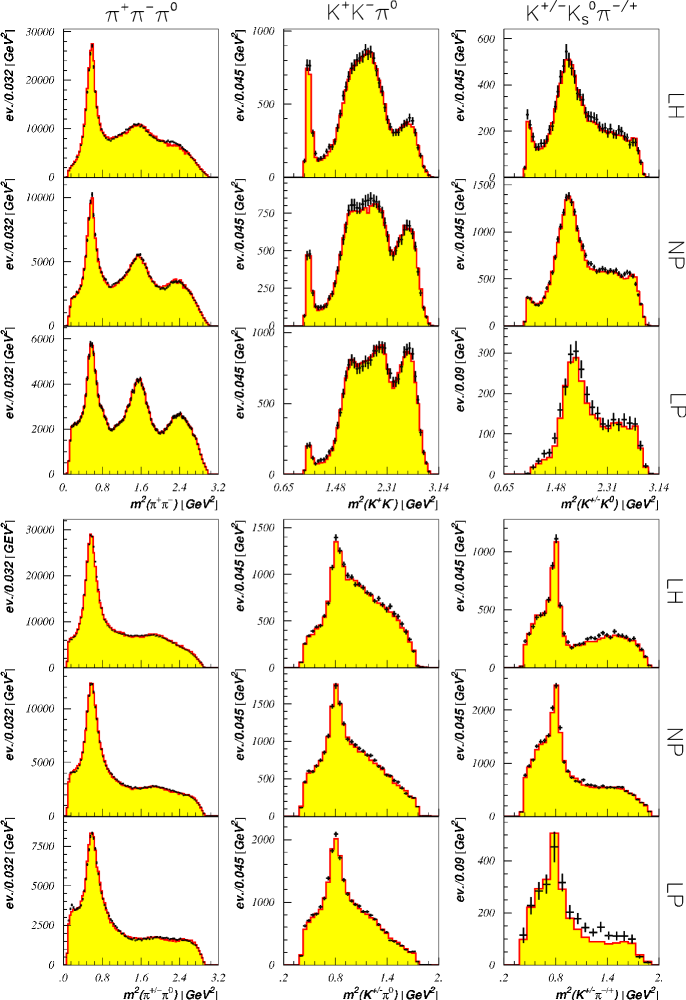
This selection rule is partly confirmed in annihilation from atomic P-states. Recently, the Obelix collaboration reported a pressure-dependent study of $\bar{\mathrm{p}}\mathrm{p}$ annihilation into $\pi^{+}\pi^{-}\pi^{0}$, $\mathrm{K}^{+}\mathrm{K}^{-}\pi^{0}$, and $\mathrm{K}^{\pm}\mathrm{K_{s}}\pi^{\mp}$. Figure 18 shows the $\pi^{+}\pi^{-}$ and $\pi^{\pm}\pi^{0}$ invariant mass distributions for $\bar{\mathrm{p}}\mathrm{p}$ annihilation at rest in liquid H₂, with $\sim(87.5\pm 2.0)\%$ S-state, $\sim(12.5\pm 2.0)\%$ P-state capture and in gaseous H₂ at atmospheric pressure (with $\sim(36\pm 3)\%$ S-state, $\sim(64\pm 3)\%$ P-state capture, and at very low pressure, with $\sim(11\pm 7)\%$ S-state, $\sim(89\pm 7)\%$ P-state capture.

The comparison of the upper two plots showing the $\pi^{+}\pi^{-}$ and $\pi^{\pm}\pi^{0}$ (squared) invariant mass distributions in liquid H₂ confirms the observations of the Crystal Barrel data: the peak height for the $\rho^{0}$ is nearly as large as the peak height of the charged $\rho^{\pm}$: isoscalar initial states must dominate the reaction. Since there is S-state capture dominance, the most important contribution has to come from the ${}^{3}\rm S_{1}$ protonium state. The two lower plots, from annihilation at low pressure, show a more significant $\rho^{\pm}$ signal. The $\rho^{0}$ is reduced by approximately 30%. This would indicate that 2/3 of all annihilations at low pressure are from the isoscalar, and 1/3 from the isovector component of the protonium atom. Inspection of Table 35 shows that the isovector P-states have a statistical weight 8, the isoscalar ones a weight 3. Taking this into account, the $\rho\pi$ puzzle is present also in annihilation with a large P-state capture probability, even though less pronounced. More remarkable is, however, the result of the partial wave analysis that the ${}^{1,1}{{\mathrm{P}}}_{1}$ level decays only weakly into $\rho\pi$ with $\ell=0$:

$$\frac{\rm\mathrm{AF}(\bar{\mathrm{p}}\mathrm{p}\to\rho^{\pm}\pi^{\mp},{}^{1}{{\mathrm{P}}}_{1},{\ell=2})}{\rm\mathrm{AF}(\bar{\mathrm{p}}\mathrm{p}\to\rho^{\pm}\pi^{\mp},{}^{1}{{\mathrm{P}}}_{1},{\ell=0})}=8.1\pm 2.0~{}.$$ (7.2)

This is a surprise: as seen in Table 5, ${}^{1,1}{{\mathrm{P}}}_{1}$ is forbidden to decay into most simple two-meson modes ($\pi\pi$, $\mathrm{K}\overline{\mathrm{K}}{}$, $\pi\omega$, …), and one would naively expect this channel to make full use of the $\rho\pi$ mode, in particular in S-wave ($\ell=0$). The decay ${}^{1,1}{{\mathrm{P}}}_{1}\to\rho\pi$ with $\ell=0$ seems to be dynamically suppressed.

7.2 Annihilation into ${\mathrm{a}}_{2}(1320)$$\pi$

A further dynamical selection rule similar to the $\rho\pi$ puzzle is observed in $\bar{\mathrm{p}}\mathrm{p}$ annihilation into ${\mathrm{a}}_{2}(1320)\pi$. Figure 19

Figure 19: The $\pi^{+}2\pi^{0}$, $\pi^{+}\pi^{-}\pi^{0}$, and $\pi^{-}2\pi^{0}$ invariant mass distributions from $\bar{\mathrm{p}}\mathrm{p}$ annihilation into the $\pi^{+}\pi^{-}2\pi^{0}$ final state. There are two entries per event for the $\pi^{+}\pi^{-}\pi^{0}$ mass plot. All three distributions show a broad peak due to the ${\mathrm{a}}_{2}(1320)\pi$ production. The number of neutral ${\mathrm{a}}_{2}(1320)$ is not visibly smaller than that of charged ${\mathrm{a}}_{2}(1320)$.

shows the most direct evidence for this rule, from Crystal Barrel data on the $\pi^{+}\pi^{-}2\pi^{0}$ final state. In the 3-pion invariant mass distribution, clear evidence for the intermediate ${\mathrm{a}}_{2}(1320)$ decaying into $\rho\pi$ is seen. The strength of the ${\mathrm{a}}_{2}(1320)$ in the three plots is about the same. Now, annihilation into ${\mathrm{a}}_{2}^{\pm}(1320)\pi^{\mp}$ is allowed from both the ${}^{1,1}{{\mathrm{S}}}_{0}$ and the ${}^{3,3}{{\mathrm{S}}}_{1}$ initial state while ${\mathrm{a}}_{2}^{0}(1320)\pi^{0}$ is forbidden from ${}^{3,3}{{\mathrm{S}}}_{1}$. Both processes require $\ell=2$ between ${\mathrm{a}}_{2}(1320)$ and the pion. The fact that the rates for production of charged ${\mathrm{a}}_{2}(1320)$ and neutral ${\mathrm{a}}_{2}(1320)$ mesons are not too different entails that ${\mathrm{a}}_{2}(1320)\pi$ production is preferred from the isoscalar ${}^{1,1}{{\mathrm{S}}}_{0}$ state and suppressed from the isovector ${}^{3,3}{{\mathrm{S}}}_{1}$ initial state. Again, there is no known reason for the suppression of one initial state compared to another initial state. The suppression is due to a dynamical selection rule.

The data shown above were not analysed for the different partial-wave contributions. They are shown here only since they visualise best the new dynamical selection rule. Partial wave analyses were performed on bubble-chamber data, with the ${\mathrm{a}}_{2}(1320)$ decaying into $\rho\pi$, $\eta\pi$, and $\mathrm{K}\overline{\mathrm{K}}{}$. The partial wave analyses confirm the qualitative observation discussed above: annihilation into ${\mathrm{a}}_{2}(1320)$$\pi$ is strong from the $I=0$ initial state (${}^{1}{{\mathrm{S}}}_{0}$) and weak from the $I=1$ component of the ${}^{3}{{\mathrm{S}}}_{1}$ state, with a ratio, see Table 29,

$$\frac{\mathrm{BR}({}^{3,3}{{\mathrm{S}}}_{1}\to{\mathrm{a}_{2}}\pi)}{\,\mathrm{BR}({}^{1,1}{{\mathrm{S}}}_{0}\to{\mathrm{a}_{2}}\pi)}=\frac{6.4\pm 1.2}{82.0\pm 12.0}~{}.$$ (7.3)

The ${\mathrm{a}}_{2}(1320)$$\pi$ annihilation mode from the isovector component of the protonium atom is suppressed by one order of magnitude compared to annihilation from the isoscalar component. This is the same dynamical selection rule as the $\rho\pi$ puzzle.

7.3 Annihilation into $\pi\pi$

There is a related observation in $\bar{\mathrm{p}}\mathrm{p}$ annihilation into $\pi\pi$ and into $\mathrm{K}\overline{\mathrm{K}}{}$. The branching ratios into $\mathrm{K}\overline{\mathrm{K}}{}$ and into $\pi\pi$ depend strongly on the initial state. In Table 36 the relevant branching ratios are listed. Branching ratios determined from $\bar{\mathrm{n}}$p scattering are included in the table.

The ratio of $\mathrm{K}\overline{\mathrm{K}}{}$ versus $\pi\pi$ production is about 1 in annihilation from the ${}^{3}{{\mathrm{S}}}_{1}$ state and less than 0.1 for annihilation from ${}^{3}{{\mathrm{P}}}_{0}$. This result was interpreted as $\mathrm{K}\overline{\mathrm{K}}{}$ suppression in P-wave annihilation [305]. The (corrected) branching ratios in Table 36 show that, instead, $\pi\pi$ production is suppressed in annihilation from the ${}^{3}{{\mathrm{S}}}_{1}$ state and not $\mathrm{K}\overline{\mathrm{K}}{}$ in P-wave annihilation. This interpretation is also favoured by a comparison of cross sections for annihilation in flight. The cross sections for annihilation into $\pi\pi$ and into $\rho\pi$ are very similar in size, while at rest the annihilation frequencies differ by one order of magnitude. Hence we interpret the change in the $\mathrm{K}\overline{\mathrm{K}}{}/\pi\pi$ ratio as suppression of the $\pi\pi$ frequency in the ${}^{3}{{\mathrm{S}}}_{1}$ state.

Table 36: Branching ratios in units of 10^-3 for $\bar{\mathrm{p}}\mathrm{p}$ and $\bar{\mathrm{n}}\mathrm{p}$ annihilation at rest into $\pi\pi$ and into $\mathrm{K}\overline{\mathrm{K}}{}$, from Table 29 and Eqs. (6.14), (6.14). An x indicates that the transition is forbidden.

$\overline{\mathrm{N}}\mathrm{N}$	$\pi\pi$	$\mathrm{K}^{+}\mathrm{K}^{-}$	$\mathrm{K_{s}}\mathrm{K_{l}}$	$\mathrm{K_{s}}\mathrm{K_{s}}+\mathrm{K_{l}}\mathrm{K_{l}}$	$\pi^{+}\pi^{0}$	$\mathrm{K}^{+}\overline{\mathrm{K}}{}^{0}$
${}^{3}{{\mathrm{S}}}_{1}$	$2.79\pm 0.18$	$1.47\pm 0.06$	$1.31\pm 0.07$	x	$4.1\pm 0.7$	$3.5\pm 0.5$
${}^{3}{{\mathrm{P}}}_{0}$	$54.3\pm 1.5$	$4.2\pm 0.3$	x	$0.79\pm 0.15^{*}$

^∗The branching ratio for $\bar{\mathrm{p}}\mathrm{p}\to\mathrm{K_{s}}\mathrm{K_{s}}+\mathrm{K_{l}}\mathrm{K_{l}}$ is reduced by a factor of 2 due to Bose symmetry.

Annihilation into $\pi\pi$ from the ${}^{3}{{\mathrm{S}}}_{1}$ initial state proceeds via the isovector component of the $\bar{\mathrm{p}}\mathrm{p}$ system: again annihilation from the isovector part of the protonium wave function into two isovector particles is suppressed, by about one order of magnitude.

Obviously, there is a common property in these three cases. Annihilation into two isovector mesons such as $\pi\pi$, $\rho\pi$ and ${\mathrm{a}}_{2}(1320)$$\pi$ is strong from isoscalar initial states. In the language of SU(3)_F flavour symmetry, to be described later in this review, the transition from an isoscalar protonium state to two isovector mesons corresponds to a symmetric $D$ coupling that is large. The transition from an isovector protonium state to two isovector mesons, described by an (antisymmetric) $F$ coupling, is weak.

7.4 Annihilation into $\mathrm{K}\overline{\mathrm{K}}{}$

The annihilation frequencies listed in Table 36 reveal another surprising fact: the annihilation frequencies into $\mathrm{K}^{+}\mathrm{K}^{-}$ and $\mathrm{K_{s}}\mathrm{K_{l}}$ differ only by 10%. Assuming an isospin-blind annihilation potential, annihilation into $\mathrm{K}^{+}\mathrm{K}^{-}$ or into $\mathrm{K_{s}}\mathrm{K_{l}}$ (depending on the relative phase of the $I=0$ and $I=1$ amplitudes) could be suppressed in the same way as the charge exchange reaction $\bar{\mathrm{p}}\mathrm{p}\to\bar{\mathrm{n}}\mathrm{n}$ is in a scattering situation. On the other hand, if only one isospin component of the protonium wave function contributes to the process, the two annihilation frequencies must be identical.

Assuming that one isospin component dominates annihilation into a $\rm K\overline{\mathrm{K}}{}$ pair, it can be identified by comparison with the reaction $\bar{\mathrm{n}}\mathrm{p}\to\mathrm{K}^{+}\overline{\mathrm{K}}{}^{0}$. The branching ratio for the latter reaction should be either close to zero (for an isoscalar transition operator), or close to the sum of annihilation frequencies into $\rm K^{+}K^{-}$ and $\mathrm{K_{s}}\mathrm{K_{l}}$ $(2.78\pm 0.09)\times 10^{-3}$ if the transition operator is iso-vectorial. The experimental value $(3.47\pm 0.53)\times 10^{-3}$ requires $I=1$. Why is the annihilation reaction

$$\bar{\mathrm{p}}\mathrm{p}\,({}^{3,3}{{\mathrm{S}}}_{1})\to\mathrm{K}^{+}\mathrm{K}^{-}-\mathrm{K}^{0}\overline{\mathrm{K}}{}^{0}~{},\quad\hbox{strong}~{},$$ (7.4)

and

$$\bar{\mathrm{p}}\mathrm{p}\,({}^{1,3}{{\mathrm{S}}}_{1})\to\mathrm{K}^{+}\mathrm{K}^{-}+\mathrm{K}^{0}\overline{\mathrm{K}}{}^{0}~{},\quad\hbox{weak?}$$ (7.5)

There is no known reason for the suppression of one isospin channel with respect to the other channel. It is a dynamical selection rule.

7.5 Annihilation into $\mathrm{K}^{\pm}\mathrm{K_{s}}\pi^{\mp}$ and $\mathrm{K}^{\pm}\mathrm{K_{l}}\pi^{\mp}$

A similar selection rule is seen in $\bar{\mathrm{p}}\mathrm{p}\to\mathrm{K}^{\pm}\mathrm{K_{s}}\pi^{\mp}$. Figure 20 shows (on the right) the Crystal Barrel data on this reaction. The most striking feature are the two $\mathrm{K}^{*}$ bands ($\mathrm{K}^{\pm}\pi^{\mp}$ and $\mathrm{K_{s}}\pi^{\mp}$). The two bands cross but show little intensity at the crossing on the diagonal, where the two $\mathrm{K}^{*}$ masses are identical. Obviously, the two amplitudes (for $\mathrm{K}^{\star 0}$ and $\mathrm{K}^{\star\pm}$ production) interfere destructively.

Figure 20: The experimental Dalitz plot for the reaction $\bar{\mathrm{p}}\mathrm{p}\to\mathrm{K}^{\pm}\mathrm{K_{s}}\pi^{\mp}$ (liquid H₂). The experimental data (from Crystal Barrel) are shown on the right; on the left are Dalitz plots expected for annihilation from the various possible S-wave components of protonium.

The following discussion is restricted to S-state capture. The final state $\mathrm{K}^{\pm}\mathrm{K_{s}}\pi^{\mp}$ does not have defined $G$-parity, and both isospin components may contribute to the annihilation process. There are four initial states which may contribute to the Dalitz plot in Fig. 20 (right). On the left, Fig. 20 shows the Dalitz plots expected for the four allowed initial states. The ${}^{1}{{\mathrm{S}}}_{0}$ initial state is characterised by a $\cos^{2}\Theta$ angular distribution, with high intensity at the ends with $\cos\Theta=\pm 1$. The ${}^{3}{{\mathrm{S}}}_{1}$ state produces a $\sin^{2}\Theta$ distribution and the intensity vanishes at the ends. The Dalitz plot expected for the isovector and the isoscalar component of the protonium wave function differ by their interference pattern.

It is obvious from the comparison of data and theoretical Dalitz plots that the two theoretical Dalitz plots with destructive interference between the two $\mathrm{K}^{*}\mathrm{K}$ amplitudes are the ones contributing most to the final state. This observation is confirmed in partial wave analyses, see Table 22, where the contributions to $\mathrm{K}^{*}\mathrm{K}$ production are listed. The sum of the two partial waves with destructive interference exceeds the sum of constructive interference by one order of magnitude.

This dynamical selection rule can be interpreted at the level of the produced $\mathrm{K}^{*}$. For this purpose the decomposition of the $\mathrm{K}^{*}$ contribution into the final-state particles needs to be considered:

 

$${{}\left|{}^{3,3}{{\mathrm{S}}}_{1}\right>\to\left|I^{C}=1^{-}\right>=\textstyle\frac{1}{2}\left(\left|\mathrm{K}^{*+}\mathrm{K}^{-}\right>-\left|\mathrm{K}^{*0}\overline{\mathrm{K}}{}{}^{0}\right>+\left|\mathrm{K}^{*-}\mathrm{K}^{+}\right>-\left|\overline{\mathrm{K}}{}{}^{*0}\mathrm{K}^{0}\right>\right)\quad\rm strong~{},}$$

  (7.6)

In the Dalitz plots, Fig. 20, interference between the $\mathrm{K}^{*\pm}$ and $\overline{\mathrm{K}}{}{}^{*0}$ is observed. Interference occurs in a given final state; the $\mathrm{K}^{*}$ has to be expanded into its decay products to appreciate the meaning of the interference pattern. The next two lines give the final states produced in the above reactions.

$$\hbox{}\,\vbox{\openup 3.0pt\halign{\strut\hfil$\displaystyle{#}$&$\displaystyle{{}#}$\hfil&&\strut\hfil$\displaystyle{#}$&$\displaystyle{{}#}$\hfil\cr&\phantom{-}\left|(\pi^{0}\mathrm{K}^{+})\mathrm{K}^{-}\right>\qquad\left|(\pi^{-}\mathrm{K}^{+})\mathrm{K_{s}}\right>\qquad&&\left|(\pi^{0}\mathrm{K}^{-})\mathrm{K}^{+}\right>\qquad\underline{\left|(\pi^{+}\mathrm{K}^{-})\mathrm{K_{s}}\right>}\cr&\underline{-\left|(\pi^{+}\mathrm{K_{s}})\mathrm{K}^{-}\right>}\qquad\left|(\pi^{0}\,\mathrm{K_{s}})\,\mathrm{K_{s}}\right>\qquad-&&\left|(\pi^{-}\mathrm{K_{s}})\mathrm{K}^{+}\right>\qquad\left|(\pi^{0}\,\mathrm{K_{s}})\,\mathrm{K_{s}}\right>\crcr}}\,~{}.$$ (7.7)

A pair of final states in which the $\mathrm{K}^{*}$ can interfere is underlined in (7.7). These two states have $\mathrm{K}^{*+}\mathrm{K}^{-}$ and $\overline{\mathrm{K}}{}{}^{*0}\mathrm{K}^{0}$ intermediate states, the first and the last entries in Eq. (7.6). The two annihilation modes marked strong in (7.6) produce the $\mathrm{K}^{*}\mathrm{K}$ in the form $\mathrm{K}^{*+}\mathrm{K}^{-}-\overline{\mathrm{K}}{}{}^{*0}\mathrm{K}^{0}$ and the two weak modes in the form $\mathrm{K}^{*+}\mathrm{K}^{-}+\overline{\mathrm{K}}{}{}^{*0}\mathrm{K}^{0}$. It is not the isospin which drives this dynamical selection rule: the two initial states contributing strongly are

 

$${{}{}^{3,3}{{\mathrm{S}}}_{1}\ \to\ \mathrm{K}^{*+}\mathrm{K}^{-}-\mathrm{K}^{*0}\overline{\mathrm{K}}{}{}^{0}+\hbox{c.c.}\quad\hbox{strong}~{},}$$

  (7.8)

while the two states

 

$${{}{}^{1,3}{{\mathrm{S}}}_{1}\ \to\ \mathrm{K}^{*+}\mathrm{K}^{-}+\mathrm{K}^{*0}\overline{\mathrm{K}}{}{}^{0}+\hbox{c.c.}\quad\hbox{weak}~{},}$$

  (7.9)

contribute at most weakly. The charged and neutral $\mathrm{K}^{*}\,\mathrm{K}$ combinations are produced strongly with a relative minus sign.

Inspecting Table 29 shows that $\mathrm{K}^{*}_{2}(1430)$K production exhibits a similar selection rule:

 

$${{}^{3,3}{{\mathrm{S}}}_{1}\ \to\ \mathrm{K}_{2}^{*+}\mathrm{K}^{-}-\mathrm{K}_{2}^{*0}\overline{\mathrm{K}}{}^{0}+{\rm c.c.}}$$

  (7.10)

The dominance of one isospin channel for these decay modes may be surprising since the nominal mass of the $\mathrm{K}_{2}^{*}(1430)$ plus the mass of the $\mathrm{K}$ exceed the available energy. Hence rescattering of the final-state particles is expected to play a large role.

Equations (7.6) suggest a pattern of strongly and weakly produced $\mathrm{K}$ and $\mathrm{K}{}^{*}$ which depends on charge conjugation and isospin of the initial state. This generalisation can be tested in annihilation from atomic P-states. The Obelix collaboration has measured the density dependence of $\mathrm{K}\overline{\mathrm{K}}{}\pi$ production, see Fig. 18. Also here, a preference for one isospin for $\mathrm{K}\mathrm{K}{}^{*}$ production is observed; the prevailing isospin channel is shown in Table 30. For the ${}^{3}{{\mathrm{P}}}_{1}$ initial state, the expectation is fulfilled, for the ${}^{1}{{\mathrm{P}}}_{1}$ and ${}^{3}{{\mathrm{P}}}_{2}$ not. Annihilation from P-states seems not to follow the same simple pattern as observed in S-state annihilation.

In the $\mathrm{K}^{+}\mathrm{K}^{-}\pi^{0}$ final state, a clear signal due to $\phi$ production is seen. The final state $\phi\pi$ can be produced only from states with negative charge conjugation and with isospin $I=1$. Thus only the ${}^{3,3}{{\mathrm{S}}}_{1}$ and ${}^{3,1}{{\mathrm{P}}}_{1}$ states can contribute. At high density, the $\phi$ is strong, but weak at low densities, indicating a preference for the ${}^{3,3}{{\mathrm{S}}}_{1}$ initial state. If $\phi$’s are produced as two-step process, through $\mathrm{K}^{*}\overline{\mathrm{K}}{}$ and rescattering of the two kaons into a $\phi$, then $\mathrm{K}^{*}\overline{\mathrm{K}}{}$ should be strong in ${}^{3,3}{{\mathrm{S}}}_{1}$ (which is the case) and weak in ${}^{3,1}{{\mathrm{P}}}_{1}$. This finding is supported by the partial wave analysis of the data of Fig. 18 where the ${}^{3,1}{{\mathrm{P}}}_{1}$ couples weaker to $\mathrm{K}^{*}\overline{\mathrm{K}}{}$ than ${}^{1,1}{{\mathrm{P}}}_{1}$. This question will be addressed again in Sec. 8.7.

7.6 Annihilation into $\mathrm{K}^{*}\overline{\mathrm{K}}{}{}^{*}$

The frequency for $\bar{\mathrm{p}}\mathrm{p}$ annihilation into $\mathrm{K}^{*}\overline{\mathrm{K}}{}^{*}$ was determined in the BNL bubble chamber experiment [47]:

 

$${\mathrm{AF}(\bar{\mathrm{p}}\mathrm{p}\to\mathrm{K}^{*+}\mathrm{K}^{*-})}$$

  (7.11)

The more recent annihilation frequencies from Crystal Barrel are at variance with these findings.

The Crystal Barrel collaboration has studied the dynamics of annihilation into two $\mathrm{K}^{*}$, in the final states $\mathrm{K_{s}}\mathrm{K_{l}}\pi^{0}\pi^{0}$ [191] and $\mathrm{K}^{\pm}\mathrm{K_{s}}\pi^{\mp}\pi^{0}$ [192]. The former is forced to proceed via the ${}^{3}{{\mathrm{S}}}_{1}$ initial state, and is dominated by $\mathrm{K}^{*}\overline{\mathrm{K}}{}{}^{*}$ production. The two $\mathrm{K}^{*}$ are produced with $\ell=1$ between them; the two $\mathrm{K}^{*}$ spins add up to $S=0$ or $2$ with about equal amplitudes and opposite phases; the contribution from $S=1$ is small. The absolute annihilation frequencies were not determined.

In the reaction $\mathrm{K}^{\pm}\mathrm{K_{s}}\pi^{\mp}\pi^{0}$, $\mathrm{K}^{*}\overline{\mathrm{K}}{}^{*}$ production plays a less significant role. The fractional contributions in the partial wave analysis can be normalised to the annihilation frequency of the reaction channel (given in Table 9) to arrive at the following branching ratios:

 

$${\mathrm{BR}(\bar{\mathrm{p}}\mathrm{p}({}^{3}{{\mathrm{S}}}_{1})\to\mathrm{K}^{*+}\mathrm{K}^{*-})}$$

  (7.12)

Annihilation from the ${}^{3}{{\mathrm{S}}}_{1}$ state requires $\ell=1$; spin states $S=0$ and $S=2$ both contribute. As above, the amplitudes are similar in magnitude but opposite in phase. However, the dominance of $\mathrm{K}^{*+}\mathrm{K}^{*-}$ over $\mathrm{K}^{*\,0\,}\overline{\mathrm{K}}{}^{*\,0\,}$ shows that both isospin channels contribute.

Annihilation from the ${}^{1}{{\mathrm{S}}}_{0}$ initial state may proceed with $\ell=0$ and with one total spin only, $S=1$. The frequency for $\mathrm{K}^{*}\overline{\mathrm{K}}{}^{*}$ production is larger, and the two charge modes are about equal in size. The measured phase between the two amplitudes is $-50^{\circ}$. Hence we do not find the dynamical selection rules as in the other annihilation modes into strange final-state mesons.

We note that in $\bar{\mathrm{p}}\mathrm{p}\to\mathrm{K}^{*}\mathrm{K}^{*}$, the $\mathrm{K}^{*}$ momenta are $285\,{\mathrm{Me\hskip-1.0ptV}\hskip-2.0pt/\hskip-1.0ptc}$ and the two $\mathrm{K}^{*}$ decay before having left the strong interaction volume. $\mathrm{K}^{*}\overline{\mathrm{K}}{}^{*}$ production constitutes only a small fraction of the final state and rescattering of the final-state particles presumably has a decisive influence. Hence it is not surprising that this reaction does not exhibit any striking dynamical selection rule.

7.7 Discussion of the dynamical selection rules

Table 37 summarises the most important selection rules. Weak and strong are meant as relative weights; annihilation into ${\mathrm{a}}_{2}(1320)$$\pi$ from $I=1$ is listed as weak even though it is a larger branching ratio than the one for $\mathrm{K}\overline{\mathrm{K}}{}$ annihilation. But for a given final state, a strong decay mode has a branching ratio exceeding its associate weak decay mode by about one order of magnitude.

Table 37: Summary of the most important dynamical selection rules. A cross x indicates $G$-parity forbidden reactions.

${}^{2S+1}L_{J}\,(\bar{\mathrm{p}}\mathrm{p})$	$I=0$	$I=1$	${}^{2S+1}L_{J}\,(\bar{\mathrm{p}}\mathrm{p})$	$I=0$	$I=1$
${}^{3}{{\mathrm{S}}}_{1}$$\to\rho\pi$	strong	x	${}^{3}{{\mathrm{S}}}_{1}$$\to\mathrm{K}\overline{\mathrm{K}}{}$	weak	strong
${}^{1}{{\mathrm{S}}}_{0}$$\to\rho\pi$	x	weak
${}^{1}{{\mathrm{S}}}_{0}$$\to{\mathrm{a}}_{2}(1320)\pi$	strong	x	${}^{3}{{\mathrm{S}}}_{1}$$\to\mathrm{K}^{*}\overline{\mathrm{K}}{}+\mathrm{c.c.}$	weak	strong
${}^{3}{{\mathrm{S}}}_{1}$$\to{\mathrm{a}}_{2}(1320)\pi$	x	weak	${}^{1}{{\mathrm{S}}}_{0}$$\to\mathrm{K}^{*}\overline{\mathrm{K}}{}+\mathrm{c.c.}$	strong	weak
${}^{3}{{\mathrm{P}}}_{0}$$\to\pi\pi$	strong	x	${}^{3}{{\mathrm{S}}}_{1}$$\to\mathrm{K}^{*}_{2}(1430)\overline{\mathrm{K}}{}+\mathrm{c.c.}$	weak	strong
${}^{3}{{\mathrm{S}}}_{1}$$\to\pi\pi$	x	weak	${}^{1}{{\mathrm{S}}}_{0}$$\to\mathrm{K}^{*}_{2}(1430)\overline{\mathrm{K}}{}+\mathrm{c.c.}$	strong	weak

In any reasonable model, the transition rate for annihilation of the $\bar{\mathrm{p}}\mathrm{p}$ system to a two-meson final state is proportional to

1. the probability to find the needed isospin component in the protonium wave function (initial state interaction),

2. the strength of the hadronic transition operator,

3. the probability that the final state is formed.

Are the dynamical selection rules an effect of initial state interaction? Annihilation of the ${}^{1,3}{{\mathrm{S}}}_{1}$ level to $\rho\pi$ is strong, hence the isoscalar component of the protonium ${}^{3}{{\mathrm{S}}}_{1}$ wave function must be enhanced. Annihilation from ${}^{3,3}{{\mathrm{S}}}_{1}\to\pi\pi$ is weak, hence the isotriplet component of the wave function must be small at this momentum. From ${}^{1,3}{{\mathrm{S}}}_{1}$ and ${}^{3,3}{{\mathrm{S}}}_{1}$ annihilation into open strangeness we conclude that the ${}^{3}{{\mathrm{S}}}_{1}$ isoscalar component must be small. A component can hardly be enhanced and suppressed at the same time. If the initial state interaction is responsible, there must be a strong momentum dependence of this suppression and enhancement. Note, however, that the protonium wave function, as calculated in potential models, sometimes exhibit oscillations, see, e.g., [306].

Table 38 lists the dominant isospin component of protonium wave functions, the momentum at which it should prevail, and the final state from which the conclusion is drawn. In particular for the ${}^{3}{{\mathrm{S}}}_{1}$ state, an oscillating wave function would result. Translated into a spatial wave function, the isoscalar part should dominate at 0.21; 0.26; and 0.43 fm, the isovector one at 0.25 and 0.32 fm. Extremely sharp oscillations between isovector and isoscalar components would be needed.

Table 38: Interpretation of the dynamical selection rules as an effect of the initial state interaction. The Table gives the prevailing isospin component of protonium at a given momentum if the origin of the dynamical selection rules is assigned to the initial state interaction. The reaction from which the dominant isospin component is determined is given in the last column.

${}^{2S+1}L_{J}\,(\bar{\mathrm{p}}\mathrm{p})$	dominant isospin	${}^{2S+1}L_{J}\,(\bar{\mathrm{p}}\mathrm{p})$	dominant isospin	at momentum	From
${}^{3}{{\mathrm{S}}}_{1}$	$I=0$	${}^{3}{{\mathrm{P}}}_{0}$	$I=0$	928 $\,{\mathrm{Me\hskip-1.0ptV}\hskip-2.0pt/\hskip-1.0ptc}$	$\pi\pi$
${}^{3}{{\mathrm{S}}}_{1}$	$I=1$	${}^{1}{{\mathrm{S}}}_{0}$	$I=1$	797 $\,{\mathrm{Me\hskip-1.0ptV}\hskip-2.0pt/\hskip-1.0ptc}$	$\mathrm{K}\overline{\mathrm{K}}{}+\mathrm{c.c.}$
${}^{3}{{\mathrm{S}}}_{1}$	$I=0$	${}^{1}{{\mathrm{S}}}_{0}$	$I=0$	773 $\,{\mathrm{Me\hskip-1.0ptV}\hskip-2.0pt/\hskip-1.0ptc}$	$\rho\pi$
${}^{3}{{\mathrm{S}}}_{1}$	$I=1$	${}^{1}{{\mathrm{S}}}_{0}$	$I=0$	616 $\,{\mathrm{Me\hskip-1.0ptV}\hskip-2.0pt/\hskip-1.0ptc}$	$\mathrm{K}^{*}\overline{\mathrm{K}}{}+\mathrm{c.c.}$
${}^{3}{{\mathrm{S}}}_{1}$	$I=0$	${}^{1}{{\mathrm{S}}}_{0}$	$I=0$	460 $\,{\mathrm{Me\hskip-1.0ptV}\hskip-2.0pt/\hskip-1.0ptc}$	${\mathrm{a}}_{2}(1320)\pi$
${}^{3}{{\mathrm{S}}}_{1}$	$I=1$	${}^{1}{{\mathrm{S}}}_{0}$	$I=0$	$\sim 120$ $\,{\mathrm{Me\hskip-1.0ptV}\hskip-2.0pt/\hskip-1.0ptc}$	$\mathrm{K}^{*}_{2}\overline{\mathrm{K}}{}+\mathrm{c.c.}$

However, tensor forces induce ${}^{1,3}{{\mathrm{D}}}_{1}$ and ${}^{3,3}{{\mathrm{D}}}_{1}$ components in the protonium wave function, which contribute to annihilation. Maruyama et al. [307], for instance found that in the framework of a specific model with planar diagrams, “inclusion of D states solve the $\rho\pi$ puzzle.”

The role of final-state interaction in the $\rho\pi$ puzzle was underlined by Mull et al. [308]. For the ${}^{3,1}{{\mathrm{S}}}_{0}:{}^{1,3}{{\mathrm{S}}}_{1}$ ratio they found about 1:5 without final-state interaction and 1:25 when it is added. Surprisingly, the effect is not due to the $\rho\pi$ interaction of their model being different in these two states, but simply to the existence of this interaction. The effect is almost negligible for P-wave annihilating into $\rho\pi$.

Anyhow, the interaction between final state mesons is not well known, and thus one must rely on models. In the case of a well pronounced resonance, one could expect all channels, e.g., $\pi\pi$, $\mathrm{K}\overline{\mathrm{K}}{}$, etc, to feel attractive forces. In other circumstances, channels that are weakly coupled might behave differently. We conclude that final state interaction cannot be neglected, but is not demonstrated to explain all observed dynamical selection rules.

Alternatively, we may try to understand the dynamical selection rules as the effect of an hadronic transition operator. Then we find that the transition to two isovector mesons is small from the isovector component of protonium wave functions (at least for ${}^{3}{{\mathrm{S}}}_{1}$ and ${}^{1}{{\mathrm{S}}}_{0}$) and large for the isosinglet component. The remaining dynamical selection rules are condensed into the observation that in $\bar{\mathrm{p}}\mathrm{p}$ annihilation, kaons (and $\mathrm{K}^{*}$, ..) are produced in the form $\mathrm{K}^{+}\mathrm{K}^{-}$ and in $\mathrm{K}^{0}\overline{\mathrm{K}}{}{}^{0}$. Whenever we probe the annihilation potential with two isovector mesons in the final state, we find a large isospin $I=0$ contribution. When we probe the annihilation potential with final states with open strangeness, we find the combination $\bar{\mathrm{p}}\mathrm{p}\to\mathrm{K}^{+}\mathrm{K}^{-}-\mathrm{K}^{0}\overline{\mathrm{K}}{}{}^{0}$ to be large compared to $\bar{\mathrm{p}}\mathrm{p}\to\mathrm{K}^{+}\mathrm{K}^{-}+\mathrm{K}^{0}\overline{\mathrm{K}}{}{}^{0}$.

We conclude that the dynamical selection rules can economically be interpreted as suppression of specific hadronic transition operators. The hadronic operator acts in a similar way for two pseudoscalar mesons, for a pseudoscalar and a vector and for a pseudoscalar and a tensor meson. The dynamical selection rules drive annihilation preferentially into specific favoured flavour combinations; other quantum numbers like spin and angular momentum of the final-state mesons are seemingly less relevant.

It is not easy to find a microscopic derivation of such a selection rule. An attempt was made by Niskanen and Myhrer [309], who analysed quark–antiquark annihilation (necessary for $\overline{\mathrm{N}}\mathrm{N}\to\rho\pi$) into one or two gluons and found, interestingly, that it is suppressed if the $\overline{\mathrm{N}}\mathrm{N}$ initial state is ${}^{3,1}{{\mathrm{S}}}_{0}$. A non-perturbative generalisation would be desirable.

8 Phenomenological analysis

There is an abundant literature on $\overline{\mathrm{N}}\mathrm{N}$ annihilation. This complex process has been studied in a variety of models. Most detailed numerical analyses are now obsolete, to the extent that the parameters of the models have been tuned to reproduce early and incomplete sets of data. However, the underlying mechanisms still deserve to be presented and compared to other possible mechanisms.

In this section, we will expand on the following questions: the pion multiplicity and the clustering of mesons into resonances; the range of annihilation; the role of initial and final state interaction; the importance of symmetries; the probability of producing strange mesons and the mechanisms of OZI violation; the interpretation of dynamical selection rules. Ideally, answers to these questions should come from a full understanding of hadronic interactions which we do not yet have.

8.1 Initial state interaction

8.1.1 Overall suppression

Before considering annihilation mechanisms, it is important to underline the role of initial-state interactions. If a specific process $\overline{\mathrm{N}}\mathrm{N}\to m_{1}m_{2}\ldots$ is calculated in a given model without accounting for initial-state interactions, its rate is overestimated by orders of magnitude. In more technical words, a Born-approximation treatment is unacceptable, while a distorted-wave Born approximation can be rather realistic. In any realistic model, the $\overline{\mathrm{N}}\mathrm{N}$ wave function is dramatically suppressed at short distances by the cumulative effect of annihilation channels.

8.1.2 Induced channels

A serious warning by Green et al. (see, e.g., [310]), is that if initial-state interactions are taken seriously with our current ideas on nuclear forces, there are ample transition amplitudes $\overline{\mathrm{N}}\mathrm{N}\leftrightarrow\mathrm{N}^{*}\overline{\mathrm{N}}+\mathrm{c.c.}$, or $\overline{\mathrm{N}}\mathrm{N}\leftrightarrow\mathrm{N}^{*}\overline{\mathrm{N}}{}^{*}$, with at least one baryon or antibaryon being a spin ($\mathrm{N}^{*}=\Delta$), orbital or radial excitation of the nucleon. Similarly strange-meson production can proceed via a $\overline{\Lambda}\Lambda$ doorway or other hyperon–antihyperon intermediate states. Hence the quark content of the initial state does not reduce to $(uud\bar{u}\bar{u}\bar{d})$. This might influence the conclusions drawn about the hierarchy of various quark diagrams describing annihilation.

8.1.3 Selective suppression

Even for ratios of branching ratios, a pure Born–Oppenheimer treatment of annihilation might be misleading, as different initial states do not necessarily experience the same suppression, and in a given partial wave, the damping of the wave function depends on the momentum range which is explored (see, e.g., Ref. [306], and discussions later in this section).

The $\overline{\mathrm{N}}\mathrm{N}$ interaction is investigated in scattering and protonium experiments, and described in a number of models that combine long-range meson exchanges and short-range absorption. This subject is discussed in a previous review article [1].

As already stressed in Sec. 4.4.5, the long-range potential has a strong spin and isospin dependence, starting with the one-pion-exchange term which includes a ${\vec{\tau}}_{1}.{\vec{\tau}}_{2}\,{\vec{\sigma}}_{1}.{\vec{\sigma}}_{2}$ operator for the central interaction, and something analogous for the tensor one. In potential models, a dramatic spin–isospin dependence is induced in the various partial waves contributing to annihilation at low energy.

8.1.4 Orbital mixing

Meson-exchange models also predict some“orbital” mixing in natural-parity states of protonium, due to the tensor component of the $\overline{\mathrm{N}}\mathrm{N}$ interaction. For instance, the authors of Ref. [311] combine the so-called “A2” model (to be defined later) with initial-state protonium wave functions estimated from potential models, and computed the relative rates for annihilation into two mesons. Some ratios are found to be extremely sensitive to details of the $\overline{\mathrm{N}}\mathrm{N}$ interaction used to produce the protonium wave-function. In particular, neglecting the ${}^{3}{{\mathrm{D}}}_{1}$ admixture into the ${}^{3}{{\mathrm{S}}}_{1}$ wave function sometimes changes the results by an order of magnitude. It was already noted by Green et al. [312, 310] that the ${}^{3}{{\mathrm{P}}}_{0}$ model requires an orbital momentum between the annihilating quark and antiquark. For an overall S-wave, this is provided by departures from the harmonic-oscillator behaviour of the wave function. For a spin $S=1$ system, an overall $J=1$ state comes either from an S-wave, or, in presence of tensor forces, from a D-wave.

8.1.5 Isospin mixing of protonium

In potential models, the effect of initial-state interaction is predicted to be particularly important in protonium wave functions, as compared to scattering wave functions relevant for annihilation in flight. This was underlined by Kaufmann and Pilkuhn [257], and several other authors.

In short, a pure $\bar{\mathrm{p}}\mathrm{p}$ state corresponds to equal weights for isospin $I=0$ and $I=1$. However, the charge-exchange potential induces transitions from $\bar{\mathrm{p}}\mathrm{p}$ to $\bar{\mathrm{n}}\mathrm{n}$, and when the $\bar{\mathrm{p}}\mathrm{p}$ and $\bar{\mathrm{n}}\mathrm{n}$ amplitudes are recombined into amplitudes of given isospin $I$, one component is often much larger than the other one. For instance, ${}^{3}{{\mathrm{P}}}_{0}$ is clearly dominated by its $I=0$ part. However, this firm prediction of meson-exchange models is not confirmed by studying the systematics of branching ratios. See, for instance, the discussion in Refs. [313, 306, 167]. It is somewhat of a paradox that the pion-exchange force nicely reproduces the pattern of fine splitting of P-levels of protonium [1] as well as the hierarchy of hadronic widths (see Table 11), but resists experimental checks for branching ratios.

The explicit calculation of Ref. [311] illustrates the concerns about isospin mixing in protonium. For instance, the $\eta\rho^{0}$ ($I=1$) to $\pi^{0}\rho^{0}$ ($I=0$) is calculated to be much smaller than the experimental value.

In Ref. [314], Gutsche et al. also discuss this question of isospin mixing. They estimate the rate for radiative annihilation $\bar{\mathrm{p}}\mathrm{p}\to\gamma+X$, with $X$ being $\pi^{0}$, $\eta$, $\eta^{\prime}$, $\rho$ or $\omega$. The transition is sensitive to interference between the $I=0$ and $I=1$ components of the protonium wave function, and thus probes the isospin mixing predicted by potential models. A rather good agreement is found with the data. However, the rate for $\gamma\phi$ cannot be reproduced.

8.1.6 Checking isospin mixing in protonium

The first attempt to deduce the isospin ratios from experiment was made in [313]. The model assumed that the transition matrix element for annihilation into two mesons is entirely determined by the isospins involved. There are transitions from the $I=0$ initial state to two isoscalars and to two isovectors, and from the $I=1$ initial state to one isoscalar and an isovector. The transition matrix elements are then supposed to be independent of the quantum numbers of the initial state, apart from a normalisation which could be different for different initial states. The results are certainly model-dependent, and the errors are large. The isospin-mixing coefficients are found compatible with the predictions of potential models, but, due to the large errors, also with the absence of mixing effects. The subject was further discussed by Dover et al. [306] and more recently by the Crystal Barrel collaboration [209].

Table 39: Ratio of isovector to isoscalar fraction of the protonium wave function for various initial states ^2s+1L_J. The three theoretical values correspond to different $\overline{\mathrm{N}}\mathrm{N}$ potentials, as compiled in Ref. [315].

Initial	Potentials			Data analysis
state	KW	DR1	DR2	Ref.[313]	Ref.[209]
${}^{1}{{\mathrm{S}}}_{0}$	0.68	0.68	0.8	$0.72\,{}^{+0.24}_{-0.18}$	$0.50\,{}^{+0.48}_{-0.29}$
${}^{3}{{\mathrm{S}}}_{1}$	1.22	0.95	1.26	$1.17\,{}^{+0.39}_{-0.28}$	$1.17\,{}^{+0.30}_{-0.23}$
${}^{3}{{\mathrm{P}}}_{0}$	0.03	0.03	0.05	$1.16\pm 0.34$	$0.41\,{}^{+0.11}_{-0.09}$
${}^{3}{{\mathrm{P}}}_{1}$	9.4	9.7	6.5	$9\pm 5$
${}^{1}{{\mathrm{P}}}_{1}$	0.96	0.82	0.61	$0.81\pm 0.51$

8.1.7 Isospin content of $\bar{\mathrm{p}}\mathrm{p}$ in $\bar{\mathrm{p}}\mathrm{d}$

The analysis can be extended to annihilation on deuterium. To our knowledge, there are no published calculation of the detailed isospin content of $\bar{\mathrm{p}}\mathrm{p}$ within $\bar{\mathrm{p}}\mathrm{d}$. Note that the isospin content of the neutral $\bar{\mathrm{p}}\mathrm{p}$ state in $\bar{\mathrm{p}}\mathrm{d}$ is not necessarily the same as in protonium, due to the presence of the third hadron.

The transition $\bar{\mathrm{p}}\mathrm{d}$ into a isovector meson $m_{1}$ and a isoscalar meson $m_{2}$ proceeds via the (squared) isovector component of the $\rm\bar{\mathrm{p}}N$ subsystem. This component is 1 for $\rm\bar{\mathrm{p}}n$ and smaller for $\rm\bar{\mathrm{p}}p$. Thus

 

$${\frac{\mathrm{AF}(\bar{\mathrm{p}}\mathrm{d}\to\pi^{0}\omega+\mathrm{n})}{\mathrm{AF}(\bar{\mathrm{p}}\mathrm{d}\to\pi^{-}\omega+\mathrm{p})}}$$

  (8.1)

The frequencies were obtained by calculating mean values from the numbers given in Table 32. Those normalised to the number of $\bar{\mathrm{p}}\mathrm{d}$ annihilations have been multiplied by 2. The mean values do not include the results from [108]. The $\pi^{-}\omega$ data from [68] and [78] are superseded by a reanalysis [276].

The reaction $\bar{\mathrm{p}}\mathrm{p}$$\to\pi\omega$ is dominated by the ${}^{3}{{\mathrm{S}}}_{1}$ initial state; the ratios (8.1) suggest a mild deviation from a pure $\bar{\mathrm{p}}\mathrm{p}$ system at annihilation for which ratios $0.5$ would be expected. According to Table 41, annihilation into $\pi\eta$ goes through the ${}^{3}{{\mathrm{P}}}_{0}$ isovector component of the $\bar{\mathrm{p}}\mathrm{p}$ system which is calculated to be very small, see Table 39.

8.2 Final state interaction

When discussing annihilation, one can hardly forget the strong interaction of the produced mesons, which are likely to rescatter, form resonances, decay into pions, etc. Even lighter mesons, which escape faster from the interaction region, might be affected.

Final-state interactions were introduced, e.g., by the Bonn group [308] and found to play an important role for the spin effects associated with $\overline{\mathrm{N}}\mathrm{N}\to\pi\pi$ or $\mathrm{\overline{K}K}$, and for the $\rho\pi$ puzzle. We shall see later in this section that it is suggested that rescattering could explain the observed deviations from the OZI rule.

Clearly, if a channel is not or only weakly populated by the main mechanism of annihilation, it might receive a non-negligible contribution of rescattering from another final state. In a fictitious world where $\bar{\mathrm{p}}\mathrm{p}$ does not couple to $\mathrm{K}\overline{\mathrm{K}}{}$, the $\pi\pi\to\mathrm{K}\overline{\mathrm{K}}{}$ reaction would be crucial.

On the other hand, rescattering among channels which are copiously produced, presumably has little effect on the annihilation frequencies. The loss towards other channels is compensated for by the feed-back. More generally, in a regime of strong production, saturation occurs. If one adds another mechanism, the production rate grows less than would naively be expected by adding the squared amplitudes estimated independently.

Consider for instance the following annihilation frequencies for $\omega$ and $\rho$ production:

$$\frac{\mathrm{AF}(\bar{\mathrm{p}}\mathrm{p}\to\pi^{0}\omega)}{\mathrm{AF}(\bar{\mathrm{p}}\mathrm{p}\to\rho^{0}\pi^{0})}=0.41\pm 0.06~{},\qquad\frac{\mathrm{AF}(\bar{\mathrm{p}}\mathrm{p}\to\rho\eta)}{\mathrm{AF}(\bar{\mathrm{p}}\mathrm{p}\to\eta\omega)}=0.23\pm 0.06~{}.$$ (8.2)

There is no obvious dominance of $\rho$ production over $\omega$ production, though the $\rho$ meson is more likely than $\omega$ to be formed in the rescattering of primary mesons.

In short, the final-state interaction is not expected to dominate the systematics of branching ratios, but should be kept in mind for channels which are suppressed.

8.3 Pion multiplicity and two-meson doorway scenario

An average of five pions are produced in nucleon–antinucleon at rest. In a baryon-exchange picture, or in microscopic quark models, it is natural to assume that a few meson resonances are primarily produced, the observed final states resulting from the decay of these resonances. A large, but quantitatively still unknown, fraction of all annihilation modes proceeds even via two-meson intermediate states, sometimes called quasi two-body annihilation. Insisting on two-body annihilation as the dominant contribution however does not account for the large fraction of events leading to high pion multiplicities.

8.3.1 The Vandermeulen model

Vandermeulen [316] suggested that these high pion multiplicities could come from an enhanced production of mesons with high mass. He observed that meson resonances are preferentially produced with nearly the maximal mass which is allowed by phase space. The effect can be parametrised by assuming that annihilation proceeds via two primary mesons and writing the frequency $\bar{\mathrm{p}}\mathrm{p}\to m_{1}+m_{2}$ for producing two mesons with masses $m_{1}$ and $m_{2}$ as proportional to

$$F(q)=q\,\exp\left[-R_{\mathrm{so}}\sqrt{s-(m_{1}+m_{2})^{2}}\right]~{},$$ (8.3)

where $q$ is the momentum of the mesons, as given by Eq. (4.2); $s$ is the Mandelstam variable which is $s=4m_{\mathrm{p}}^{2}$ for annihilation at rest. With a reasonable adjustment at $R_{\mathrm{so}}=1.2\;\mathrm{GeV}^{-1}$, Vandermeulen was able to account for many key features of annihilation in flight, covering a wide range of antiproton momenta. The Crystal Barrel collaboration applied (8.3) to annihilation at rest and derived [167] $R_{\mathrm{so}}=0.83$ GeV^-1. The model of Vandermeulen was further developed, e.g., by Mundigl et al. [317].

To get more insight into Eq. (8.3), we define the annihilation amplitude by $F(q)=q\,|f(q)|^{2}$. For the case of two mesons having the same mass, $f(q)$, thanks to Eq. (4.3), reduces to an exponential function,

$$f(q)=\exp\left[-\frac{R_{\mathrm{so}}}{2}\sqrt{s-(2m_{1})^{2}}\right]=\exp[-qR_{\mathrm{so}}]~{}.$$ (8.4)

This momentum distribution corresponds to the spatial distribution

$$S(r)=\frac{1}{\pi}\,\frac{R_{\mathrm{so}}}{r^{2}+R_{\mathrm{so}}^{2}}~{},$$ (8.5)

of a source having a size of $R_{\mathrm{so}}$, interpreted as the size of the annihilation source.

Equation (8.3) does not take the centrifugal barrier into account. The formula can be extended to include a suppression of high angular momenta at small momentum $q$

$$F_{\ell}(q)=qf^{2}_{\ell}(q)=qB^{2}_{\ell}(q)\,\exp\left[-2qR_{\mathrm{so}}\right]~{},$$ (8.6)

where $f^{2}_{\ell}(q)$ is the transition amplitude and the functions $B_{\ell}$ are given by

$$B_{0}(q)=1~{},\quad B_{1}(q)=\sqrt{\frac{2z}{z+1}}~{},\quad B_{2}(q)=\sqrt{\frac{13z^{2}}{(z-3)^{2}+9z^{2}}}~{},\quad z=(qR_{\mathrm{si}})^{2}~{}.$$ (8.7)

The decay momenta are measured in units of $1/R_{\mathrm{si}}$, where $R_{\mathrm{si}}$ corresponds to a strong interaction radius. In the zero-range approximation, $R_{\mathrm{si}}\to 0$, and the $B_{\ell}(q)$ become proportional to $q^{2\ell}$.

Equation (8.6) can be read as the product of the two-body phase-space factor $q$ by the probability of getting the required orbital angular momentum and linear momentum of the outgoing mesons.

Note that the enhancement of high-mass mesons is qualitatively equivalent to the pion suppression that was found necessary by Green and collaborators [312, 310]. Schematically, annihilation produces $\bar{q}q$ pairs in some quantum numbers. The overlap of such $\bar{q}q$ pair with an actual meson is reduced in the case of the pion, due to smaller pion size, and its intricate internal structure.

8.3.2 An illustration: the pseudoscalar mixing angle from $\rm\bf p\bar{p}$ annihilation.

Already in 1983, Genz [318] suggested that the “quark line rule” could be applied to $\bar{\mathrm{p}}\mathrm{p}$ annihilation into two pseudoscalar mesons and the branching ratios could be used to determine the pseudoscalar mixing angle. Genz was not able to obtain the right result: the pre-LEAR data were of low statistical significance and had no redundancy, so that dynamical questions like the influence of phase space and orbital angular momentum barrier could not be investigated. The situation improved once the Crystal Barrel Collaboration determined a large number of branching ratios involving $\eta$ and $\eta^{\prime}$ mesons [167]. The Obelix collaboration extended the study to low-energy $\bar{\mathrm{n}}\mathrm{p}$ scattering [153].

Table 40 summarises the results. It gives the initial state of protonium which contributes most significantly to the final state, the particle against which $\eta^{\prime}$ or $\eta$ recoils, the ratio of annihilation frequencies,

$$r_{X}=\frac{\mathrm{AF}(\overline{\mathrm{N}}\mathrm{N}\to\eta^{\prime}X)}{2^{\delta(X,\eta)}\,\mathrm{AF}(\overline{\mathrm{N}}\mathrm{N}\to\eta X)}~{},$$ (8.8)

and the ratio

$$d_{X}=\frac{{\rm DR}(\overline{\mathrm{N}}\mathrm{N}\to\eta^{\prime}X)}{2^{\delta(X,\eta)}\,{\rm DR}(\overline{\mathrm{N}}\mathrm{N}\to\eta X)}~{},$$ (8.9)

of dynamically corrected branching ratios, defined as

$${\rm DR}=\mathrm{AF}/F_{\ell}(q)~{},$$ (8.10)

where $F_{\ell}(q_{)}$ has the simplified form (8.6), even for unequal masses. The factor $2^{\delta(X,\eta)}=2$ for annihilation into $\eta\eta$ and $2^{\delta(X,\eta)}=1$ elsewhere accounts for the Bose symmetry of two identical bosons in final state.

Table 40: Ratios $r_{X}$, and ratios $d_{X}$ corrected with (8.6), of annihilation frequencies into $\eta^{\prime}$ and $\eta$ mesons recoiling against the same particle $X$. The dominant initial atomic state is given in the first column, the orbital angular momentum $\ell$ between the outgoing mesons in the last column.

Atomic state	$X$	$r_{X}$	$d_{X}$	$\ell$
${}^{3}{{\mathrm{P}}}_{0}$	$\pi^{0}$	$0.50\pm 0.10$	$0.53\pm 0.11$	0
${}^{3}{{\mathrm{P}}}_{0}$	$\pi^{+}$	$0.63\pm 0.16$	$0.65\pm 0.17$	0
${}^{3}{{\mathrm{P}}}_{0}$	$\eta$	$0.62\pm 0.07$	$0.69\pm 0.07$	0
${}^{3}{{\mathrm{S}}}_{1}$	$\omega$	$0.52\pm 0.07$	$0.78\pm 0.11$	1
${}^{3}{{\mathrm{S}}}_{1}$	$\rho$	$0.42\pm 0.08$	$0.60\pm 0.11$	1

As seen in Table 41, annihilation into two pseudoscalar mesons proceeds dominantly via the ${}^{3}{{\mathrm{P}}}_{0}$ state, and we shall restrict ourselves to these data.

We further assume that the proton and antiproton have no intrinsic $\bar{{s}}{s}$ component and couple, in the notation of Sec. 3.3.1, only to the $\bar{{n}}{n}$ part of the $\eta$ and $\eta^{\prime}$ wave functions. This is the so-called Zweig or OZI rule; its validity in $\bar{\mathrm{p}}\mathrm{p}$ annihilation (where it is also called Quark Line Rule and abbreviated as QLR) will be discussed later in this section. If the $\eta$ and $\eta^{\prime}$ wave functions are written as in Sec. 3 as

 

$${|\,\eta\phantom{{}^{\prime}}\,\rangle}$$

  (8.11)

the ratio $d_{X}$ is given by $d_{X}=1/\tan^{2}(\Theta_{\rm PS}-\Theta_{\rm id})$.

Although they do not incorporate any phase-space factor, the uncorrected ratios $r_{X}$ are already reasonably consistent. This indicates that the dynamical corrections are small, i.e., that the phase-space effects are cancelled out by the Vandermeulen factor. This requires the size of the annihilation source to be small, compatible with $R_{\mathrm{so}}=1/(2m_{\rm p})$, and the interaction radius to be large, $R_{\mathrm{si}}=1.5$ fm. The systematic errors are are estimated to be about 10% .

The mean value of the corrected ratios $d_{X}$ is $0.65\pm 0.07$ with a $\chi^{2}=3.3$ for 4 degrees of freedom, leading to

$$\Theta_{\rm PS}=-(15.9\pm 1.5)^{\circ},$$ (8.12)

which is not inconsistent with other measurements of this quantity. The choice of a larger $R_{\mathrm{so}}$ or smaller $R_{\mathrm{si}}$ leads to larger mixing angles. The importance of the result lies less in the final number but rather in giving insight into the dynamics of the annihilation process.

8.4 Dynamically corrected branching ratios

The dynamically corrected branching ratios for different two-body final states, as defined in Eq. (8.10) are listed in Table 41. The corrections are empirical and take already into account parameters like interaction strengths, wave function overlap and finite size effects. Hence these ratios should not be compared to results from a full model calculating annihilation dynamics. Rather, the rates represent the squares of elementary transition matrix elements. The parameters of the Vandermeulen model were fixed using branching ratios with no open strangeness. A suppression of these final states due to a penalty for $\bar{{s}}{s}$ pair creation as advocated, e.g., in [5] is not yet accounted for. This aspect will be discussed in Sec. 8.6.3.

The decays from ${}^{3}{{\mathrm{P}}}_{0}$ states into two pseudoscalar mesons are normalised to $\pi^{0}\pi^{0}$, these from the ${}^{3}{{\mathrm{S}}}_{1}$ states into vector plus pseudoscalar to $\rho^{0}\pi^{0}$, and from the ${}^{1}{{\mathrm{S}}}_{0}$ states into tensor plus pseudoscalar to 100% $\mathrm{a}_{2}^{0}\pi^{0}$. The branching ratios $\mathrm{BR}$ are taken from Table 29 and Eqs. (6.13).

Table 41 provides insight into the hierarchy of annihilation modes:

• The dynamical selection rules, discussed in Sec. 7, are confirmed after the dynamical correction is applied. The $\rho\pi$ puzzle manifests itself in the smallness of the branching ratio from isospin $I=1$ initial states into two isovector mesons ($3^{\rm rd}$ column from bottom) compared to those from $I=1$ initial states ($1^{\rm st}$ column). The branching ratios called $t(I_{\bar{\mathrm{p}}\mathrm{p}}\to I_{1},I_{2})=t(1\to 1,1)$ here are smaller by about one order of magnitude compared to $t(0\to 1,1)$. $I_{1,2}$ are the isospins of the two mesons.

• The sum of branching ratios for kaonic decay modes $t(1/2,1/2)$ is of the same order of magnitude as $t(1\to 1,1)$. In annihilation from $\bar{\mathrm{p}}\mathrm{p}$ S-states, one isospin component dominates; the ${}^{3}{{\mathrm{P}}}_{0}$ initial states prefers to decay into $\mathrm{K}^{+}\mathrm{K}^{-}$.

  Table 41: Dynamically corrected branching ratios of selected two-body modes. For easier comparison, the absolute values ${\rm DR}({}^{3}{{\mathrm{P}}}_{0}\to\pi^{0}\pi^{0})=(133\pm 26)\,10^{-3}$; ${\rm DR}({}^{3}{{\mathrm{S}}}_{1}\to\pi^{0}\rho^{0})=(32.2\pm 1.7)\,10^{-3}$; and ${\rm DR}({}^{1}{{\mathrm{S}}}_{0}\to{\mathrm{a}}_{2}(1320)\pi^{0})=(71\pm 10)\,10^{-3}$ are normalised to $50$ (to account for Bose symmetry), $100$ and $100$, respectively.

  Isospin	$\bar{\mathrm{p}}\mathrm{p}$	channel	DR	$\bar{\mathrm{p}}\mathrm{p}$	channel	DR	$\bar{\mathrm{p}}\mathrm{p}$	channel	DR
  $0\to 1+1$	${}^{3}{{\mathrm{P}}}_{0}$	$\pi^{0}\pi^{0}$	50	${}^{3}{{\mathrm{S}}}_{1}$	$\rho^{0}\pi^{0}$	100	${}^{1}{{\mathrm{S}}}_{0}$	${\mathrm{a}_{2}}^{0}\pi^{0}$	100
  $0\to 0+0$		$\eta\eta$	$12.7\pm 1.0$		$\omega\eta$	$115\pm 6$		$\eta{\mathrm{f}_{2}}$	$3\pm 2$
  $0\to 0+0$		$\eta\eta^{\prime}$	$17.5\pm 1.1$		$\omega\eta^{\prime}$	$89\pm 12$
  $0\to 0+0$					$\phi\eta$	$0.44\pm 0.11$
  $1\to 1+0$					$\pi\omega$	$41\pm 3$		$\pi{\mathrm{f}_{2}}$	$55\pm 7$
  $1\to 1+0$		$\pi\eta$	$15.6\pm 3.2$		$\rho\eta$	$26\pm 3$
  $1\to 1+0$		$\pi\eta^{\prime}$	$8.3\pm 0.5$		$\rho\eta^{\prime}$	$15.8\pm 2.8$		$\pi{\mathrm{f}_{2}}^{\prime}$	$1.38\pm 0.23$
  $1\to 1+0$					$\phi\pi$	$4.3\pm 0.5$
  $1/2+1/2$		$\mathrm{K}^{+}\mathrm{K}^{-}$	$4.7\pm 0.4$		$(\mathrm{K}^{*}\overline{\mathrm{K}}{})_{I=0}$	$0.9\pm 0.9$		$(\mathrm{K}^{*}_{2}\overline{\mathrm{K}}{})_{I=0}$	$9.2\pm 2.8$
  $1/2+1/2$		$\mathrm{K}_{\rm s,l}\mathrm{K}_{\rm s,l}$	$<1$		$(\mathrm{K}^{*}\overline{\mathrm{K}}{})_{I=1}$	$13.7\pm 2.2$		$(\mathrm{K}^{*}_{2}\overline{\mathrm{K}}{})_{I=1}$	$0.8\pm 0.3$
  $1\to 1+1$	${}^{3}{{\mathrm{S}}}_{1}$	$\pi^{+}\pi^{-}$	$3.0\pm 0.2$	${}^{1}{{\mathrm{S}}}_{0}$	$\rho^{\pm}\pi^{\mp}$	$28.0\pm 4.4$	${}^{3}{{\mathrm{S}}}_{1}$	$a_{2}^{\pm}\pi^{\mp}$	$23.4\pm 4.6$
  $1/2+1/2$		$\mathrm{K}^{+}\mathrm{K}^{-}$	$1.6\pm 0.2$		$(\mathrm{K}^{*}\overline{\mathrm{K}}{})_{I=0}$	$13.6\pm 2.2$		$(\mathrm{K}^{*}_{2}\overline{\mathrm{K}}{})_{I=0}$	$<3$
  $1/2+1/2$		$\mathrm{K_{s}}\mathrm{K_{l}}$	$1.4\pm 0.2$		$(\mathrm{K}^{*}\overline{\mathrm{K}}{})_{I=1}$	$2.5\pm 1.0$		$(\mathrm{K}^{*}_{2}\overline{\mathrm{K}}{})_{I=1}$	$6.5\pm 1.8$

• Annihilation modes $t(0\to 0,0)$ show no systematic behaviour. For comparison, final states containing an $\eta$ ($\eta^{\prime}$) meson, should be corrected for their $\bar{{s}}{s}$ component by multiplying the DR by $1/(0.65\pm 0.07)$ or $1/(0.35\pm 0.07)$, respectively. With this correction the $\bar{\mathrm{p}}\mathrm{p}$ coupling to $\eta\eta$ and $\eta\eta^{\prime}$ is about 1/2 of the $\pi\pi$ coupling, while the coupling to $\omega\eta$ and $\omega\eta^{\prime}$ is twice larger than the coupling to $\rho\pi$. The DR for $\eta{\mathrm{f}_{2}}$ is very small; of course this transition has a small phase space and a larger angular momentum barrier (with $\ell=2$). But for the corrections as suggested here, the DR for $\eta{\mathrm{f}_{2}}$ remains small.

• The annihilation modes $t(1\to 0,1)$ are smaller than $t(0\to 1,1)$ by a factor 2 to 4.

8.5 The size of the annihilation source

From $\overline{\mathrm{N}}\mathrm{N}$ scattering data, several “radii” were determined [1]. The charge-exchange reaction occurs at typically $R_{\rm ce}=2.5$ fm, the mean strong interaction radius is $R_{\mathrm{si}}=1.5$ fm and at $R_{\rm an}=1$ fm, annihilation takes place. Two further length scales are given by the Compton wave length of the pion and proton, $m_{\pi}^{-1}\sim 1.4\,$fm and $m_{\mathrm{p}}^{-1}\sim 0.2\,$fm, respectively.

8.5.1 Baryon exchange mechanism

Baryon exchange was the first mechanism proposed for annihilation, in analogy with electron exchange in $\mathrm{e}^{+}\mathrm{e}^{-}$ annihilation (see Fig. 21). This naively suggests a range of the order of $1/(2m_{\mathrm{p}})\sim 0.1\,$fm, where $m_{\mathrm{p}}$ is the proton mass. With this sole value 0.1 fm for any possible range, size or form-factor parameter of a model, one would never reproduce the observed ratio of annihilation to elastic $\bar{\mathrm{p}}\mathrm{p}$ cross sections, nor the smallness of the charge-exchange cross-section, nor the occurrence of P-wave annihilation at rest, such as $\bar{\mathrm{p}}\mathrm{p}\to\pi^{0}\pi^{0}$. With large form factors associated with baryon exchange, annihilation acquires, however, a more realistic spatial extension.

Figure 21: Positron–electron annihilation mediated by electron exchange: the range of the induced absorptive potential is the inverse of twice of the electron mass.

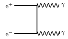
In principle, baryon exchange is very appealing, since it uses for $\overline{\mathrm{N}}\mathrm{N}$ annihilation the same baryon–baryon–meson couplings that enter NN forces. It is not clear, however, whether the form factors can be extrapolated from the NN scattering region to the $\overline{\mathrm{N}}\mathrm{N}$ annihilation region. There is also a warning by Christillin [319] that the exchange of a $\Delta$ or other nucleon resonance leads to a range and a strength comparable to those of nucleon exchange. Hence there is an ambiguity on how the series of exchanges should be truncated, before adjusting the parameters.

However, baryon exchange models have been developed by several authors, in particular the Bonn–Jülich group, see [308, 320], and references therein. These authors treated annihilation “adiabatically”, first by estimating – in their approach – the transition to a few two-meson channels and mimicking the remaining channels by an empirical optical potential. They then gradually increased the number of channels explicitly accounted for. In this framework, one can test the role of various ingredients such as: the coupling constants in the meson–nucleon–nucleon vertices, the associated form factors, the role of final-state interaction, etc. The role of $\Delta$ exchange has also been investigated in this framework [321].

8.5.2 Annihilation range from statistical considerations

Another estimate of the range for annihilation was proposed by Fermi [322]. It is reproduced here in the notation of Amado et al. [323]. The phase-space for annihilation into $n$ particles with momenta ${\vec{p}}_{i}$ and energy $E_{i}$, see Eq. (4.10), is given by integrating

$$\varrho_{n}(s,\{{\vec{p}}_{i}\})=\delta^{4}(\tilde{P}-\tilde{p}_{1}-\cdots\tilde{p}_{n})\prod_{i=1}^{n}{\mathrm{d}^{3}{\vec{p}}_{i}\over 2E_{i}}~{}.$$ (8.13)

The integrals with different $n$ having different dimensions, one should introduce a scale factor $L$ such that the rate for producing $n$ pions reads

$$R(n)={L^{2n}\over n!}\int\varrho_{n}(s,\{{\vec{p}}_{i}\})~{}.$$ (8.14)

Adjusting the average multiplicity $\langle n\rangle=\sum nR(n)/\sum R(n)$ to be 5 gives $L\simeq 1.2\;$fm. This simple reasoning also reproduced the observed variance $\Delta n\simeq 1$ of the multiplicity distribution. A more careful calculation accounting for the $2\pi$ factors of Eq. (4.10) would even increase the range $L$ [323]. Obviously, the scale factor $L$ is related to the size of the fireball from which pions are emitted and thus to $R_{\mathrm{si}}$.

8.5.3 Quark rearrangement

The quark model explains why a baryon and its antiparticle can energetically annihilate by simple quark rearrangement, i.e., why the reaction $({\bar{q}}{\bar{q}}{\bar{q}})+(qqq)\to(\bar{q}q)+(\bar{q}q)+(\bar{q}q)$ can occur at rest. A reasonable phenomenology of both mesons and baryons is, indeed, achieved [324] if it is assumed that the interquark potential obeys the so-called “1/2 rule”

$$V_{\mathrm{qqq}}={1\over 2}\sum_{i<j}V_{\bar{q}q}(r_{ij})~{}.$$ (8.15)

This is obtained by exchanging colour-octets. A linear confinement $V=\lambda r$ for mesons is better generalised as a $Y$-shape interaction for baryons [325]

$$V_{Y}=\lambda\min_{J}(d_{1}+d_{2}+d_{3})~{},$$ (8.16)

where $d_{i}$ is the distance from the quark $i$ to a junction $J$, whose location at minimum corresponds to the well-known Fermat–Torricelli point of elementary triangle geometry. This genuine 3-body interaction is however close to the result for the 1/2 rule, but slightly larger, since [325]

$${1\over 2}(r_{12}+r_{23}+r_{31})\leq\min_{J}(d_{1}+d_{2}+d_{3})\leq{1\over\sqrt{3}}(r_{12}+r_{23}+r_{31})~{}.$$ (8.17)

The variational principle implies that if $V_{\mathrm{qqq}}\geq\sum V_{\bar{q}q}(r_{ij})/2$, then $2M(\mathrm{qqq})\geq 3M(\bar{q}q)$ [326]. Note that quarks and antiquarks are assumed here to have equal masses. If $m(Q)\gg m(q)$, then the inequality can be inverted into $M(\mathrm{qqq})+M(\overline{\mathrm{Q}}\overline{\mathrm{Q}}\overline{\mathrm{Q}})<3M(\overline{\mathrm{Q}}\mathrm{q})$ [327]. Very heavy antibaryons with three units of heavy flavour would not “annihilate” on ordinary matter.

In the quark model, the finite size of annihilation is understood from the composite structure of baryons and mesons. Mesons are produced according to their ability to make a “bridge”, i.e., pick up a quark in N and an antiquark in $\overline{\mathrm{N}}$ [328, 329, 330]. The baryon size governs the spatial spread of the final mesons.

This can seen as follows. A typical transition potential is

$$\langle\Psi_{\mathrm{f}}|{\cal O}|\Psi_{\mathrm{f}}\rangle~{},$$ (8.18)

where the operator ${\cal O}$ correspond to various terms of the interaction Hamiltonian. One gets a good idea of rearrangement by estimating the simple overlap integral corresponding to ${\cal O}=1$. Other matrix elements have similar shape. For describing the initial state, the individual coordinates $\vec{r}_{i}$, corresponding to the labelling of Fig. 22, can be rearranged into

Figure 22: Notation for the rearrangement diagram.

  $${\vec{r}={\vec{r}_{4}+\vec{r}_{5}+\vec{r}_{6}-\vec{r}_{1}-\vec{r}_{2}-\vec{r}_{3}\over\sqrt{6}}~{},\quad} {{}\vec{\rho}_{\overline{\mathrm{N}}}={\vec{r}_{2}-\vec{r}_{1}\over\sqrt{2}}~{},\qquad} {\vec{\lambda}_{\overline{\mathrm{N}}}={2\vec{r}_{3}-\vec{r}_{1}-\vec{r}_{1}\over\sqrt{6}}~{},} {\vec{R}={\vec{r}_{1}+\vec{r}_{2}+\vec{r}_{3}+\vec{r}_{4}+\vec{r}_{5}+\vec{r}_{6}\over\sqrt{6}}~{},\quad} {{}\vec{\rho}_{\mathrm{N}}={\vec{r}_{5}-\vec{r}_{4}\over\sqrt{2}}~{},\qquad} {\vec{\lambda}_{\mathrm{N}}={2\vec{r}_{6}-\vec{r}_{4}-\vec{r}_{5}\over\sqrt{6}}~{},}$$   (8.19)

so that in a harmonic-oscillator model for baryons, the initial wave function reads, in the centre-of-mass

$$\Psi_{\mathrm{i}}=\left({a\over\pi}\right)^{3}\exp\left[-{a\over 2}({\vec{\rho}}_{\overline{\mathrm{N}}}^{\,2}+{\vec{\lambda}}_{\overline{\mathrm{N}}}^{\,2}+{\vec{\rho}}_{\mathrm{N}}^{\,2}+{\vec{\lambda}}_{\mathrm{N}}^{\,2})\right]\,F(\vec{r})~{},$$ (8.20)

assuming a simple factorisation of the relative wave function $F$ and the internal quark or antiquark motion.

Similarly, the final state is described by the internal meson coordinates $\vec{x}_{i}$ and global meson coordinates $\vec{y}_{i}$, $i=1,\,2,\,3$,

$$\vec{x}_{i}={\vec{r}_{i+3}-\vec{r}_{i}\over\sqrt{2}}~{},\qquad\vec{y}_{i}={\vec{r}_{i}+\vec{r}_{i+3}\over\sqrt{2}}~{},$$ (8.21)

and out of the latter, on can built $\vec{R}$ and

$$\vec{\rho}={\vec{y}_{2}-\vec{y}_{1}\over\sqrt{2}}~{},\quad\vec{\lambda}={2\vec{y}_{3}-\vec{y}_{1}-\vec{y}_{2}\over\sqrt{6}}~{},$$ (8.22)

so that, again assuming a harmonic oscillator and factorisation, the final-state wave function reads

$$\Psi_{\mathrm{f}}=\left(b\over\pi\right)^{9/4}\exp\left[-{b\over 2}({\vec{x}}_{1}^{\,2}+{\vec{x}}_{2}^{\,2}+{\vec{x}}_{3}^{\,2})\right]\,G(\vec{\rho},\vec{\lambda})~{}.$$ (8.23)

If one keeps an intermediate set of variables made of $\vec{R}$, $\vec{r}$, $\vec{\rho}$, $\vec{\lambda}$ and

$$\vec{u}={\vec{x}_{2}-\vec{x}_{1}\over\sqrt{2}}={\vec{\rho}_{\mathrm{N}}-\vec{\rho}_{\overline{\mathrm{N}}}\over\sqrt{2}}~{},\quad\vec{v}={2\vec{x}_{3}-\vec{x}_{1}-\vec{x}_{2}\over\sqrt{6}}={\vec{\lambda}_{\mathrm{N}}-\vec{\lambda}_{\overline{\mathrm{N}}}\over\sqrt{2}}~{},$$ (8.24)

one can integrate over these latter variables and get

$$\langle\Psi_{\mathrm{f}}|\Psi_{\mathrm{f}}\rangle={2a^{9/2}b^{15/4}\over\pi^{9/4}(a+b)}\,F(\vec{r})\,G(\vec{\rho},\vec{\lambda})\,\exp\left(-{b{\vec{r}}{}^{\,2}\over 2}\right)\,\exp\left(-{a\over 2}({\vec{\rho}}{}^{\,2}+{\vec{\lambda}}{}^{\,2})\right)~{}.$$ (8.25)

As mentioned earlier, the $\vec{r}$ dependence is governed by the oscillator parameter $b$ of the meson wave functions, while the spatial distribution of the final mesons, described by the coordinates $\vec{\rho}$ and $\vec{\lambda}$, is linked to the baryon size $a$.

This expression (8.25) corresponds to a transition $\overline{\mathrm{N}}\mathrm{N}\to 3$ mesons. If iterated with its conjugate, it gives the contribution to the absorptive part of the $\overline{\mathrm{N}}\mathrm{N}$ amplitude, possibly identified as the driving term of the imaginary part of the optical potential. One gets an exactly separable potential

$$\Im\mathrm{m}[V]\propto\exp(-b{\vec{r}}{}^{\,2}/2)\,\exp(-b\vec{r}{\,}^{\prime 2}/2)~{},$$ (8.26)

acting between an initial $\overline{\mathrm{N}}\mathrm{N}$ wave function $F(\vec{r})$ and a final mesonic wave function $F(\vec{r}{\,}^{\prime})$, in contrast with the local character of optical potentials used in current phenomenological pictures. Green et al. [331, 310] and Ihle et al. [329] went a little further and studied to what extent quark rearrangement can describe a large fraction of the observed annihilation cross-section. The predicted order of magnitude is reasonable, at least in the framework of simple constituent models. This means that quark rearrangement is hardly negligible. It even opens up the possibility of attempting a first study of the systematics of branching ratios [332].

However, to account for two-body modes, kaon production and the detailed features of branching ratios, other quark diagrams have to be included, with some, if not all, incoming quarks and antiquarks annihilating and some quark–antiquark pairs being created in the final state out of the released energy. A phenomenology has been developed, to try to extract from the data the relative importance of the various types of diagrams. Different authors have reached conflicting conclusions, thus illustrating the difficulties of the art of annihilation diagrammatics, which will be presented later in this section.

8.5.4 Annihilation ranges from the Vandermeulen model

The values $R_{\mathrm{so}}=1/(2m_{p})\sim 0.1$ fm for the radius of the annihilation source, and $R_{\mathrm{si}}\sim 1.5$ fm for the average interaction radius are suggested by data on annihilation into $\eta$ and $\eta^{\prime}$. They deserve some comments:

• A small source cannot provide $\ell>0$ orbital angular momenta. Without the Blatt–Weisskopf correction, the branching ratios would scale as $q^{3}$. The momentum for $\omega\eta^{\prime}$ production is only half of the momentum for $\omega\eta$ production. In addition, the $\eta^{\prime}$ has a smaller fraction of $\bar{{n}}{n}$ quarks than the $\eta$. Hence $r_{X}$ should be expected to be about 1/10 while experiments give about 1/2. The angular momentum barrier cannot be large. This is why the $R_{\mathrm{si}}$ in Eq. (8.7) must be large. One could simplify into $R_{\mathrm{si}}=R_{\rm an}=1\,$fm but adopting a larger value for $R_{\mathrm{si}}$ gives a slightly better description of the data.

• A large source cannot provide large linear momenta, as expressed by the term $\exp(-2qR_{\mathrm{so}})$. Only for small $R_{\mathrm{so}}$, the momentum dependence is weak enough to describe simultaneously data on $\bar{\mathrm{p}}\mathrm{p}\to\pi\eta$ and $\bar{\mathrm{p}}\mathrm{p}\to\omega\eta^{\prime}$.

• $R_{\mathrm{so}}$ is small compared to the radii used to fit cross sections [1]. The smallness of the annihilation source $R_{\mathrm{so}}\sim 0.1$ fm underlines the importance of the real part of the interaction: at $R_{\mathrm{si}}\sim 1$ fm strong interactions lead to a strong attraction which focuses the wave function into a region (of size $R_{\mathrm{so}}\sim 0.1$ fm) where annihilation takes place, a scenario often underlined by Shapiro [6].

These results illustrate the hot debate about the annihilation range. Shapiro [333] and others insisted that the annihilation range must be in the order of magnitude of the Compton length of the annihilating baryons, independently of how the annihilating objects are constructed from their constituents. On the other hand, the annihilation range needs to be properly defined. Nucleons are composite particles, as well as mesons. As soon as there is sufficient overlap of the wave functions, rearrangement of quarks can occur and mesons are produced. Thus annihilation sets in at large distances [334].

8.6 Quark diagrams

Figure 23 shows a sample of annihilation diagrams where the flavour flow is represented by lines. A2, A3, R2, R3 are abbreviations to denote quark diagrams with two or three mesons or mesons resonances produced, with or without crossing the lines.

Figure 23: Annihilation (A2, A3) and rearrangement (R2,R3) diagrams for $\overline{\mathrm{N}}\mathrm{N}$ annihilation.

These diagrams are not Feynman diagrams, there is no mathematical prescription as to how to calculate annihilation branching ratios from these pictures. They have to be supplemented by a model providing initial and final state wave-functions, and an operator describing pair creation. So the question arises whether these diagrams can be a useful guide to annihilation processes. The main argument in favour of quark diagrams lies in the dynamical selection rules and the observation, at the end of Sec. 7.7, that the dynamical selection rules are related to the flavour flow.

Diagrams with the same topology might be thought to be equivalent, for instance to those in Fig. 24 where either three mesons are created and rescatter into a resonance or two mesons are produced and one meson undergoes a subsequent decay. In actual model calculations, with constituent wave functions and empirical creation/annihilation operators, the two diagrams are not necessarily equivalent.

Figure 24: Possible mechanisms for $\pi\pi\pi$ production.

8.6.1 Quark–antiquark creation or annihilation

Hadron physics requires more than the “naive quark model”, an oversimplified approximation to QCD, where the number of dressed constituents is frozen, as in ordinary quantum mechanics. A minimal extension has been proposed [335, 336, 337, 338] to account for the decay of meson and baryon resonances. Usually, a “$\bar{q}q$ pair-creation operator” is introduced in an ad-hoc way, its strength is fitted to reproduce a first resonance width, and then the model is (rather successfully) applied to predict all other widths. The calculation of the hadronic widths for, say, $A\to B+C$, contains an overlap integral involving this creation operator, and the wave functions of $A$, $B$ and $C$ computed in a specific quark model. For a review, see the book by Le Yaouanc et al. [336].

In the physics of decaying resonances, the momenta are rather low, so it is not too much of a surprise that a single ansatz can account for the regularities of the observed widths. The current prescription is that $\bar{q}q$ is created with vacuum quantum numbers, i.e., in a ${}^{3}{{\mathrm{P}}}_{0}$ partial wave. This hypothesis is not tested in great detail, since in a decay $A\to B+C$ , there are not too many possibilities for the angular momentum between $B$ and $C$ in the final state. It is thus an audacious enterprise to use the same type of model for describing annihilation: the momentum of the emitted mesons is much larger; the $\bar{q}q$ creation or annihilation operator is required to work more than once; much more freedom is imaginable for the angular momenta, etc. Quark models of annihilation mostly use the ${}^{3}{{\mathrm{P}}}_{0}$ model or a ${}^{3}{{\mathrm{S}}}_{1}$ model, where the $\bar{q}q$ pair has the quantum number of an isoscalar vector, or a combination of both. See, e.g., the discussion by Mandrup et al. [339, 340], Niskanen and Myhrer [309], Dover and Fishbane [341], and Maruyama et al. [307].

8.6.2 Planar and non-planar diagrams

A large fraction of $\bar{\mathrm{p}}\mathrm{p}$ annihilation events, called two-body or quasi-two-body annihilation, produce two primary mesons. These mesons may be unstable and decay with a short lifetime. The reaction $\bar{\mathrm{p}}\mathrm{p}\to\rho\pi$ with $\rho$ decaying into $\pi\pi$ is a typical example. There has been much discussion on whether $\rho\pi$ production is better described by the diagram A2 in Fig. 23, without crossing of quark lines, or by R2, which avoid annihilation and recreation of one quark–antiquark pair but requires crossing of quark lines.

Besides this specific example, attempts have been made to single out a few dominant diagrams, leading to definite predictions for the hierarchy of branching ratios [318]. Guidance was sought from two main sources.

• The OZI rule, as discussed in Sec. 3.3.4 suggests that disconnected diagrams are suppressed. A further step is to assume that only diagrams with planar topology (diagrams that can be drawn on a plane without intersecting lines) are dominant.

• The suppression of disconnected diagrams is unanimously acknowledged to become rigorous in the large $N_{\mathrm{c}}$ limit of QCD, where $N_{\mathrm{c}}$ is the number of colours. However, the question of the suppression of connected but non planar diagrams (such as rearrangement) has been reanalysed by Pirner [342]. His conclusions do not support the claim that planar diagrams dominate.

Models assuming dominance of annihilation diagrams over rearrangement diagrams predict the transition amplitudes $T$ for annihilation into two isovector and into two isoscalar mesons to be the same. For instance, in these models, the rate for $\bar{\mathrm{p}}\mathrm{p}\to\omega\eta$ is similar to $\bar{\mathrm{p}}\mathrm{p}\to\rho\pi$, once some corrections have been applied. One correction is required for the $\bar{{s}}{s}$ component in the $\eta$ wave function. Another correction is the Vandermeulen factor $F_{\ell}(q)$ (see Eq. 8.6). The dynamically corrected ratios ${\rm DR}$ are given in Table 42, with $\Theta=\Theta_{\rm PS}-\Theta_{\rm id}+\pi/2$ and $\Theta_{\rm PS}=-15.9^{\circ}$ (see Eq. 8.12).

The ratios in Table 42 are largely incompatible with 1, whilst some have the right order of magnitude. With this warning, Table 42 could support the hypothesis that planar diagrams might in some cases drive the leading contribution to two-meson annihilation.

Table 42: Ratios of dynamically corrected annihilation frequencies for $\bar{\mathrm{p}}\mathrm{p}$ annihilation into two isoscalar and two isovector mesons.

${\displaystyle 1\over\displaystyle\cos^{2}\Theta}{\displaystyle{\rm DR}(\bar{\mathrm{p}}\mathrm{p}\to\eta\omega)\over\displaystyle{\rm DR}(\bar{\mathrm{p}}\mathrm{p}\to\rho^{0}\pi^{0})}$	=	$1.77\pm\ 0.10$	${\displaystyle{\rm DR}(\bar{\mathrm{p}}\mathrm{p}\to\rho^{0}\rho^{0})\over\displaystyle{\rm DR}(\bar{\mathrm{p}}\mathrm{p}\to\omega\omega)}$	=	$0.04\pm\ 0.04$
$\cos^{4}\Theta$ ${\displaystyle{\rm DR}(\bar{\mathrm{p}}\mathrm{p}\to\pi^{0}\pi^{0})\over\displaystyle{\rm DR}(\bar{\mathrm{p}}\mathrm{p}\to\eta\eta)}$	=	$1.67\pm\ 0.14$	${\displaystyle 1\over\displaystyle\cos^{2}\Theta}{\displaystyle{\rm DR}(\bar{\mathrm{p}}\mathrm{p}\to\eta{\mathrm{f}}_{2}(1270))\over\displaystyle{\rm DR}(\bar{\mathrm{p}}\mathrm{p}\to\pi^{0}{\mathrm{a}}_{2}(1320))}$	$<$	$0.05\quad\ (1\sigma)$

8.6.3 Strangeness production

In models where A2 is small compared to R2, a small fraction of events contain a pair of kaons. On the other hand, if A2 is the leading mechanism of annihilation, and if SU(3) symmetry is approximately valid, a very large number of kaons is expected. This is a serious problem for models based on A2, since the overall yield of strange particles is only about $5\%$.

This is why, in models where A2 and other planar diagrams are assumed to dominate annihilation, it is crucial to introduce an explicit SU(3) breaking, in the form of a suppression factor $\lambda$ for $\bar{{s}}{s}$-creation, compared to $\bar{{n}}{n}$. A value $\lambda=1$ corresponds to the SU(3) limit. To push the fraction of hidden strangeness production close to the experimental value, models based on planar diagrams need a value as low as $\lambda\sim 0.1$.

A theoretical foundation for $\bar{{s}}{s}$ suppression was given by Dosch and Gromes [343], who showed that $\bar{{s}}{s}$ could be very much suppressed just above threshold, by a kind of tunnelling effect. In the hadronisation following high-energy reactions, the production of strange quarks is also reduced compared to the production of up and down quarks. This is why fragmentation models incorporate a strangeness suppression factor $\lambda$. It increases with energy from values as low as 0.1 at a few GeV to $\sim 0.3$ at 30 GeV [344]. $\bar{\mathrm{p}}\mathrm{p}$ annihilation being a soft process, a value $\lambda\sim 0.1$ seems not unreasonable. Such a low value has decisive consequences for the interpretation of annihilation data. If $\lambda\sim 0.1$ were true, SU(3) symmetry would be dramatically broken. The suppression would result in heavier kaon resonances being more suppressed than lighter kaons, and also $\mathrm{\overline{K}K}$ dramatically increasing in annihilation in flight as compared to annihilation at rest. Hence there is a possibility of understanding the data by the dominance of annihilation diagrams supplemented by $\bar{{s}}{s}$ suppression.

Fragmentation of hadrons is, however, a rather indirect way to address the question of $\bar{{s}}{s}$ suppression at low energies. Meson decays may be a better guide. The tensor meson ${\mathrm{a}}_{2}(1320)$ has dominant decay modes into $\rho\pi$, $\eta\pi$ and into $\mathrm{K}\overline{\mathrm{K}}{}$. SU(3) relates the decays into $\eta\pi$ and into $\mathrm{K}\overline{\mathrm{K}}{}$. Their ratio, and the decay branching ratios of all tensor mesons, are fully compatible with only small SU(3) symmetry breaking. The authors of Ref. [249] fitted 16 decay modes of tensor mesons with SU(3) amplitudes allowing for $\bar{{s}}{s}$ suppression. They found $\lambda=0.8\pm 0.2$: data on tensor meson decays are compatible with SU(3) and rule out a substantial SU(3) symmetry breaking.

Table 43: Selected $\rm J/\psi$ decays probing SU(3) symmetry. Data are taken from Ref. [237]. The experimental value is shown, and then corrected for a phase-space factor $p^{2\ell+1}$, where $p$ is the momentum, and $\ell$ the angular momentum in the final state. The units for BR/$p^{2\ell+1}$ are irrelevant. For isospin multiplets, we assume normal weights for each charge state or average over the data, and display this average, contrary to [237] where, e.g., $\rho\pi$ means the sum of the three channels.

Channel	BR ($10^{-3}$)	BR/$p^{2\ell+1}$		Channel	BR ($10^{-3}$)	BR/$p^{2\ell+1}$
$\rm p\bar{p}$	$2.12\pm 0.10$	1.7		$\rho\pi$	$4.2\ \pm 0.5\$	1.7
$\rm n\bar{n}$	$2.2\ \pm 0.4\$	1.5		$\omega\eta$	$1.58\pm 0.16$	0.6
$\Lambda\overline{\Lambda}$	$1.30\pm 0.12$	1.3		$\mathrm{K}^{*}\overline{\mathrm{K}}{}+{\rm c.c.}$	$2.3\ \pm 0.2\$	0.9
$\Sigma\overline{\Sigma}$	$1.27\pm 0.17$	1.3		$\pi\pi$	$0.15\pm 0.02$	0.04
$\Xi\overline{\Xi}$	$0.9\ \pm 0.2\$	1.1		$\mathrm{K}\overline{\mathrm{K}}{}$	$0.19\pm 0.03$	0.06
$\Delta\overline{\Delta}$	$1.10\pm 0.29$	1.2		${\mathrm{a}}_{2}(1320)$$\rho$	$3.6\ \pm 0.7\$	3.2
$\Sigma^{*}\overline{\Sigma}{}^{*}$	$0.52\pm 0.07$	0.8		${\mathrm{f}}_{2}(1270)\omega$	$4.3\ \pm 0.6\$	3.6
				$\mathrm{K}_{2}^{*}\mathrm{K}$	$3.4\ \pm 1.3\$	2.4

The Mark III Collaboration studied J/$\psi$ decays into a vector and a pseudoscalar meson in order to find ”inert” or gluonic components in the $\eta$ and $\eta^{\prime}$ wave functions. The result was negative. One of the (rather numerous) parameters was the suppression of $\bar{{s}}{s}$ pair creation compared to the creation of $\bar{{u}}{u}$ or $\bar{{d}}{d}$ pairs. From their fit a value $\lambda=0.8$ was deduced [345].

We looked for strangeness suppression in J/$\psi$ decays into baryons, into $\rm p\bar{p}$, $\rm n\bar{n}$, $\Lambda\overline{\Lambda}$, $\Sigma\overline{\Sigma}$, $\Xi\overline{\Xi}$, $\Delta\overline{\Delta}$, and $\Sigma^{*}\overline{\Sigma}{}^{*}$. After correcting for phase space (i.e., after division by the respective decay momenta) the squared invariant couplings are similar in size, but scale with $0.75^{n_{s}}$ where $n_{s}$ is the number of $\bar{{s}}{s}$ pairs created. The creation of a second $s\bar{s}$ pair in $\Xi\overline{\Xi}$ is certainly a non-perturbative process but still governed by $\lambda\sim 0.75$!

In short, the physics of tensor mesons and charmonium decay does not support $\bar{{s}}{s}$ suppression, and hence calls, in the case of $\overline{\mathrm{N}}\mathrm{N}$ annihilation, for an important role of non-planar, rearrangement diagrams.

Perhaps strangeness production in $\overline{\mathrm{N}}\mathrm{N}$ cannot be explained in a simple uniform manner and should instead be examined for each type of final state. Table 44 compares (dynamically corrected) branching ratios for annihilation into two strange mesons with those for annihilation into two isovector mesons. The data are grouped into processes in which the two vector mesons come from isoscalar ($D$-coupling) and isovector ($F$-coupling) protonium states. $D$ or $F$ coupling belong to standard SU(3) notation [237].

The ratios with $D$- and $F$-coupling differ remarkably while being internally compatible. There is an astonishing consistency between these ratios when processes of the same SU(3) structure are compared. Again, the flavour flow is responsible for gross features of two-body annihilation processes.

The ratios with $F$-coupling suggest that A2 might be the relevant quark line diagram, possibly with a ‘penalty factor’ $(\sim 0.5)$ for producing a $s\bar{s}$ pair. Then the rearrangement diagram R2 must contribute strongly to the production of two isovector mesons from isoscalar initial states. To conclude, it seems that the data on strangeness production support a scenario where rearrangement diagrams are important.

The problem of strangeness production is not restricted to the question of the relative importance of A2 vs. R2 diagrams. Another mechanism has been proposed by Ellis et al. [346], where strange quarks and antiquarks are extracted from the nucleon or antinucleon sea, leading to specific signatures, for instance for the spin effects in $\bar{\mathrm{p}}\mathrm{p}\to\overline{\Lambda}\Lambda$, and for the violation of the OZI rule (on which more in the next subsection). Holinde et al. [347] suggested a possible role of initial-state interaction, via $\overline{\mathrm{N}}\mathrm{N}\to\overline{Y}Y$, to describe the $\bar{\mathrm{p}}\mathrm{p}\to\phi\phi$ annihilation in flight. The mechanism can also be applied to a violation of the OZI rule, since the hyperons $Y$ and $\overline{Y}$ can produce a $\phi$ together with light mesons by simple rearrangement.

Table 44: Dynamically corrected branching ratios for annihilation into strange mesons and into two isovector mesons in the final state for different SU(3) flavour couplings. A “$+\mathrm{c.c.}$” is implied for every final state with a $\mathrm{K}{}^{*}$ or $\mathrm{K}_{2}^{*}$.

$D$-coupling				$F$-coupling
${\displaystyle{\rm DR}\left({}^{3}{{\mathrm{P}}}_{0}\to\mathrm{K}\overline{\mathrm{K}}{}\right)\over\displaystyle{\rm DR}\left({}^{1,3}{{\mathrm{P}}}_{0}\to\pi\pi\right)}$	=	$0.047\pm\ 0.004$		${\displaystyle{\rm DR}\left({}^{3}{{\mathrm{S}}}_{1}\to\mathrm{K}\overline{\mathrm{K}}{}\right)\over\displaystyle{\rm DR}\left({}^{3,3}{{\mathrm{S}}}_{1}\to\pi\pi\right)}$	=	$1.00\pm\ 0.20$
${\displaystyle{\rm DR}\left({}^{3}{{\mathrm{S}}}_{1}\to\mathrm{K}^{*}\overline{\mathrm{K}}{}\right)\over\displaystyle{\rm DR}\left({}^{1,3}{{\mathrm{S}}}_{1}\to\rho\pi\right)}$	=	$0.049\pm\ 0.008$		${\displaystyle{\rm DR}\left({}^{1}{{\mathrm{S}}}_{0}\to\mathrm{K}^{*}\overline{\mathrm{K}}{}\right)\over\displaystyle{\rm DR}\left({}^{3,1}{{\mathrm{S}}}_{0}\to\rho\pi\right)}$	=	$0.58\pm\ 0.13$
${\displaystyle{\rm DR}\left({}^{1}{{\mathrm{S}}}_{0}\to\mathrm{K}\mathrm{K}{}^{*}_{2}(1430)\right)\over\displaystyle{\rm DR}\left({}^{1,3}{{\mathrm{S}}}_{1}\to{\mathrm{a}}_{2}(1320)\pi\right)}$	=	$0.033\pm\ 0.010$		${\displaystyle{\rm DR}\left({}^{3}{{\mathrm{S}}}_{1}\to\mathrm{K}\mathrm{K}{}^{*}_{2}(1430)\right)\over\displaystyle{\rm DR}\left({}^{3,3}{{\mathrm{S}}}_{1}\to{\mathrm{a}}_{2}(1320)\pi\right)}$	=	$0.34\pm\ 0.14$

8.7 Violation of the OZI rule

The quark-line rule, or OZI rule, has already been introduced for mesons, see sec. 3.3.4. To first order, the rule forbids production of $\phi$ mesons from initial systems like $\bar{\mathrm{p}}\mathrm{p}$ with up and down quarks only. The vector meson mixing angle, $\Theta_{V}=39^{\circ}$ for the quadratic GMO mass formula, allows for the small $\phi\to\pi^{+}\pi^{-}\pi^{0}$ decay rate, and also $\phi$ production from $\bar{\mathrm{p}}\mathrm{p}$ is permitted with an expected ratio

$$d_{X}({\rm vector,expected})=\tan^{2}(\Theta_{V}-\Theta_{\rm id})=0.004~{},$$ (8.27)

where $d_{X}({\rm vector})$ is defined as the ratio of the dynamically corrected annihilation frequencies

$$d_{X}({\rm vector})={{\rm DR}(\bar{\mathrm{p}}\mathrm{p}\to X\phi)\over{\rm DR}(\bar{\mathrm{p}}\mathrm{p}\to X\omega)}~{},$$ (8.28)

while the $r_{X}(\rm vector)$ are the corresponding ratios without dynamical corrections. The ratios $r_{X}$ and $d_{X}$ are defined analogously for the tensor mesons ${\mathrm{f}_{2}}(1270)$ and ${\mathrm{f}_{2}}(1525)$.

Different analyses of bubble chamber data gave results in the range from 0.07 to 0.23 for the ratio of annihilation frequencies $\mathrm{AF}(\bar{\mathrm{p}}N\to\pi\phi)$ to $\mathrm{AF}(\bar{\mathrm{p}}N\to\pi\omega)$ [348]. Based on a selection of results, a mean value $0.085\pm 0.030$ was given in [124]. Obviously $\phi$ production is much stronger than the anticipated ratio $0.004$ suggests.

At LEAR, $\phi$ production was studied by the Asterix [124], Obelix [132, 147, 148, 154], and Crystal Barrel collaborations [170, 176]. In Table 45 we give ratios $r_{X}({\rm nonet})$ and $d_{X}({\rm nonet})$ for $X=\pi^{0}$ and $X=\eta$ from the two initial states ${}^{3}{{\mathrm{S}}}_{1}$ and ${}^{1}{{\mathrm{P}}}_{1}$.

Table 45: Ratios of $\phi/\omega$ and $\mathrm{f}_{2}(1525)/\mathrm{f}_{2}(1270)$ production. Given are the $\bar{\mathrm{p}}\mathrm{p}$ initial state, the recoil meson, the ratio without and with dynamical corrections, and the ratio expected from the nonet mixing angle. In the last column, the isospin component is given which gives the dominant contribution to the corresponding final states with kaons.

$\bar{\mathrm{p}}\mathrm{p}$	$X$	$r_{X}({\rm vector})$	$d_{X}({\rm vector})$	From GMO	$\mathrm{K}^{*}\overline{\mathrm{K}}{}$
${}^{3,3}{{\mathrm{S}}}_{1}$	$\pi^{0}$	0.099$\pm$0.012	0.105$\pm$0.013	0.004	$I=1$
${}^{1,3}{{\mathrm{S}}}_{1}$	$\eta$	0.0035$\pm$0.0009	0.0038$\pm$0.0010	0.004	$I=1$
${}^{3,1}{{\mathrm{P}}}_{1}$	$\pi^{0}$	0.005$\pm$0.009	0.005$\pm$0.009	0.004	$I=0$
${}^{1,1}{{\mathrm{P}}}_{1}$	$\eta$	0.10$\pm$0.07	0.12$\pm$0.09	0.004	$I=0$
$\bar{\mathrm{p}}\mathrm{p}$	$X$	$r_{X}({\rm tensor})$	$d_{X}({\rm tensor})$	From GMO	$\mathrm{K}^{*}_{2}\overline{\mathrm{K}}{}$
${}^{3,1}{{\mathrm{S}}}_{0}$	$\pi^{0}$	0.020$\pm$0.004	0.025$\pm$0.005	0.012	$I=0$
$\bar{\mathrm{p}}\mathrm{p}$	$X$	$r_{X}({\rm vector})$	$d_{X}({\rm vector})$	From GMO	$\mathrm{K}^{*}\overline{\mathrm{K}}{}^{*}$
${}^{3,1}{{\mathrm{S}}}_{0}$	$\rho$	0.018$\pm$0.007	0.030$\pm$0.010	0.004	both
${}^{1,1}{{\mathrm{S}}}_{0}$	$\omega$	0.0095$\pm$0.0035	0.017$\pm$0.006	0.004	both
${}^{1}{{\mathrm{S}}}_{0}$	$\gamma$	0.25$\pm$0.09	0.026$\pm$0.09	0.004	both

The ratios vary over a wide range: the $\bar{\mathrm{p}}\mathrm{p}$ annihilation frequencies from the ${}^{3}{{\mathrm{S}}}_{1}$ state to $\phi\eta$, from the ${}^{1}{{\mathrm{P}}}_{1}$ state to $\phi\pi$, and the frequency to $\mathrm{f}_{2}(1525)\pi$ are all of the order of magnitude expected from the meson nonet mixing angles. A few processes give a moderately large $\phi$ production rate like $\phi\rho$ and $\phi\omega$. For some reactions however, the OZI violation is really large, the $\phi/\omega$ ratio being about $10\%$ or larger.

Three interpretations of this large excess of $\phi$ production compared to $\omega$ production have been pursued. Figure 25 sketches the three scenarios.

Figure 25: Diagrams which could contribute to $\phi$ production: as shake-off of hidden $\bar{{s}}{s}$ pairs in the nucleon wave function, via rescattering of Kaons from secondary decays, and from formation of four-quark exotic states.

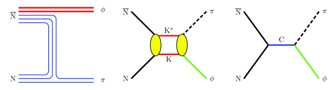
Dover and Fishbane [348] link the excess in $\phi$ production to the production of four-quark exotics with hidden strangeness ($qs\bar{q}\bar{s}$), e.g., to the tail of the $C(1480)$ meson [349].

The nucleon wave function is known to contain an $\bar{{s}}{s}$ component. This is evident from deep inelastic scattering [350] or from the so-called $\pi$-nucleon $\sigma$ term $\sigma_{\rm\pi N}$ [351]. There is no guarantee however that virtual $\bar{q}q$ pairs may be shaken off in an OZI rule violating diagram. If this is assumed, the sharp selectivity of the processes leading to large OZI rule violating effects can potentially be understood [346, 352] as originating from the $\bar{{s}}{s}$ component being negatively polarized.

The PSI group studied OZI rule violating effects in $\overline{\mathrm{N}}\mathrm{N}$ annihilation in a series of papers [353, 354, 355]. See, also, [356, 357, 358]. The large $\pi\phi$ annihilation frequencies were interpreted by rescattering into $\phi$ mesons of $\mathrm{K}\overline{\mathrm{K}}{}$ pairs from $\mathrm{K}\overline{\mathrm{K}}{}^{*}+\mathrm{K}^{*}\overline{\mathrm{K}}{}$ annihilation and or $\rho\pi$ rescattering from $\rho^{+}\rho^{-}$. The large rate for $\gamma\phi$ channel was understood as the effect of $\rho\phi$ and $\omega\phi$ production, and vector meson dominance. The study was extended in [359] to include $\phi\pi^{+}\pi^{-}$ production in $\bar{\mathrm{p}}\mathrm{p}$ annihilation at rest and in flight.

We notice that the ratios $r_{X}$ and $d_{X}$ are large when the $\phi$ and $\omega$ are produced from the isospin component which gives a large contribution to kaonic final states. Rescattering of, e.g., $\mathrm{K}\overline{\mathrm{K}}{}$ in the $\mathrm{K}^{*}\overline{\mathrm{K}}{}$ final state is certainly proportional to the frequency with which $\mathrm{K}^{*}\overline{\mathrm{K}}{}$ with the correct isospin is produced. Indeed, the OZI violation is found to be correlated with the $\mathrm{K}^{*}\overline{\mathrm{K}}{}$ production strength of the required isospin. This observation supports the rescattering interpretation of the strong OZI rule violation. As emphasized in [352], there are more processes in which OZI rule violating effects can be studied and possibly linked to a hidden $\bar{{s}}{s}$ component in the $\overline{\mathrm{N}}\mathrm{N}$ wave function.

Decays of the J/$\psi$ can help to elucidate the problem further. A sample is given in Table 46. The J/$\psi$ wave function has little hidden strangeness, and any $\pi\phi$ production must be due to rescattering. In reversing the argument, the absence of $\pi\phi$ in J/$\psi$ decays could possibly be interpreted as evidence that the large OZI rule violating in $\overline{\mathrm{N}}\mathrm{N}$ annihilation must come from the nucleon wave function.

Table 46: Selected decays modes of J$/\psi$

J/$\psi\to$	$\eta\omega$	$\pi\omega$	$\pi\phi$	$\rm K^{*}K$
Rate $(10^{-4})$	$15.8\pm 1.6$	$4.2\pm 0.6$	$<$0.068	$92\pm 6$

From the $\eta\omega/\pi\omega$ ratio, isospin violation can be estimated to occur at the 14% level. The $\mathrm{K}^{*}\overline{\mathrm{K}}{}$ final state was not analysed to identify isospin breaking effects; however a $\mathrm{K}^{*}\mathrm{K}\,(I=1)$ contribution of more than $10^{-3}$ can be expected. Rescattering may then lead to $\pi\phi$ production at a detectable level.

The problem was studied in [360] using a dispersion theoretical approach. The interpretation of large $\phi\pi$ frequency in $\bar{\mathrm{p}}\mathrm{p}$ annihilation as an effect of rescattering was confirmed. The low $\phi\pi$ production in J/$\psi$ decays is due to its larger phase space, and is compatible with the rescattering mechanism for OZI rule violating effects.

8.8 Flavour flow and flavour symmetry

Support for the use of quark-line diagrams can be found by comparing branching ratios for annihilation into specific two-body final states. In Table 47, we compare dynamically corrected annihilation frequencies DR, using Eq. (8.6). The numerators correspond to final states with one isovector and one isoscalar meson, and the denominators to annihilation into two isovector or two isoscalar mesons.

Table 47: Ratios of dynamically corrected annihilation frequencies DR into an isovector and an isoscalar meson compared to production of two isoscalar or two isovector mesons. Bose symmetry is taken into account.

${\displaystyle 1\over\displaystyle 2\cos^{2}\Theta}{\displaystyle{\rm DR}(\bar{\mathrm{p}}\mathrm{p}\to\pi^{0}\eta)\over\displaystyle{\rm DR}(\bar{\mathrm{p}}\mathrm{p}\to\pi^{0}\pi^{0})}=0.24\pm 0.08$	${\displaystyle 1\over\displaystyle 2\sin^{2}\Theta}{\displaystyle{\rm DR}(\bar{\mathrm{p}}\mathrm{p}\to\pi^{0}\eta^{\prime})\over\displaystyle{\rm DR}(\bar{\mathrm{p}}\mathrm{p}\to\pi^{0}\pi^{0})}=0.24\pm 0.7\phantom{0}$
${\displaystyle\cos^{2}\Theta\over\displaystyle 2}{\displaystyle{\rm DR}(\bar{\mathrm{p}}\mathrm{p}\to\pi^{0}\eta)\over\displaystyle{\rm DR}(\bar{\mathrm{p}}\mathrm{p}\to\eta\eta)}=0.40\pm 0.10$	${\displaystyle\cos^{4}\Theta\over\displaystyle 2\sin^{2}\Theta}{\displaystyle{\rm DR}(\bar{\mathrm{p}}\mathrm{p}\to\pi^{0}\eta^{\prime})\over\displaystyle{\rm DR}(\bar{\mathrm{p}}\mathrm{p}\to\eta\eta)}=0.48\pm 0.14$
${\displaystyle\sin^{2}\Theta\over\displaystyle 2}{\displaystyle{\rm DR}(\bar{\mathrm{p}}\mathrm{p}\to\pi^{0}\eta)\over\displaystyle{\rm DR}(\bar{\mathrm{p}}\mathrm{p}\to\eta\eta^{\prime})}=0.31\pm 0.10$	$\cos^{2}\Theta\,{\displaystyle{\rm DR}(\bar{\mathrm{p}}\mathrm{p}\to\pi^{0}\eta^{\prime})\over\displaystyle{\rm DR}(\bar{\mathrm{p}}\mathrm{p}\to\eta\eta^{\prime})}=0.39\pm 0.06$
${\displaystyle 1\over\displaystyle\cos^{2}\Theta}{\displaystyle{\rm DR}(\bar{\mathrm{p}}\mathrm{p}\to\rho^{0}\eta)\over\displaystyle{\rm DR}(\bar{\mathrm{p}}\mathrm{p}\to\rho^{0}\pi^{0})}=0.40\pm 0.11$	${\displaystyle 1\over\displaystyle\sin^{2}\Theta}{\displaystyle{\rm DR}(\bar{\mathrm{p}}\mathrm{p}\to\rho^{0}\eta^{\prime})\over\displaystyle{\rm DR}(\bar{\mathrm{p}}\mathrm{p}\to\rho^{0}\pi^{0})}=0.45\pm 0.13$
${\displaystyle{\rm DR}(\bar{\mathrm{p}}\mathrm{p}\to\rho^{0}\eta)\over\displaystyle{\rm DR}(\bar{\mathrm{p}}\mathrm{p}\to\omega\eta)}=0.23\pm 0.06$	${\displaystyle\cos^{2}\Theta\over\displaystyle\sin^{2}\Theta}{\displaystyle{\rm DR}(\bar{\mathrm{p}}\mathrm{p}\to\rho^{0}\eta^{\prime})\over\displaystyle{\rm DR}(\bar{\mathrm{p}}\mathrm{p}\to\omega\eta)}=0.26\pm 0.10$
${\displaystyle{\rm DR}(\bar{\mathrm{p}}\mathrm{p}\to\rho^{0}\eta^{\prime})\over\displaystyle{\rm DR}(\bar{\mathrm{p}}\mathrm{p}\to\omega\eta^{\prime})}=0.18\pm 0.06$	${\displaystyle{\rm DR}(\bar{\mathrm{p}}\mathrm{p}\to\rho^{0}\eta^{\prime})\over\displaystyle{\rm DR}(\bar{\mathrm{p}}\mathrm{p}\to\omega\eta^{\prime})}=0.18\pm 0.06$
${\displaystyle{\rm DR}(\bar{\mathrm{p}}\mathrm{p}\to\omega\pi^{0})\over\displaystyle{\rm DR}(\bar{\mathrm{p}}\mathrm{p}\to\rho^{0}\pi^{0})}=0.41\pm 0.06$	$\cos^{2}\Theta\,{\displaystyle{\rm DR}(\bar{\mathrm{p}}\mathrm{p}\to\omega\pi^{0})\over\displaystyle{\rm DR}(\bar{\mathrm{p}}\mathrm{p}\to\omega\eta)}=0.23\pm 0.06$
$\sin^{2}\Theta\,{\displaystyle{\rm DR}(\bar{\mathrm{p}}\mathrm{p}\to\omega\pi^{0})\over\displaystyle{\rm DR}(\bar{\mathrm{p}}\mathrm{p}\to\omega\eta^{\prime})}=0.18\pm 0.07$	${\displaystyle{\rm DR}(\bar{\mathrm{p}}\mathrm{p}\to{\mathrm{f}}_{2}(1270)\pi^{0})\over\displaystyle{\rm DR}(\bar{\mathrm{p}}\mathrm{p}\to{\mathrm{a}}_{2}(1320)\pi^{0})}=0.53\pm 0.09$

The ratios require some corrections. In the process $\bar{\mathrm{p}}\mathrm{p}\to\pi\eta$, the initial $\bar{\mathrm{p}}\mathrm{p}$ system couples only to the $\bar{{n}}{n}$ component and not to the $\bar{{s}}{s}$ component. The OZI rule reduces the amplitude for this process by $\cos\Theta$, and the branching ratio by $\cos^{2}\Theta$. Correspondingly, $\bar{\mathrm{p}}\mathrm{p}\to\pi\eta^{\prime}$ is reduced by $\sin^{2}\Theta$, where $\Theta$ is defined in Eq.(3.7). We use $\cos^{2}\Theta=0.65\pm 0.07$ and $\sin^{2}\Theta=0.35\pm 0.07$.

The table reveals a surprise: most results are about compatible with each other, except for those containing the DR for $\omega\eta^{\prime}$ (which are too large). The mean value of those ratios gives $0.29\pm 0.03$. with a $\chi^{2}/N_{F}=2$. There is no a priori reason why these ratios should be similar. The two final states $\pi^{0}\eta$ and $\pi^{0}\pi^{0}$ are produced from the ${}^{3}{{\mathrm{P}}}_{0}$ initial state, $\rho\eta$ and $\omega\eta$ from ${}^{3}{{\mathrm{S}}}_{1}$, ${\mathrm{f}}_{2}(1270)$$\pi^{0}$ and ${\mathrm{a}}_{2}(1320)$$\pi^{0}$ from ${}^{1}{{\mathrm{S}}}_{0}$. Table 47 includes final states with two light mesons like $\pi$ and $\eta$, or with two massive mesons like $\omega$ and $\rho$; the ratio is formed using pseudoscalar, vector and tensor mesons in arbitrary combinations. In some cases, broad mesons are only in the numerator, in others only in the denominator. Obviously, the flavour content and the flavour coupling are the decisive ingredients. Table 47 supports the conjecture made in Sec. 7.7 that the flavour flow has a decisive impact on annihilation dynamics.

In Table 47, the two annihilation modes $\bar{\mathrm{p}}\mathrm{p}\to\rho^{0}\rho^{0}$ and $\bar{\mathrm{p}}\mathrm{p}\to\eta$${\mathrm{f}}_{2}(1270)$  are excluded. The frequency for annihilation into $\bar{\mathrm{p}}\mathrm{p}\to\rho^{0}\rho^{0}$ is compatible with zero, and there is no known reason for this effect. The reaction $\bar{\mathrm{p}}\mathrm{p}\to\eta{\mathrm{f}}_{2}(1270)$ needs $\ell=2$ and is very close to threshold; the measured frequency is compatible with zero but is also expected to be small.

8.8.1 SU(3): quark-line rule, $s$-channel resonances and baryon exchange

As we have seen $\bar{\mathrm{p}}\mathrm{p}$ annihilation can be discussed in rather different languages. Quark models describe annihilation in terms of planar and non-planar diagrams (often called annihilation and rearrangement diagrams). On the other hand, $\bar{\mathrm{p}}\mathrm{p}$ annihilation may prefer to proceed via a few $s$-channel resonances (e.g., by mixing between the $\bar{\mathrm{p}}\mathrm{p}$ system and $(\bar{q}\bar{q}qq)$ states close in mass). In this case, a description in terms of $s$-channel amplitudes may be more appropriate. Or, alternatively, baryons and mesons might be the relevant degrees of freedom, and $\bar{\mathrm{p}}\mathrm{p}$ annihilation could be most efficiently described by baryon exchange amplitudes. Figure 26 visualises the different approaches.

Figure 26: Annihilation of protons and antiprotons in different coupling schemes. From left to right: the quark line coupling depicting the flavour flux, the $s$-channel coupling with meson formation in the $s$-channel, and baryon exchange coupling where baryons are exchanged in the $t$-channel.

The question to be addressed is which scheme is best suited to incorporate the most important aspects of annihilation, and in particular, whether dynamical selection rules find a natural interpretation in one of the three coupling schemes. The three descriptions are related by unitary matrices which were developed in [361].

Figure 26 shows for each coupling scheme two basic diagrams. Their meaning is illustrated using the quark line coupling scheme. The two outgoing mesons can be symmetric or antisymmetric with respect to their exchange leading to a doubling of diagrams. In any diagram, one antiquark and one quark reach the final state as ‘spectators’. The spectators can be either $(u,\bar{u})$ or $(d,\bar{d})$, again leading to a doubling of diagrams. Hence 8 diagrams are needed to describe the annihilation process. These are shown in figure 27. In case of two mesons in the final state belonging to the same multiplet (e.g. for annihilation into two pseudoscalar mesons), the generalised Pauli principle requires R${}^{+}_{3}$ to vanish.

Figure 27: Explicit representation of quark-line amplitudes of all independent couplings in the quark-line scheme. Pairs of (anti-)quarks antisymmetric with respect to their exchange are connected by small loops.

For a quantitative analysis we use the dynamically corrected branching ratios of Table 41. These should be related to the squared SU(3) transition matrix elements. In the fits we use a strangeness suppression factor $\lambda=0.7$ to $0.8$. The results do not depend critically on this assumption. A SU(3) error of 20% is introduced. The latter is added quadratically to the experimental errors of Table 41.

All three coupling schemes allow us to fit the data with identical $\chi^{2}$. There are 10 measured branching ratios for annihilation into two pseudoscalar mesons and 11 for annihilation into a vector and a pseudoscalar meson, 7 amplitudes in the former case and 8 in the latter one. Since the pseudoscalar mixing angle has been fixed from these data (Eq. 8.12), the number of degrees of freedom is 2 in both cases. These two sets of branching ratios are fitted with $\chi^{2}=1.3$ For annihilation into a pseudoscalar and a tensor meson, there are only 8 data points and 8 amplitudes; the data are reproduced with $\chi^{2}=0$. The three coupling schemes give identical descriptions of the data. Even within one coupling scheme, different solutions exist with identical or similar $\chi^{2}$. Hence care has to be taken in interpreting the results.

8.8.2 The quark coupling scheme

Figure 27 shows the decomposition of the quark coupling scheme. There are 8 amplitudes which may be fit to the values given in Table 48,

Table 48: Best-fit values for the amplitudes in the quark coupling scheme.

	$\rm A^{+}_{1}$	$\rm A^{+}_{2}$	$\rm R^{+}_{1}$	$\rm R^{+}_{2}$	$\rm R^{+}_{3}$	$\rm A^{-}_{1}$	$\rm A^{-}_{2}$	$\rm R^{-}_{1}$
PS–PS	1.6	$-2.1$	9.7	$-0.3$	-	1.4	$-1.5$	1.2
PS–V	2.3	$-1.9$	10.9	1.2	$-3.9$	1.1	$-1.8$	$-1.6$
PS–T	1.3	$-1.8$	8.9	$-2.8$	$-1.0$	0.8	$-1.5$	$-1.8$

where a positive sign has been chosen for the amplitudes $\rm A^{\pm}_{1}$. The largest contribution is given by $\rm R^{+}_{1}$. Before discussing the meaning and significance of this result, a comment is made concerning the amplitudes $\rm A^{\pm}_{1}$ and $\rm A^{\pm}_{2}$. They have opposite signs and are about equal in amplitude. The approximate relations $\rm A^{\pm}_{1}+A^{\pm}_{2}\simeq 0$ hold for all five annihilation processes from initial S-states. For annihilation into two pseudoscalar meson, the data are also approximately compatible with this relation with an alternative solution where $\rm|A^{+}_{1}|\gg|A^{+}_{2}|$. Setting $\rm A^{\pm}_{1}+A^{\pm}_{2}=0$ substantially helps further discussion: annihilation into two isovector mesons (first line in Table 41) is given by the SU(3) matrix element $\rm|2A^{+}_{1}+2A^{+}_{2}+R^{+}_{1}|^{2}$. $\rm R^{+}_{1}$ can be chosen positive or negative; for $\rm A^{+}_{1}+A^{+}_{2}\neq 0$ two values are found; both are large but differ in the precise number. Only for $\rm A^{+}_{1}+A^{+}_{2}=0$, does $\rm R^{+}_{1}$ have a unique value. As long as the interest is in a qualitative understanding, it suffices to state that rearrangement diagrams give a substantial contribution to annihilation and should not be neglected. This statement is compatible with the findings presented above (see Sec. 8.5.3).

Among the rearrangement diagrams, $\rm R^{+}_{1}$ plays the dominant role. This result has to be interpreted with some precaution. Annihilation into $\rho\pi$ from the ${}^{3}{{\mathrm{S}}}_{1}$ initial state is driven by $\rm\frac{1}{2}R^{+}_{1}$, annihilation into $\omega\eta$ by $\rm\frac{1}{2}R^{+}_{1}+R^{+}_{2}$. Obviously, there is a small and a large negative value of $\rm R^{+}_{2}$ which can satisfy the relation. So we can conclude only that the data are compatible with $\rm R^{+}_{2}$ and $\rm R^{+}_{3}$ both being small but $\rm R^{+}_{2}$ could be large. The relation $\rm A^{\pm}_{1}+A^{\pm}_{2}\sim 0$ reproduces the dynamical selection rules governing strangeness production. The $\rho\pi$ puzzle and the generalisation to $\pi\pi$ and ${\mathrm{a}}_{2}(1320)$ is related to the dominance of $\rm R^{+}_{1}$.

8.8.3 The $s$-channel coupling scheme

The 8 SU(3) amplitudes can be decomposed into $s$-channel couplings denoted as $s_{1},s_{8_{ss}},s_{8_{sa}},s_{8_{as}}$, $s_{8_{aa}},s_{10},s_{\bar{10}},s_{27}$. The coupling scheme classifies the SU(3) structure of the intermediate state in the $s$-channel. The couplings of the $\bar{\mathrm{p}}\mathrm{p}$ system and of the two mesons to an octet intermediate state ($\bar{q}q$) or ($\bar{q}\bar{q}qq$) can be symmetric or antisymmetric; this flexibility leads to four amplitudes. The intermediate state could also be flavour singlet, decuplet, {$\bar{10}$} or a {27}-plet.

As stated above, the fit with all amplitudes leads to identical results. But the $s$-channel coupling scheme leads to a different interpretation. The four annihilation diagrams go through a $\bar{q}q$ intermediate state; obviously no $s$-channel decuplet, {$\bar{10}$} or {27}-plet can contribute to these diagrams. More interesting is the observation that the $s$-channel decuplet, {$\bar{10}$} or {27}-plet amplitudes can all be set to zero without a significant deterioration of the fit. This fact is due to the dominance of $R^{+}_{1}$ which can be decomposed into $s_{1},s_{8_{ss}},s_{8_{sa}},s_{8_{as}},s_{8_{aa}}$ only. If $\bar{\mathrm{p}}\mathrm{p}$ annihilation dynamics is interpreted in the $s$-channel coupling scheme, there are no “exotic” components even though four-quark $\bar{q}\bar{q}qq$ “crypto-exotic” components do play a very significant role. The (generalised) $\rho\pi$ puzzle is thus interpreted as absence of exotic states in the $s$ channel of $\bar{\mathrm{p}}\mathrm{p}$ annihilation. The strange pattern in strangeness production finds however no straightforward interpretation in the $s$–channel coupling scheme.

8.8.4 The $t$-$u$-channel coupling scheme

The 8 amplitudes of the $t$-$u$-channel coupling scheme are given by $B_{1},B_{8_{ss}},B_{8_{sa}},B_{8_{as}}$, $B_{8_{aa}}$, $B_{10},B_{\bar{10}},B_{27}$ where $B_{8_{ss}}$ e.g. stands for an octet baryon in the $t$- or $u$-channel with symmetric N–N–meson coupling to both mesons. These 8 amplitudes fit data again with a $\chi^{2}$ as given above; suspiciously, singlet baryon exchange plays the most important role.

In the baryon-exchange picture, contributions due to {$\bar{10}$} and {27}-plet exchanges could be expected to be small; further, the four N–N–PS and N–N–V couplings (with different symmetries ss, as, sa, ss) should be related by one $F/D$ ratio for the N–N–PS coupling and one $F/D$ ratio for the N–N–V coupling. Predictions for these ratios are model dependent. SU(6) predicts $F/D=2/3$ [362] while an analysis of hyperon decays yields $F/D=0.575\pm 0.016$ [363]. The N–N–V coupling is less well established and considered as free parameter here.

The data are completely incompatible with these constraints. Relaxing the $F/D$ ratio yields unreasonably small $F/D$ and still a bad fit. Also, there is no link of the amplitudes with the dynamical selection rules. In this simple form baryon exchange does not provide additional insight. Likely, the exchange of excited baryons would be needed to achieve a better understanding of annihilation dynamics using meson and baryons as fundamental actors. But this would be in conflict with the spirit of this study in which simple interpretations of the branching ratios are searched for.

Details of the fit method and results based on older data can be found in a thesis at Mainz [364]. The results are very similar to the ones obtained here.

8.8.5 Discussion

A similar range of energy release is involved in $\bar{\mathrm{p}}\mathrm{p}$ annihilation and in ${\rm J}/\psi$ decays, and a comparison between these two processes is instructive. Data on annihilation into a vector and a pseudoscalar meson are collected in Table 49. The branching ratios for $\rm J/\psi$ are taken from [237], for $\bar{\mathrm{p}}\mathrm{p}$ annihilation from Table 29 in Sec. 6.5. We use only $\bar{\mathrm{p}}\mathrm{p}$ annihilation from the ${}^{3}{{\mathrm{S}}}_{1}$ initial state since its $J^{PC}$ quantum numbers are identical to those of the $\rm J/\psi$.

Table 49: Annihilation fractions for $\bar{\mathrm{p}}\mathrm{p}$ annihilation and branching rations for ${\rm J}/\psi$ decays into vector and pseudoscalar mesons.

	$\rho^{0}\pi^{0}$	$\omega\eta$	$\omega\eta^{\prime}$	$\phi\eta$	$\phi\eta^{\prime}$	$\mathrm{K}^{*+}\mathrm{K}^{-}$	$\mathrm{K}^{*0}\overline{\mathrm{K}}{}{}^{0}$
${\rm J}/\psi$	$100$	$37.3\pm 3.8$	$3.9\pm 0.6$	$15.4\pm 1.7$	$7.8\pm 0.9$	$59.1\pm 4.7$	$49.6\pm 4.7$
$\bar{\mathrm{p}}\mathrm{p}$	$100$	$109.0\pm 5.2$	$57.1\pm 7.6$	$0.38\pm 0.10$	x	$7.0\pm 1.2$	$7.0\pm 1.2$

The branching ratio for $\bar{\mathrm{p}}\mathrm{p}\to\rho^{0}\pi^{0}$ from the ${}^{3}{{\mathrm{S}}}_{1}$ state is $21.2\times 10^{-3}$, whilst from ${\rm J}/\psi$ decay it is about 5 times smaller, $4.23\times 10^{-3}$. This is probably due to the larger phase-space available for ${\rm J}/\psi$ which gives access to more final states. To facilitate the comparison, the branching ratios for $\rho^{0}\pi^{0}$ are normalised to 100.

Production of strange mesons is much larger in ${\rm J}/\psi$ decays than in $\bar{\mathrm{p}}\mathrm{p}$ annihilation. The rate in ${\rm J}/\psi$ is of the magnitude expected by simple SU(3) considerations. It is anomalously low in $\bar{\mathrm{p}}\mathrm{p}$. This reduction has often been interpreted as being due to the dramatic suppression of $\bar{{s}}{s}$ pair creation in low energy physics. In Sec. 8.6.3, the reduction was suggested to arise from large contributions from rearrangement processes in which no new quarks need to be created. These processes are, of course, absent in ${\rm J}/\psi$ decays where all quarks in the final state have to originate from the vacuum. This fact enhances $\phi$ production in ${\rm J}/\psi$ decays when it recoils against the $\eta$ or $\eta^{\prime}$. In $\bar{\mathrm{p}}\mathrm{p}$ annihilation, there is no or little $\bar{{s}}{s}$ in the wave function, and $\phi$ production is small.

In ${\rm J}/\psi$ decay, the branching ratios decrease when the mass of the produced mesons increases, by the ordinary phase-space effect. A very interesting feature of $\bar{\mathrm{p}}\mathrm{p}$ annihilation is that this reduction is not observed. In annihilation dynamics, production of large masses is preferred over production of high momenta, as noted by Vandermeulen [316], and discussed in Sec. 8.3.1. In atomic physics, a similar effect is observed in the Auger effect, with low momenta highly preferred. This is understood by a better overlap of the wave function, and this overcomes phase-space considerations. Perhaps a derivation of the Vandermeulen effect is to be sought in the quark wave function of higher mass mesons, as compared to those of light mesons.

Annihilation into two vector mesons was excluded in the SU(3) analysis. In Sec. 7.6 it was shown that the daughter mesons from the two vector mesons can interact before leaving the strong interaction region. This may be the reason that the dynamical selection rules are not observed in this case. In particular the strong $\omega\omega$ channel, in absence of a strong $\rho^{0}\rho^{0}$ counterpart, requires a large contribution of decuplet or 27–plet four–quark configurations in the intermediate state. It is interesting to note that in the $\gamma\gamma\to\rho\rho$ channel, isotensor interactions are required above the $\rho\rho$ threshold [365] and this may be the reason why ‘exotic’ exchanges are realistic. The ratio of $\gamma\gamma\to\rho^{0}\rho^{0}$ [366] and $\gamma\gamma\to\rho^{+}\rho^{-}$ [367] measured at LEP by L3 support [368] the previous findings of the TASSO collaboration.

9 Conclusions and outlook

In this review we have discussed how a nucleon and an antinucleon annihilate to create mesons in the final state. In $\overline{\mathrm{N}}\mathrm{N}$ annihilation, part of the incoming mass, 2 GeV for annihilation at rest, is transformed into pure energy that hadronises into mesons. The fraction presumably increases from a vanishing value for pure rearrangement to reach 1 or 2 GeV for processes involving annihilation of quark–antiquark pairs in the initial state. The experiments performed at LEAR have boosted our knowledge about mesons formed in the annihilation process; inclusive and exclusive final states are often known with good accuracy. The multiplicity distribution of charged and neutral mesons and their momentum distribution finds an interpretation in a thermodynamic picture. A fireball with 120 MeV temperature and size $1/m_{\pi}$ annihilates into pions. The number of charged and neutral pions also follow a statistical distribution. This simple picture misses, however, the importance of meson resonances and their production in two-body annihilation modes. These reactions are very important for an understanding of the annihilation process.

A systematic approach to annihilation dynamics requires annihilation frequencies to be measured for a large number of reactions. We now have ‘complete’ information on frequencies for annihilation into two pseudoscalar mesons, one pseudoscalar and one vector or tensor meson, and into two vector mesons; the information is complete in the sense that the frequencies of all kinematically allowed annihilation modes are known. Unfortunately, this is only true for the $\bar{\mathrm{p}}\mathrm{p}$ initial state; data on $\bar{\mathrm{p}}\mathrm{n}$ annihilation are still obscured by the spectator proton in $\bar{\mathrm{p}}\mathrm{d}$ annihilation, and data on low-energy $\bar{\mathrm{n}}\mathrm{p}$ annihilation into exclusive final states are still scarce.

A given two-body annihilation channel can be produced from different atomic states or partial waves of the $\bar{\mathrm{p}}\mathrm{p}$ system. The assignment of a fraction of an annihilation frequency to a specific partial wave requires further experimental input. This could come from experiments using polarized antiprotons and protons; such experiments were not carried out at LEAR. The initial atomic states can be restricted when events are tagged by observation of a coincident X-ray from the $\bar{\mathrm{p}}\mathrm{p}$ atomic cascade. In some cases a series of frequency measurement at different target pressures is sufficient to constrain the quantum numbers of the initial state from which annihilation occurred.

Using these techniques, annihilation frequencies were recalculated to yield branching ratios for $\bar{\mathrm{p}}\mathrm{p}$ annihilation from a specified initial atomic state to two-meson final states. These are the numbers which should be compared to models of $\overline{\mathrm{N}}\mathrm{N}$ annihilation.

Strong interaction physics, which is the domain of Quantum ChromoDynamics, has evolved considerably in recent years. However, precise predictions dealing with $\overline{\mathrm{N}}\mathrm{N}$ annihilation remain out of reach. Models need to be developed to identify the relevant degrees of freedom and the effective forces and symmetries. In an attempt to identify the leading mechanisms in annihilation dynamics, the experimental branching ratios were corrected dynamically using a model proposed by Vandermeulen and extended here to account for centrifugal barrier effects. The corrections parametrise the finite size of the $\bar{\mathrm{p}}\mathrm{p}$ source, and the preference for annihilation into mesons with a high mass. The parameters of the model were determined by the requirement that the pseudoscalar mixing angle be reproduced from branching ratios for annihilation into $\eta$ and $\eta^{\prime}$ mesons.

The dynamically corrected annihilation branching ratios provide a surprise: there are annihilation modes which seem to be suppressed in comparison with other modes even though they are perfectly legitimate and compatible with all known selection rules. Here we quote Carl Dover [5]:

The search for signatures of quark-gluon dynamics in $\overline{\mathrm{N}}\mathrm{N}$ annihilation is somewhat analogous to the search of the phase transition from a hadron gas to a quark-gluon plasma in relativistic ion transitions. The signal must be isolated from a background of statistical processes characteristic of a system with many degrees of freedom. For the $\overline{\mathrm{N}}\mathrm{N}$ system, an important role is played by quasi-two-body intermediate states, or ”doorway states”, which display directly the selection rules arising from baryon exchange or quark dynamics. … These dynamical selection rules provide key signatures of the annihilation mechanism.

It has been shown that the dynamical selection rules can be grouped into two classes of observations. The first selection rule is observed in $\bar{\mathrm{p}}\mathrm{p}$ annihilation into two isovector mesons ($\pi\pi,\rho\pi$ and ${\mathrm{a}}_{2}(1320)\pi$). These frequencies are large from initial states which allow annihilation into the two neutral (non-strange) mesons (i.e., into $\pi^{0}\pi^{0}$ etc), and they are small from initial states forbidding two neutral mesons by charge conjugation. The selection rule is known, at least for annihilation into a pseudoscalar and a vector meson, as the $\rho\pi$ puzzle. It has found different dynamical interpretations which however missed the generalisation to $\pi\pi$ and ${\mathrm{a}}_{2}(1320)\pi$. The analysis of the flavour flow in quark line diagrams linked the first class of selection rules to the suppression of decuplet or 27-plet four-quark intermediate states. According to this interpretation, exotic (or non-octet) four-quark states could have a large mass. Annihilation modes requiring these intermediate states are then suppressed. Non-exotic four-quark configurations are not only allowed as intermediate states but provide even the leading contribution to annihilation dynamics. The large branching ratios for $\rho\pi$, $\omega\eta$, ${\mathrm{a}}_{2}(1320)\pi$ and other meson pairs from isoscalar initial states are driven by this mechanism. This observation does not claim the existence of four-quark resonances in this mass range but states only that four-quark configurations can be formed at the $\overline{\mathrm{N}}\mathrm{N}$ mass if, and only if, they carry flavour-octet quantum numbers.

The second selection rule is found in annihilation into two strange mesons. At least in annihilation from S-wave orbitals one isospin in the initial $\overline{\mathrm{N}}\mathrm{N}$ state makes a dominant contribution. In an analysis of the flavour flow, the selection rule can be traced to a symmetry property between quark line annihilation diagrams. Likely, the symmetry pattern reflects the symmetry properties of the quark pair annihilation/creation operator. It is often advocated that $\bar{q}q$ pairs couple to the gluon fields with vacuum quantum numbers; this is the basis of the ${}^{3}{{\mathrm{P}}}_{0}$ model. The annihilation and recreation of a $\bar{q}q$ pair with zero total angular momentum may also be governed by instanton-induced forces. However, the origin of the symmetry responsible for the second dynamical selection rule is so far unexplored.

There have been attempts to apply the modern concepts of strong-interaction physics to $\overline{\mathrm{N}}\mathrm{N}$ annihilation, at an exploratory level; however the first results obtained are interesting [369, 370].

Lattice simulations, no longer restricted to the quenched approximation, have made dramatic progress. However, systems of two interacting hadrons are at the edge of current possibilities, as demonstrated by the somewhat contradictory results obtained by different groups on the pentaquark. For a review, see, e.g., [371].

The method of effective Lagrangians, which has a wide range of applications, is particularly suited for low-energy strong interactions, a domain where QCD can hardly be applied directly. Instead, a Lagrangian having the appropriate symmetries, in particular chiral symmetry, can describe hadronic processes with only a few parameters. The field was at first restricted to mesons, and evaluating the $\pi\pi$ scattering length was a typical challenge. The method is now applied to meson–baryon interaction and to nuclear forces. Recent reviews can be found in Refs. [372, 373, 374].

QCD itself is sometimes considered in a variant with a large number $N_{\rm c}$ of colour degrees of freedom, instead of the actual $N_{\rm c}=3$. It has been shown that the $N_{\rm c}\to\infty$ limit provides a simpler picture, in which just a few diagrams contribute, the other being suppressed by powers of $N_{\rm c}$. For instance, many features of the charmed baryons are understood from considerations based on $1/N_{\rm c}$. It has also been emphasised [375, 376] that a well-understood large $N_{\rm c}$ and a well-controlled chiral theory gives compatible results. Unfortunately, it is still difficult to apply large-$N_{\rm c}$ methods to $\overline{\mathrm{N}}\mathrm{N}$ annihilation. There are debates about the hierarchy of diagrams and the selection rules suggested by the $N_{c}\to\infty$ view of annihilation.

It is fair to say that the aim of most annihilation experiments was to study the spectrum of mesons and discover new meson resonances, rather than being solely aimed at the study of strong interaction dynamics in annihilation. Instead, annihilation dynamics was a side product of the experiments. The main objective was meson spectroscopy and the search for new forms of hadronic matter. These were quasinuclear and four-quark states when LEAR was started. Later, the fashion changed to glueballs or hybrids.

The study of the meson spectrum has been rather successful, both in early bubble-chamber experiments and in recent LEAR experiments. A review on light-meson physics, and in particular the implications of LEAR results, is found, e.g., in [377]. For mesons that were already known, the role of LEAR experiments was twofold: their existence was confirmed and their structure and decay properties were studied. But also a large number of mesons was discovered in $\overline{\mathrm{N}}\mathrm{N}$ annihilation. LEAR has provided evidence for several new meson resonances, and in some sectors such as the scalar sector $J^{PC}=0^{++}$, there may be too many mesons to be accommodated by $\bar{q}q$ states, even when radial excitations are included. Some of the best experts on the physics of mesons have also proposed a multiquark interpretation of the excess mesons.

When this review was started, the authors envisaged some apologetic words to mention baryonium as the main motivation for building the LEAR facility. See Sec. 1 and Ref. [1]. Ironically, this review was finished at the end of 2004, and almost every day there is a paper published suggesting that one of the new mesons, such as X$(3872)$, D${}_{s}(2632)$, etc., or new exotic baryons such as $\theta^{+}(1540)$ are of multiquark or hadron–hadron nature. See, e.g., [378, 379, 380, 381].

Throughout this review, a comparison has sometimes been attempted between $\bar{\mathrm{p}}\mathrm{p}$ annihilation and J$/\psi$ decay. The similarities and differences certainly deserve to be studied more closely. The study of $\overline{\mathrm{N}}\mathrm{N}$ annihilation does not aim at remaining an isolated field. Topics such as the topology of quark diagrams, the rate of hidden strangeness, the production of high-mass resonances occur in several processes; in particular the decay of particles containing heavy quarks. It is hoped that an unified picture of hadronisation will emerge when analysing the results collected at future antiproton facilities and heavy quark factories.

References

- [1] E. Klempt et al., “Antinucleon nucleon interaction at low energy: Scattering and protonium”, Phys. Rept. 368 (2002) 119.
- [2] R. Armenteros and B. French, in “High-Energy Physics”, Vol. 4 (Academic Press, New-York, 1969).
- [3] T. Walcher, “Experiments at the Low-Energy Antiproton Ring (LEAR)”, Ann. Rev. Nucl. Part. Sci. 38 (1988) 67.
- [4] C. Amsler, “Proton–antiproton annihilation and meson spectroscopy with the Crystal Barrel,” Rev. Mod. Phys. 70 (1998) 1293.
- [5] C.B. Dover, T. Gutsche, M. Maruyama and A. Faessler, “The physics of nucleon-antinucleon annihilation,” Prog. Part. Nucl. Phys. 29 (1992) 87.
- [6] I.S. Shapiro, “The physics of nucleon–antinucleon systems,” Phys. Rept. 35 (1978) 129.
- [7] W.W. Buck, C.B. Dover and J.-M. Richard, “The interaction of nucleons with antinucleons. 1. General features of the spectrum in potential models,” Annals Phys. 121 (1979) 47.
- [8] C.B. Dover and J.M. Richard, “The interaction of nucleons with antinucleons. 2. Narrow mesons near threshold: experiment and theory”, Ann. Phys. 121 (1979) 70.
- [9] L. Montanet, G.C. Rossi and G. Veneziano, “Baryonium physics”, Phys. Rept. 63 (1980) 149.
- [10] C. Amsler and F. Myhrer, “Low-energy antiproton physics,” Ann. Rev. Nucl. Part. Sci. 41 (1991) 219.
- [11] T. Bressani and A. Filippi, “Antineutron physics”, Phys. Rept. 383 (2003) 213.
- [12] Symposium on Nucleon–Antinucleon Annihilations, Chexbres, Switzerland, 27-29 Mar. 1972. L. Montanet (ed.); CERN “Yellow” report CERN 72-10.
- [13] Symposium on Nucleon–Antinucleon Interactions, Liblice-Prague, Czech Republic, 25-28 June, 1974. L. Montanet (ed.); CERN “Yellow” report CERN-74-018.
- [14] European Symposium on Antinucleon-Nucleon Interactions, Stockholm, 9-13 July, 1976. G. Ekspong and S. Nilsson (eds.); Oxford Pergamon (1977).
- [15] European Antiproton Symposium, Barr (Strasbourg), France, 25-30 June 1978. A. Fridman (ed.) ; CNRS, Paris (1979).
- [16] European Symposium on Nucleon–Antinucleon Interactions, Bressanone, Italy, 23-28 June 1980. Istituto Nazionale di Fisica Nucleare, Padova; Padova CLEUP (1980), Ed. M. Cresti.
- [17] European Symposium on Nucleon–Antinucleon and Quark–Antiquark Interactions, Santiago de Compostela, Spain, 30 Aug. - 3 Sep. 1982. An. Fis. A79 (1983) v1, Ed. J. Campos.
- [18] European Symposium on Antiproton Interactions: from LEAR to the Collider and beyond - Antiproton ’84, Durham, UK, 9-13 July 1984. M.R. Pennington (ed.); Bristol Hilger (1985).
- [19] European Symposium on Nucleon–Antinucleon Interactions: Antiproton ’86, Thessaloniki, Greece, 1-5 Sep. 1986. S. Charalambous, C. Papastefanou, and P. Pavlopoulos (eds.); Singapore World Scientific (1987).
- [20] Workshop on Nucleon–Antinucleon Interactions, Moscow, USSR, 27-31 May 1991. Yu.S. Kalashnikova, L.A. Kondratyuk and N.Ya. Smorodinskaya (eds.); Sov. J. Nucl. Phys. 55 (1992).
- [21] 2nd Biennial Workshop on Nucleon–Antinucleon Interactions, Moscow, USSR, 13-18 Sep. 1993. Yu. Kalashnikova and L. Kondratyuk (eds.); Phys. Atom. Nucl. 57 (1994).
- [22] 3rd International Conference on Nucleon–Antinucleon Physics, Moscow, Russia, 11-16 Sep. 1995. Yu. Kalashnikova, L. Kondratyuk, A. Kudryavtsev and N. Smorodinskaya (eds.); Phys. Atom. Nucl. 59 (1996).
- [23] 1st Biennial Conference on Low-Energy Antiproton Physics, Stockholm, Sweden, 2-6 July 1990. P. Carlson, A. Kerek, and S. Szilagyi (eds.); Singapore World Scientific (1991).
- [24] 2nd Biennial Conference on Low-Energy Antiproton Physics: LEAP ’92, Courmayeur, Italy, 14 - 19 Sep 1992. C. Guaraldo, F. Iazzi and A. Zenoni (eds.); Nucl. Phys. A558 (1993).
- [25] 3rd Biennial Conference on Low-Energy Antiproton Physics: LEAP ’94, Bled, Slovenia, 12-17 Sep. 1994. G. Kernel, P. Krizan, and M. Mikuz (eds.); Singapore World Scientific (1995).
- [26] 4th Biennial Conference on Low-Energy Antiproton Physics: LEAP ’96, Dinkelsbühl, Fed. Rep. Germany, 27 - 31 Aug. 1996. H. Koch, M. Kunze, and K. Peters (eds.); Nucl. Phys. A (Proc. Suppl.) 56 (1997).
- [27] 5th Biennial Conference on Low Energy Antiproton Physics: LEAP ’98, Villasimius, Italy, 7 - 12 Sep. 1998. C. Cicalò, A. De Falco, G. Puddu et al. (eds.); Nucl. Phys. A655 (1999).
- [28] 6th Biennial Conference on Low Energy Antiproton Physics: LEAP 2000, Venice, Italy, 20 - 25 Aug. 2000. W. Dünnweber, M. Faessler et al.(eds.); Nucl. Phys. A692 (2001).
- [29] 7th Biennial Conference on Low Energy Antiproton Physics: LEAP 03, Yokohama, Japan, 3 - 7 March 2003. Ryugo S. Hayano and Eberhard Widmann (eds.); Nucl. Instr. Meth. B214 (2004).
- [30] Workshop on Physics with Cooled Low-Energetic Antiprotons. CERN-KfK workshop, Karlsruhe, 19-21 Mar. 1979. H. Poth (ed.); KFK report 2836.
- [31] Workshop on Physics at LEAR with Low-energy Cooled Antiprotons, Erice, Italy, 9-16 May 1982. U. Gastaldi and R. Klapisch (eds.); New York Plenum (1984).
- [32] 3rd LEAR Workshop: Physics in the ACOL Era with Low-Energy Cooled Antiprotons, Tignes, France, 19 - 26 Jan 1985. U. Gastaldi et al. (eds.); Ed. Frontières, Gif-sur-Yvette (1985).
- [33] 4th LEAR Workshop: Physics at LEAR with Low-Energy Antiprotons, Villars-sur-Ollon, Switzerland, 6 - 13 Sep 1987. C. Amsler et al. (eds.); Harwood, Chur. Nucl. Sci. Res. Conf. Ser. 14 (1988).
- [34] International School of Physics with Low-Energy Antiprotons: Fundamental Symmetries, Erice, Italy, 26 Sep.-3 Oct. 1986. Ph. Bloch, P. Pavlopoulos, and R. Klapisch (eds.); New York Plenum (1987).
- [35] International School of Physics with Low-Energy Antiprotons: Spectroscopy of Light and Heavy Quarks, Erice, Italy, 23 - 31 May 1987. U. Gastaldi, R. Klapisch and F.E. Close (eds.); New York Plenum (1989).
- [36] International School of Physics with Low-Energy Antiprotons. Antiproton–Nucleon and Antiproton–Nucleus Interactions, Erice, Italy, 10-18 June 1988. F. Bradamante, J.-M. Richard, an R. Klapisch (eds.); New York Plenum (1990).
- [37] International School of Physics with Low-Energy Antiprotons, Medium-Energy Antiprotons and the Quark-Gluon Structure of Hadrons, Erice, Italy, 25-31 Jan. 1990. R. Landua, J.-M. Richard, and R. Klapisch (eds.); New York Plenum (1991).
- [38] Workshop on the Elementary Structure of Matter, Les Houches, France, 24 Mar.- 2 Apr. 1987. J.-M. Richard, E. Aslanides, and N. Boccara (eds.); Berlin Springer (1988).
- [39] Physics at SuperLEAR, Zurich, Switzerland, 9-12 Oct. 1991. C. Amsler and D. Urner (eds.); Institute of Physics, Bristol IOP (1992).
- [40] Workshop on Intense Hadron Facilities and Antiproton Physics, Turin, 23-25 Oct. 1989. T. Bressani, F. Iazzi, and G. Pauli (eds.); Bologna Italian Physical Society (1990).
- [41] D.V. Bugg, “Four sorts of meson”, Phys. Rept. 397 (2004) 257.
- [42] C. Baltay et al., “Annihilations of antiprotons in hydrogen at rest into two mesons”, Phys. Rev. Lett. 15 (1965) 532.
- [43] C. Baltay et al., “Test of charge-conjugation invariance in annihilations at rest”, Phys. Rev. Lett. 15 (1965) 591.
- [44] N. Barash et al., “Antiproton annihilation in hydrogen at rest. I. Reaction ”, Phys. Rev. 139 (1965) B1659.
- [45] C. Baltay et al., “Annihilation of antiprotons in hydrogen at rest. II. Analysis of the annihilation into three pions”, Phys. Rev. 140 (1965) B1039.
- [46] C. Baltay et al., “Annihilation of antiprotons in hydrogen at rest. III. The reactions and ”, Phys. Rev. 140 (1965) B1042.
- [47] N. Barash et al., “Annihilation of antiprotons in hydrogen at rest. IV. .”, Phys. Rev. 145 (1965) B1095.
- [48] C. Baltay et al., “Annihilations of antiprotons at rest in hydrogen. V. Multipion annihilations”, Phys. Rev. 145 (1966) 1103.
- [49] N. Barash et al., “Annihilation of antiprotons in hydrogen at rest. VI. Kaonic final states”, Phys. Rev. 156 (1965) B1399.
- [50] C. Baltay et al., “Observation of the B meson in the reaction ”, Phys. Rev. Lett. 18 (1967) 93.
- [51] G. Chadwick et al., “Study of the annihilation of stopped antiprotons in hydrogen: the reaction ”, Phys. Rev. Lett. 10 (1963) 62.
- [52] R. Armenteros et al., “Evidence for a (K) resonance with a mass of 1230 GeV/c2”, Phys. Lett. 9 (1964) 207.
- [53] A. Boserup, “An unsuccessful search for hyperstrange mesons with masses between 640 and 960 MeV/c2”, Phys. Lett. 13 (1964) 172.
- [54] A. Bettini et al., “Spin and parity of the 1320 MeV resonances”, Nuovo Cimento 38 (1965) 1495.
- [55] R. Armenteros et al., “Experimental results on the annihilation at rest: K∗ production”, Phys. Lett. 17 (1965) 170.
- [56] R. Armenteros et al., “Experimental results on the annihilation at rest: non-K∗ resonating events”, Phys. Lett. 17 (1965) 344.
- [57] C. d’Andlau et al., “Evidence for a non-strange meson of mass 1290 MeV”, Phys. Lett. 17 (1965) 347.
- [58] F.N. Ndili, “A study of two-prong events in annihilation at rest”, Phys. Rev. B 138 (1965) 460.
- [59] B. Conforto et al., “Experimental results on the (K) and (K) systems as observed in the annihilations at rest”, Nucl. Phys. B3 (1967) 469.
- [60] A. Astier et al., “Further study of (K) structure near threshold”, Phys. Lett. 25B (1967) 294.
- [61] P. Baillon et al., “Further study of the E-meson in antiproton annihilations at rest”, Nuovo Cimento 50A (1967) 393.
- [62] M. Foster et al., “Production of three pions in annihilation at rest”, Nucl. Phys. B6 (1968) 107.
- [63] M. Foster et al., “Experimental results on and pX for annihilations at rest”, Nucl. Phys. B8 (1968) 174.
- [64] F. James et al., “Experimental investigations of rule in leptonic K0 decays”, Nucl. Phys. B8 (1968) 365.
- [65] F.C. Fowler et al., “Search for a K∗ below K threshold in p annihilations at rest”, Phys. Rev. Lett. 21 (1968) 833.
- [66] A. Astier et al., “Existence and properties of the C-meson as observed in annihilations at rest”, Nucl. Phys. B10 (1969) 65.
- [67] R. Bizzarri et al., “Experimental results on the and systems as observed in annihilations at rest: ”, Nucl. Phys. B14 (1969) 169.
- [68] R. Bizarri et al., “Upper limit on the decay rate from annihilations at rest”, Phys. Rev. Lett. 25 (1970) 1385.
- [69] M. Aguilar-Benitez et al., “K enhancements as observed in annihilations of slow antiprotons in hydrogen”, Phys. Lett. 29B (1969) 241.
- [70] J. Diaz et al., “ annihilations at rest into four pions”, Nucl. Phys. B16 (1970) 239.
- [71] M. Bloch et al., “A method to study events with two missing neutral particles. Search for the reactions in annihilation at rest”, Nucl. Phys. B23 (1970) 221.
- [72] R. Bizzarri et al., “ annihilation at rest. The K channel. Mass, width and branching ratio of the -meson”, Nucl. Phys. B27 (1971) 140.
- [73] S.U. Chung et al., “Analysis of the annihilation process at rest using Veneziano-type amplitudes”, Nucl. Phys. B30 (1971) 525.
- [74] S.U. Chung et al., “Analysis of the annihilation process at rest using Veneziano-type amplitudes”, Nucl. Phys. B31 (1971) 261.
- [75] P. Espigat et al., “ annihilations at rest into ”, Nucl. Phys. B36 (1972) 93.
- [76] P. Frenkiel et al., “ resonances and S-wave structures as observed in annihilations at rest”, Nucl. Phys. B47 (1972) 61.
- [77] A. Bettini et al., “Evidence for strong possible resonant scalar interaction”, Nuovo Cimento 42A (1966) 695.
- [78] A. Bettini et al., “Annihilations into pions of the systems from antiprotons at rest in deuterium”, Nuovo Cimento 47A (1967) 642.
- [79] A. Bettini et al., “Annihilations of at rest into final states containing K-mesons”, Nuovo Cimento 62A (1969) 1038.
- [80] A. Bettini et al., “The annihilation at rest .”, Nuovo Cimento 63A (1969) 1199.
- [81] R. Bizzarri, “On the comparison of the annihilations of antiprotons at rest in hydrogen and deuterium”, Nuovo Cimento 53A (1968) 956.
- [82] R. Bizzarri et al., “Properties of the meson as observed in annihilations at rest.”, Nuovo Cimento 20A (1974) 393.
- [83] R. Bizzarri et al., “Comparison of the reaction K at rest in hydrogen and deuterium. A test of S-state annihilation dominance.”, Nucl. Phys. B69 (1974) 307.
- [84] R. Bizzarri et al., “Angular momentum states in antiproton-nucleon annihilations at rest in deuterium”, Nucl. Phys. B69 (1974) 298.
- [85] P. Anninos et al., “Production of three charged pions in annihilations at rest”, Phys. Rev. Lett. 20 (1968) 402.
- [86] R. Bizzarri et al., “Upper limit on the decay rate from annihilations at rest”, Phys. Rev. Lett. 25 (1970) 1385.
- [87] T.E. Kalogeropoulos, “Evidence for a narrow (smaller than 20 MeV) resonance at 530 MeV decaying into ?”, Phys. Rev. 185 (1969) 2030.
- [88] L. Gray, P. Hagerty and T. Kalogeropoulos, “Evidence for the existence of a narrow N bound state”, Phys. Rev. Lett. 26 (1971) 1491.
- [89] S. Devons et al., “Observation of at rest: evidence concerning S state capture”, Phys. Rev. Lett. 27 (1971) 1614.
- [90] T. Papadopoulou et al., “The inclusive charged pion spectra in annihilations at rest”, Phys. Lett. B43 (1973) 401.
- [91] L. Gray et al., “Observations on annihilations at rest into two pions”, Phys. Rev. Lett. 30 (1973) 1091.
- [92] T.E. Kalogeropoulos et al., “A search for structure in the -ray spectra from and annihilations at rest”, Phys. Rev. Lett. 35 (1975) 824.
- [93] T.E. Kalogeropoulos, C.B. Chiu and E.C.G. Sudarshan, “Experimental confirmation of the parity of the antiproton”, Phys. Rev. Lett. 37 (1976) 1037.
- [94] T.E. Kalogeropoulos et al., “Antiproton nucleon annihilations into three pions”, Phys. Rev. D24 (1981) 1759.
- [95] T.E. Kalogeropoulos et al., “Direct measurement of the gamma and charge multiplicities in annihilation at rest”, Phys. Rev. D26 (1982) 543.
- [96] L. Gray et al., “Evidence for a isoscalar resonance degenerate with the produced in annihilation at rest”, Phys. Rev. D27 (1983) 307.
- [97] T. Brando et al., “Search for monoenergetic gamma rays produced in annihilation at rest”, Phys. Lett. B139 (1984) 133.
- [98] D. Bridges et al., “Evidence for a new state produced in annihilations at rest in liquid deuterium”, Phys. Rev. Lett. 56 (1986) 211.
- [99] D. Bridges et al., “Difference spectra: dominance of two–body cascades in annihilations at rest”, Phys. Rev. Lett. 56 (1986) 215.
- [100] D. Bridges et al., “Antiproton annihilations in deuterium at rest into two pions: evidence for bound states near threshold”, Phys. Lett. B180 (1986) 313.
- [101] I. Daftari et al., “Evidence for a new meson: a quasinuclear bound state ?”, Phys. Rev. Lett. 58 (1987) 859.
- [102] M. Chiba et al., “Search for narrow states by detection of monochromatic gamma rays in p annihilation at rest”, Phys. Lett. B177 (1986) 217.
- [103] M. Chiba et al., “Search for narrow states by detection of monochromatic gamma rays in p annihilation at rest”, Phys. Rev. D36 (1987) 3321.
- [104] M. Chiba et al., “Measurement of gamma rays from antiproton–deuterium annihilation at rest”, Phys. Rev. D44 (1991) 1933.
- [105] M. Chiba et al., “Search for baryonia from a measurement of monochromatic mesons in antiproton-deuterium annihilation at rest”, Phys. Rev. C60 (1999) 035204.
- [106] M. Chiba et al., “Search for narrow peaks in inclusive spectra from p annihilation at rest”, Phys. Lett. B202 (1988) 447.
- [107] M. Chiba et al., “ and production in annihilation at rest”, Phys. Rev. D39 (1989) 3227.
- [108] M. Chiba et al., “Antiproton nucleon annihilation into M and M with M = , and in antiproton deuterium annihilation at rest”, J. Phys. Soc. Jap. 69 (2000) 1356.
- [109] M. Kobayashi et al., “Modularized NaI(Tl) detectors in a half barrel configuration”, Nucl. Instr. Meth. A245 (1986) 59.
- [110] S. Ahmad et al., “The Asterix Spectrometer at LEAR,” Nucl. Instr. Meth. A286 (1990) 76.
- [111] S. Ahmad et al., “Search for monochromatic pion emission in annihilation from atomic P states,” Phys. Lett. B152 (1985) 135.
- [112] S. Ahmad et al., “First observation of K X-rays from atoms,” Phys. Lett. B157 (1985) 333.
- [113] M. Doser et al., “Antiproton-proton annihilation into and K+K- from atomic P states,” Nucl. Phys. A486 (1988) 493.
- [114] M. Doser et al., “Antiproton-proton annihilation into K in hydrogen gas,” Phys. Lett. B215 (1988) 792.
- [115] M. Ziegler et al., “Measurement of the strong interaction shift and broadening of the ground state of the atom,” Phys. Lett. 206B (1988) 151.
- [116] G. Reifenröther et al., “Cascade time of antiprotons in gaseous hydrogen,” Phys. Lett. B214 (1988) 325.
- [117] U. Schäfer et al., “X-rays from annihilation into charged final states,” Nucl. Phys. A495 (1989) 451.
- [118] K.D. Duch et al., “Observation and analysis of E mesons in annihilation at rest in H2 gas,” Z. Phys. C45 (1989) 223.
- [119] B. May et al., “Observation of an isoscalar meson AX(1565) in annihilation of the atom from P states,” Phys. Lett. B225 (1989) 450.
- [120] J. Riedlberger et al., “Antiproton annihilation at rest in Nitrogen and Deuterium gas,” Phys. Rev. C40 (1989) 2717.
- [121] B. May et al., “Antiproton-proton annihilation at rest in H2 gas into . 1: Annihilation from S states,” Z. Phys. C46 (1990) 191.
- [122] B. May et al., “Antiproton-proton annihilation at rest in H2 gas into . 2: Annihilation from P states,” Z. Phys. C46 (1990) 203.
- [123] E. Klempt et al., “Evidence for a multi-quark state in annihilation at rest,” Nucl. Phys. A508 (1990) 317.
- [124] J. Reifenroether et al., “ production in annihilation at rest,” Phys. Lett. B267 (1991) 299.
- [125] P. Weidenauer et al., “Antiproton-proton annihilation at rest into and from atomic S and P states,” Z. Phys. C47 (1990) 353.
- [126] P. Weidenauer et al., “ annihilation at rest into five pions,” Z. Phys. C59 (1993) 387.
- [127] S. Affatato et al., “Electromagnetic calorimeter for the OBELIX experiment”, Nucl. Instr. Meth. A325 (1993) 417.
- [128] A. Adamo et al., “First physics results from OBELIX”, Sov. J. Nucl. Phys. 55 (1992) 1732.
- [129] A. Adamo et al., “A measurement of the K+K-/ ratio from annihilation in deuterium and hydrogen gas”, Phys. Lett. B284 (1992) 448.
- [130] V.G. Ableev et al., “A new measurement of the Pontecorvo reaction + d + p with the OBELIX spectrometer at LEAR”, Nucl. Phys. A562 (1993) 617.
- [131] M. Agnello et al., “Measurement of the frequency of the annihilation reaction at rest in a NTP hydrogen target”, Phys. Lett. B337 (1994) 226.
- [132] V.G. Ableev et al., “ and meson production in p annihilation and the OZI rule”, Phys. Lett. B334 (1994) 237.
- [133] V.G. Ableev et al., “A study of Pontecorvo reactions in antiproton deuterium annihilations at rest”, Nuovo Cim. A107 (1994) 2837.
- [134] V.G. Ableev et al., “Measurement of the and annihilation frequencies in a 5 mb hydrogen gas target”, Phys. Lett. B329 (1994) 407.
- [135] A. Bertin et al., “E/ decays to K in p annihilation at rest”, Phys. Lett. B361 (1995) 187.
- [136] V.G. Ableev et al., “Measurements of the annihilation at rest”, Nucl. Phys. A585 (1995) 577.
- [137] V. Ableev et al., “ and production in antiproton annihilation at rest in a hydrogen gas target at NTP”, Nucl. Phys. A594 (1995) 375.
- [138] A. Bertin et al., “Measurement of the production rates from annihilation at rest at three different hydrogen target densities”, Phys. Lett. B385 (1996) 493.
- [139] A. Bertin et al., “Protonium annihilation into KK at three different target densities”, Phys. Lett. B386 (1996) 486.
- [140] A. Bertin et al., “New data on OZI rule violation in annihilation at rest”, Phys. Lett. B388 (1996) 450.
- [141] A. Bertin et al., “New data on baryon production in annihilation at rest”, Phys. Lett. B403 (1997) 177.
- [142] A. Bertin et al., “Study of antineutron proton annihilation into two mesons in the momentum range between 50 to 400 MeV/c with OBELIX”, Phys. Lett. B410 (1997) 344.
- [143] A. Bertin et al., “Spin-parity analysis of the final state from annihilation at rest in hydrogen targets at three densities”, Phys. Lett. B408 (1997) 476.
- [144] A. Bertin et al., “Study of p annihilation from S states”, Phys. Lett. B414 (1997) 220.
- [145] A. Bertin et al., “Study of p annihilation in two mesons in the momentum range between 50-MeV/c to 400-MeV/c with OBELIX”, Phys. Lett. B410 (1997) 344.
- [146] A. Bertin et al., “A search for axial vectors in ± annihilations at rest in gaseous hydrogen at NTP”, Phys. Lett. B400 (1997) 226.
- [147] OBELIX, V. Alberico and A. Vertin, “Measurements of the reaction of antiproton annihilation at rest at three hydrogen target densities”, Phys. Lett. B432 (1998) 427, hep-ex/9806017.
- [148] A. Alberico et al., “Study of and f(1525) meson production in annihilation at rest”, Phys. Lett. B438 (1998) 430.
- [149] A. Bertin et al., “Study of the isovector scalar mesons in the channel at rest with initial angular momentum state selection”, Phys. Lett. B434 (1998) 180.
- [150] A. Bertin et al., “Study of the ff production in the exclusive annihilation in flight”, Phys. Rev. D57 (1998) 55.
- [151] C. Cicalo et al., “Evidence for two pseudoscalar states in the 1.4-GeV to 1.5-GeV mass region”, Phys. Lett. B462 (1999) 453.
- [152] O. Denisov et al., “Light baryon production in binary annihilation reactions at rest”, Phys. Lett. B460 (1999) 248.
- [153] A. Filippi et al., “Study of and production in p annihilations”, Phys. Lett. B471 (1999) 263.
- [154] A. Filippi et al., “Study of and annihilation reactions in flight”, Nucl. Phys. A655 (1999) 453.
- [155] A. Filippi et al., “An analysis of the contribution of isospin two resonant states in the annihilation reaction”, Phys. Lett. B495 (2000) 284.
- [156] G. Bendiscioli et al., “Contribution from S and P waves in annihilation at rest”, Nucl. Phys. A686 (2001) 317.
- [157] O.E. Gorchakov et al., “Measurement of the n Pontecorvo reaction for antiproton annihilation at rest”, Phys. Lett. B528 (2002) 34.
- [158] M. Bargiotti et al., “Protonium annihilation into at rest in a liquid hydrogen target”, Phys. Rev. D65 (2002) 012001.
- [159] F. Nichitiu et al., “Study of the final state in antiproton annihilation at rest in gaseous hydrogen at NTP with the OBELIX spectrometer”, Phys. Lett. B545 (2002) 261.
- [160] M. Bargiotti et al., “Coupled channel analysis of , and from annihilation at rest in hydrogen targets at three densities”, Eur. Phys. J. C26 (2003) 371.
- [161] M. Bargiotti et al., “Results of the coupled channel analysis of , and final states from annihilation at rest in hydrogen targets at different densities”, Phys. Lett. B561 (2003) 233.
- [162] P. Salvini et al., “ annihilation into four charged pions at rest and in flight”, Eur. Phys. J. C35 (2004) 21.
- [163] E. Aker et al., “Observation of a 2++ resonance at 1515 MeV in proton antiproton annihilations into 3”, Phys. Lett. B260 (1991) 249.
- [164] C. Amsler et al., “Proton–antiproton annihilation into : Observation of a scalar resonance decaying into ”, Phys. Lett. B291 (1992) 347.
- [165] C. Amsler et al., “The pseudoscalar mixing angle from and production in annihilation at rest”, Phys. Lett. B294 (1992) 451.
- [166] C. Amsler et al., “P-wave versus S-wave annihilation at rest in LH2”, Phys. Lett. B297 (1992) 214.
- [167] C. Amsler et al., “Antiproton–proton annihilation at rest into two body final states”, Z. Phys. C58 (1993) 175.
- [168] C. Amsler et al., “Antiproton–proton annihilation at rest into ”, Phys. Lett. B311 (1993) 362.
- [169] C. Amsler et al., “Radiative protonium annihilation into , and ”, Phys. Lett. B311 (1993) 371.
- [170] C. Amsler et al., “Protonium annihilation into KK and KK”, Phys. Lett. B319 (1993) 373.
- [171] C. Amsler et al., “Search for a new light gauge boson in decays of and ”, Phys. Lett. B333 (1994) 271.
- [172] C. Amsler et al., “Observation of a new resonance at 1450 MeV”, Phys. Lett. B333 (1994) 277.
- [173] C. Amsler et al., “ threshold enhancement in annihilations into at rest”, Phys. Lett. B340 (1994) 259.
- [174] C. Amsler et al., “High-statistics study of decay into ”, Phys. Lett. B342 (1995) 433.
- [175] C. Amsler et al., “ decays into three pions”, Phys. Lett. B346 (1995) 203.
- [176] C. Amsler et al., “Observation of radiative annihilation into a meson”, Phys. Lett. B346 (1995) 363.
- [177] C. Amsler et al., “First observation of the production of nucleon resonances in antiproton annihilation in liquid deuterium”, Phys. Lett. B352 (1995) 187.
- [178] C. Amsler et al., “Coupled channel analysis of annihilation into and ”, Phys. Lett. B355 (1995) 425.
- [179] C. Amsler et al., “High statistics study of decay into ”, Phys. Lett. B353 (1995) 571.
- [180] C. Amsler et al., “First observations of Pontecorvo reactions with a recoiling neutron”, Z. Phys. A351 (1995) 325.
- [181] C. Amsler et al., “E decay to in annihilation at rest”, Phys. Lett. B358 (1995) 389.
- [182] C. Amsler et al., “Search for a new light gauge boson in and decays”, Z. Phys. C70 (1996) 219.
- [183] J. Adomeit et al., “Evidence for two isospin zero mesons at 1645-MeV and 1875-MeV”, Z. Phys. C71 (1996) 227.
- [184] A. Abele et al., “A Study of f decays into 4 in at rest”, Phys. Lett. B380 (1996) 453.
- [185] A. Abele et al., “Observation of f decay into ”, Phys. Lett. B385 (1996) 425.
- [186] A. Abele et al., “Measurement of the decay branching ratio”, Phys. Lett. B411 (1997) 361.
- [187] A. Abele et al., “High mass -meson states from d annihilation at rest into plus proton spectator”, Phys. Lett. B391 (1997) 191.
- [188] A. Abele et al., “Measurement of the decay distribution of and evidence for the box anomaly”, Phys. Lett. B402 (1997) 195.
- [189] A. Abele et al., “Study of the final state in annihilation at rest”, Phys. Lett. B404 (1997) 179.
- [190] A. Abele et al., “ interference in annihilation at rest into ”, Phys. Lett. B411 (1997) 354.
- [191] A. Abele et al., “Antiproton proton annihilation at rest into ”, Phys. Lett. B415 (1997) 280.
- [192] A. Abele et al., “Antiproton proton annihilation at rest into : manifestations of isospin interference”, Phys. Lett. B415 (1997) 289.
- [193] A. Abele et al., “Exotic state in d annihilation at rest into ”, Phys. Lett. B423 (1998) 175.
- [194] A. Abele et al., “Decay dynamics of the process ”, Phys. Lett. B417 (1998) 193.
- [195] A. Abele et al., “Momentum dependence of the decay ”, Phys. Lett. B417 (1998) 197.
- [196] A. Abele et al., “ annihilation at rest into ”, Phys. Rev. D57 (1998) 3860.
- [197] R. McCrady, A spin parity analysis of the reaction antiproton-proton to , PhD thesis, Carnegie Mellon University, 1998, http://www.phys.cmu.edu/cb/thesis/mccrady.ps.gz.
- [198] A. Abele et al., “Study of at rest”, Nucl. Phys. B514 (1998) 45.
- [199] C.A. Baker et al., “The f in interactions at rest”, Phys. Lett. B467 (1999) 147.
- [200] A. Abele et al., “Evidence for a P-wave in annihilations at rest into ”, Phys. Lett. B446 (1999) 349.
- [201] A. Abele et al., “ annihilation at rest into p(spectator)”, Phys. Lett. B450 (1999) 275.
- [202] A.V. Anisovich et al., “Study of from 600-MeV/c to 1940-MeV/c”, Phys. Lett. B452 (1999) 180.
- [203] A.V. Anisovich et al., “Resonances in ”, Phys. Lett. B452 (1999) 187.
- [204] A. Abele et al., “Antiproton–proton annihilation at rest into ”, Phys. Lett. B468 (1999) 178.
- [205] A. Abele et al., “The mass, width and line-shape in annihilation at rest into ”, Phys. Lett. B469 (1999) 270.
- [206] A. Abele et al., “Observation of Pontecorvo reactions with open strangeness: d and d”, Phys. Lett. B469 (1999) 276.
- [207] A. Abele et al., “Observation of resonances in the reaction at 1.94-GeV/c”, Eur. Phys. J. C8 (1999) 67.
- [208] A. Abele et al., “ annihilation into and at 600, 1200 and 1940 MeV/c”, Eur. Phys. J. C12 (2000) 429.
- [209] A. Abele et al., “Test of potential models: Isospin relations in annihilations at rest and the search for quasinuclear bound states”, Eur. Phys. J. C17 (2000) 583.
- [210] A. Abele et al., “Branching ratios for annihilation at rest into two body final states”, Nucl. Phys. A679 (2001) 563.
- [211] A. Abele et al., “Study of f0 decays into four neutral pions”, Eur. Phys. J. C19 (2001) 667.
- [212] C. Amsler et al., “A high resolution search for the tensor glueball candidate ”, Phys. Lett. B520 (2001) 175.
- [213] C. Amsler et al., “Proton antiproton annihilation at 900-MeV/c into and ”, Eur. Phys. J. C23 (2002) 29.
- [214] C. Amsler et al., “Comment on “Protonium annihilation into at rest in a liquid hydrogen target”.”, Phys. Rev. D66 (2002) 058101.
- [215] C. Amsler et al., “Annihilation at rest of antiprotons and protons into neutral particles”, Nucl. Phys. A720 (2003) 357.
- [216] C. Amsler et al., “Production and decay of and in annihilation at rest”, Eur. Phys. J. C33 (2004) 23.
- [217] C. Amsler et al., “Study of antiproton annihilation on neutrons into ”, Nucl. Phys. A740 (2004) 130.
- [218] E. Aker et al., “The Crystal Barrel spectrometer at LEAR”, Nucl. Instr. Meth. A321 (1992) 69.
- [219] C. Regenfus, “Single-sided -strip detector with backplane readout for fast trigger applications”, Nucl. Instr. Meth. A386 (1997) 60.
- [220] M. Doser et al., “The Crystal Barrel Si-vertex detector”, Nucl. Instr. Meth. A412 (1998) 70.
- [221] J.Y. Hemery and S. Maury, “The Antiproton Decelerator: Overview”, Nucl. Phys. A655 (1999) 345c.
- [222] T. Erikson et al., “Status Report on the Antiproton Decelerator”, Nucl. Phys. A692 (2001) 187c.
- [223] P. Belochitskii et al., “The CERN antiproton decelerator (AD) in 2002: status, progress and machine development results”, Nucl. Instr. Meth. B214 (2004) 176.
- [224] M. Giovannozzi et al., “Experimental Area of the CERN Antiproton Decelerator”, Nucl. Phys. A655 (1999) 339c.
- [225] D. Kaplan, “Prospects for low-energy antiproton physics at Fermilab”, Nucl. Phys. A692 (2001) 206c.
- [226] http://www.jaeri.go.jp/english/press/990528/fig02.html, See. also, Physics at the Japan Hadron Facility, Proc. Adelaide Workshop, Adelaide, Australia, March 2002, ed. V. Guzey et al. (World Scientific, Singapore, 2002).
- [227] S. Nagamiya, “J-PARC project”, Nucl. Instrum. Meth. B214 (2004) 216.
- [228] http://www-new.gsi.de/zukunftsprojekt/index_e.html.
- [229] H.H. Gutbrod et al. (ed. ), “Darmstadt GSI. An international accelerator facility for beams of ions and antiprotons. Conceptual design report”, November 2001, 708 p.
- [230] H. Koch, “Hadron physics with antiprotons”, Nucl. Instrum. Meth. B214 (2004) 50.
- [231] P. Kienle, “HESR - a high energy Cooler Ring for Antiprotons”, Nucl. Phys. A655 (1999) 381c.
- [232] V. Metag, “Hadron Physics with Antiprotons: The HESR-Project at GSI”, Nucl. Phys. A692 (2001) 196c.
- [233] W.F. Henning, “The future GSI facility”, Nucl. Instrum. Meth. B214 (2004) 211.
- [234] J. Ritman, “Conceptual design and simulation of the PANDA detector”, Nucl. Instrum. Meth. B214 (2004) 201.
- [235] A.D. Martin and T.D. Spearman, Elementary particle theory (North-Holland, Amsterdam, 1970).
- [236] T. Feldmann and P. Kroll, “Mixing of pseudoscalar mesons”, Phys. Scripta T99 (2002) 13.
- [237] Particle Data Group, S. Eidelman et al., “Review of particle physics”, Phys. Lett. B592 (2004) 1.
- [238] P. Minkowski and W. Ochs, “The glueball among the light scalar mesons”, Nucl. Phys. Proc. Suppl. 121 (2003) 123, hep-ph/0209225, Talk given at QCD02, Montpellier, France (2002).
- [239] E. Klempt, “Meson spectroscopy: Glueballs, hybrids and mesons. PSI Zuoz Summer School ’Phenomenology of Gauge Interactions’ August 13-19, 2000. Published in Zuoz 2000, Phenomenology of gauge interactions, 61-126”, (2000), hep-ex/0101031.
- [240] D. Aston et al., “Evidence for two Strangeonium resonances with and in p interactions at ”, Phys. Lett. B201 (1988) 573.
- [241] D. Barberis et al., “A study of the channel produced centrally in pp interactions at ”, Phys. Lett. B413 (1997) 225.
- [242] A. Donnachie and Y.S. Kalashnikova, “Light quark vector-meson spectroscopy”, Hadron Spectroscopy 2001, Protvino, Russia, AIP Conf. Proc. 619 (2002) 5.
- [243] E. Klempt, “Glueballs, hybrids, pentaquarks: introduction to hadron spectroscopy and review of selected topics. Lectures given at 18th Annual Hampton University Graduate Studies (HUGS at JLab 2003), Newport News, Virginia, 2-20 Jun 2003”, (2004), hep-ph/0404270.
- [244] H.J. Lipkin, “The Alexander … Zweig rules and what is wrong with pseudoscalar mesons”, in Deeper pathways in high-energy physics, Orbis Scientiae, Coral Gables, Fla., Jan. 17-21, 1977. B. Kursunoglo, A. Perlmutter and L.F. Scott (eds.); New York Plenum (1977).
- [245] D.H. Cohen et al., “ meson production in the reactions at 6”, Phys. Rev. Lett. 38 (1977) 269.
- [246] A. Ferrer et al., “First observation of strong OZI rule violation in N interactions”, Phys. Lett. B394 (1997) 395.
- [247] N. Isgur and H.B. Thacker, “On the origin of the OZI rule in QCD”, Phys. Rev. D64 (2001) 094507.
- [248] F. Von Hippel and C. Quigg, “Centrifugal-barrier effects in resonance partial decay widths, shapes, and production amplitudes”, Phys. Rev. D5 (1972) 624.
- [249] K. Peters and E. Klempt, “The suppression of pair creation from tensor meson decays”, Phys. Lett. B352 (1995) 467.
- [250] E. Byckling and K. Kajantie. Particle kinematics (Wiley, London, New York, 1973).
- [251] E.M. Henley and B.A. Jacobsohn, “Decay of heavy mesons”, Phys. Rev. 128 (1962) 1394.
- [252] Ch. Zemach, “Three-pion decays of unstable particles”, Phys. Rev. 133 (1964) B1201.
- [253] C. Zupancic, “Decay of a spinless particle into four identical spinless bosons”, Ann. Phys. 235 (1994) 245.
- [254] A.J.G. Hey and R.L. Kelly, “Baryon spectroscopy”, Phys. Rept. 96 (1983) 71.
- [255] H.J. Lipkin and M. Peshkin, “Internal symmetries and model-independent relations for inclusive processes”, Phys. Rev. Lett. 28 (1972) 862.
- [256] C.H. Llewellyn Smith and A. Pais, “Some new isospin bounds in multipion production”, Phys. Rev. D6 (1972) 2625.
- [257] W.B. Kaufmann and H. Pilkuhn, “Black sphere model for the line widths of P-state protonium”, Phys. Rev. C17 (1978) 215.
- [258] J.M. Richard and M.E. Sainio, “Nuclear effects in protonium”, Phys. Lett. B110 (1982) 349.
- [259] J. Carbonell, G. Ihle and J.M. Richard, “Protonium annihilation in optical models”, Z. Phys. A334 (1989) 329.
- [260] S. Furui et al., “The isospin mixing effect in annihilation at rest into and ”, Nucl. Phys. A516 (1990) 643.
- [261] R. Armenteros et al., “A study of interactions at rest in a H2 gas target at LEAR, Proposal to the PSCC, CERN/80-101 (1980)”.
- [262] C. Ghesquiere, ”An inclusive view on at rest,” in: Symposium on Nucleon-Antinucleon Interactions, Liblice-Prague, Czech Republic, 25-28 June, 1974. L. Montanet (ed.); CERN Yellow report CERN-74-018.
- [263] G. Backenstoss et al., “Proton-antiproton annihilations at rest into , , , and ”, Nucl. Phys. B228 (1983) 424.
- [264] R.D. Amado et al., “Coherent pion radiation from nucleon antinucleon annihilation”, Phys. Rev. Lett. 72 (1994) 970.
- [265] S. Playfer et al., “Search for resonance structures in inclusive spectra from annihilation at rest”, In College Park 1985, Proceedings, Hadron spectroscopy - (1985) 144-149.
- [266] L. Adiels et al., “Search for narrow signals in the spectrum from annihilation at rest”, Phys. Lett. B182 (1986) 405.
- [267] S.J. Orfanidis and V. Rittenberg, “Nucleon-antinucleon annihilation into pions”, Nucl. Phys. B59 (1973) 570.
- [268] R. Hanbury Brown and R.Q. Twiss, “A New type of interferometer for use in radio astronomy”, Phil. Mag. 45 (1954) 663.
- [269] G. Goldhaber et al., “Influence of Bose-Einstein statistics on the antiproton proton annihilation process”, Phys. Rev. 120 (1960) 300.
- [270] Aachen-Berlin-Bonn-CERN-Cracow-London-Vienna-Warsaw, M. Deutschmann et al., “A study of second-order interference for pions produced in various hadronic interactions”, Nucl. Phys. B204 (1982) 333.
- [271] CPLEAR, A. Angelopoulos et al., “Direct determination of two-pion correlations for annihilation at rest”, Eur. Phys. J. C1 (1998) 139.
- [272] CPLEAR, A. Apostolakis et al., “Pion correlations and resonance effects in annihilation at rest to 2”, Eur. Phys. J. C6 (1999) 437.
- [273] O. Kortner et al., “Pion correlations and resonance effects in annihilation to at rest”, Eur. Phys. J. C25 (2002) 353.
- [274] Y.A. Batusov et al., “Production of neutral strange particles in He3 annihilation at rest”, Int. Seminar on Intermediate Energy Physics, Moscow, USSR, Nov 1989.
- [275] D.E. Caro et al., “Pionic annihilations of 0.4 GeV/–0.92 GeV/ antiprotons on neutrons.”, In Syracuse 1975, Proceedings, Nucleon-antinucleon Symposium, Syracuse 1976, iii-13-iii-45.
- [276] M. Gaspero, “New results obtained by the Rome data on annihilation at rest”, Physics of Atomic Nuclei 57 (1994) 1891.
- [277] G. Reifenröther and E. Klempt, “Annihilation of antiprotons at rest in and : S versus P capture”, Phys. Lett. B245 (1990) 129.
- [278] C.J. Batty, “Antiprotonic-hydrogen atoms”, Rep. Prog. Phys. 52 (1989) 1165.
- [279] D. Gotta, “Precision spectroscopy of light exotic atoms”, Prog. Part. Nucl. Phys. 52 (2004) 133.
- [280] J.S. Cohen, “Capture of negative exotic particles by atoms, ions and molecules”, Rep. Prog. Phys. 67 (2004) 1769.
- [281] D. Gotta et al., “Balmer transitions in antiprotonic hydrogen and deuterium”, Nucl. Phys. A660 (1999) 283.
- [282] C.J. Batty, “S- and P-state annihilation in interactions at rest”, Nucl. Phys. A601 (1996) 425.
- [283] P. Salvini et al., “Branching ratios of annihilation reactions”, Nucl. Phys. A696 (2001) 527.
- [284] M. Bargiotti et al., “Dynamical selection rules from annihilation at rest in three meson final states”, Eur. Phys. J. C35 (2004) 177.
- [285] S. Wycech et al., “On the energy levels in antiprotonic deuterium”, Phys. Lett. B152 (1985) 308.
- [286] D. Bugg, “Antiproton annihilation at rest in deuterium”, Phys. Lett. B475 (2000) 17.
- [287] C.J. Batty, “S- and P-state annihilation in interactions at rest”, Nucl. Phys. A703 (2002) 702.
- [288] E. Borie and M. Leon, “X-ray yields in protonium and mesic hydrogen”, Phys. Rev. A21 (1980) 1460.
- [289] G. Reifenröther and E. Klempt, “Antiprotonic hydrogen: From atomic capture to annihilation”, Nucl. Phys. A503 (1989) 885.
- [290] M. Augsburger et al., “Measurement of the strong interaction parameters in antiprotonic deuterium”, Phys. Lett. B461 (1999) 417.
- [291] L. Adiels et al., “Experimental determination of the branching ratios , and 2 at rest”, Z. Phys. C35 (1987) 15.
- [292] G. Bassompierre et al., in Proceedings of 4th European Antiproton Symposium, Barr, 1978 Ed. by A. Fridman (Editions du CNRS, Paris, 1979) Vol I, p.139.
- [293] L. Adiels et al., “Experimental study of the inclusive spectrum from annihilations at rest in liquid hydrogen”, Z. Phys. C42 (1989) 49.
- [294] B. Schmid, Proton-antiproton annihilation into and , PhD thesis, University of Zurich, 1991.
- [295] D. Urner, Search for the E/ decay to in proton antiproton annihilation at rest, PhD thesis, University of Zurich, 1995.
- [296] K. Wittmack, “Messung der Reaktionen und ,” PhD thesis, University of Bonn, 2001.
- [297] R. Adler et al., “Inclusive measurement of annihilation at rest in gaseous hydrogen to final states containing and f2”, Zeit. Phys. C65 (1995) 199.
- [298] R. Adler et al., “Experimental measurement of the / ratio in antiproton annihilations at rest in gaseous hydrogen at 15 and 27 bar”, Phys. Lett. B403 (1997) 383.
- [299] R. Adler et al., “Determination of the relative branching ratios for and ”, Phys. Lett. B267 (1991) 154.
- [300] C.B. Dover and J.M. Richard, “Elastic, charge exchange, and inelastic cross-sections in the optical model”, Phys. Rev. C21 (1980) 1466.
- [301] A. Angelopoulos et al., “A measurement of the S- and P-wave content of antiproton annihilation at rest into two pions in liquid deuterium”, Phys. Lett. B 212 (1988) 129.
- [302] B.M. Pontecorvo, “One-meson and zero-meson annihilation of antinucleons”, Zh. Eksp. Teor. Fiz. 30 (1956) 947.
- [303] R. Bizzarri et al., “Three-body interactions () in antiproton- deuteron annihilation at rest”, Lett. Nuovo Cimento 2 (1969) 431.
- [304] M. Chiba et al., “Pontecorvo reactions in antiproton annihilation at rest in deuterium to and ”, Phys. Rev. D55 (1997) 2577.
- [305] S. Mundigl, M. Vicente Vacas and W. Weise, “Protonium annihilation into two mesons”, Z. Phys. A338 (1991) 103.
- [306] C.B. Dover, J.M. Richard and J. Carbonell, “Isospin mixing in protonium and annihilation dynamics”, Phys. Rev. C44 (1991) 1281.
- [307] M. Maruyama et al., “Present status of the description of the puzzle with explicit consideration of the initial state interaction”, Phys. Lett. B215 (1988) 223.
- [308] V. Mull et al., “Role of meson meson correlation effects in the annihilation process”, Phys. Lett. B347 (1995) 193, nucl-th/9412007.
- [309] J.A. Niskanen and F. Myhrer, “A new dynamical selection rule for into two mesons”, Phys. Lett. B157 (1985) 247.
- [310] A.M. Green, “A review of annihilation mechanisms”, Lectures given at Int. School on Low Energy Antiproton Physics, Erice, Italy, Jun 10-18, 1988.
- [311] A. Kercek, T. Gutsche and A. Faessler, “Protonium annihilation into two mesons in the quark annihilation model”, J. Phys. G25 (1999) 2271.
- [312] A.M. Green and J.A. Niskanen, “From phenomenological to microscopic descriptions of annihilation”, Int. Rev. Nucl. Phys. 1 (1984) 569.
- [313] E. Klempt, “Anti-protonic hydrogen: Initial state interactions”, Phys. Lett. B244 (1990) 122.
- [314] T. Gutsche et al., “Radiative proton antiproton annihilation and isospin mixing in protonium”, Phys. Rev. C59 (1999) 630.
- [315] J. Carbonell, J.M. Richard and S. Wycech, “On the relation between protonium level shifts and nucleon–antinucleon scattering amplitudes”, Z. Phys. A343 (1992) 325.
- [316] J. Vandermeulen, “ annihilation creates two mesons”, Z. Phys. C37 (1988) 563.
- [317] S. Mundigl, M. Vicente Vacas and W. Weise, “Two meson doorway model of low-energy anti-proton proton annihilation”, Nucl. Phys. A523 (1991) 499.
- [318] H. Genz, “How to test the quark line rule by production of neutral mesons in proton–antiproton annihilation”, Phys. Rev. D28 (1983) 1094.
- [319] P. Christillin, “On , annihilation”, Lett. Nuovo Cim. 41 (1984) 133.
- [320] V. Mull and K. Holinde, “Combined description of scattering and annihilation with a hadronic model”, Phys. Rev. C51 (1995) 2360.
- [321] M. Betz, E.A. Veit and J. Haidenbauer, “Role of exchange for annihilation into two- pion and three-pion channels”, Eur. Phys. J. A14 (2002) 113.
- [322] E. Fermi, “High-energy nuclear events”, Prog. Theor. Phys. 5 (1950) 570.
- [323] R.D. Amado et al., “On the relationship of the scaled phase space and Skyrme coherent state treatments of proton–antiproton annihilation at rest”, Z. Phys. A354 (1996) 209.
- [324] D.P. Stanley and D. Robson, “Do quarks interact pairwise and satisfy the color hypothesis?”, Phys. Rev. Lett. 45 (1980) 235.
- [325] H.G. Dosch and V.F. Muller, “On composite hadrons in nonabelian lattice gauge theories”, Nucl. Phys. B116 (1976) 470.
- [326] S. Nussinov and M.A. Lampert, “QCD inequalities”, Phys. Rept. 362 (2002) 193.
- [327] J.M. Richard, “The non-relativistic three- body problem for baryons”, Phys. Rept. 212 (1992) 1.
- [328] A.M. Green, J.A. Niskanen and J.M. Richard, “ scattering in the rearrangement model”, Phys. Lett. B121 (1983) 101.
- [329] G. Ihle, H.J. Pirner and J.M. Richard, “S-wave nucleon–antinucleon interaction in the constituent quark model”, Nucl. Phys. A485 (1988) 481.
- [330] G. Ihle, H.J. Pirner and J.M. Richard, “Testing quark rearrangement in annihilation”, Phys. Lett. B183 (1987) 15.
- [331] A.M. Green and J.A. Niskanen, “Low-energy antiproton physics in the early LEAR era”, Prog. Part. Nucl. Phys. 18 (1987) 93.
- [332] H.R. Rubinstein and H. Stern, Phys. Lett. 21 (1966) 447.
- [333] I.S. Shapiro, “Baryon antibaryon nuclear interactions”, In Erice 1988, Antiproton–nucleon and antiproto–nucleus interactions, p. 81-107.
- [334] J.M. Richard, “Low-energy nucleon antinucleon interaction”, Nucl. Phys. Proc. Suppl. 8 (1989) 128.
- [335] L. Micu, Nucl. Phys. B 10, 521 (1969).
- [336] A. Le Yaouanc et al., “Hadron transitions in the quark model”, New-York, USA: Gordon and Breach (1988) 311p.
- [337] E. Eichten et al., “Charmonium: 1. The model”, Phys. Rev. D17 (1978) 3090.
- [338] E. Eichten et al., “Charmonium: 2. Comparison with experiment”, Phys. Rev. D21 (1980) 203.
- [339] L. Mandrup et al., “Protonium annihilation into two mesons”, Nucl. Phys. A512 (1990) 591.
- [340] L. Mandrup et al., “Effective quark interactions and protonium annihilation into two mesons”, Phys. Lett. B270 (1991) 11.
- [341] C.B. Dover, P.M. Fishbane and S. Furui, “Dynamical selection rules in annihilation”, Phys. Rev. Lett. 57 (1986) 1538.
- [342] H.J. Pirner, “ annihilation in the large limit”, Phys. Lett. B209 (1988) 154.
- [343] H.G. Dosch and D. Gromes, “Flavor dependence of spontaneous pair creation”, Z. Phys. C34 (1987) 139.
- [344] W. Hofmann, “Production of strange particles in hadronization processes”, Nucl. Phys. A479 (1988) 337.
- [345] D. Coffman et al., “Measurements of J decays into a vector and a pseudoscalar meson”, Phys. Rev. D38 (1988) 2695.
- [346] J.R. Ellis et al., “Abundant meson production in annihilation at rest and strangeness in the nucleon”, Phys. Lett. B353 (1995) 319.
- [347] V. Mull, K. Holinde and J. Speth, “The reaction as a two step process involving antihyperon–hyperon intermediate states”, Phys. Lett. B334 (1994) 295.
- [348] C.B. Dover and P.M. Fishbane, “Anomalous production on annihilation: quark exotics or components in the nucleon ?”, Phys. Rev. Lett. 62 (1989) 2917.
- [349] S.I. Bityukov et al., “Study of a possible exotic state with a mass of about ”, Phys. Lett. 188B (1987) 383.
- [350] V. Barone, C. Pascaud and F. Zomer, “A new global analysis of deep inelastic scattering data”, Eur. Phys. J. C12 (2000) 243.
- [351] M. Procura, T.R. Hemmert and W. Weise, “Nucleon mass, sigma term and lattice QCD”, Phys. Rev. D69 (2004) 034505.
- [352] J.R. Ellis et al., “Hadronic probes of the polarized intrinsic strangeness of the nucleon”, Nucl. Phys. A673 (2000) 256.
- [353] M.P. Locher, Y. Lu and B.S. Zou, “Rates for the reactions and ”, Z. Phys. A347 (1994) 281.
- [354] O. Gortchakov et al., “Two meson doorway calculation for including off-shell effects and the OZI rule”, Z. Phys. A353 (1996) 447.
- [355] S. von Rotz, M.P. Locher and V.E. Markushin, “Higher order two step mechanisms in nucleon antinucleon annihilation and the OZI rule”, Eur. Phys. J. A7 (2000) 261.
- [356] D. Buzatu and F.M. Lev, “Okubo–Zweig–Iizuka rule violation in the reaction ”, Phys. Rev. C51 (1995) 2893.
- [357] B.S. Zou, “Comment on ’Okubo-Zweig-Iizuka rule violation in the reaction ”, Phys. Rev. C53 (1996) 1452.
- [358] D. Buzatu and F.M. Lev, “Reply to: Comment on ’Okubo-Zweig-Iizuka rule violation in the reaction ”’, Phys. Rev. C53 (1996) 1453.
- [359] V.E. Markushin and M.P. Locher, “OZI rule violation in annihilation into by two step processes”, Eur. Phys. J. A1 (1998) 91.
- [360] A.V. Anisovich and E. Klempt, “ production in annihilation from S- and P-states and in decays”, Z. Phys. A354 (1996) 197.
- [361] E. Klempt, J.G. Körner and F. Walter, “Antiproton proton annihilation into two mesons: SU(3) coupling schemes for quark line rule, s channel dominance and baryon exchange”, Z. Phys. A354 (1996) 67.
- [362] F. Gürsey, A. Pais and L.A. Radicati, “Spin and unitary spin independence of strong interactions”, Phys. Rev. Lett. 13 (1964) 299.
- [363] X. Song, P.K. Kabir and J.S. McCarthy, “F/D ratios in hyperon decays and spin distribution in the nucleon”, Phys. Rev. D54 (1996) 2108.
- [364] F.-W. Walter, “SU(3) Analyse der Nukleon-Antinukleon Vernichtung in zwei Mesonen”, PhD thesis, Mainz, 1994.
- [365] R. Brandelik et al., “- production by two photon scattering”, Phys. Lett. B97 (1980) 448.
- [366] P. Achard et al., “Measurement of exclusive production in mid- virtuality two-photon interactions at LEP”, Phys. Lett. B604 (2004) 48.
- [367] P. Achard et al., “Measurement of exclusive production in high- two-photon collisions at LEP”, Phys. Lett. B597 (2004) 26.
- [368] A. Sarantsev, private communication.
- [369] I. Zahed and G.E. Brown, “A non-perturbative description of annihilation”, Z. Phys. A335 (1990) 349.
- [370] M.A. Halasz and R.D. Amado, “Skyrmion anti-Skyrmion annihilation with mesons”, Phys. Rev. D63 (2001) 054020.
- [371] S. Sasaki, “Pentaquarks: Status and perspectives for lattice calculations”, (2004), hep-lat/0410016.
- [372] S.T. Hong and Y.J. Park, “Static properties of chiral models with SU(3) group structure”, Phys. Rept. 358 (2002) 143, hep-ph/0105255.
- [373] J. Gasser, “Light-quark dynamics”, (2003), hep-ph/0312367.
- [374] U.G. Meissner, “Modern theory of nuclear forces”, (2004), nucl-th/0409028.
- [375] A.V. Manohar, “Equivalence of the chiral soliton and quark models in large ”, Nucl. Phys. B248 (1984) 19.
- [376] T.D. Cohen, “Chiral soliton models, large consistency and the exotic baryon”, Phys. Lett. B581 (2004) 175, hep-ph/0309111.
- [377] C. Amsler and N.A. Törnqvist, “Mesons beyond the naive quark model”, Phys. Rept. 389 (2004) 61.
- [378] R. Jaffe and F. Wilczek, “Quarks, diquarks and pentaquarks”, Phys. World 17 (2004) 25.
- [379] B. Nicolescu and J.P.B.C. de Melo, “Is the meson a cryptoexotic tetraquark baryonium state?”, (2004), hep-ph/0407088.
- [380] L. Maiani et al., “Diquark-Antidiquarks with Hidden or Open Charm and the Nature of X(3872)”, (2004), hep-ph/0412098.
- [381] T. Barnes et al., “Options for the SELEX state ”, Phys. Lett. B600 (2004) 223.