Measurement of the doubly Cabibbo suppressed decay $D^{0}\rightarrow K^{+}\pi^{-}$ and a search for charm mixing

Abstract

We present an analysis of the decay $D^{0}\!\rightarrow\!K^{+}\pi^{-}$ based on FOCUS data. From a sample of $234$ signal events, we find a branching ratio of $\frac{\Gamma(D^{0}\!\rightarrow\!K^{+}\pi^{-})}{\Gamma(D^{0}\!\rightarrow\!K^{-}\pi^{+})}=(0.429^{\,+\,0.063}_{\,-\,0.061}\pm 0.027)\%$ under the assumptions of no mixing and no CP violation. Allowing for CP violation, we find a branching ratio of $(0.429\pm 0.063\pm 0.028)\%$ and a CP asymmetry of $0.18\pm 0.14\pm 0.04$. The branching ratio for the case of mixing with no CP violation is $(0.381^{\,+\,0.167}_{\,-\,0.163}\pm 0.092)\%$. We also present limits on charm mixing.

1 Introduction

While mixing in the strange and beauty quark sectors has been observed for many years, charm mixing remains elusive. In the Standard Model the charm mixing rate is greatly suppressed by small CKM matrix elements and strong GIM suppression. It is this very fact, however, that provides a unique opportunity to search for new physics.

This paper represents a continuation of mixing studies by FOCUS begun with a measurement of $y_{CP}$ looking for a lifetime difference between CP even and mixed CP states [1] and continued with an analysis of the decay $D^{0}\!\rightarrow\!K^{+}\pi^{-}$ [2]. A summary of charm mixing can be found in the recent Particle Data Group review [3].

The search for charm mixing requires tagging the flavor of a neutral charm meson at production and tagging the flavor again at decay. The production flavor is determined using $D^{*+}\!\rightarrow\!D^{0}\pi_{s}^{+}$ decays. The charge of the slow pion $(\pi_{s})$ determines the flavor of the produced neutral $D$ meson. The flavor of the decaying $D^{0}$ is determined by reconstructing a Cabibbo favored (CF) decay with a charged kaon such as $D^{0}\!\rightarrow\!K^{-}\pi^{+}$. A right-sign (RS) decay is defined as one in which the kaon and soft pion charges are opposite while same kaon and $\pi_{s}$ charges are wrong-sign (WS) decays. The $D^{0}$ can also decay directly to $K^{+}\pi^{-}$ via a doubly Cabibbo suppressed decay (DCSD). In the small mixing limit (known to be true experimentally), the time dependent wrong-sign decay rate can be written as:

$$R_{\textrm{WS}}(t)=e^{-\Gamma t}\left(R_{D}+\sqrt{R_{D}}y^{\prime}\Gamma t+\frac{1}{4}\left({x^{\prime}}^{2}+{y^{\prime}}^{2}\right)\Gamma^{2}t^{2}\right)$$ (1)

where the three terms correspond to DCSD, interference between mixing and DCSD, and mixing. $R_{D}$ is the DCS branching ratio relative to the Cabibbo favored mode. The mixing parameters $x^{\prime}\equiv x\cos{\delta_{K\pi}}+y\sin{\delta_{K\pi}}$ and $y^{\prime}\equiv y\cos{\delta_{K\pi}}-x\sin{\delta_{K\pi}}$ are rotated versions of the mixing parameters $x\equiv\frac{\Delta M}{\Gamma}$ and $y\equiv\frac{\Delta\Gamma}{2\Gamma}$ which are the mass and lifetime splitting terms, respectively. The angle $\delta_{K\pi}$ is the strong phase between the CF and DCS decay, generally expected to be small. Analogously to the DCSD rate, $R_{M}\equiv\left({x^{\prime}}^{2}+{y^{\prime}}^{2}\right)/2$ is the time independent mixing rate. Discovery of hadronic charm mixing requires separating the three components of Eq. 1 using the different lifetime distributions. Note also that Eq. 1 only has a ${x^{\prime}}^{2}$ and therefore the sign of $x^{\prime}$ cannot be determined from this analysis and the relevant fit variable is ${x^{\prime}}^{2}$.

CP violation can in principle occur in any of the three wrong-sign components resulting in three additional terms, $A_{D}$, $A_{M}$, and $\phi$. $A_{D}$ and $A_{M}$ are CP asymmetries associated with the DCSD and mixing terms, respectively. The CP violation term associated with the interference simply rotates $\delta_{K\pi}$ by $\pm\phi$. One choice for the CP violating time dependent wrong-sign rate is:

$$\begin{split}R^{\pm}_{\textrm{WS}}(t)=&\;e^{-\Gamma t}\biggl{(}R_{D}\sqrt{\frac{1\pm A_{D}}{1\mp A_{D}}}\\ &+\;\sqrt{R_{D}}\,\sqrt[4]{\frac{\left(1\pm A_{D}\right)\left(1\pm A_{M}\right)}{\left(1\mp A_{D}\right)\left(1\mp A_{M}\right)}}\left(y^{\prime}\!\cos{\phi}\mp x^{\prime}\!\sin{\phi}\right)\Gamma t\\ &+\;\frac{1}{4}\sqrt{\frac{1\pm A_{M}}{1\mp A_{M}}}\!\left({x^{\prime}}^{2}+{y^{\prime}}^{2}\right)\!\Gamma^{2}t^{2}\biggr{)}\\ \end{split}$$ (2)

where in all cases the upper (lower) sign refers to an initial $D^{0}$ $\left(\overline{D}\,\!^{0}\right)$. We can use Eq. 2 on the full $D^{0}+\overline{D}\,\!^{0}$ data set to directly extract the six parameters of interest, $R_{D}$, ${x^{\prime}}^{2}$, $y^{\prime}$, $A_{D}$, $A_{M}$, and $\phi$. There is a four-fold degeneracy in Eq. 2. A 2-fold degeneracy appears when $x^{\prime}$, $y^{\prime}$, and $\phi$ are replaced with $-x^{\prime}$, $-y^{\prime}$, and $\phi+\pi$ which does not change Eq. 2. Requiring $|\phi|<\pi/2$ removes this degeneracy and follows the convention of BABAR [4]. Operationally, this is done by replacing $\cos{\phi}$ with $\sqrt{1-\sin^{2}{\phi}}$ and fitting for $\sin{\phi}$ rather than $\phi$. The other 2-fold degeneracy occurs when replacing $x^{\prime}$ and $\phi$ with $-x^{\prime}$ and $-\phi$, again leaving Eq. 2 unchanged. We remove this degeneracy by replacing $x^{\prime}$ with $|x^{\prime}|$. This convention avoids a specious dependence on the sign of $x^{\prime}$.

An alternative method for extracting the six parameters of interest is to use Eq. 1 on the $D^{0}$ and $\overline{D}\,\!^{0}$ samples separately and obtain values of $R_{D}$, ${x^{\prime}}^{2}$, and $y^{\prime}$ for each. We obtain $\left\{R_{D}^{+},{x^{\prime}}^{+^{2}},{y^{\prime}}^{+}\right\}$ and $\left\{R_{D}^{-},{x^{\prime}}^{-^{2}},{y^{\prime}}^{-}\right\}$ from the $D^{0}$ and $\overline{D}\,\!^{0}$ samples, respectively. With $R_{M}^{\pm}\equiv\left({x^{\prime}}^{\pm^{2}}+{y^{\prime}}^{\pm^{2}}\right)/2$, the CP violation asymmetries can be found as:

$$A_{D}\;=\;\frac{R_{D}^{+}-R_{D}^{-}}{R_{D}^{+}+R_{D}^{-}}\hskip 20.0pt\textrm{and}\hskip 20.0ptA_{M}\;=\;\frac{R_{M}^{+}-R_{M}^{-}}{R_{M}^{+}+R_{M}^{-}}.$$ (3)

while ${x^{\prime}}^{\pm}$ and ${y^{\prime}}^{\pm}$ are related by:

$${x^{\prime}}^{\pm} \;=\; \sqrt[4]{\frac{1\pm A_{M}}{1\mp A_{M}}}\left({x^{\prime}}\!\cos{\phi}\pm{y^{\prime}}\!\sin{\phi}\right)$$ (4)

$${y^{\prime}}^{\pm} \;=\; \sqrt[4]{\frac{1\pm A_{M}}{1\mp A_{M}}}\left({y^{\prime}}\!\cos{\phi}\mp{x^{\prime}}\!\sin{\phi}\right).$$ (5)

Choosing either the $+$ or $-$ equations from Eqs. 4,5, we can square both sides and add the equations together. The result, along with rewriting Eq. 5, gives three relations:

$${y^{\prime}}\cos{\phi}-{x^{\prime}}\sin{\phi} \;=\; {y^{\prime}}^{+}\sqrt[4]{\frac{1-A_{M}}{1+A_{M}}}\;=\;{y^{\prime}}^{+}\sqrt[4]{\frac{R_{M}^{-}}{R_{M}^{+}}}$$ (6)

$${y^{\prime}}\cos{\phi}+{x^{\prime}}\sin{\phi} \;=\; {y^{\prime}}^{-}\sqrt[4]{\frac{1+A_{M}}{1-A_{M}}}\;=\;{y^{\prime}}^{+}\sqrt[4]{\frac{R_{M}^{+}}{R_{M}^{-}}}$$ (7)

$$\frac{{x^{\prime}}^{2}+{y^{\prime}}^{2}}{2} \;=\; R_{M}^{+}\sqrt{\frac{1-A_{M}}{1+A_{M}}}=\;R_{M}^{-}\sqrt{\frac{1+A_{M}}{1-A_{M}}}\,=\;\sqrt{R_{M}^{+}R_{M}^{-}}.$$ (8)

Again replacing $\cos{\phi}$ with $\sqrt{1-\sin^{2}{\phi}}$, one can solve these equations for $x^{\prime 2}$, $y^{\prime}$, and $\sin{\phi}$. There are two solutions corresponding to the relative sign between ${x^{\prime}}^{+}$ and ${x^{\prime}}^{-}$. In this framework it is natural to define $R_{D}\equiv\sqrt{R_{D}^{+}R_{D}^{-}}$.

2 Event reconstruction and selection

The FOCUS experiment recorded data during the 1996–7 fixed-target run at Fermilab. A photon beam obtained from bremsstrahlung of 300 GeV electrons and positrons impinged on a set of BeO targets. Four sets of silicon strip detectors, each with three views, were located downstream of the targets for vertexing and track finding. For most of the run, two pairs of silicon strips were also interleaved with the target segments for more precise vertexing [6]. Charged particles were tracked and momentum analyzed as they passed through up to two dipole magnets and up to five sets of multiwire proportional chambers with four views each. Three multicell threshold Čerenkov counters, two electromagnetic calorimeters, and two muon detectors provided particle identification. A hadronic trigger passed 6 billion events for reconstruction. The average photon energy of reconstructed charm events is 175 GeV and the average $D^{0}$ momentum for this analysis is 75 GeV/$c$.

A candidate driven vertexing algorithm is used to reconstruct charm. In the case of $D^{0}\!\rightarrow\!K^{-}\pi^{+}$, two oppositely charged tracks are required to verticize with CL $>$ 2%. The momentum and vertex location are used as a “seed” track to find the production vertex which must have CL $>$ 1%. The flavor of the produced $D$ meson is determined using the decay $D^{*+}\rightarrow D^{0}\pi_{s}^{+}$. The soft pion must be consistent with originating from the production vertex and the track is refit using the production vertex as an extra constraint. The energy release ($Q(D^{*})\equiv M(D^{*})-M(D^{0})-m_{\pi}$) must be less than $55\,\textrm{MeV}/c^{2}$. Separating charm from hadronic background is primarily accomplished by requiring the decay vertex be distinct from the production vertex. A loose cut of $\ell/\sigma_{\ell}>2$ is applied where $\ell$ is the distance between the two vertices and $\sigma_{\ell}$ is the calculated uncertainty ($<$$\sigma_{\ell}$$>$ $\sim$ 500 $\mu$m). Since hadronic reinteractions can fake a decay, requiring the secondary vertex to be located outside of target material reduces background. The out-of-material significance $\sigma_{\textrm{out}}$ is positive (negative) for a vertex outside (inside) material. We require $2\,\ell/\sigma_{\ell}+\max{\left(-2,\sigma_{\textrm{out}}\right)}>6$. To ensure the $D^{0}$ decay tracks do not originate from the production vertex, a cut is made on the change in production vertex confidence level when either $D^{0}$ decay track is added to the vertex ($\Delta\textrm{CL}_{\textrm{pri}}$). We require $\Delta\textrm{CL}_{\textrm{pri}}<20\%$. Since the signal contains a charged kaon, information from the three Čerenkov counters effectively suppresses backgrounds. The Čerenkov identification algorithm [5] returns negative log-likelihood values $\mathcal{W}_{i}(j)$ for track $j$ and hypothesis $i\in\left\{e,\pi,K,p\right\}$. In practice, differences in log-likelihoods between hypotheses are used such as $\Delta\mathcal{W}_{\pi K}\equiv\mathcal{W}_{\pi}-\mathcal{W}_{K}$. We require $\Delta\mathcal{W}_{\pi K}(K)>0.5$, $\Delta\mathcal{W}_{K\pi}(\pi)>-3$, $\mathcal{W}_{\textrm{min}}(\pi)-\mathcal{W}_{\pi}(\pi)>-5$, and $\mathcal{W}_{\textrm{min}}(\pi_{s})-\mathcal{W}_{\pi}(\pi_{s})>-5$ where $\mathcal{W}_{\textrm{min}}\equiv\min{(\mathcal{W}_{i\in\{e,\pi,K,p\}})}$. We also require $\Delta\mathcal{W}_{\pi K}(K)+\Delta\mathcal{W}_{K\pi}(\pi)>3$. To suppress doubly misidentified $D^{0}\!\rightarrow\!K^{-}\pi^{+}$ decays (reconstructed as $D^{0}\!\rightarrow\!\pi^{-}K^{+}$), we require $\Delta\mathcal{W}_{\pi K}(K)+\Delta\mathcal{W}_{K\pi}(\pi)>8.5-0.5\left[M_{N}^{\textrm{ref}}(D^{0})\right]^{2}$ where $M_{N}^{\textrm{ref}}(D^{0})$ is the normalized reflected mass obtained by switching the rest mass values for the $\pi$ and $K$, subtracting the nominal $D^{0}$ mass, and dividing by the calculated error. The remaining selection criteria are very efficient and mildly suppress some backgrounds. To suppress semileptonic decays we require the $\pi$ candidate not be identified as a muon by the muon detectors. Both pions must be identified as not being an electron by either the Čerenkov system $\left(\Delta\mathcal{W}_{e\pi}(\pi)>1\right)$ or a calorimeter. All tracks used in the analysis must be inconsistent with the beam direction to suppress tracks from $\gamma\!\rightarrow\!e^{+}e^{-}$. Momentum requirements of $p(K),p(\pi)>6\,\textrm{GeV}/c$ and $p(\pi_{s})>2\,\textrm{GeV}/c$ are set. The calculated uncertainties on the lifetime and mass must be less than $150\,\textrm{fs}$ and $25\,\textrm{MeV}/c^{2}$, respectively. The momentum asymmetry, $\left|\frac{p(K)-p(\pi)}{p(K)+p(\pi)}\right|$, must be less than $\frac{p(D)+100\,\textrm{GeV}/c}{200\,\textrm{GeV}/c}$. The summed $p_{T}^{2}$ of $D^{0}$ daughters with respect to the $D^{0}$ momentum vector must be greater than $0.25\,\textrm{GeV}^{2}/c^{2}$. These last two cuts favor a decay of a heavy particle over combinatoric background. If, after passing all these cuts, more than one $D^{*}$ candidate is found for one $D^{0}$ candidate, an additional cut may be made. If a right-sign (wrong-sign) candidate is found with $2.5\,\textrm{MeV}/c^{2}<Q(D^{*})<9.5\,\textrm{MeV}/c^{2}$, then no wrong-sign (right-sign) candidates are allowed.

3 Mixing fit

A three dimensional binned maximum likelihood fit is used in this analysis. Two of the dimensions, $M(D^{0})$ and $Q(D^{*})$, are useful for separating signal from background while the third dimension, $\tau(D^{0})$, is necessary to distinguish DCSD, mixing, and interference contributions. The $D^{0}$ mass is divided in 30 equal bins from 1.75 to 2.05 GeV/$c^{2}$. The energy release is divided into 110 equal bins from 0 to 55 MeV/$c^{2}$. The $D^{0}$ proper lifetime is divided into 5 bins of 0.20 ps from 0 to 1 ps, one bin from 1.0–1.25 ps, one bin from 1.25–1.75 ps, and one bin from 1.75–3 ps. These bins are much larger than our proper time resolution of $\sim$35 fs. The right-sign and wrong-sign data are fit simultaneously. The negative log-likelihood $\ell\equiv-\log{\mathcal{L}}$ is simply the sum of the negative log-likelihoods of each bin, $\ell=\sum_{i}^{N_{\textrm{bins}}}{\ell_{i}}$. Minuit [7] is used to minimize $\ell$ and $1$-$\sigma$ errors are defined as the point where $\ell$ changes by $0.5$ with respect to the minimum value using the Minos [7] algroithm.

The fit has many components. These components generally have a 3-D shape determined by a Monte Carlo simulation and a yield which is free to float, some with weak constraints imposed. The components making up the fit which are modeled by the Monte Carlo are RS signal, WS signal (DCSD, interference, and mixing), real $D^{0}\!\rightarrow\!K^{-}\pi^{+}$ decay with a fake soft pion, reflections to both RS and WS ($K^{-}K^{+}$, $\pi^{-}\pi^{+}$, $\pi^{-}\pi^{+}\pi^{0}$, $K^{0}\pi^{-}\pi^{+}$), RS background ($K^{-}\ell^{+}\nu$ and $K^{-}\pi^{+}\pi^{0}$), and WS background (double misidentification of $K^{-}\ell^{+}\nu$, $K^{-}\pi^{+}\pi^{0}$, $K^{-}\pi^{+}$). The 3-D ($M(D^{0})$, $Q(D^{*})$, & $(\tau(D^{0})$) shapes are obtained from a Monte Carlo simulation with the PDG [3] value for the $D^{0}$ lifetime (appropriately modified for WS signal mixing and interference terms). The remaining background, labeled random, is some combination of non-charm and poorly reconstructed charm events. In the default fit, this contribution is modeled with functional forms in mass $a\exp{\left(bm\right)}$, energy release $\alpha q^{1/2}+\beta q^{3/2}$, and lifetime $\exp{\left(-t/\tau_{1}\right)}+\eta\exp{\left(-t/\tau_{2}\right)}$ where $a$, $b$, $\alpha$, $\beta$, $\eta$, $\tau_{1}$, and $\tau_{2}$ are free parameters of the fit. In one fit variation, this contribution is modeled instead as a combination of minimum bias and generic charm events (without the decay modes accounted for above) from Monte Carlo.

Penalty terms are added to the likelihood to ensure that many of the backgrounds described above are consistent with known branching ratios. The affected background components are the $D^{0}$ decays to $K^{+}K^{-}$, $\pi^{+}\pi^{-}$, $\pi^{+}\pi^{-}\pi^{0}$, $K^{0}\pi^{+}\pi^{-}$, $K^{-}\pi^{+}\pi^{0}$, and $K^{-}\ell^{+}\nu$. These six reflections appear in both right-sign and wrong-sign. Each of these 12 yields is a free parameter of the fit with a penalty term of

$$\textrm{Penalty}\;=\;\,0.5\;\frac{\left[Y_{\textrm{fit}}\left(D^{0}\!\rightarrow\!\texttt{ref}\right)-Y_{0}\left(D^{0}\!\rightarrow\!\texttt{ref}\right)\right]^{2}}{\left[\sigma\left(Y_{0}\left(D^{0}\!\rightarrow\!\texttt{ref}\right)\right)\right]^{2}}$$ (9)

added to the log-likelihood for each yield. $Y_{\textrm{fit}}$ is the fitted yield, $Y_{\textrm{0}}$ is the expected yield based on the number of right-sign signal events, the relative efficiency between signal and the reflection, and the branching ratio between signal and the reflection. The uncertainty on the expected yield, $\sigma(Y_{\textrm{0}})$, is based on the PDG [3] branching ratios inflated to account for effects such as Monte Carlo misidentification mismatch and efficiency variation due to mismodeled resonant substructure. The branching ratio and error used in the fit are shown in Table 1. The use of the penalty terms does not significantly affect the results as the signal shape is very different from these background shapes. The benefit is that correlations between backgrounds are significantly reduced resulting in a better behaving fit. The amount of background due to double misidentification of the right-sign signal mode is fixed based on the fitted right-sign yield and relative efficiency obtained from Monte Carlo. This background accounts for only 132 events in the entire data sample, 19 in the signal region. The error on this number, determined from the Monte Carlo fidelity in estimating the $D^{0}\!\rightarrow\!K^{-}K^{+}$ contribution, is less than 12%, resulting in a negligible contribution to the systematic error.

Table 1: The PDG04 branching ratios and the values used in the fit to constrain the various background contributions. Errors are inflated to account for additional uncertainties such as particle identification and resonance substructure. For $\pi^{-}\pi^{+}\pi^{0}$ the errors are inflated due to a discounted measurement of $(3.9\pm 1.1)\%$.

Decay	PDG BR (%)	Used BR (%)
$\Gamma(K^{-}K^{+})/\Gamma(K^{-}\pi^{+})$	$10.23^{\,+\,0.22}_{\,-\,0.27}$	$10.26\pm 0.32$
$\Gamma(\pi^{-}\pi^{+})/\Gamma(K^{-}\pi^{+})$	$3.62\pm 0.10$	$3.58\pm 0.20$
$\Gamma(\pi^{-}\pi^{+}\pi^{0})/\Gamma_{\textrm{total}}$	$1.1\pm 0.4\pm 0.2$	$1.1\pm 1.5$
$\Gamma(K^{-}\pi^{+}\pi^{0})/\Gamma(K^{-}\pi^{+})$	$342\pm 22$	$342\pm 55$
$\Gamma(K^{-}\ell^{+}\nu)/\Gamma_{\textrm{total}}$	$6.76\pm 0.28$	$6.76\pm 0.90$
$\Gamma(\overline{K}\,\!^{0}\pi^{+}\pi^{-})/\Gamma_{\textrm{total}}$	$5.97\pm 0.35$	$5.97\pm 0.875$

During the course of this analysis it was observed that the Monte Carlo failed to reproduce a low mass tail from the signal $D^{0}\!\rightarrow\!K^{-}\pi^{+}$ decays. The program Photos [8] was used to model QED internal bremsstrahlung processes which occur during the charm decay. This addition produces a Monte Carlo signal shape which agrees with the data. Correlations in the Monte Carlo shapes between the three variables ($M(D^{0})$, $Q(D^{*})$, $\tau(D^{0})$) were examined. While the lifetime was independent, the mass and energy release had significant correlations. Therefore, the Monte Carlo shapes are represented as a 2-D shape ($M,Q$) times a 1-D shape ($\tau$). The Monte Carlo shapes for individual modes are more than 50 times larger than the data sample.

4 Systematic checks and uncertainties

Mini Monte Carlo tests of the fit were used to verify the accuracy of the reported fit errors and to check for possible biases in the fit. 1000 independent data samples were generated from the best fit to our data. Each of these data samples were fit as real data. Distributions of fitted values indicate no significant bias and accurate fit errors. Confidence levels based on the distribution of $-\log{\mathcal{L}}$ and $\chi^{2}$ were found to be 63% and 27%, respectively. A direct measurement of the confidence level from the $\chi^{2}$ is impossible due to very few entries in most bins.

Fit variants with different binning, different constraints, and different accounting of the random background were tried. No significant differences were observed indicating a consistent fit with no unaccounted-for resolution effects. Variations of all the selection criteria were analyzed with no significant differences in the results. This is to be expected since the dependence on the Monte Carlo simulation is rather weak. For the branching ratios and asymmetries reported, systematic uncertainties due to fit variants and cut variants were obtained from the r.m.s of the variations and then added in quadrature. 95% CL limits on the asymmetries were obtained by scaling the 1-$\sigma$ errors. When the asymmetry was measured directly in a fit, the scaling was determined by the ratio of errors obtained from Minos for $\Delta\log{\mathcal{L}}=0.50$ (1-$\sigma$) and $\Delta\log{\mathcal{L}}=1.92$ (95% CL). The scaling is calculated separately for positive and negative errors. When the asymmetry was calculated from other parameters the naive scaling of $1.96$ between 1-$\sigma$ and 95% CL uncertainties was used.

5 Fit results

We perform five types of fits to extract branching ratio, mixing, and CP violation information. These fits are labeled A–E. Fits which constrain ${x^{\prime}}^{2}$ to lie in the physical region ($>$ 0) are “primed.”

Fit A assumes no mixing and no CP violation (${x^{\prime}}^{2}={y^{\prime}}=0$ in Eq. 1). The wrong-sign branching ratio is measured to be $R_{\textrm{WS}}=(0.429^{\,+\,0.063}_{\,-\,0.061}\pm 0.027)\%$. Fit B assumes no mixing but allows for global CP violation (${x^{\prime}}^{2}={y^{\prime}}=\phi=A_{M}=0$ in Eq. 2). The wrong-sign branching ratio and CP asymmetry are found to be $R_{\textrm{WS}}=(0.429\pm 0.063\pm 0.028)\%$ and $A_{D}=0.18\pm 0.14\pm 0.041$.

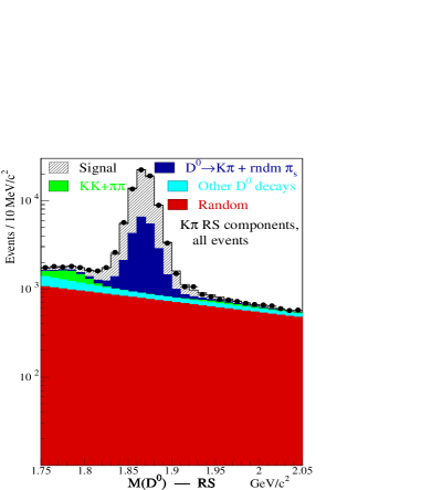
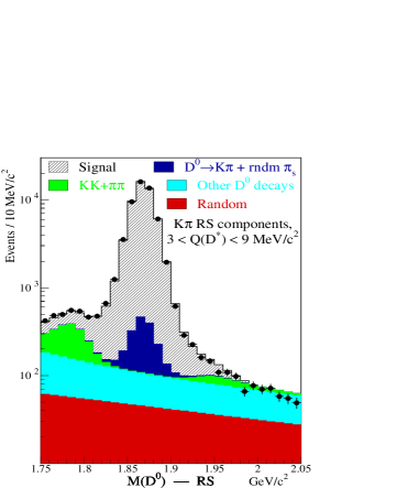
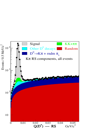
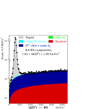
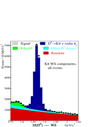
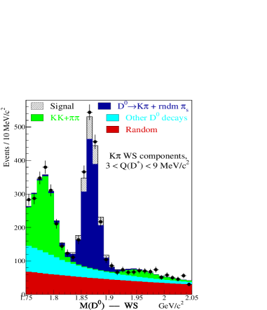
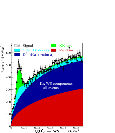
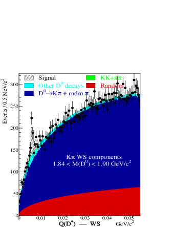
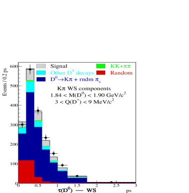
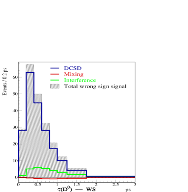
Fits C and C^′ allow for mixing without CP violation (Eq. 1). Representative plots of Fit C are are shown in Figs. 1–3. Figure 1 show the right-sign projections onto $M(D^{0})$ and $Q(D^{*})$, with and without a cut on $Q(D^{*})$ and $M(D^{0})$, respectively. Figure 2 shows the same projections for the wrong-sign events. Figure 3 shows the signal component of the wrong-sign lifetime distribution split into the three components, DCSD, mixing, and interference.

Figure 1: Projection onto $M(D^{0})$ and $Q(D^{*})$ of both the fit (Fit C) and data for right-sign events. The left plots are for all events while the events in the right plots have cuts in the non-plotted variable. Due to the very large signal-to-background, semi-log plots are shown.

Figure 2: Projection onto $M(D^{0})$ and $Q(D^{*})$ of both the fit (Fit C) and data for wrong-sign events. The left plots are for all events while the events in the right plots have cuts in the non-plotted variable.

Figure 3: Projection onto $\tau(D^{0})$ of the fit (Fit C) and data for wrong-sign events. The left plot is for events in the $M(D^{0})$ and $Q(D^{*})$ signal region while the right plot shows the contributions to the wrong-sign signal. The first bin is low due to the necessary inefficiency of vertex separation requirements. The mixing component is negative due to the unphysical value of ${x^{\prime}}^{2}=-0.006$

The DCS branching ratio is found to be $R_{D}=(0.381^{\,+\,0.167}_{\,-\,0.163}\pm 0.092)\%$. The negative log-likelihood is minimized at values of ${x^{\prime}}^{2}=-0.059\%$ and $y^{\prime}=1.0\%$ for Fit C. Due to significant correlations between ${x^{\prime}}$ and $y^{\prime}$ and the fact that ${x^{\prime}}^{2}<0$ is unphysical, the interesting physics result is a contour in the ${x^{\prime}}$, $y^{\prime}$ plane. The minimum negative log-likelihood with ${x^{\prime}}^{2}\geq 0$ occurs at ${x^{\prime}}^{2}=0$ and $y^{\prime}=0.5\%$. Although we fit for ${x^{\prime}}^{2}$, we choose to plot ${x^{\prime}}$. The 95% CL contour is defined as the location in the $x^{\prime}$, $y^{\prime}$ plane where the change in log-likelihood reaches $3.00$ relative to the minimum negative log-likelihood in the physical region of the $x^{\prime}$, $y^{\prime}$ plane. This method has been checked with a frequentist method using mini Monte Carlo with identical results. Systematic checks were performed with 120 fit and cut variants. The contour variation is consistent with differences in the returned value of ${x^{\prime}}^{2}$ and $y^{\prime}$. To assess the systematic uncertainty, we first determine the change in negative log-likelihood between the global minimum and the ${x^{\prime}}$, $y^{\prime}$ location for each of the 120 variants. We then find the value greater than 95% of these differences which is $0.48$. We find the contour at which the change in negative log-likelihood is $3.00+0.48=3.48$ and call this the 95% CL including systematic uncertainties. The contours for Fit C^′ are shown in Fig. 4. We define 95% CL limits on $x^{\prime}$ and $y^{\prime}$ based on the projection of the contour onto the respective axis. The 95% CL limit on $R_{M}$ is defined as the maximum $R_{M}$ value on the contour. The improvement in $-\log{\mathcal{L}}$ compared to Fit A is 0.089 (0.082) for free (restricted) values of ${x^{\prime}}^{2}$.

The last two fits allow for both mixing and CP violation. We do not have sufficient statistics to obtain useful measurements of the mixing and interference CP violating parameters $A_{M}$ and $\sin{\phi}$ (although they are left free in the fit). Thus, the primary results are the DCSD CP violating parameter $A_{D}$ and the mixing parameters. The Fit D and D^′ results come from a fit to the combined $D^{0}$ and $\overline{D}\,\!^{0}$ sample using Eq. 2. The global minimum for Fit D occurs at a highly unphysical ${x^{\prime}}^{2}=-0.52\%$ and $y^{\prime}=6.6\%$ which makes the nominal branching ratio uninteresting. The minimum in the physical plane (Fit D^′) occurs at ${x^{\prime}}^{2}=0.023\%$ and $y^{\prime}=-2.6\%$ with an increase in the log-likelihood fo $0.94$ compared to Fit D. The branching ratio and CP asymmetry for the physical fit are found to be $R_{D}=(0.521^{\,+\,0.144}_{\,-\,0.138}\pm 0.076)\%$ and $A_{D}=0.13^{\,+\,0.33}_{\,-\,0.26}\pm 0.10$. The statistical and statistical+systematic contours are determined in the same manner as in Fit C, as are the 95% CL limits on the mixing parameters. A mini Monte Carlo study using the best fit function to create fake data sets was employed to check the 95% CL contour. Only $92.8\pm 0.8\%$ of the fake data sets had fitted $x^{\prime},y^{\prime}$ values inside the contour. Therefore the contour was increased to include 95% of the fake data sets by increasing $\Delta\log{\mathcal{L}}$ from $3.00$ to $3.50$. The Fit D^′ contours are shown in Fig. 4. The improvement in $-\log{\mathcal{L}}$ of Fit D (D^′) compared to Fit B is 2.51 (1.57).

The last fits, E and E^′, fit the $D^{0}$ and $\overline{D}\,\!^{0}$ samples separately using Eq. 1. From these fits we can calculate $R_{D}=\sqrt{R_{D}^{+}R_{D}^{-}}=(0.518^{\,+\,0.152}_{\,-\,0.145}\pm 0.076)\%$ and $A_{D}=0.12^{\,+\,0.29}_{\,-\,0.28}\pm 0.10$. Contours at the $1-\sqrt{0.05}=77.6\%$ ($\Delta\log{\mathcal{L}}=1.50$) are obtained for each flavor. Every point in the $D^{0}$ contour is combined with every point in the $\overline{D}\,\!^{0}$ contour. The 95% CL $x^{\prime}$, $y^{\prime}$ contour is defined by the outer edge of the resulting points. The systematic error contour is constructed in a fashion similar to Fits C^′ and D^′. The individual $D^{0}$ and $\overline{D}\,\!^{0}$ contours are inflated to $\Delta\log{\mathcal{L}}=1.50+0.12=1.62$ and the combined contour found as before. A mini Monte Carlo study using fake data sets created from the best fit to the data was performed to check the $77.6\%$ CL. The $D^{0}$ $(\overline{D}{}^{0})$ contour was found to encompass significantly less (more) than $77.6\%$ of the fake data sets. Therefore, the contours were each adjusted to include $77.6\%$ of the fake data sets by changing $\Delta\log{\mathcal{L}}$ from the default $1.50$. After this adjustment, the constructed 95% CL limit was found to be consistent with including 95% of the fake data sets. The Fit E^′ contours are shown in Fig. 4. Limits on the mixing parameters are set as in Fits C^′ and D^′ by projecting the contour onto the axes.

Figure 4: 95% CL ${x^{\prime}},{y^{\prime}}$ contours for CP conserving and CP violating fits with ${x^{\prime}}^{2}$ constrained to be greater than zero. The inner curves show the 95% CL contours including statistical uncertainties only while the outer curves also include systematic uncertainties.

6 Conclusions

A compendium of the results from this analysis can be found in Tables 2 and 3. The contours obtained in this analysis [9] agree better with recent results from BABAR [4] and BELLE [10] than with older results from CLEO [11]. The no mixing, no CP violation result agrees with the previous FOCUS result obtained from the same parent data sample but utilizing a very different technique [2]. The two different techniques used to obtain the mixing with CP violation results, Fits $D^{(\prime)}$ and $E^{(\prime)}$, return essentially the same answer. Fit $D^{(\prime)}$ is to be preferred, however, since it retains all correlations in the fit. The results reported here represent the best published charm mixing limit from a fixed-target experiment. In some respects, this measurement is complementary to that obtained from the cleaner, higher statistics $e^{+}e^{-}$ collider experiments. FOCUS has the world’s most accurate lifetime measurements for the six charm species it has measured. In addition, the FOCUS lifetime resolution is far superior to that of the $e^{+}e^{-}$ collider experiments. These strengths, along with significant differences in production and reconstruction, result in a very different analysis from those of the $e^{+}e^{-}$ collider experiments, providing a valuable check on those results.

Table 2: Summary of results for Fits A–D, described in the text.

Measurement	Value	95% CL limit
Fit A: No mixing, CP conserving
$R_{\textrm{WS}}$	$(0.429^{\,+\,0.063}_{\,-\,0.061}\pm 0.027)\%$
Fit B: No mixing, CP violating
$R_{\textrm{WS}}$	$(0.429\pm 0.063\pm 0.028)\%$
$A_{D}$	$0.18\pm 0.14\pm 0.04$	$-0.11<A_{D}<0.48$
Fit C: Mixing, CP conserving, no ${x^{\prime}}^{2}$ constraint
$R_{D}$	$(0.381^{\,+\,0.167}_{\,-\,0.163}\pm 0.092)\%$
${x^{\prime}}^{2}$	$-0.059\%$
$y^{\prime}$	$1.0\%$
Fit C′: Mixing, CP conserving, ${x^{\prime}}^{2}>0$ constraint
$R_{D}$	$(0.395^{\,+\,0.154}_{\,-\,0.098}\pm 0.069)\%$
$R_{M}$		$<0.63\%$
${x^{\prime}}^{2}$	$0.00\%$	$<0.83\%$
$y^{\prime}$	$0.5\%$	$-7.2\%<y^{\prime}<4.1\%$
Fit D: Mixing, CP violating, combined $D^{0}$ and $\overline{D}{}^{0}$ fit, no ${x^{\prime}}^{2}$ constraint
$R_{D}$	$(0.255^{\,+\,0.126}_{\,-\,0.145}\pm 0.132)\%$
$A_{D}$	$0.06^{\,+\,0.46}_{\,-\,0.65}\pm 0.13$
${x^{\prime}}^{2}$	$-0.52\%$
$y^{\prime}$	$6.6\%$
Fit D′: Mixing, CP violating, combined $D^{0}$ and $\overline{D}{}^{0}$ fit, ${x^{\prime}}^{2}>0$ constraint
$R_{D}$	$(0.517^{\,+\,0.147}_{\,-\,0.158}\pm 0.076)\%$
$A_{D}$	$0.13^{\,+\,0.33}_{\,-\,0.25}\pm 0.10$	$-0.42<A_{D}<0.81$
$R_{M}$		$<0.63\%$
${x^{\prime}}^{2}$	$0.023\%$	$<0.80\%$
$y^{\prime}$	$-2.6\%$	$-11.2\%<y^{\prime}<6.7\%$

Table 3: Summary of results for Fit E, described in the text.

Measurement	$D^{0}$ Result	$\overline{D}{}^{0}$ Result
Fit E: Mixing, CP violating, separate $D^{0}$ and $\overline{D}{}^{0}$ fits, no ${x^{\prime}}^{2}$ constraint
$R_{D}^{\pm}$	$(0.275^{\,+\,0.231}_{\,-\,0.233}\pm 0.117)\%$	$(0.458^{\,+\,0.235}_{\,-\,0.226}\pm 0.099)\%$
$R_{D}$	$(0.355^{\,+\,0.175}_{\,-\,0.174}\pm 0.107)\%$
$A_{D}$	$-0.25\pm 0.46\pm 0.14$
${x^{\prime}}^{\pm^{2}}$	$-2.12\%$	$0.61\%$
${y^{\prime}}^{\pm}$	$9.88\%$	$-4.43\%$
Fit E′: Mixing, CP violating, separate $D^{0}$ and $\overline{D}{}^{0}$ fits, ${x^{\prime}}^{2}>0$ constraint
$R_{D}^{\pm}$	$(0.586^{\,+\,0.169}_{\,-\,0.157}\pm 0.079)\%$	$(0.458^{\,+\,0.235}_{\,-\,0.226}\pm 0.099)\%$
$R_{D}$	$(0.518^{\,+\,0.152}_{\,-\,0.145}\pm 0.076)\%$
$A_{D}$	$0.12^{\,+\,0.29}_{\,-\,0.28}\pm 0.10$
$A_{D}$	$-0.46<A_{D}<0.72$ @ 95% CL
$R_{M}$	$<0.61\%$ @ 95% CL
${x^{\prime}}^{\pm^{2}}$	$0.00\%$	$0.61\%$
${y^{\prime}}^{\pm}$	$-1.02\%$	$-4.43\%$
${x^{\prime}}^{2}$	$0.023\%$,     $<0.77\%$ @ 95% CL
$y^{\prime}$	$-2.6\%$,     $-11.0\%<y^{\prime}<6.6\%$ @ 95% CL

7 Acknowledgments

We wish to acknowledge the assistance of the staffs of Fermi National Accelerator Laboratory, the INFN of Italy, and the physics departments of the collaborating institutions. This research was supported in part by the U. S. National Science Foundation, the U. S. Department of Energy, the Italian Istituto Nazionale di Fisica Nucleare and Ministero dell’Istruzione dell’Università e della Ricerca, the Brazilian Conselho Nacional de Desenvolvimento Científico e Tecnológico, CONACyT-México, the Korean Ministry of Education, and the Korean Science and Engineering Foundation.

References

- [1] FOCUS Collaboration, J. M. Link et al., Phys. Lett. B 485 (2000) 62.
- [2] FOCUS Collaboration, J. M. Link et al., Phys. Rev. Lett. 86 (2001) 2955.
- [3] Particle Data Group, S. Eidelman et al., Phys. Lett. B 592 (2004) 1.
- [4] BABAR Collaboration, B. Aubert et al., Phys. Rev. Lett. 91 (2003) 121801.
- [5] FOCUS Collaboration, J. M. Link et al., Nucl. Instrum. and Meth. A 484 (2002) 270.
- [6] FOCUS Collaboration, J. M. Link et al., Nucl. Instrum. and Meth. A 516 (2004) 364.
- [7] F. James and CN/ASD Group, Minuit - Function Minimization and Error Analysis – Reference Manual, Version 94.1, CERN, 1994.
- [8] E. Barbeiro and Z. Was, Comp. Phys. Comm. 79 (1994) 291.
- [9] Contours available at http://www-focus.fnal.gov/kpi_mixing_xycontours.html.
- [10] BELLE Collaboration, J. Li et al., hep-ex/0408125.
- [11] CLEO Collaboration, R. Godang et al., Phys. Rev. Lett. 84 (2000) 5038.