Measurements of Bottom Anti-Bottom Azimuthal Production
Correlations in Proton-Antiproton Collisions at $\sqrt{s}=1.8~{}\rm{TeV}$

Abstract

We have measured the azimuthal angular correlation of $b\overline{b}$ production, using $86.5~{}\rm{pb^{-1}}$ of data collected by Collider Detector at Fermilab (CDF) in $p\overline{p}$ collisions at $\sqrt{s}$=1.8 TeV during 1994$-$1995. In high-energy $p\overline{p}$ collisions, such as at the Tevatron, $b\overline{b}$ production can be schematically categorized into three mechanisms. The leading-order (LO) process is “flavor creation,” where both $b$ and $\overline{b}$ quarks substantially participate in the hard scattering and result in a distinct back-to-back signal in final state. The “flavor excitation” and the “gluon splitting” processes, which appear at next-leading-order (NLO), are known to make a comparable contribution to total $b\overline{b}$ cross section, while providing very different opening angle distributions from the LO process. An azimuthal opening angle between bottom and anti-bottom, $\Delta\phi$, has been used for the correlation measurement to probe the interaction creating $b\overline{b}$ pairs. The $\Delta\phi$ distribution has been obtained from two different methods. One method measures the $\Delta\phi$ between bottom hadrons using events with two reconstructed secondary vertex tags. The other method uses $b\overline{b}\rightarrow(J/\psi X)(\ell X^{\prime})$ events, where the charged lepton ($\ell$) is an electron ($e$) or a muon ($\mu$), to measure $\Delta\phi$ between bottom quarks. The $b\overline{b}$ purity is determined as a function of $\Delta\phi$ by fitting the decay length of the $J/\psi$ and the impact parameter of the $\ell$. Both methods quantify the contribution from higher-order production mechanisms by the fraction of the $b\overline{b}$ pairs produced in the same azimuthal hemisphere, $f_{toward}$. The measured $f_{toward}$ values are consistent with both parton shower Monte Carlo and NLO QCD predictions.

I Introduction

The dominant $b$ quark production mechanism at the Tevatron is believed to be pair production through the strong interaction. However, predictions from next-to-leading order (NLO) perturbative QCD Mangano et al. (1992) have so far failed to describe the observed $b$ single quark production cross section Albajar et al. (1991); Abe et al. (1993a, b, 1995); Acosta et al. (2002); Abachi et al. (1995); Abbott et al. (2000a). Differential cross section measurements have also been systematically higher than theoretical predictions Albajar et al. (1994); Abbott et al. (2000b); Abe et al. (1996, 1997). Possible explanations for the disagreement between the measured and predicted cross sections involve improved $b$ fragmentation models Cacciari and Nason (2002), and non-perturbative $b\overline{b}$ production mechanisms Halzen et al. (1983), and supersymmetric production mechanisms Berger et al. (2001).

Studying $b\overline{b}$ correlations gives additional insight into the effective contributions from higher-order QCD processes to $b$ quark production at the Tevatron. For example, the lowest-order QCD $b\overline{b}$ production diagrams contain only the $b$ and $\overline{b}$ quarks in the final state. Momentum conservation requires that these quarks be produced back-to-back in azimuthal opening angle, $\Delta\phi$, and with balanced momentum transverse to the beam direction, $p_{T}$. However, when higher-order QCD processes are considered, the presence of additional light quarks and gluons in the final state allows the $\Delta\phi$ distribution to become more spread out and the $b$ transverse momenta to become more asymmetric. Previous measurements of azimuthal correlation distributions have yielded varying levels of agreement with NLO predictions Albajar et al. (1994); Abbott et al. (2000b); Abe et al. (1996, 1997); Acosta et al. (2004). Additional measurements related to $b\overline{b}$ production are needed to determine whether experimental measurements are consistent with the Standard Model picture of $b\overline{b}$ production.

The NLO QCD calculation of $b\overline{b}$ production includes diagrams from each production mechanism up to $\mathcal{O}(\alpha_{S}^{3})$. The NLO calculation is the lowest order approach that returns sensible results because certain classes of diagrams which first appear at $\mathcal{O}(\alpha_{S}^{3})$–often referred to as flavor excitation and gluon splitting diagrams (see below)–provide contributions of approximately the same magnitude as the lowest-order diagrams, which are $\mathcal{O}(\alpha_{S}^{2})$. This contribution can be understood by considering the cross section for $gg\to gg$ which is approximately two orders of magnitude larger than the cross section for $gg\to b\overline{b}$. Higher-order $b\overline{b}$ diagrams can be formed from the leading-order diagram $gg\to gg$ by adding a $g\to b\overline{b}$ vertex to either in the initial or final state, but even with the $\mathcal{O}(\alpha_{S})$ suppression, these higher-order diagrams still provide contributions that are numerically comparable to the leading-order terms Mangano et al. (1992); Albajar et al. (1994). Therefore, higher-order corrections to $b\overline{b}$ production cannot be ignored, and a recent measurement indicates that the higher order diagrams contribute a factor of four above the leading order term Acosta et al. (2004).

Figure 1: Example Feynman diagrams that contribute bottom production. The bottom two virtual exchange diagrams enter into the NLO calculation through interferences with leading-order terms. Interferences between the flavor creation, flavor excitation, and gluon splitting diagrams, as well as the virtual exchange diagrams, are ignored in the parton shower approximation

An alternative approach to estimating the effects of higher-order corrections is the parton shower model implemented by the Pythia  Sjostrand and Bengtsson (1987); Bengtsson and Sjostrand (1987) and Herwig Marchesini et al. (1992) Monte Carlo programs. The parton shower approach is not exact to any order in $\alpha_{S}$ but rather tries to approximate corrections to all orders by using leading-order matrix elements for the hard two-to-two QCD scatter and adding addition initial- and final-state radiation using a probabilistic approach. In this approximation, the diagrams for $b\overline{b}$ production can be divided into three categories:

Flavor Creation

refers to the lowest-order, two-to-two QCD $b\overline{b}$ production diagrams. This process includes $b\overline{b}$ production through $q\overline{q}$ annihilation and gluon fusion, plus higher-order corrections to these processes. Because this production is dominated by two-body final states, it tends to yield $b\overline{b}$ pairs that are back-to-back in $\Delta\phi$ and balanced in $p_{T}$.

Flavor Excitation

refers to diagrams in which a $b\overline{b}$ pair from the quark sea of the proton or antiproton is excited into the final state because one of the quarks from the $b\overline{b}$ pair undergoes a hard QCD interaction with a parton from the other beam particle. Because only one of the quarks in the $b\overline{b}$ pair undergoes the hard scatter, this production mechanism tends to produce $b$ quarks with asymmetric $p_{T}$. Often, one of the $b$ quarks will be produced with high rapidity and not be detected in the central region of the detector.

Gluon Splitting

refers to diagrams where the $b\overline{b}$ pair arises from a $g\to b\overline{b}$ splitting in the initial or final state. Neither of the quarks from the $b\overline{b}$ pair participate in the hard QCD scatter. Depending on the experimental range of $b$ quark $p_{T}$ sensitivity, gluon splitting production can yield a $b\overline{b}$ distribution with a peak at small $\Delta\phi$.

Figure 1 illustrates some lowest-order examples of each type of diagram. The general trend is that flavor creation diagrams, being dominated by two-body $b\overline{b}$ final states, tend to produce back-to-back $b\overline{b}$ pairs balanced in $p_{T}$, while flavor excitation and gluon splitting, which necessarily involve multiparticle final states including a $b\overline{b}$ pair and light quarks or gluons, produce $b\overline{b}$ pairs that are more smeared out in $\Delta\phi$ and $p_{T}$. Categorizing $b\overline{b}$ diagrams in this scheme becomes ambiguous at higher order in perturbation theory. In the parton shower approximation, flavor creation, flavor excitation, and gluon splitting processes can be separated exactly based on how many $b$ quarks participate in the hard two-to-two scatter. Interference terms among the three production mechanisms, as well as virtual exchange diagrams, are neglected as higher-order effects in this approximation.

Refs. Field (2002) and Acosta et al. (2004) show that parton shower Monte Carlo programs, which include sizeable contributions from the higher-order $b$ production mechanisms of flavor excitation and gluon splitting, are able to better reproduce the observed $b$ production cross section. Studying $b\overline{b}$ correlations provides a way to tell whether such large contributions from these higher-order processes are supported by the data.

In this paper, we present two new CDF measurements of the $\Delta\phi$ spectrum in $b\overline{b}$ production in $p\overline{p}$ collisions at $\sqrt{s}=1.8~{}\mathrm{TeV}$. These measurements are made using approximately 90 pb^-1 of data collected during the 1994-1995 Tevatron run (known as Run Ib). In addition to providing new information about the entire range of the $b\overline{b}$ $\Delta\phi$ spectrum, these analyses are more sensitive than previous measurements to the low $\Delta\phi$ region, where flavor excitation and gluon splitting make a larger contribution.

One analysis begins with a sample of events containing an 8 GeV electron or muon to enhance the $b$ quark content of the sample by taking advantage of the relatively high semileptonic $B$ branching ratio. These events are then searched for the presence of displaced secondary vertices indicating the decay of a long lived $B$ hadron, using a vertexing algorithm similar to the SECVTX algorithm used for the top quark analyses Abe et al. (1994a); Affolder et al. (2001). This analysis requires that the decay vertices for both $B$ hadrons in the event be reconstructed and extracts the $B$ hadron $\Delta\phi$ distribution from the $\Delta\phi$ distribution measured between the reconstructed secondary vertices. The direction of each $B$ hadron is inferred using the vector sum of the momenta from the secondary vertex tracks and $\Delta\phi$ is defined as the azimuthal angle between the inferred directions of the two $B$ hadrons. This technique yields a high-statistics sample of double-tagged $b\overline{b}$ events and retains sensitivity to $b\overline{b}$ pairs with small opening angles. The second analysis detects the presence of $b$ quark decays in the data entirely through leptonic signatures. The decay of one $b$ is tagged by reconstructing the decay of a $J/\psi\to\mu^{+}\mu^{-}$, which provides the trigger signature that defines this sample. Events are also required to contain an electron or muon consistent with the semileptonic decay of the second $b$. This approach does not yield as many double-tagged events as the first, but it retains the highest sensitivity for $b\overline{b}$ production at small opening angles and has fewer backgrounds. Both analyses produce consistent results indicating that roughly one fourth of the $b\overline{b}$ pairs produced in the momentum and rapidity range to which these analyses are sensitive have $\Delta\phi<90^{\circ}$. In addition, both analyses are at least qualitatively consistent with the contribution from higher order $b\overline{b}$ predicted by Pythia and Herwig, further supporting the significance of the flavor excitation and gluon splitting production mechanisms at the Tevatron.

II Detector

The CDF detector has a cylindrical symmetry about the beam-line, making it convenient to use a cylindrical coordinate system with the $z$-axis along the proton beam direction. We define $r$ to be the distance from the beam-line and $\phi$ to be the azimuthal angle measured from the direction pointing radially outward in the plane of the Tevatron ring. It is also useful to use the polar angle $\theta$ measured with respect to the $z$-axis, and pseudorapidity $\eta=-{\rm ln}\;({\rm tan}\;(\theta/2))$. In the approximation of massless particles, the pseudorapidity equals the rapidity $y=(1/2){\rm ln}\;((E+p_{z})/(E-p_{z}))$, which is the invariant boost of the particle along the $z$-axis. The CDF detector is described in detail elsewhere Abe et al. (1988a). In the following, we focus on the elements most relevant to these analyses.

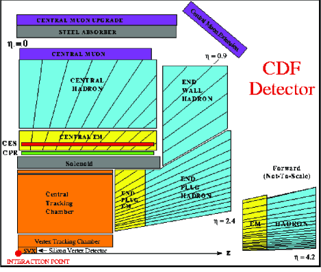
Figure 2: Schematic of a quarter cross-section of the CDF Run 1b detector.

The tracking system, consisting of three different sub-detectors, the central tracking chamber (CTC) Abe et al. (1988b), the vertex detector (VTX), and the silicon vertex detector (SVX^′) Cihangir et al. (1995), is immersed in a uniform 1.4 T solenoidal magnetic field in order to measure the charged particle momentum in a plane transverse to the $z$-axis, denoted as $p_{T}=p\;{\rm sin}\;\theta$. A charged track reconstruction begins with the measurements made in the CTC, which is a large cylindrical multi-wire drift chamber in 3.2 m length along the $z$-axis and centered at the nominal interaction point of the CDF detector. It contains a total of 84 layers of wires positioned between $r=31$ and $133$ cm. The layers are arranged in the alternating groups of 12 with wires parallel to the $z$-axis, known as axial superlayers, and 6 with wires in $\pm 3^{\circ}$ stereo angles, known as stereo superlayers. The VTX, sitting inside the inner radius of the CTC, is a time projection chamber that provides a precise particle trajectory measurement in the $r$$-$$z$ plane and ultimately allows the determination of the $z$-location of the primary interaction point. The innermost system is the SVX^′ covering from $r=2.9$ to $8.1$ cm. This four-layer detector allows high precision determination of particle trajectories in the $r$$-$$\phi$ plane. Combined, the whole tracking system provides a $p_{T}$ resolution of $\delta p_{T}/p_{T}=[(0.0009\times p_{T})^{2}+(0.0066)^{2})]^{1/2}$ and an impact parameter resolution of $\delta d_{0}=[13+(40\;{\rm GeV}/c)/p_{T}]\;\mu\mathrm{m}$.

The central electro-magnetic calorimeter (CEM) Balka et al. (1988), located outside the radius of the CTC and segmented in a projective tower geometry, is designed to be deep enough to contain electro-magnetic showers initiated by electrons or photons. The CEM consists of alternating layers of lead absorber and polystyrene scintillator. A set of wire and strip tracking chambers, known as CES, are embedded in the CEM near the shower maximum or depth of greatest energy deposition, to measure the transverse shower profile. An electron is identified from a track reconstructed in the tracking system that points to an energy deposition in the CEM of appropriate size and matches to a cluster in the CES. For more penetrating particles, the central hadronic calorimeter (CHA) Bertolucci et al. (1988) is located behind the CEM. The CHA is constructed from alternating layers of steel absorber and scintillator, and also segmented in a projective tower geometry. The CHA is used in these analyses primarily to reject hadrons that might fake an electron or a muon signature.

Muons are detected by their ability to penetrate the material in the calorimeter. Three sets of chambers are positioned outside the CHA to identify muons. The first set, known as the central muon (CMU) Ascoli et al. (1988) is located at $r=3.47$ m. A particle traveling perpendicular to the $z$-axis from the primary interaction point must traverse 5.4 pion interaction lengths of material to reach the CMU. An additional set of chambers, the central muon upgrade (CMP) Brandenburg et al. (2002) is arranged in a rectangular array around the CMU behind an additional 60 cm of steel shielding to provide further discriminating power between real muons and hadronic punch-through. To penetrate to the CMP, a particle traveling perpendicular to the $z$-axis from the primary interaction point has to pass through 8.4 pion interaction lengths of material. The CMU and the CMP detectors cover $|\eta|<0.6$. Another set of chambers, the central muon extension (CMX), consisting of four arches of drift chambers located behind 6.2 pion interaction lengths of material, covers $0.6<|\eta|<1.0$. In addition, the CMX drift tubes are sandwiched between two layers of scintillator that provide fast timing information to the trigger. Segments reconstructed from hits in the chambers are known as “stubs”.

The CDF uses a three-level trigger system. The first two levels, named Level-1 and Level-2, are implemented in hardware and reduce the data rate from the full 300 kHz beam crossing rate to a more manageable 20 Hz. The third level, named as Level-3, consists of software algorithms that run a stream-lined version of the full CDF reconstruction software. The triggers used for these analyses rely on lepton identification through matching energy deposition in the CEM (for electron) or muon hits in the CMU, the CMP, and the CMX (for muon) with charged particle tracks reconstructed in the CTC.

III Secondary Vertex Tag $B$ Hadron Correlation Analysis

III.1 Overview

The $\Delta\phi$ distribution of two reconstructed secondary vertex tags has been obtained from data as a probe to investigate the $b\overline{b}$ production mechanisms and compared to the predictions based on Pythia and Herwig Monte Carlo (MC) programs. We correct our data for detector effects and background contributions using MC information in order to extract the $\Delta\phi$ distribution of $B$ hadrons that can be directly compared to the theoretical predictions. We choose to measure the $\Delta\phi$ distribution of $B$ hadrons rather than $b$ quarks, since our secondary vertex tags are more directly related to $B$ hadrons than $b$ quarks. Converting our measurement from the $B$ hadron level to the $b$ quark level would introduce a dependence on $b$ quark fragmentation models that we wish to avoid.

This analysis uses the largest sample of double-tagged $B$ hadron decays ever collected at a hadron collider, extracted from the data taken by CDF during the 1994$-$1995 run of the Tevatron (Run Ib). To create a sample enhanced in $b$ quark content, we take advantage of the high purity of CDF lepton triggers as well as the significant impact parameters of $B$ decay daughters. Each candidate event is required to contain a lepton, either an electron or a muon, presumably coming from the semileptonic decay of one $B$ hadron, and the displaced secondary vertices of both $B$ hadrons. After background removal, we obtain a sample of approximately 17,000 events.

III.2 Secondary Vertex Tagging

Our secondary vertex tagging algorithm looks for tracks consistent with coming from a secondary vertex, significantly displaced from the primary vertex, using the precise tracking information. This algorithm is based on the BVTX algorithm used for the $B^{0}-\overline{B^{0}}$ mixing analysis Abe et al. (1999), which is a modified version of the SECVTX algorithm used for the top quark analysis Abe et al. (1994a); Affolder et al. (2001). The main difference between the version of the BVTX used here and the version used for the previous CDF analyses is the ability to locate more than one secondary vertex per jet searched. For extensive details on the BVTX and the modifications made for this analysis, see Refs. Abe et al. (1999) and  Lannon (2003). Below we summarize the secondary vertex finding approach.

The secondary vertex finding begins by first locating the primary interaction vertex for the event using the precise tracking information. Next the tracks in the event passing quality cuts are grouped into jets using a cone-based clustering algorithm with a cone size of $\Delta R=\sqrt{(\Delta\phi)^{2}+(\Delta\eta)^{2}}=1.0$. Each jet is then searched for the presence of one or more secondary vertices displaced from the primary. Because the secondary vertex finding is done on a jet-by-jet basis, this algorithm is not able to handle the case where the $B$ decay products are contained in more than one jet. However, the relatively large cone-size used in this analysis was chosen to reduce the number of times the a $B$ decay would span more than one jet. The secondary vertex finding is done in two steps for each jet. The first step finds secondary vertices containing at least three tracks. When the first step fails to find any more secondary vertices in a jet, the second step is attempted in which the individual track cuts are made more stringent and two-track secondary vertices are accepted. Each secondary vertex found is required to be significantly displaced from the primary and not to be consistent with the decay of a $K_{S}^{0}$ or $\Lambda$.

III.3 Sample Selection

This analysis starts with the data sample used for the measurement of time dependent $B^{0}-\overline{B^{0}}$ mixing Abe et al. (1999), which is a loosely selected sample that requires each event to have at least an electron or a muon with $p_{T}>8\;{\rm GeV}/c$ identified using the standard CDF lepton identification cuts Lannon (2003), and at least one reconstructed secondary vertex. This sample is known as the BVTX sample, after the name of the secondary vertex tagging algorithm used to create it. The BVTX sample consists of over 480,000 electron-triggered events and over 430,000 muon-triggered events.

The strategy for extracting candidates from the BVTX sample is as follows: Because the BVTX sample was collected with a number of different lepton triggers, we impose specific trigger requirements to ensure the electron and muon subsamples have comparable kinematic properties. Next, the data sample is reprocessed by the modified version of the BVTX algorithm (see section III.2 above) and each event is required to contain at least two secondary vertex tags. The separation $L_{xy}$ between each secondary vertex and the primary vertex in the plane perpendicular to the beam-line divided by the uncertainty on the measurement ($\sigma_{L_{xy}}$) is required to be $L_{xy}/\sigma_{L_{xy}}\geq 2$. To reduce the chance of tagging the same $B$ decay with two poorly measured tags, the 2-dimensional separation between the secondary vertex tags is also required to be $|\Delta L_{xy}|/\sigma_{\Delta L_{xy}}\geq 2$. $\Delta L_{xy}$ is defined to be the distance between the two secondary vertex tags as measured in the plane perpendicular to the beam. Each tag pair is required to have an invariant mass greater than 6 GeV/$c^{2}$ to reduce the chance that a tag pair results from a $B\to D\to X$ decay chain. For a tag pair failing either the $|\Delta L_{xy}|/\sigma_{\Delta L_{xy}}$ or the invariant mass cuts, only the tag with the longest 2-dimensional separation from the primary vertex is removed. Finally, since the trigger requirements for this sample assume at least one of the $B$ hadrons decay semileptonically, the trigger lepton is required to be within a cone of $\Delta R=1.0$ of one of the vertices.

III.4 Sample Composition

We have isolated a high purity $b\overline{b}$ sample in section III.3 with small contamination from other sources. Table 1 shows the sample composition, including background sources that make a contribution to the sample. We briefly summarize each background contribution below.

Scenario	Classification
The tracks in the tag are from the same $B$ decay (including any tracks from a secondary $D$ decay)	Good Tag (Signal)
The tag contains random prompt tracks not associated with the decay of any long-lived particle	Mistag (Background)
The tracks in the tag are from a $B$ decay (including secondary $D$ decay) that has already been tagged with other tracks.	Sequential Double-Tag (Background)
The tag tracks are from a prompt $D$ decay-in other words, a $D$ not associated with the decay of a $B$.	Prompt Charm (Background)

Table 1: Different sources of tags and their classification as signal or background.

A mistag happens when the secondary vertex tagging algorithm tries to fit a vertex from a set of tracks that do not physically originate from a common vertex. Due to errors caused by the tracking performance, it is possible to find a set of prompt tracks that seem to intersect at a vertex displaced from the primary vertex. These vertices distort the correlation spectrum and must be removed. One way to identify mistags is by looking at the distribution of $L_{xy}$, which is signed based on the inferred direction of the particle, namely the direction of the secondary vertex, relative to the primary vertex. A particle that seems to be moving out from the primary vertex at the time of decay obtains a positive $L_{xy}$, while a particle that seems to have been moving towards the primary vertex gets a negative $L_{xy}$. A particle is deemed to be moving away from the primary vertex if the angle between the tag displacement vector (measured from the primary vertex to the secondary vertex tag) and the tag momentum vector is less than 90^∘, and towards the primary vertex otherwise. A secondary vertex corresponding to the decay of real long-lived particle is expected to have a positive $L_{xy}$. However, the finite resolution of the tagging algorithm can yield a negative contribution. As a consequence, mistags make an $L_{xy}$ distribution that is symmetric about zero. We make use of this feature of mistags to subtract them statistically from the data. To understand better how the $L_{xy}$ distribution is used for mistag subtraction, consider the case of an analysis involving only single tags. Half of the total mistag background appears in the negative $L_{xy}$ region. The positive portion of the $L_{xy}$ distribution contains the other half of the mistags, as well as real secondary vertex tags. Therefore, by subtracting twice the number of negative $L_{xy}$ tags from the entire sample of tags, we are left with only the good secondary vertex tags. For analyses such as this one, which considers pairs of secondary vertex tags, the calculation is given by

$$N_{GG}=N_{++}-N_{+-}-N_{-+}+N_{--},$$ (1)

where $N_{GG}$ is the estimated number of tag pairs in which both tags are legitimate secondary vertex tags, while $N_{++}$ is the number of tag pairs in which both tags have $L_{xy}>0$, $N_{+-}$ and $N_{-+}$ are the number of tag pairs in which one tag has a positive $L_{xy}$ and the other has a negative $L_{xy}$, and $N_{--}$ is the number of tag pairs in which both tags have $L_{xy}<0$. Conceptually, in this equation, we are using the second and third terms to subtract mistags from the tag pairs represented by the first term. However, $N_{+-}$ and $N_{-+}$ each contain a contribution from the case where both tags are mistags and by subtracting them both, this contribution is double-counted. The last term in the equation corrects this. To obtain a mistag subtracted distribution, Eq. 1 is applied on a bin-by-bin basis.

Another possible source of background involves tagging more than one secondary vertex from a single $B$ decay. These tags, known as sequential tags, are most likely to occur when the $B$ decay involves the production of a $D$ hadron that travels a certain distance from the $B$ decay vertex before itself decaying. The invariant mass cut of 6 GeV/$c^{2}$ eliminates virtually all contribution from this source. Although this cut does reduce the tagging efficiency at low opening angle, it is necessary to keep the sequential tag background from overwhelming the signal in that region. This efficiency reduction is accounted for in the Monte Carlo modeling of the data. It is also possible that some sequential tag pairs arise from tracking errors that cause tracks originating from a common vertex to be reconstructed as coming from two vertices that are very close together. The cut on the significance of the 2-dimensional separation between the tags ($|\Delta L_{xy}|/\sigma_{\Delta L_{xy}}$) eliminates nearly all these tag pairs. The residual contribution from sequential double tags is estimated in section III.7.

Finally, a background source of legitimate secondary vertices is direct $c\overline{c}$ production. In general, most $D$ hadrons have a much smaller lifetime than $B$ hadrons. However, those $D$ hadrons that do live long enough to produce a secondary vertex capable of being tagged by BVTX will not be removed or accounted for by any of the methods mentioned above. In addition, it is possible to have events in which multiple heavy flavor pairs, such as $b\overline{b}+c\overline{c}$ and $b\overline{b}+b\overline{b}$, are produced. For example, in a flavor creation event, an additional $c\overline{c}$ pair may be produced through gluon splitting. In such events it is possible for the $b\overline{b}$ to contribute one tag and the $c\overline{c}$ to contribute another. Although the rate of multiple heavy flavor production is much lower than single $b\overline{b}$ production, the opportunity to tag more displaced vertices in a given event can provide an enhancement in tagging acceptance, meaning such processes cannot be discounted outright. Our MC studies indicate that the combined contribution to the tag pair sample from prompt charm and multiple heavy flavor production is not large, roughly 10%. The subtraction of this contribution and the associated systematic error are described in section III.7.

III.5 Monte Carlo Samples

The parton shower MC programs, Pythia Sjostrand and Bengtsson (1987) and Herwig Marchesini et al. (1992), are used to generate large samples of $b\overline{b}$ events. Because flavor creation, flavor excitation, and gluon splitting mechanisms do not interfere with each other in the parton shower model, each mechanism is generated separately. For Pythia, the flavor creation samples are generated as the heavy flavor production process using massive matrix elements for $q\overline{q}\to b\overline{b}$ and $gg\to b\overline{b}$ diagrams. Flavor excitation and gluon splitting samples are produced as the generic QCD 2-to-2 process using massless matrix elements, and then separated from other QCD processes by examining the partons that participate in the 2-to-2 hard scattering. Three Pythia samples with different amounts of initial state radiation (ISR) are generated for each mechanism: The samples are dubbed low, medium, and high ISR, as explained in appendix A. The choice to investigate different ISR settings in Pythia is motivated primarily because the ISR tuning of Pythia was changed in the recent past based on studies of heavy flavor production Norrbin and Sjostrand (1998, 2000), and the new tuning produces a noticeably different $\Delta\phi$ spectrum from the previous version. The low ISR sample corresponds to the most recent ISR settings in Pythia while the high ISR sample reflects the previous default settings. In principal, changes in the amount of final state radiation (FSR) would have a similar affect, but such an effect has not been studied here. For all three Pythia samples, the underlying event is tuned to match observations in CDF data Field . On the other hand, because there are fewer parameters to tune, only one Herwig sample is generated for each mechanism. The Herwig flavor creation and flavor excitation samples are generated with heavy flavor production option including massive matrix element treatments of the LO flavor creation and flavor excitation diagrams. As in Pythia, the Herwig gluon splitting component results from generating all QCD 2-to-2 processes using massless matrix elements and retaining those events classified as gluon splitting based on the partons involved in the hard scattering. In addition, a small sample of $c\overline{c}$ events was generated using Pythia, for the purpose of evaluating the possible effects of residual prompt charm as a background for this analysis. Both Pythia and Herwig generation used the CTEQ5L parton distribution functions. See Appendix A for more information about the Pythia and Herwig parameters used for this analysis. For all samples, heavy flavor decays are handled by the CLEO QQ MC program Avery et al. (1985). Finally, to make the MC data resemble the actual data as closely as possible, the MC events are passed through a CDF detector simulation, a CDF trigger simulation, and the same reconstruction and analysis code used for the actual data. Additional details regarding the generation of MC samples can be found in Ref. Lannon (2003).

III.6 Data–Monte Carlo Comparison

After the Monte Carlo samples have been passed through the detector simulation as described above, the Monte Carlo predictions for the secondary vertex tag distributions can be compared directly with data. Distributions involving individual tags have similar shapes for flavor creation, flavor excitation, and gluon splitting, and so these distributions can be used to check whether the detector simulation adequately models detector effects. Distributions involving tag pairs, and therefore correlations, give information about how well the Monte Carlo models describe $b\overline{b}$ production.

Figure 3 shows the comparison of the trigger electron $p_{T}$ and $E_{T}$ and the trigger muon $p_{T}$ between the data and each Monte Carlo sample. Figure 4 shows the comparison of the secondary vertex tag properties in the Monte Carlo and data. In each case, the agreement between the measured spectrum from the data and the predicted spectra for each Monte Carlo sample indicates that the effects of trigger and reconstruction thresholds are adequately modeled in the simulation. In addition, examining the Monte Carlo truth information for the $B$ hadrons tagged by the analysis code allows a determination of the effective minimum $B$ $p_{T}$ sensitivity for this analysis. For the $B$ producing the 8 GeV/c trigger lepton, this measurement is sensitive only to $B$ hadrons with a minimum $p_{T}$ of 14 GeV/c, while the requirement that the other $B$ be tagged by the BVTX algorithm sets a minimum $p_{T}$ acceptance of 7.5 GeV/c $p_{T}$.

Figure 3: The trigger electron $p_{T}$ and $E_{T}$ and the trigger muon $p_{T}$ distributions from data compared to the high ISR Pythia Monte Carlo sample. The comparisons of data to other Monte Carlo samples is similar and can be found in Ref. Lannon (2003). The muon trigger threshold is clearly visible in the lower plot. The small number of muons below the 8 GeV trigger threshold come from events containing a second muon that passes the offline selection.

Figure 4: The secondary vertex tag distributions from electron data compared to the high ISR Pythia Monte Carlo sample. Comparisons involving muon data and comparisons to other Monte Carlo samples are similar and can be found in Ref. Lannon (2003).

Comparing tag pair correlations between the Monte Carlo samples and the data reveals whether Pythia or Herwig provide an adequate model of the higher-order contributions to $b\overline{b}$ production. This analysis focuses on the transverse opening angle, $\Delta\phi$. For tag pairs, $\Delta\phi$ is defined as the angle between the $p_{T}$ vectors determined by taking the vector sum of the $p_{T}$ from all the tracks involved in the tag. The $\Delta\phi$ distribution is interesting to study because it is sensitive to contributions from flavor excitation and gluon splitting. Also, the broadness of the back-to-back peak in $\Delta\phi$ is sensitive to the amount of initial-state radiation present in the Monte Carlo. It should be noted that the shape of the $\Delta\phi$ distribution and the relative contributions from the three production mechanisms depend on the $p_{T}$ cuts placed on each of the $B$ hadrons.

There are two possible approaches to normalizing the relative contributions in Monte Carlo from flavor creation, flavor excitation, and gluon splitting. Pythia and Herwig each provide predictions for the cross section of each production mechanism, and these cross sections can be used to normalize their contributions relative to one another. Alternatively, one could take the position that Pythia and Herwig may not correctly model the amount of each contribution, and the relative contributions should be determined to provide the best match to data. In this analysis, both approaches are examined. As described in the sections below, the data is compared to the Monte Carlo predictions in two ways. First, the Monte Carlo prediction for the cross section of each production mechanism is used to normalize the flavor excitation and gluon splitting components relative to the flavor creation contribution. In this “fixed normalization” scheme, the data is compared to the Monte Carlo using one arbitrary global normalization parameter. The arbitrary global normalization is included because this analysis attempts only a shape comparison, not an absolute cross section measurement. In addition, the Monte Carlo and data are compared using a “floating normalization” scheme. In this comparison, each production mechanism is given an independent arbitrary normalization constant and the three normalizations are varied to yield the best match to data.

Figure 5 shows the comparison of the BVTX tag $\Delta\phi$ distribution from data to the distribution predicted by each Monte Carlo sample when the relative normalization of each production mechanism is based on the Monte Carlo prediction for the cross sections of the different production mechanisms. From these $\Delta\phi$ comparisons it can be seen that each Monte Carlo model matches the qualitative features of the data, although there are definite differences in shape, as reflected by the poor $\chi^{2}$ values. For the Pythia sample with low initial-state radiation (ISR), the peak in the back-to-back region is too narrow, while for the medium and high ISR samples, the back-to-back peak is too broad. Similarly, the Herwig Monte Carlo sample also has a peak that is too broad at high $\Delta\phi$, perhaps even more so than in Pythia. However, aside from these discrepancies at high $\Delta\phi$, the rest of the $\Delta\phi$ distribution matches reasonably well between Monte Carlo and data using the normalizations predicted by the Monte Carlo generators for the different production mechanisms. The $\chi^{2}$ values between the $\Delta\phi$ curves from Monte Carlo and data are listed in Table 2. On the basis of these $\chi^{2}$ values, it appears that Pythia with the medium ISR value provides the best match to data when using the Monte Carlo s default normalization for the three production mechanisms. Figure 6 shows the breakdown of the contributions from the individual production mechanisms to the overall $\Delta\phi$ shape for this Pythia sample.

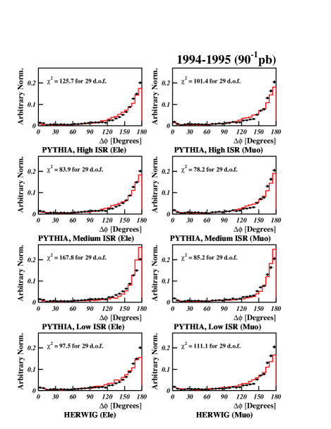
Figure 5: Comparisons between the shape of the tag $\Delta\phi$ distribution for data (points) and the tag $\Delta\phi$ distribution predicted by the various Monte Carlo samples (line). The contributions from flavor creation, flavor excitation and gluon splitting are added together according to the individual Monte Carlo cross section predictions for these contributions and only a single common normalization is varied to get the best match to data. The $\chi^{2}$ values shown in the plots account only for the data and Monte Carlo statistical errors.

Figure 6: A detailed comparison between the $\Delta\phi$ distribution from data (points, statistical errors only) and the $\Delta\phi$ distribution from Pythia with medium ISR (solid line). In addition, the contributions from flavor creation (dashes), flavor excitation (dots), and gluon splitting (dash-dots) are shown. The contributions are normalized according to Pythia’s cross section predictions and an arbitrary global normalization is used to give the best shape fit between data and Monte Carlo.

Note that mistag subtraction applied to the individual Pythia contributions can result in negative values for bins with few entries. Consequently, the total Pythia distribution can be less than one of the components in some bins.

However, since, in the parton shower approximation, the contributions from flavor creation, flavor excitation, and gluon splitting may be generated separately, each component can have a separate, arbitrary normalization and the three components can be fit for the combination of normalizations that gives the best match to the shape of the $\Delta\phi$ spectrum from data. These fits are shown in Figure 7. When the normalizations of the individual components are allowed to float with respect to one another, one can obtain rather good agreement in shape between data and both the low ISR and high ISR Pythia samples. The fit of the low ISR Pythia Monte Carlo to the data increases the broader contribution from flavor excitation to compensate for the narrowness of the back-to-back peak from flavor creation. For the high ISR Pythia samples, the peak at high $\Delta\phi$ is made narrower to match the data by all but eliminating the contribution from flavor excitation. A comparison of the relative fractions of each production mechanism in the two Pythia fits is shown in Figure 8. The fit of the Herwig sample to the data also tries to compensate for the excessive broadness of the Herwig flavor creation peak at high $\Delta\phi$, but even after completely eliminating the flavor excitation contribution, the remaining contribution from flavor creation at high $\Delta\phi$ is too broad to model the data. Table 2 compares the fit quality and effective contribution from flavor creation, flavor excitation, and gluon splitting in the fits of the various Monte Carlo samples to the data. Both low ISR and high ISR Pythia samples can be made to fit the data with approximately the same fit quality, which is unexpected, especially since the low ISR sample accomplishes this fit with a high flavor excitation content while the high ISR sample fits with almost no flavor excitation contribution. In the end, there seems to be an ambiguity in Pythia that allows a trade-off between initial state-radiation and the amount of flavor excitation.

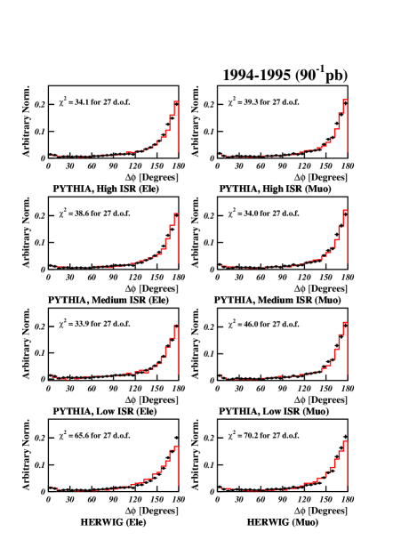
Figure 7: Comparisons between the shape of the tag $\Delta\phi$ distribution for data (points) and the tag $\Delta\phi$ distribution predicted by the various Monte Carlo samples (line). In these comparisons, the normalizations of each production mechanism were allowed to vary independently and were chosen to give the best fit between the Monte Carlo and the data. Again, the fit $\chi^{2}$ takes into account Monte Carlo statistics in addition to errors on the data.

Figure 8: A comparison of the contributions from flavor creation (dashes), flavor excitation (dots), and gluon splitting (dash-dots) to the total $\Delta\phi$ shapes (solid) for Pythia with high ISR (top) and low ISR (bottom). Electron Monte Carlo is shown in the plots. The muon plots can be found in Ref. Lannon (2003). The normalization of each component is set by the best fit of the three components to the spectrum from data. Note that mistag subtraction applied to the individual Pythia contributions can result in negative values for bins with few entries. Consequently, the total Pythia distribution can be less than one of the components in some bins.

	Electrons				Muons
	Fixed Normalization		Floating Normalization		Fixed Normalization		Floating Normalization
Pythia	FC:	$43.7\%$	FC:	$66.1\%$	FC:	$41.4\%$	FC:	$64.5\%$
High ISR	FE:	$40.7\%$	FE:	$1.7\%$	FE:	$41.5\%$	FE:	$8.1\%$
	GS:	$15.6\%$	GS:	$32.2\%$	GS:	$17.1\%$	GS:	$27.4\%$
$\chi^{2}/d.o.f.$	125.7/29		34.1/27		101.4/29		39.3/27
$\chi^{2}$ probability	$5.26\times 10^{-14}$		0.136		$5.83\times 10^{-10}$		0.0595
Pythia	FC:	$47.7\%$	FC:	$65.3\%$	FC:	$46.5\%$	FC:	$63.2\%$
Medium ISR	FE:	$35.8\%$	FE:	$0.2\%$	FE:	$35.3\%$	FE:	$8.6\%$
	GS:	$16.5\%$	GS:	$34.5\%$	GS:	$18.2\%$	GS:	$28.2\%$
$\chi^{2}/d.o.f.$	83.9/29		38.6/27		78.2/29		34.0/27
$\chi^{2}$ probability	$3.07\times 10^{-7}$		0.0688		$4.11\times 10^{-6}$		0.166
Pythia	FC:	$68.3\%$	FC:	$37.6\%$	FC:	$63.9\%$	FC:	$48.5\%$
Low ISR	FE:	$12.0\%$	FE:	$51.4\%$	FE:	$13.9\%$	FE:	$34.6\%$
	GS:	$19.7\%$	GS:	$11.0\%$	GS:	$22.2\%$	GS:	$16.9\%$
$\chi^{2}/d.o.f.$	167.8/29		33.9/27		85.2/29		46.0/27
$\chi^{2}$ probability	$1.76\times 10^{-21}$		0.169		$1.96\times 10^{-7}$		0.0127
Herwig	FC:	$57.6\%$	FC:	$70.9\%$	FC:	$55.7\%$	FC:	$74.8\%$
	FE:	$24.0\%$	FE:	$0.0\%$	FE:	$23.1\%$	FE:	$0.0\%$
	GS:	$18.4\%$	GS:	$29.1\%$	GS:	$21.2\%$	GS:	$25.2\%$
$\chi^{2}/d.o.f.$	97.5/29		65.6/27		111.1/29		70.2/27
$\chi^{2}$ probability	$2.45\times 10^{-9}$		$4.65\times 10^{-5}$		$1.52\times 10^{-11}$		$1.05\times 10^{-5}$

Table 2: Comparison of the effective contributions from flavor creation (FC), flavor excitation (FE), and gluon splitting (GS) to fits of the Monte Carlo $\Delta\phi$ to the data. The fit $\chi^{2}$ takes into account Monte Carlo statistics in addition to errors on the data. The “$\chi^{2}$ probability” entry refers to the probability of getting a worse fit, according to the $\chi^{2}$ distribution.

In general, any of the Monte Carlo samples compared to the data shows reasonable qualitative agreement. The Monte Carlo sample that best matches the data is Pythia with medium or high ISR settings, when the individual normalizations of the flavor creation, flavor excitation, and gluon splitting are allowed to float separately to best fit the data. Although the fit using Pythia with low ISR is not so poor as to rule this model out completely, studies indicate that Pythia with high initial state radiation does a better job of matching both the underlying event and minimum bias data at CDF Field . Therefore, we select the Pythia sample, with high ISR and the relative normalizations of flavor creation, flavor excitation, and gluon splitting fixed by our fit to the $\Delta\phi$ distribution of the data, as the best Monte Carlo model of the data. Comparisons indicate that the differences between Pythia with medium or high ISR settings are minor. Figure 9 shows a comparison of other correlations between the data and Pythia with high ISR. Although these plots show good agreement between the data and Pythia for the overall shapes of the distributions, the shapes of the individual contributions from flavor creation, flavor excitation, and gluon splitting are not distinct enough to allow a separation of the components as was done for the $\Delta\phi$ distribution.

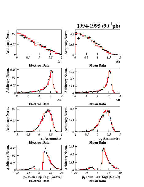
Figure 9: A comparison of Pythia with high ISR to the data for several different correlation quantities. The normalizations for the three production mechanisms in Pythia have been determined by the fit of the Pythia $\Delta\phi$ distributions to data. The $p_{T}$ asymmetry is given by $A_{p_{T}}=(p_{T}(lep)-p_{T}(non-lep)/(p_{T}(lep)+p_{T}(non-lep)$ . In the $p_{T}(Non-LepTag)$ plot, the sign of the $p_{T}$ is determined by the opening angle between the lepton-tag and the non-lepton tag: negative for tag pairs with $\Delta\phi<90^{\circ}$, positive otherwise. The data are shown as points with statistical error bars only. The solid line is Pythia with high ISR

It is interesting to note that before allowing the normalizations of each production mechanism to float in the fits, the agreement between Herwig and the data is no worse than the agreement between the low ISR Pythia sample and the data. However, because the disparity between the data and the low ISR Pythia sample comes from the narrowness in the flavor creation peak at high $\Delta\phi$, when the normalizations are allowed to float, the fit can alleviate the disagreement by increasing the peak width through a higher contribution from flavor excitation. In contrast, for Herwig, once the contribution from flavor excitation has been reduced to zero, the fit has no way to make the width of the back-to-back flavor creation peak smaller, short of the unphysical situation of setting the flavor excitation normalization negative. If there were some other parameter for Herwig, like Pythia s initial state radiation parameter, PARP(67), that could be used to tune the width of the back-to-back flavor creation peak, it may be possible to achieve good agreement between Herwig and the data as well.

The results presented here can be compared to another analysis of lepton tags in heavy-flavor events presented in Ref. Acosta et al. (2004). That analysis compares Herwig to double-tagged events using higher $E_{T}$ jet samples. In addition to using a sample of double-tagged events at higher momentum, Ref. Acosta et al. (2004) also differs from this analysis in that it uses calorimeter based jets as opposed to the tracking jets utilized here, and the quantity measured is the azimuthal opening angle between the tagged jets rather than the angle between the tags themselves. In agreement with this analysis, that one clearly shows the importance of the higher-order contributions in heavy flavor production, and also shows an agreement with Herwig that is better than the agreement seen in this analysis. Perhaps this suggests that the disagreement shown here between Herwig and the data is related to Herwig s ability to model low $p_{T}$ $b$ production or $b$ fragmentation.

III.7 Corrections and Systematics

The correlations examined so far in the data involve pairs of BVTX tags, rather than pairs of $B$ hadrons. There are detector effects, such as the tagging efficiency for pairs of $B$ hadrons as a function of $\Delta\phi$, that distort the shape of the measured tag pair correlations from the true $B$ hadron distribution. In addition, residual contributions from background can affect the shape of the tag pair distribution. For the comparison between MC and data, the detector effects are accounted for by using a detector and trigger simulation to adjust the MC to match the conditions in the data, while the backgrounds are assumed to be negligible. However, since the MC models examined in section III.6 match the data reasonably well, MC events can be used to determine the relationship between the measured tag pair distribution and the actual $B$ hadron distribution. In the sections below, two kinds of corrections to the tag pair $\Delta\phi$ distribution are considered: a correction for the relative tagging efficiency, which is a detector effect, and a correction for the contributions from mistags, prompt charm, and sequential decays that remain in the data after the steps taken in section III.4 to remove backgrounds. In addition, the MC is used to estimate the systematic uncertainties associated with correcting for the relative tagging efficiency and removing background events. These corrections and systematic errors are evaluated using several different MC samples to account for uncertainties involved in the MC model itself.

The BVTX tagging algorithm is not equally effective for all topologies of $b\overline{b}$ production. In particular, it becomes more difficult for the BVTX algorithm to reconstruct both displaced secondary vertices as the opening angle between the two $B$ hadrons decreases. This effect becomes especially severe when the two $B$ hadrons are both contained within the cone of a single jet for track clustering purposes. Furthermore, correlations between opening angle and $p_{T}(B)$ for the various production mechanisms can lead to differences in the relative efficiency for reconstructing tag pairs at different opening angles. These effects distort the shape of the $\Delta\phi$ distribution measured for tags from the true $B\overline{B}$ $\Delta\phi$ distribution.

We correct for these relative efficiency effects using the MC that best matches the data, as determined in section III.6. Because we are only examining the shape of the $\Delta\phi$ distribution, our goal in making this correction is only to account for differences in the relative efficiency of the tagging algorithm, as a function of $\Delta\phi$. We do not attempt to correct for effects that impact all parts of the $\Delta\phi$ spectrum equally. For example, an overall shift in the muon trigger efficiency would not affect this correction. To determine the correction for each bin we take the ratio of the number of tag pairs reconstructed in the MC to the number of pairs that could have been reconstructed if the tagging algorithm had perfect efficiency. The number of tag pairs that would have been reconstructed assuming perfect efficiency is determined by looking at the generator level $B$ hadron $\Delta\phi$ distribution. For electron MC, to simulate the electron trigger, we require one $B$ hadron in the event to have a $p_{T}>14.0\;{\rm GeV}/c$ and $|\eta|<1.0$. For the muon MC, we demand one $B$ hadron with $p_{T}>14.0\;{\rm GeV}/c$ and $|\eta|<0.6$. For both cases, we require a second $B$ hadron with $p_{T}>7.5\;{\rm GeV}/c$ and $|\eta|<1.0$. The cuts placed on the generator-level MC were determined by examining the $p_{T}$ and $\eta$ distributions for $B$ hadrons from MC events in which two BVTX tags were reconstructed. The $p_{T}$ and $\eta$ values were chosen by determining the cuts for which 90% of the $B$ hadrons in the double-tagged MC events would pass. We take the $\Delta\phi$ distribution resulting from the event selection above and convolute it with a Gaussian resolution function with a width of 0.1086 radians, characteristic of the $\Delta\phi$ resolution of the BVTX tagging algorithm as measured in MC.

In order to minimize the effect of statistical fluctuations in the tagging efficiency determined from MC, we fit the tagging efficiency to an empirical function of the following form:

$$\epsilon(\Delta\phi) = P_{1}\exp\left\{-\frac{1}{2}\left(\frac{\Delta\phi^{2}}{P_{2}^{2}}\right)\right\}+$$ (2)

$$P_{3}\exp\left\{-\frac{1}{2}\left[\frac{(\Delta\phi-\pi)^{2}}{P_{4}^{2}}\right]\right\}+$$

$$P_{5}\mathrm{freq}\left(\frac{\Delta\phi-P_{6}}{P_{7}}\right)+P_{8}(\Delta\phi)+P_{9},$$

where $\mathrm{freq}$ is the error function. The relative efficiency curve resulting from this fit is shown in Fig. 10. The sharp step around $\phi=60^{\circ}$, which is modeled by the error function term, comes from the transition from the case of finding secondary vertex tags in two separate jets to finding secondary vertex tags in the same jet. Since we are only interested in the effect of the efficiency on the shape of the $\Delta\phi$ distribution, and not on its absolute normalization, we have rescaled the curve in Fig. 10 so that the relative efficiency in the last $\Delta\phi$ bin is defined to be unity. Thus this curve shows the effect of the BVTX tagging efficiency for a given bin relative to the last $\Delta\phi$ bin.

Figure 10: The bin-by-bin values for the relative efficiency returned by the fit. The curves have been normalized so that the last $\Delta\phi$ bin has a value of one by definition. The error bars on these curves indicate the statistical error on the bin values returned from the fit. The statistical errors for the fit are correlated from bin to bin.

There are two main contributions to the systematic uncertainty associated with the relative tagging efficiency correction. First, the statistical errors on the fit value for the relative efficiency correction factor should be propagated into systematic uncertainties on the corrected $\Delta\phi$ distribution. There is an additional systematic uncertainty that comes from the model used to calculate the relative efficiency correction. The Pythia MC sample, with high ISR and with the normalization of the different production mechanisms taken from the fit to the $\Delta\phi$ distribution in the data, is used as our baseline for the relative efficiency correction. However, other models, like the lower ISR Pythia sample or Herwig also match the data to varying degrees and so could also have been used. To account for this ambiguity, we compare the relative efficiency corrections from other MC models to our baseline model. In the worst case, the difference for the bin-by-bin relative efficiency correction factor is approximately equal in magnitude to the statistical error from the fit. Therefore, to account to modeling uncertainties in the relative efficiency correction, we increase the systematic error associated with the correction by a factor of $\sqrt{2}$ .

The mistag subtraction scheme used for this analysis relies on the assumption that 100% of legitimate tags and 50% of mistags have positive $L_{xy}$. The true fraction may be somewhat different. For example, if most of the events contain at least one $B$ hadron, then the $L_{xy}$ distribution of mistags may be biased towards positive values by the presence of actual displaced tracks in the events. Furthermore, the bias in $L_{xy}$ may depend on the topology of the event. To investigate any possible bias in the $L_{xy}$ distribution of mistags, we examined MC events containing mistags identified by matching tracking information to MC truth information. From MC sample to MC sample, the fraction of legitimate secondary vertex tags that have positive $L_{xy}$ varies from 0.97 to 1.0. For mistags, the positive $L_{xy}$ fraction varies from 0.45 to 0.55. To estimate the possible effect of using the wrong fractions when performing mistag subtraction, we redo the mistag subtraction in the data using different assumptions about the positive $L_{xy}$ fraction for good tags and mistags. The mistag subtraction formula (Eq. 1), generalized for an arbitrary fraction $p$ of good tags with positive $L_{xy}$ and an arbitrary fraction $q$ of mistags with positive $L_{xy}$, is given by

$$N_{GG}=\frac{(q-1)^{2}}{(q-p)^{2}}N_{++}+\frac{q(q-1)}{(q-p)^{2}}N_{+-}$$

$$+\frac{q^{2}}{(q-p)^{2}}N_{--}+\frac{q(q-1)}{(q-p)^{2}}N_{-+}$$ (3)

Changing the positive $L_{xy}$ fractions from mistag subtraction affects both the normalization and the shape of the $\Delta\phi$ distribution. However, we are only concerned about the shape for this analysis. Therefore, before we compare the shape of the $\Delta\phi$ distribution using the standard mistag subtraction scheme to the shape obtained using alternative values for the positive $L_{xy}$ fractions, we normalize the distributions to unit area. To estimate the systematic error from mistag subtraction, we take the $\Delta\phi$ distributions calculated varying the $p$ and $q$ values in Eq. 3 within their allowed ranges and fit them to the functional form for the $\Delta\phi$ distribution, given below, in order to minimize the effect of statistical fluctuations:

$$f(\Delta\phi) = P_{1}\exp\Big{[}-\frac{1}{2}\Big{(}\frac{\Delta\phi}{P_{2}}\Big{)}^{2}\Big{]}+$$ (4)

$$P_{3}\exp\Big{[}P_{4}(\Delta\phi-\pi)^{2}+P_{5}(\Delta\phi)\Big{]}+$$

$$P_{6}\Delta\phi+P_{7}$$

We then calculate the maximum deviation between the result from the default mistag subtraction scheme and the results obtained from varying the positive $L_{xy}$ fractions. This maximum deviation is assigned as the systematic error on the $\Delta\phi$ shape from mistag subtraction.

The bin-by-bin contribution to the double-tag $\Delta\phi$ distribution from prompt charm is estimated primarily using MC. The overall amounts of prompt charm and $b\overline{b}+c\overline{c}$ double tags are estimated by comparing the relative rate of obtaining a double-tagged $b\overline{b}$ MC event to the rates for double-tagging $c\overline{c}$ and $b\overline{b}+c\overline{c}$ MC events. This approach estimates that 2.9% (6.0%) of the tag pairs in this sample come from $c\overline{c}$ production for electron (muon) data, and 1.8% of the tag pairs in both the electron and the muon samples comes from $b\overline{b}+c\overline{c}$ production. The $\Delta\phi$ shape for the $c\overline{c}$ and $b\overline{b}+c\overline{c}$ contributions is estimated by applying the measured relative tagging efficiency as a function of $\Delta\phi$ to the generator level $c\overline{c}$ and $b\overline{b}+c\overline{c}$ $\Delta\phi$ distributions. The resulting estimated contamination from prompt charm to the double-tag $\Delta\phi$ distribution is shown in Fig. 11. The systematic error on this correction is estimated by performing several checks on the data. One check involves comparing the $\Delta\phi$ spectrum for double-tagged events in which the invariant mass of the tracks for each tag is greater than 2 GeV/$c^{2}$ to the spectrum when both tags have an invariant mass less than 2 GeV/$c^{2}$. The former sample is enhanced in $b\overline{b}$ content relative to prompt charm, while the latter sample has a greater contribution from prompt charm. Both subsamples have far fewer statistics than the main sample. The $\Delta\phi$ shapes of these two subsamples agree within the statistics of the samples, suggesting a negligible contribution from prompt charm. An alternative estimation of the prompt charm contribution can be obtained by fitting the tag mass distribution to template shapes derived from $b\overline{b}$ events (including tags of secondary charmed mesons) and $c\overline{c}$ events. The results of these fits suggest a prompt charm contamination roughly a factor of two larger than the MC estimates, although still a relatively small contribution at 7.1% for the electron data and 13.3% for the muon data. As a result of the differences between these two alternate estimates of the prompt charm contribution and the MC method used to set the normalization of our prompt charm correction, we set the systematic error on the prompt charm correction equal to the size of the correction in each bin.

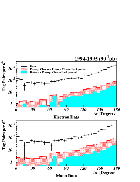
Figure 11: The estimated shape of the background from direct $c\overline{c}$ production (the hatched area) and multiple-heavy flavor ($b\overline{b}+b\overline{b}$ and $b\overline{b}+c\overline{c}$) production (the solid area). The points with error bars show the data.

The MC is also used to determine the residual contribution from sequential double tags. Based on examining MC events in which two tags are identified to come from the same $B$ decay, we determine that after mistag subtraction, 25.9% of the tags removed by the 6 GeV/$c^{2}$ mass cut were from sequential tag pairs. Furthermore, using Monte Carlo it was also determined that for every 100 mistags removed by the 6 GeV/c² mass cut, roughly 2.41 events remained in this sample, yielding an efficiency for this cut of 97.6%. In the data, after mistag subtraction, the 6 GeV/$c^{2}$ invariant mass cut removes 471 tags from the electron sample and 598 tags from the muon sample. Using the numbers derived from the MC above, this means that of the tags removed by the invariant mass cut, 122.1 electron and 155.0 muon tags come from sequential double tag pairs, and an estimated 2.9 electron sequential tag pairs and 3.7 muon sequential tag pairs remain in the data after this cut. The $\Delta\phi$ distribution of the sequential tag pairs is also determined using MC to be well described by the positive half of a Gaussian distribution with a mean of zero and a width of 0.122 radians. To correct for the sequential double tag contribution in the data, we take the estimated number of sequential double tags, with a half-Gaussian distribution as described above, and subtract them from the $\Delta\phi$ bins in the data. The systematic error on this correction is set equal to the size of the correction.

III.8 Final Distribution and Comments

Figure 12 shows the final, corrected tag $\Delta\phi$ distribution, including systematic errors. To obtain this distribution, the contributions from residual sequentials and prompt charm are removed from the mistag-subtracted distributions. Then the relative efficiency corrections derived in Section III.7 are applied. Systematic errors from the various corrections are combined in quadrature to give the total systematic error. Mistag subtraction gives the largest contribution to the systematic error. The final corrected tag $\Delta\phi$ distribution provides a measurement of the $B-\overline{B}$ $\Delta\phi$ distribution where the $B$ providing the trigger electron (muon) has $p_{T}>14.0$ GeV/c and $|\eta|<1.0(0.6)$, and the other $B$ has $p_{T}>7.5$ GeV/c and $|\eta|<1.0$, with a $\Delta\phi$ resolution of $6.22^{\circ}$. This distribution can be compared to generator-level $\Delta\phi$ distributions from Monte Carlo that have been convoluted with a Gaussian resolution function to account for our $\Delta\phi$ resolution. Finally, ignoring the small difference in $\eta$ acceptance between the electron and muon samples, these two distributions can be combined to give the overall $B$ hadron $\Delta\phi$ distribution, shown in Figure 13. Table 3 specifies the corrected fraction in each $\Delta\phi$ bin as well as the breakdown of the systematic errors for each bin.

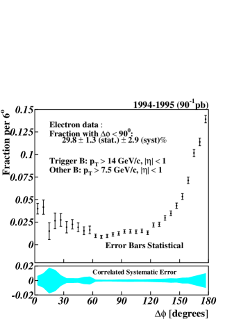
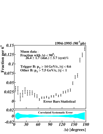
Figure 12: The final, corrected $\Delta\phi$ distribution for the double-tagged electron (left) and muon (right) data. The corrections made to the data include mistag subtraction, sequential removal, prompt charm subtraction, and the relative tagging efficiency correction. The error bars display the statistical error on the points. The filled region at the bottom indicates the systematic errors. The systematic errors are correlated from bin to bin. Mistag subtraction provides the dominant contribution to the systematic errors.

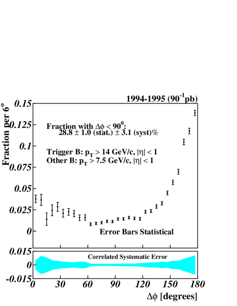
Figure 13: The combined, corrected electron and muon $\Delta\phi$ distribution from the double-tagged analysis. In making this plot, we ignored the difference in $\eta$ acceptance between the electron and muon triggers. The corrections made to the data include mistag subtraction, sequential removal, prompt charm subtraction, and the relative tagging efficiency correction. The error bars display the statistical error on the points. The filled region at the bottom indicates the systematic errors. The systematic errors are correlated from bin to bin. Mistag subtraction provides the dominant contribution to the systematic errors.

				Systematic Error Components
Bin	Fraction	Statistical Error	Systematic Error	Sequential	Prompt Charm	Mistag Subtraction	Relative Efficiency
$0^{\circ}-6^{\circ}$	0.03901	0.00462	0.00593	0.00060	0.00051	0.00421	0.00411
$6^{\circ}-12^{\circ}$	0.03765	0.00684	0.01042	0.00044	0.00082	0.00982	0.00336
$12^{\circ}-18^{\circ}$	0.01347	0.00774	0.00833	0.00013	0.00125	0.00810	0.00149
$18^{\circ}-24^{\circ}$	0.02498	0.00674	0.00544	0	0.00084	0.00472	0.00257
$24^{\circ}-30^{\circ}$	0.02942	0.00561	0.00472	0	0.00087	0.00370	0.00279
$30^{\circ}-36^{\circ}$	0.02152	0.00493	0.00372	0	0.00074	0.00309	0.00194
$36^{\circ}-42^{\circ}$	0.02323	0.00420	0.00336	0	0.00069	0.00256	0.00206
$42^{\circ}-48^{\circ}$	0.02077	0.00379	0.00298	0	0.00101	0.00211	0.00185
$48^{\circ}-54^{\circ}$	0.01568	0.00349	0.00472	0	0.00093	0.00171	0.00380
$54^{\circ}-60^{\circ}$	0.01651	0.00344	0.00461	0	0.00043	0.00137	0.00438
$60^{\circ}-66^{\circ}$	0.00751	0.00167	0.00114	0	0.00087	0.00054	0.00049
$66^{\circ}-72^{\circ}$	0.00869	0.00151	0.00102	0	0.00084	0.00037	0.00044
$72^{\circ}-78^{\circ}$	0.00973	0.00153	0.00090	0	0.00073	0.00030	0.00045
$78^{\circ}-84^{\circ}$	0.01156	0.00156	0.00079	0	0.00059	0.00025	0.00047
$84^{\circ}-90^{\circ}$	0.01100	0.00155	0.00097	0	0.00085	0.00022	0.00040
$90^{\circ}-96^{\circ}$	0.01423	0.00157	0.00130	0	0.00084	0.00023	0.00046
$96^{\circ}-102^{\circ}$	0.01395	0.00160	0.00128	0	0.00121	0.00026	0.00040
$102^{\circ}-108^{\circ}$	0.01559	0.00162	0.00120	0	0.00117	0.00033	0.00040
$108^{\circ}-114^{\circ}$	0.01474	0.00163	0.00172	0	0.00106	0.00044	0.00034
$114^{\circ}-120^{\circ}$	0.01370	0.00177	0.00212	0	0.00159	0.00057	0.00029
$120^{\circ}-126^{\circ}$	0.02203	0.00187	0.00259	0	0.00195	0.00071	0.00045
$126^{\circ}-132^{\circ}$	0.02244	0.00193	0.00268	0	0.00242	0.00082	0.00045
$132^{\circ}-138^{\circ}$	0.02813	0.00213	0.00344	0	0.00246	0.00088	0.00059
$138^{\circ}-144^{\circ}$	0.03128	0.00223	0.00303	0	0.00328	0.00080	0.00069
$144^{\circ}-150^{\circ}$	0.04471	0.00249	0.00465	0	0.00279	0.00051	0.00106
$150^{\circ}-156^{\circ}$	0.05622	0.00275	0.00466	0	0.00444	0.00018	0.00137
$156^{\circ}-162^{\circ}$	0.06983	0.00306	0.00716	0	0.00419	0.00113	0.00169
$162^{\circ}-168^{\circ}$	0.10516	0.00341	0.00914	0	0.00583	0.00267	0.00319
$168^{\circ}-174^{\circ}$	0.11783	0.00346	0.01105	0	0.00688	0.00457	0.00391
$174^{\circ}-180^{\circ}$	0.13944	0.00336	0.00419	0	0.00779	0.00662	0.00419

Table 3: The corrected fraction of combined electron and muon data in each bin as well as a breakdown of the components of the systematic errors on each bin. The total systematic error is the sum in quadrature of the individual components.

From the corrected data, we can also calculate the fraction of tag pairs in the “towards” region, defined by $\Delta\phi<90^{\circ}$ . This fraction is of interest because $\Delta\phi$ production in the “towards” region is dominated by the higher order production diagrams. The towards fraction provides a single figure of merit to indicate the relative sizes of the contributions from flavor excitation and gluon splitting. To account for correlated systematic errors, we calculate the towards fraction for our data by essentially repeating the analysis with two $\Delta\phi$ bins instead of thirty, and then taking the ratio of the “towards” bin over the total. For the electron data, we obtain a towards fraction of $29.8\pm 1.3(stat.)\pm 2.9(syst.)\%$. For muon data, we obtain a towards fraction of $26.4\pm 1.7(stat.)\pm 3.7(syst.)\%$. The electron and muon samples are combined to give a towards fraction of $28.8\pm 1.0(stat)\pm 3.1(syst)\%$. Table 4 shows the uncorrected number of tag pairs in the “towards” and “away” bins in the data and gives the corrections applied to obtain the final number. Table 5 breaks down the contributions to the systematic uncertainty on the towards fraction.

	Electrons		Muons
	Towards	Away	Towards	Away
Mistag-Subtracted Data	1210	8887	832	6260
Charm Contamination	42.1	442.6	52.9	500.3
Sequential Contamination	2.9	0.0	3.7	0.0
Relative Efficiency Correction Factor	0.326	1.0	0.376	1.0
Corrected Data	3573.6	8444.4	2062.2	5759.7

Table 4: The number of events in the “towards” and “away” regions before and after applying corrections to the data.

	Electrons	Muons
Towards Fraction	29.8%	26.4%
Statistical Error	$\pm 1.3\%$	$\pm 1.7\%$
Mistag Subtraction Systematic Error	$\pm 2.0\%$	$\pm 2.8\%$
Sequential Removal Systematic Error	$\pm 0.05\%$	$\pm 0.09\%$
Charm Subtraction Systematic Error	$\pm 1.3\%$	$\pm 2.2\%$
Relative Efficiency Correction Systematic Error	$\pm 1.6\%$	$\pm 1.1\%$
Total Systematic Error	$\pm 2.9\%$	$\pm 3.7\%$

Table 5: The break-down of the systematic errors by contribution. The total systematic error is the quadrature sum of the individual components.

IV ${\boldmath J/\psi}$–lepton ${\boldmath b}$ Quark Correlation Measurement

IV.1 Overview

This measurement is optimized to measure the region in phase space least understood in experimental measurements and theoretical predictions: small $\Delta\phi$ where both bottom quarks point in the same azimuthal direction. As stated previously, earlier bottom quark angular production measurements had little sensitivity to this region. A study of opposite side flavor tags using soft leptons for the CDF $\sin{2\beta}$ measurement Affolder et al. (2000a) showed a significant number of tags at small opening angles between fully reconstructed bottom decays and the soft leptons. Figure 14 shows the sideband-subtracted $\Delta\phi$ distribution between $B^{+}\rightarrow J/\psi K^{+}$ candidates and the soft leptons. About $30\%$ of the soft leptons are in the same azimuthal hemisphere, a fraction much larger than expected from parton shower flavor creation Monte Carlo ($\approx 5\%$ for Pythia flavor creation).

Figure 14: Sideband-subtracted $\Delta\phi$ distribution between fully reconstructed $B^{+}\rightarrow J/\psi K^{+}$ and soft leptons.

This analysis uses the bottom pair decay signature of $b\rightarrow J/\psi X,\overline{b}\rightarrow\ell^{+}X$. The impact parameter of the additional lepton and the pseudo-$c\tau$ of the $J/\psi$ are fit simultaneously in order to determine the $b\overline{b}$ fraction of the two $\Delta\phi$ regions. Angular requirements that were necessary in previous di-lepton measurements because of double sequential semi-leptonic decay backgrounds($b\rightarrow c\ell^{-}X;c\rightarrow\ell^{+}X^{\prime}$) are avoided by the chosen signal. $B_{c}$ is the only particle that decays directly into $J/\psi$ and an addition lepton. The only other source of candidates where the additional lepton and $J/\psi$ candidates originate from the same displaced decay are hadrons that fake leptons or decay-in-flight of kaons and pions. The number of events from $B_{c}$ or from ‘fake’ leptons can be estimated well by using techniques from Ref. Abe et al. (1998a). Thus, no angle requirement between the two candidate bottom decay products are necessary, yielding uniform efficiency over the entire $\Delta\phi^{b\overline{b}}$ range. Due to the limited size of the data sample, only $f_{toward}$, the fraction of $b\overline{b}$ pairs in the same azimuthal hemisphere, can be measured.

The selection criteria used in this analysis have similar bottom momenta and rapidity acceptances to CDF’s Run II displaced track(SVT) Bardi et al. (2002) and $J/\psi$ triggers, and the addition leptons have momenta very similar to the opposite side taggers planned for Run II (opposite kaon, opposite lepton and jet charge flavor taggers). Therefore, this measurement aids in the development and understanding of flavor taggers for such Run II measurements as the $B_{s}$ mass difference.

IV.2 Sample Selection

The signal searched for in this analysis is $b\rightarrow J/\psi X,\overline{b}\rightarrow\ell^{+}X^{\prime}$ where $\ell$ can be an electron or muon. In this section, the Run IB $J/\psi$ data set is described. The offline selection criteria for both the $J/\psi$ and the additional lepton are also described.

IV.2.1 $J/\psi\rightarrow\mu^{+}\mu^{-}$ Selection

This analysis uses the CDF Run Ib $J/\psi$ data set obtained between January 1994 and July 1995. The CDF $J/\psi$ triggers and offline $J/\psi$ selection criteria utilized are the same as the $B_{c}$ discovery analysis at CDF Abe et al. (1998a). In order to understand the trigger efficiencies, we confirm that the $J/\psi$ candidate’s muons are the two muon candidates which triggered the event.

After confirming the trigger, the position of the extrapolated track at the muon chamber is compared to the position of the muon stub using a $\chi^{2}$ matching test, taking into account the effects of multiple scattering and energy loss in material. The positions are required to match within 3 standard deviations in the r–$\phi$ projection and within 3.5 standard deviations in the r–z projection.

Next, we require a high quality track for both muon candidates. The pseudo-lifetime ($c\tau$) of the $J/\psi$ candidates is used in this analysis to determine the bottom purity. Therefore, SVX^′ information is required in order to improve the precision of the $c\tau$ measurement.

In order to reject $J/\psi$ candidates with muons originating from different primary interactions, the z position difference between the two tracks is required to be less than 5 cm at the beam-line. A vertex constrained fit of the two muon candidates is performed Marriner (1993). The $\chi^{2}$ probability of the vertex fit is required to be better than $1\%$. The vertex constrained mass of the $J/\psi$ candidate is required to be $2.9~{}{\rm GeV}<{\rm M}_{J/\psi}<3.3~{}{\rm GeV}$.

A total of 177,650 events pass the above selection cuts. Figure 15 shows the $J/\psi$ mass distribution for these events. In order to estimate the number of $J/\psi\rightarrow\mu^{+}\mu-$ candidates, the mass has been fit with two Gaussians (used to model the $J/\psi$ signal) and a linear background term. A linear background has been assumed in many previous CDF $J/\psi$ analyses Abe et al. (1998a, b); Affolder et al. (2000b). The background under the mass peak is caused by irreducible decay-in-flight and punch-though backgrounds, Drell-Yan muons and double sequential semi-leptonic decays where $b\rightarrow c\mu^{-}X,c\rightarrow s\mu^{+}X^{\prime}$. From the fit, $137780\pm 440$ $J/\psi$ candidates are in the sample. For this measurement, the $J/\psi$ mass signal region is defined to be within $\pm 50~{}\rm{MeV}$ of the Particle Data Group Groom et al. (2000) world average value (3096.87 MeV). The sideband regions are chosen to be $2.900~{}\rm{GeV}\leq M_{J/\psi}\leq 3.000~{}\rm{GeV}$ and $3.200~{}\rm{GeV}\leq M_{J/\psi}\leq 3.300~{}\rm{GeV}$. The sideband regions contain 20,180 events. The events in these regions are used later in the analysis to describe the $c\tau$ shape of $J/\psi$ background in the mass signal region.

Figure 15: Di-muon invariant mass distribution from events passing selection criteria. Top: Linear scale. Bottom: Logarithmic scale.

The ratio between the number of background $J/\psi$ events in the mass signal region to the background in the mass sideband region ($R_{side}$) was determined to be $R_{side}=0.501\pm 0.000043$ by the mass fit. To estimate the systematic uncertainty of this ratio, a 2nd order polynomial is used to describe the background term. The resulting fit value is $R_{side}=0.545\pm 0.008$. The difference between the two fits is taken to be the systematic uncertainty yielding $R_{side}=0.501\pm 0.044.$

IV.2.2 CMUP $\mu$ Selection Requirements

The additional (non-$J/\psi$) muon is required to have muon stubs in both the CMU and CMP (a CMUP muon). Requiring both CMU and CMP muon stubs maximizes the amount of material traversed by the candidate, reducing the background due to hadronic punch-though of the calorimeter. The $\chi^{2}$ matching requirements are the same as for the $J/\psi$ muons. The muon candidates are required to have a $p_{T}>3~{}\rm{GeV}$; muons with lower $p_{T}$ will typically range out prior to the CMP due to energy loss in the calorimeter and the CMP steel.

As the impact parameter is used to estimate the bottom purity of the muons, the same track quality is required as for the $J/\psi$ muons. Additionally, the muon candidate’s track projection is required to be in the fiducial volume of the CMU and CMP. The z positions of the $J/\psi$ candidate and the CMUP muon are required to be within 5 cm of each other at the beam-line.

In total, 247 CMUP candidate muons are found in the $J/\psi$ sample, out of which 51(142) CMUP candidates are in events where the $J/\psi$ candidate is in the mass sideband (signal) region.

Of the 142 CMUP candidates with $J/\psi$ candidates in the $J/\psi$ mass signal region, 64 events have the CMUP muon and the $J/\psi$ candidate in the same hemisphere in the azimuthal angle (which will be known as toward); the other 78 events have the CMUP muon and $J/\psi$ candidate in the opposite hemisphere in the azimuthal angle (which is denoted away).

IV.2.3 Electron Selection Criteria

A method of the finding soft (relatively low momenta) electrons was developed for bottom flavoring tagging in CDF’s $B_{d}$ mixing and $sin(2\beta)$ measurements Abe et al. (1999); Affolder et al. (2000a). These electrons have a relatively high purity, a transverse momenta greater than 2 GeV, and an understood efficiency. The rate of hadrons faking an electron was studied extensively in Ref. Abe et al. (1998a), making it possible to estimate the background due to hadrons faking electrons. The selection criteria is identical to Ref. Abe et al. (1998a) in order to use the same fake rate estimates.

The selection criteria requires a high quality track which is consistent with an electron in the various detector systems. Information on the energy (charge) deposited, the cluster location, and track matching $\chi^{2}$ variables are all used in order to reduce the rate of a hadron in the detectors’ fiducial volume faking an electron to $\left(6.4\pm 0.6\right)\times 10^{-4}$.

One source of electron background is photon conversions, where a photon interacts with detector material and converts into a $e^{+}e^{-}$ pair. In addition, $1.2\%$ of all neutral pions decay into $\gamma e^{+}e^{-}$ directly (Dalitz decay). To reduce this background, conversions are searched for and vetoed by looking for a conversion partner track.

The conversion requirements are the same as Ref. Abe et al. (1999). Unfortunately, the conversion removal is not totally efficient. Therefore, some of the soft electron candidates are residual conversion electrons, where either the conversion pair track is not found due to tracking inefficiencies at low $p_{T}$ or the conversion electron selection is not fully efficient. The rate of residual conversions is studied more in section IV.3.4.

In total, 514 candidate electrons are found after conversion removal; 92 events have the $J/\psi$ candidate in the mass sidebands and 312 events have the $J/\psi$ candidate in the mass signal region. In the $J/\psi$ mass signal region, 107(205) of the events are in the toward(away) regions in $\Delta\phi$. In the $J/\psi$ mass signal region, 6(9) events were vetoed as conversions in the toward(away) $\Delta\phi$ bin. In the $J/\psi$ mass sideband region, 5(4) events were vetoed as conversions.

IV.3 Signal and Background Description

The signal and backgrounds for both the $J/\psi+\mu$ and $J/\psi+e$ samples are very similar. The basic technique to determine the amounts of the various signal and background components is with a simultaneous fit of the pseudo-$c\tau$ (defined in section IV.3.1) of the $J/\psi$ and the signed impact parameter of the non-$J/\psi$ lepton. The impact parameter is signed to distinguish between residual electron conversions and electrons from bottom decay, as described in section IV.3.5. The impact parameter is signed positive if the primary vertex lies outside the r–$\phi$ projection of the particle’s helix fit.

As the $J/\psi$ and additional lepton originate from separate bottom hadron decays, the impact parameter of the additional lepton and the $c\tau$ of the $J/\psi$ are not strongly correlated for the signal. The backgrounds in this analysis have two categories: one in which the impact parameter and $c\tau$ are uncorrelated, and other where the impact parameter and $c\tau$ are strongly correlated. The impact parameter and the $c\tau$ become strongly correlated when both the $J/\psi$ and the additional lepton candidate originate from the same displaced vertex.

In uncorrelated sources, the impact parameter and $c\tau$ shapes describing the background are determined independently. $J/\psi$ candidates are assumed to originate from three sources: direct $J/\psi$ production (including feed-down from $\chi_{c1}$, $\chi_{c2}$, and $\psi(2s)$) where the $J/\psi$ decays at the primary vertex, $J/\psi$ from bottom decay (including the feed-down from higher $c\overline{c}$ resonances), and the non-$J/\psi$ background described by the events in the $J/\psi$ mass sidebands. Lepton candidates are assumed to originate from the following sources: directly produced fake or real leptons from the primary vertex, leptons from bottom decay (including $b\rightarrow cX\rightarrow\ell X^{\prime}$), lepton candidates with the fake $J/\psi$ candidate, and residual conversion electrons.

In addition, two correlated sources of backgrounds exist. The first source is $B_{c}\rightarrow J/\psi\ell^{+}X$, which is a small but irreducible background. The impact parameter of the additional lepton and the $c\tau$ of the $J/\psi$ is described by Monte Carlo techniques and the overall size of the background is also estimated (see section IV.3.7).

The other correlated source of background occurs when a bottom hadron decays into a $J/\psi$ and a hadron which is misidentified as a lepton. For electrons, this background is due to hadrons (mostly $\pi^{\pm}$ and $K^{\pm}$) showering early in the calorimeter and passing the electron identification selection. For muons, there are two sources of this background. The largest source of correlated background is due to decay-in-flight of charged pions and kaons, which result in a real muon. These real muons are denoted as ‘fakes’ in this analysis. The other, smaller correlated fake muon background is caused by hadrons punching through the calorimeter and muon steel shielding. These background sources are more fully described in section IV.3.8.

The following sections provide a description of the techniques used to determine the impact parameter and $c\tau$ shapes of the various sources and to estimate of the number of residual conversions, $B_{c}\rightarrow J/\psi\ell X$ events, and $b\rightarrow J/\psi\ell_{\rm{fake}}X$ events in the sample.

IV.3.1 $J/\psi$ $c\tau$ Signal and Background Distributions

The direct $J/\psi$ and bottom decay $J/\psi~{}c\tau$ shapes are determined from a fit to the data, using a technique previously establish in Ref. Abe et al. (1998b); Affolder et al. (2000b). The relatively long average lifetime of the bottom hadron ($1.564\pm 0.014~{}\rm{ps}$ Groom et al. (2000)) allows one to distinguish between these two sources. First, the signed transverse decay length $L_{xy}$ is determined in the r–$\phi$ plane.

$$L_{xy}\equiv\frac{\left(\vec{X}_{SV}-\vec{X}_{PV}\right)\cdot\vec{p}_{T}^{~{}J/\psi}}{p_{T}^{J/\psi}},$$ (5)

where $\vec{X}_{SV}$ and $\vec{X}_{PV}$ are the locations of the $J/\psi$ vertex and the primary vertex in the transverse plane, and $\vec{p}_{T}^{~{}J/\psi}$ is the vector transverse momentum of the $J/\psi$. Directly produced $J/\psi$ have a symmetric $L_{xy}$ distribution around zero and bottom $J/\psi$ events will predominately have a positive sign. If the bottom decay was fully reconstructed, one could determine the proper decay length exactly ($c\tau_{proper}$) from the measured $L_{xy}$ and $p_{T}$. Because the bottom hadron is not fully reconstructed, a ‘pseudo-proper decay length’ ($c\tau$) is constructed using the kinematics of the $J/\psi$ only:

$$c\tau\equiv\frac{L_{xy}\cdot m_{J/\psi}}{p_{T}^{J/\psi}\cdot F_{corr}(p_{T}^{J/\psi})}.$$ (6)

$F_{corr}(p_{T}^{J/\psi})$, determined in Ref. Abe et al. (1998b), is the average correction factor for the partial reconstruction of the bottom hadron.

The events in the $J/\psi$ mass sidebands are used to model the fake $J/\psi$ background under the $J/\psi$ mass signal peak. Two components are fit using an unbinned log-likelihood technique: events from the primary vertex (direct) and events with lifetime from heavy flavor (predominantly from $b\rightarrow c\mu^{-}X\rightarrow\mu^{+}X^{\prime}$). The direct events are described by a symmetric resolution function chosen to be a Gaussian plus two symmetric exponentials. The events with lifetime are fit with a positive only exponential.

Once the $c\tau$ shape of the mass sideband events is found, the $c\tau$ shapes of directly produced and bottom decay $J/\psi$ can be determined. The shape of the directly produced $J/\psi$ ($F_{direct}^{c\tau}(x)$) is parameterized by a Gaussian with two symmetric exponential tails; this shape is the assumed resolution function of the $c\tau$ measurement. The shape of $J/\psi$ events from bottom decay ($F_{b}^{c\tau}(x)$) is therefore described as a positive exponential convoluted with the $c\tau$ resolution function. The background shape ($g_{back}$) is fixed to the value obtained in the fit of the sideband region and the background fraction ($f_{back}$) is fixed to the value predicted by the $J/\psi$ candidate mass fit. Figure 16 shows the fit result of the signal region. The fit average bottom proper decay length of $442\pm 5~{}\mu\rm{m}$ is consistent with previous measurements at the Tevatron Abe et al. (1998b); Affolder et al. (2000b). The fit yields a bottom fraction of $16.6\%\pm 0.2\%$ or equivalently $22150\pm 270$ $J/\psi$ from bottom decay.

Figure 16: Fit of $J/\psi$ signal region.

IV.3.2 Lepton Impact Parameter Signal Distributions

The impact parameter shape of bottom decay leptons is determined by Monte Carlo simulation, using the prescription from Ref. Field (2002) for parton shower Monte Carlo programs. In this prescription, separate samples of flavor creation, flavor excitation, and gluon splitting events are generated and then combined with the relative rates predicted by the Monte Carlo programs. In appendix B, the generation of the simulated events is described.

Figure 17 shows the unsigned impact parameter for direct bottom electrons ($b\rightarrow ce^{-}$) and sequential charm electrons ($b\rightarrow c\rightarrow se^{+}$) in the flavor creation sample. The impact parameter distributions are very similar and cannot be fit for separately. The uncertainty on the relative rate of these two sources is one of the systematic uncertainties treated in section IV.4.1. The bottom decay impact parameter shape is fit with two symmetric exponentials and a Gaussian. The fit to the simulated bottom impact parameter distribution for electrons is shown in fig. 18.

Figure 17: The impact parameter of events with electrons passing requirement in the flavor creation Monte Carlo sample. Top: Direct bottom. Bottom: Sequential charm.

Figure 18: The signed impact parameter distribution for the combined electron bottom Monte Carlo. Top: Logarithmic scale. Bottom: Linear scale.

IV.3.3 Lepton Impact Parameter Background Distributions

In previous analyses Abe et al. (1996, 1997), the impact parameter distributions for particles originating at the primary vertex were determined using jet data. Unfortunately, any data sample will have low level contamination of heavy flavor (charm or bottom) at the $\approx 0.1-1\%$ level, which is larger than the non-Gaussian effects in the impact parameter resolution. In this analysis, the impact parameter shapes of directly produced particles are determined with a Monte Carlo technique.

Pythia is used to generate the light quark and gluon subprocesses, which are then passed through a detector simulation. To be included in the electron sample, the candidates must be a quality track with a $p_{T}>2~{}\rm{GeV}$ and extrapolate into the electron fiducial region. For the muon direct sample, the candidates must have a quality track with a $p_{T}>3~{}\rm{GeV}$ and extrapolate into the CMUP muon fiducial region. The simulation events which pass the selection criteria are fit with two symmetric exponentials and a Gaussian. The fit shapes are then used as input to the likelihood fit for particles originating from the primary vertex (direct tracks).

IV.3.4 Size of Residual Conversion Background

One obvious source of electron background is residual conversions left in the sample due to the inefficiency of finding the conversion pair. In order to estimate the number of residual conversions, a technique similar to Ref. Long (1998) is used. It is assumed that there are two independent causes for the lack of removal of a conversion electron: the track pair is lost due to tracking inefficiencies at low momenta or the selection requirements are not fully efficient. By measuring these two efficiencies and the rate of conversion removal with the chosen conversion selection requirements, one determines the residual electrons ($N_{resid}$). The conversion electron that passes the electron identification criteria is denoted as the conversion candidate, and other electron that did not pass the electron identification criteria is denoted as the pair candidate.

The number of residual electrons is equal to:

$$N_{resid}=N_{tag}\cdot\left(\frac{1}{\epsilon_{cnv}(cut)}\cdot\frac{1}{\epsilon_{cnv}(p_{T})}-1\right)$$ (7)

where $N_{tag}$ is the number of the conversions removed, $\epsilon_{cnv}(cut)$ is the conversion finding efficiency, and $\epsilon_{cnv}(p_{T})$ is the tracking efficiency of the conversion pair.

The efficiency $\epsilon_{cnv}(cut)$ is measured using different sets of conversion requirements, the tight (standard) and a loose set of cuts. Assuming that the loose cuts are fully efficient, the ratio of conversion pairs fit with tight and loose cuts yields $\epsilon_{cnv}(cut)=72.3\pm 6.5\%$. In order to test this assumption, 2 additional wider sets of cuts are used which yield no extra conversion candidates.

The tracking efficiency of the pair candidates ($\epsilon_{cnv}(p_{T})$) is estimated with a Monte Carlo technique similar to Ref. Abe et al. (1998a). The generation of the simulated conversions is detailed in Appendix B. $\epsilon_{cnv}(p_{T})$ is estimated by comparing the $p_{T}$ distribution of the conversion partner in the simulation sample to the $p_{T}$ distribution of the conversion partners in the data sample. The simulation is normalized to the data in the $p_{T}$ range where the tracking is fully efficient ($p_{T}>0.5~{}\rm{GeV}$). The ratio of the number of events seen in data versus the number of normalized conversion candidates in simulation gives $\epsilon_{cnv}(p_{T})=69\pm 5(\rm{stat})\pm 9(\rm{syst})\%$. The systematic error includes the uncertainty in the conversion’s $p_{T}$ spectra.

The ratio of the number of residual to found conversions was found to be $R_{conv}=1.00\pm 0.38$. The conversion veto removes 6(9) electron candidates in the toward(away) $\Delta\phi$ region. Thus, approximately 6.0 (9.0) residual conversion are in toward(away) $\Delta\phi$ region. About $5\%$ of the electron candidates are residual conversions and have to be included in the $c\tau$–impact parameter fit. A total of 9 conversions (4 toward, 5 away) are found in events with the $J/\psi$ candidate in the mass sideband region.

IV.3.5 Impact Parameter Shape of Residual Conversion Background

For conversion electrons from a primary photon, the primary vertex alway lies outside of the helix projection with perfect tracking. To distinguish between conversions and bottom decay electrons, the impact parameter is signed such that the impact parameter is positive if the primary vertex is outside the r-$\phi$ projection of the track’s helix and is negative otherwise. Conversion electrons are positively signed, and Dalitz decay electrons and bottom decay electrons are equally negatively and positively signed.

The vast majority of the conversion candidates are signed positive as predicted (shown in fig. 19). Unfortunately, there is a large positive tail which is not consistent with the number of silicon hits assigned to the track. Since at least 3 SVX^′ hits are required, one would expect the conversion candidates either to originate from the first two silicon layers or the beam pipe, or to be a $\pi^{0}$ Dalitz decay from the primary vertex. These sources would produce conversions with a impact parameter less than 0.04 cm. Therefore, a fraction of the conversion candidates must have mis-assigned silicon hits and originate outside of the SVX^′. The measured conversion radius for 25 of the 62 conversion candidates is greater than 6 cm, which is outside of the second silicon layer.

To construct an impact parameter shape for residual conversions, two Monte Carlo samples are generated: a sample in which the silicons hits are correctly assigned (low conversion radius, $R_{conv}<6~{}\rm{cm}$) and a sample in which silicon hits are falsely added (mostly at high conversion radius, $R_{conv}>6~{}\rm{cm}$). The relative fractions of the two components are determined by data. The fraction of conversions with $R_{conv}<6~{}\rm{cm}$ ($f_{conv}^{GoodSVX}$) in data and simulation are matched, with the uncertainty in the fraction in data included as a systematic uncertainty in the shape.

Figure 19 shows the impact parameter of the candidates found in data and the combined conversion impact parameter shape normalized to data. The combined impact parameter shape describes the data adequately, including both the negative tail and large positive tail.

Figure 19: The signed impact parameter distribution for conversions found in data. Solid line: Monte Carlo fit using the central value of $f_{conv}^{GoodSVX}$. Dashed line: Monte Carlo fit increasing $f_{conv}^{GoodSVX}$ by one sigma. Dotted line: Monte Carlo fit decreasing $f_{conv}^{GoodSVX}$ by one sigma.

IV.3.6 Additional Lepton Impact Parameter Distributions in Events with Fake $J/\psi$

Events in which the $J/\psi$ candidate is in the mass sideband regions are used to describe the impact parameter shape of leptons in events with a fake $J/\psi$. The composition of events in the $J/\psi$ mass sidebands are unknown; therefore, the shapes have to be fit in a similar manner as section IV.3.1.

For the muon sample, there is no knowledge of the contributions to the additional muon’s impact parameter distribution. Therefore, the shape is parameterized with a Gaussian and symmetric exponential.

The impact parameter shape in the electron sample for events in the $J/\psi$ mass sideband has an additional complication; the sample contains residual conversions. The number of found conversions in the signal region is used as a constraint on the number of residual conversion events in the signal region. Thus, the number of residual conversion events fit in the sideband region has to be known. In the sidebands, the residual conversion fraction is fit for $f_{conv}=\frac{r_{conv}\cdot n_{convside}}{N_{sideband}}$, where $r_{conv}$ and $n_{convside}$ are the fit ratio of residual to found conversions and fit number of “found” conversions, respectively. These quantities are constrained by the estimate of $R_{conv}$ and the number of found conversions in the sidebands, $N_{convside}$. Since $r_{conv}$ is a component of the signal region fit, the signal and sideband regions have to be fit simultaneously.

IV.3.7 $B_{c}\rightarrow J/\psi\ell^{+}X$ Background

$B_{c}$ decay is the only known process that yields a lepton and a $J/\psi$ from the same displaced vertex. CDF’s measurement Abe et al. (1998a) of the $\frac{\sigma(B_{c})\cdot BR(B_{c}\rightarrow J/\psi\ell\nu)}{\sigma(B^{+})\cdot BR(B^{+}\rightarrow J/\psi K)}$ and the $B_{c}$ lifetime allow one to estimate both the number and impact parameter–$c\tau$ shape of this background. The estimated number of $B_{c}\rightarrow J/\psi\ell X$ events in the samples is used as a constraint in the fit.

Taking into account correlated uncertainties, the number of $B_{c}\rightarrow J/\psi\ell X$ events estimated in the sample are $N_{B_{c}}^{e}=10.0^{+3.5}_{-3.3}$ and $N_{B_{c}}^{\mu}=7.2^{+2.6}_{-2.4}$. According to Monte Carlo, over $99\%$ of the $B_{c}$ passing the selection requirements have $\Delta\phi<\frac{\pi}{2}$ between the lepton and the $J/\psi$. Thus, this background is included in the fit only for the toward $\Delta\phi$ region.

Using a $B_{c}\rightarrow J/\psi\ell\nu$ Monte Carlo sample described in appendix B, the impact parameter–$c\tau$ shape is determined. The shape takes into account the correlation in the impact parameter of the addition lepton and the c$\tau$ of the $J/\psi$. As the c$\tau$ of the $J/\psi$ increases, the impact parameter of the additional lepton can be larger.

IV.3.8 $b\rightarrow J/\psi\ell_{fake}$ Background

The other source of background where the impact parameter and $c\tau$ are correlated is bottom hadrons decaying to a real $J/\psi$ with a hadron from the same decay faking an lepton. The sources and rates for faking leptons were studied extensively in Ref. Abe et al. (1998a) and are used in this analysis. In Monte Carlo, more than $99\%$ of the events have the $J/\psi$ and the fake lepton candidate in the same azimuthal hemisphere, and therefore this background is included only in the toward $\Delta\phi$ region.

The estimates of the amount and shapes of these backgrounds are made using a Monte Carlo sample of $b\rightarrow J/\psi X$ events, described in appendix B. Hadrons can “fake” an electron by showering early in the calorimeter. “Fake muons” can be caused by decay-in-flight of charged pions and kaons, and by hadrons not being completely absorbed in the calorimeter and leaving hits in the muon chamber.

The rate that a hadron will fake an electron was studied in Ref. Abe et al. (1998a). The number of $b\rightarrow J/\psi e_{\rm{fake}}X$ events is determined by using these fake rates and the Monte Carlo sample. To be included in the fake rate calculation, an event must pass the $J/\psi$ selection and have a charged hadron in the electron identification fiducial volume with a track with SVX^′ hits and a $p_{T}>2~{}\rm{GeV}$. Ideally, one would then apply the appropriate fake rate for the particle’s $p_{T}$ and isolation for each track passing the selection, yielding the total fake rate. The isolation is defined to be the scalar sum of the momenta of particles within a cone $\Delta R<0.2$, divided by the momentum of the particle in consideration. Unfortunately, the Monte Carlo used does not include particles from the underlying event, fragmentation, gluon radiation or the other bottom hadron in the event. Thus, the isolation in the simulation does not represent the data. A large fraction ($\sim 70\%$) of the events have a small isolation ($I<0.2$); this value of the isolation is used as a central value of the estimate. The fake rates using the other isolation value estimates are used to quantify the systematic uncertainty of the background estimate.

Normalizing the Monte Carlo to the estimated number of $b\rightarrow J/\psi X$ events in data yields a estimate of $2.85\pm 0.03(\rm{stat.})\pm 0.75(\rm{syst.})$ events, where the second error is the systematic uncertainty due to modeling (or lack thereof) of the track isolation.

The impact parameter-$c\tau$ shape of this background is determined by a fit to the Monte Carlo. The Monte Carlo sample used in the fit consists of events which can included in the electron fake rate calculation.

Decay-in-flight(DIF) of charged pions and kaons to muons is also a source of correlated background, as long as the track is reconstructible. The probability of a decay-in-flight to have a reconstructible track is greatly reduced by the SVX^′ requirements, as shown in Ref. Abe et al. (1998a).

The number of correlated background events from decay-in-flight is determined in a manner similar to the fake electron estimate. The Monte Carlo is normalized in the same manner as the fake electron calculation. The $J/\psi$ candidate is required to pass the selection criteria in section IV.2.1, and the decay-in-flight candidates are required to have a SVX^′ track with $p_{T}>3~{}\rm{GeV}$ and project into the CMU and CMP fiducial volumes. The probability of decaying-in-flight is determined for the given $p_{T}$ and particle species. In Monte Carlo, $64.2\pm 0.3\%$ of the particles passing the requirements are kaons. The decay-in-flight background is estimated to average $9.9\pm 2.1$ events. The error includes the $12\%$ Monte Carlo calculation systematic uncertainty and a $17\%$ reconstruction efficiency systematic uncertainty quoted in Ref. Abe et al. (1998a).

In Ref. Abe et al. (1998a), the decay-in-flight estimate was done using data. In that analysis, the kaon fraction was measured to be $(44\pm 4.4)\%$. The difference between the kaon fraction in Ref. Abe et al. (1998a) and the simulation could lead to a large systematic difference, because of the difference in the kaon and pion decay-in-flight probabilities. To estimate this uncertainty, the Monte Carlo events are re-weighted in order to match the kaon fraction measured by Abe et al. (1998a). With the re-weighting, the estimated number of correlated decay-in-flight background is $8.7\pm 2.0$. The difference between the two estimates is conservatively used as the systematic error, yielding a final decay-in-flight estimate of $N_{B_{fake}}^{\mu,DIF}=9.9\pm 2.4$.

The impact parameter–$c\tau$ shape of the decay-in-flight background is determined by the same Monte Carlo sample. In Ref. Abe et al. (1997, 1998a), it is shown that the impact parameter distribution of reconstructible decay-in-flight particles with SVX^′ information have the same impact parameter distribution as the parent particle. Similar to the fake electron shape, the Monte Carlo events which could be used in the DIF rate calculation are fit in order to determine the DIF impact parameter–$c\tau$ shape.

Hadrons can also mimic muons by not being completely absorbed by the calorimeter and leaving hits the muon chambers. The probability of a track punching-through the calorimeter was determined in Ref. Abe et al. (1998a). The selection criteria of the punch-through estimate is the same as the the decay-in-flight estimate. The punch-though probability of the tracks passing the requirements is calculated from its particle type and momentum, yielding the final estimate. An average $1.76\pm 0.70$ punch though events are expected in the data, including a $40\%$ systematic error used in  Abe et al. (1998a).

As the punch-though rate is much larger for $K^{+}$ than $K^{-}$ or $\pi^{\pm}$, the large difference in kaon fraction between Abe et al. (1998a) and Monte Carlo (shown in the decay-in-flight estimate) is a significant systematic shift in the punch-through estimate. To be conservative, we re-weight the data with the kaon fraction measured in Ref. Abe et al. (1998a); $1.23\pm 0.46$ events are expected. The difference between the two predictions is used as the estimate of the systematic uncertainty in the prediction, yielding a final estimate of the average number of correlated backgrounds from punch-through of $N_{B_{fake}}^{\mu,PT}=1.76\pm 0.88$ events. In Ref. Suzuki (1998), the decay-in-flight and punch-through backgrounds are shown to have the same lifetime shape in the $B_{c}$ lifetime fit. The decay-in-flight and punch-through backgrounds are assumed to have the same impact parameter–$c\tau$ shape.

IV.4 Unbinned Likelihood Fit Results

An unbinned log-likelihood fit is used to determine the estimated number of $b\overline{b}$ pairs and backgrounds in the two $\Delta\phi$ regions. Inputs to the fit are the $J/\psi$’s $c\tau$, the additional lepton’s impact parameter, and the shapes and the background estimates described in the previous sections. The shapes are used to determine the sample compositions, with the background estimates used as constants. In appendix C, the complete details of the log-likelihood function is given.

The log-likelihood ($-2\ln{\mathcal{L}}$) is minimized for both data sets using MINUIT James and Roos (1975). The fit parameter errors are defined by $\pm 1\sigma~{}(\Delta\mathcal{L}=1)$ contours of the likelihood function using the MINOS option. The results of the fit are shown in table 6. In order to display the fit result, the log-likelihood function has been integrated in regions of impact parameter–$c\tau$ space. As examples of the fit quality, figures 20 and 21 show the fit results projected onto the impact parameter and $c\tau$ axis for the electron sample in the away $\Delta\phi$ region and muon sample in the toward $\Delta\phi$ regions, respectively.

Figure 20: Result of the $c\tau$–impact parameter fit for the electron sample in the away bin. Top: Projection onto impact parameter axis. Bottom: Projection onto $c\tau$ axis.

Figure 21: Result of the $c\tau$–impact parameter fit for the muon sample in the toward bin. Top: Projection onto impact parameter axis. Bottom: Projection onto $c\tau$ axis.

The toward fraction measured in the two samples are:

$$f_{toward}^{\mu} = 34.5^{+9.2}_{-8.2}\%$$ (8)

$$f_{toward}^{e} = 19.2^{+6.5}_{-5.9}\%$$ (9)

The measurement error includes both the statistical error as well as systematic uncertainties due to the constraints.

As a test of the fitting technique, a set of 1000 toy Monte Carlo ‘experiments’ have been generated. The results of the study, given in appendix D, show that the fit results are unbiased and have proper errors.

Fit parameter	Electron	Electron Constraint	Muon	Muon Constraint
$n_{b\overline{b}}^{t}$	$29.6^{+11.7}_{-10.4}$		$23.0^{+7.6}_{-6.9}$
$n_{bd}^{t}$	$1.5^{+8.5}_{-8.1}$		$1.6^{+4.6}_{-2.9}$
$n_{bconv}^{t}$	0.6(fixed)		N/A
$n_{db}^{t}$	0 (fixed)		0 (fixed)
$n_{dd}^{t}$	$37.0^{+8.0}_{-7.3}$		$11.3^{+5.1}_{-4.5}$
$n_{dconv}^{t}$	$2.8^{+2.1}_{-1.7}$		N/A
$n_{side}^{t}$	$45.4^{+6.9}_{-6.2}$	45	$32.9^{+5.7}_{-5.1}$	34
$n_{B_{fake}}^{t}$	$2.8^{+0.7}_{-0.7}$	$2.85\pm 0.75$	$10.7^{+2.5}_{-2.5}$	$11.7\pm 2.6$
$n_{B_{c}}^{t}$	$10.0^{+3.2}_{-3.3}$	$10.0^{+3.5}_{-3.3}$	$5.1^{+2.5}_{-2.5}$	$7.2^{+2.6}_{-2.4}$
$n_{signal}^{t}$	107.1	107	68.2	64
$n_{conv}^{t}$	5.6	6	N/A
$n_{b\overline{b}}^{a}$	$124.7^{+17.9}_{-16.7}$		$43.6^{+10.2}_{-9.0}$
$n_{bd}^{a}$	$-1.4^{+12.5}_{-12.2}$		$8.1^{+8.0}_{-7.5}$
$n_{bconv}^{a}$	1.2(fixed)		N/A
$n_{db}^{a}$	0 (fixed)		0 (fixed)
$n_{dd}^{a}$	$49.5^{+9.2}_{-8.5}$		$16.0^{+5.5}_{-5.2}$
$n_{dconv}^{a}$	$6.0^{+2.6}_{-2.2}$		N/A
$n_{side}^{a}$	$47.6^{+7.1}_{-6.5}$	47	$18.2^{+4.5}_{-3.9}$	17
$n_{signal}^{a}$	204.9	205	76.8	78
$n_{conv}^{a}$	9.5	9	N/A
$r_{side}$	$0.505^{+0.043}_{-0.043}$	$0.501\pm 0.044$	$0.501^{+0.043}_{-0.043}$	$0.501\pm 0.044$
$r_{conv}$	$0.99^{+0.31}_{-0.28}$	$1.00\pm 0.37$	N/A

Table 6: Fit results and constraints for the electron and muon samples. Appendix C describes all the fit parameters in detail. Variables $n_{signal}$ and $n_{conv}$ are not fit parameters but are functions of fit parameters.

IV.4.1 Fit Systematics

By measuring the fraction of bottom quark pairs produced in the same hemisphere $f_{toward}$, the systematic uncertainties are minimized. The selection in both the $\Delta\phi<\pi/2$ and $\Delta\phi>\pi/2$ regions are the same; therefore, the uncertainties in the lepton selection efficiency, tracking efficiency, luminosity, etc. mostly cancel in the fraction measurement. In this section, the systematic uncertainty in the log-likelihood not already included in the fit is estimated. The estimated size of these systematic uncertainties are collected in table 7.

The sequential charm fraction ($f_{seq}$) that is used in the bottom impact parameter shape ($F_{b}^{d_{0}}$) is derived from the simulation. The uncertainty in the sequential charm fraction leads to a systematic uncertainty in the determination of $F_{b}^{d_{0}}$, as sequential charm leptons have a larger impact parameter than direct bottom leptons. In Ref. Abe et al. (1997), the relative systematic uncertainty in $f_{seq}$ was studied. The relative uncertainty in $f_{seq}$ was $\pm 19\%$, which is used in this analysis. The value of $f_{seq}$ is varied by $\pm 1\sigma$, $F_{b}^{d_{0}}$ is re-fit, and then the new $F_{b}^{d_{0}}$ shapes are used to re-fit $f_{toward}$. The maximum differences of $\pm 0.1\%$ and $\pm 0.3\%$ are assigned as the systematic uncertainty for the electron and muon samples, respectively.

The bottom hadrons’ lifetimes ($B^{+},~{}B^{0},~{}B_{s},~{}\rm{and}~{}\Lambda_{b}$) and their decay products’ impact parameters are strongly correlated. In order to estimate the uncertainty caused by bottom lifetime uncertainty, two additional Monte Carlo samples were generated using BGENERATOR, a fast $b\overline{b}$ Monte Carlo that approximates the NLO prediction by Ref. Mangano et al. (1992). All the bottom hadron lifetimes are shifted by $\pm 1\sigma$ from their PDG values Groom et al. (2000). The $F_{b}^{c\tau}$ shapes determined by these samples are then used in a re-fit of $f_{toward}$. The estimate of the systematic uncertainty due to the bottom lifetime is chosen to be the greatest differences from the standard fit. The uncertainties estimated in the electron and muon samples are $\pm 0.3\%$ and $\pm 2.2\%$, respectively.

$B_{s}$, $B^{+}$, and $B^{-}$ have proper decay lengths of $\sim 470~{}\mu\rm{m}$, whereas $\Lambda_{B}$ has a proper decay length of $387~{}\mu\rm{m}$. Thus, the uncertainty in the fraction of bottom quarks fragmenting to $\Lambda_{b}$ leads to the largest uncertainty of the $F_{b}^{c\tau}$ shape. Using BGENERATOR, samples are generated with the $\Lambda_{b}$ fragmentation fraction varied by $\pm 1\sigma$ from the PDG values Hagiwara et al. (2002) . The new $F_{b}^{c\tau}$ shapes are used to re-fit $f_{toward}$, with the maximum difference from the standard fit used as the estimate of the systematic uncertainty, yielding a systematic uncertainty of $\pm 0.1\%$ and $\pm 0.2\%$ for the electron and muon samples.

Due to the limited number of residual conversions in the sample, the number of conversions pairing with $J/\psi$ for bottom decay ($n_{bconv}$) and with direct $J/\psi$ ($n_{dconv}$) cannot be fit independently. Thus, the ratio between $n_{bconv}$ and $n_{dconv}$ is fixed to the fit ratio between $J/\psi$ from bottom decay and directly produced $J/\psi$. In order to estimate the systematic uncertainty due to this assumption, the fit of the data is re-done with either $n_{bconv}$ or $n_{dconv}$ fixed to zero; the difference between fits are used as an estimate of the systematic uncertainty, yielding a systematic uncertainty of $\pm 0.1\%$ for the electron sample.

The residual conversion shape ($F_{conv}$) is determined using data and simulation. In data, the conversion radii of the found conversions indicate that a large fraction of the conversion candidates have at least 1 SVX^′ hit mis-assigned to the track. The shape $F_{conv}$ is the sum of two shapes: $F_{conv}^{GoodSVX}$, which describes the shape of residual conversion where SVX^′ hits are assumed to be correctly assigned, and $F_{conv}^{BadSVX}$, which describes the shape of residual conversion where at least 1 SVX^′ hit is assumed to be incorrectly assigned. $F_{conv}^{GoodSVX}$ and $F_{conv}^{BadSVX}$ are determined using Monte Carlo described in section IV.3.5. The value of $f_{conv}^{GoodSVX}$ is changed by $\pm 1\sigma$ in $F_{conv}$ in order to estimate the systematic uncertainty due to the $F_{conv}$ shape used. The maximum difference of $\pm 0.2\%$ is assigned as a conservative estimate of the systematic uncertainty due to the residual conversion impact parameter shape used.

The direct impact parameter shapes ($F_{direct}^{d_{0}}$) are determined by a fit to Monte Carlo samples in section IV.3.3. The finite size of the Monte Carlo samples lead to an uncertainty in the fit parameters of the shapes. In order to estimate the uncertainty in $f_{toward}$ due the $F_{direct}^{d_{0}}$ shape uncertainty, each parameter is fixed to a value $\pm 1\sigma$ from the best fit value and the $F_{direct}^{d_{0}}$ shape is re-fit. The new shape is then used in the impact parameter–$c\tau$ fit. The largest negative and positive differences from the standard fit is conservatively assigned as the systematic error, ${}^{+0.3}_{-0.4}\%$ for the electron sample and ${}^{+7.4}_{-1.0}\%$ for the muon sample.

The direct and bottom $c\tau$ shapes are determined by a fit to the data. In the fit, the fraction of fake $J/\psi$ events ($f^{back}$) is fixed at the predicted fraction. In order to estimate the effect on $f_{toward}$, the value of $f^{back}$ is change by $\pm 1\sigma$ and the $J/\psi$ mass signal region $c\tau$ fit is re-done. The resulting $F_{direct}^{c\tau}$ and $F_{b}^{c\tau}$ shapes are used in a re-fit of $f_{toward}$. The greatest difference from the standard fit is chosen to be a conservative estimate of systematic uncertainty, yielding uncertainty estimates of $\pm 0.015\%$ and $\pm 0.01\%$ for the electron and muon channels.

In this analysis, the number of events with a directly produced $J/\psi$ with a lepton from bottom decay ($n_{db}$) is assumed to be zero. In order to measure the effects of this assumption, a fit of $f_{toward}$ is performed where $n_{db}$ is a free parameter. The difference in this fit from the standard fit is assigned as the systematic uncertainty due to $n_{db}$. We assign a $\pm 1.9\%$ uncertainty to $f_{toward}^{\mu}$ and $\pm 0.1\%$ to $f_{toward}^{e}$.

The individual systematic uncertainties are added in quadrature in order to determine the combined systematic uncertainty. The systematic uncertainties for the electron and muon samples are ${}^{+0.5}_{-0.6}\%$ and ${}^{+8.0}_{-3.1}\%$, respectively.

Source	Electron	Muon
Sequential Rate	$\pm 0.1\%$	$\pm 0.3\%$
B Lifetime	$\pm 0.3\%$	$\pm 2.2\%$
Fragmentation Fractions	$\pm 0.1\%$	$\pm 0.2\%$
$n_{bconv}/n_{dconv}$ ratio	$\pm 0.1\%$
Residual Conversion Shape	$\pm 0.2\%$
Direct Impact Parameter Shape	${}^{+0.3}_{-0.4}\%$	${}^{+7.4}_{-1.0}\%$
$f_{back}$ (for $F_{Direct}^{c\tau}$ and $F_{b}^{c\tau}$)	$\pm 0.02\%$	$\pm 0.01\%$
$N_{db}$	$\pm 0.1\%$	$\pm 1.9\%$
Total	${}^{+0.5}_{-0.6}\%$	${}^{+8.0}_{-3.1}\%$

Table 7: Summary of the estimated values of the systematic uncertainty for $f_{toward}$.

IV.4.2 Correction to b quark level

At this time, no fragmenting NLO QCD calculation of bottom production at the Tevatron exists. In order to compare to next-to-leading order calculations, one must ‘correct’ the experimental measurement to the bottom quark level ($f_{toward}^{corr}$), using similar technique as in Ref. Abe et al. (1997, 1996, 2000).

The correction is:

$$C_{B\rightarrow b}=\frac{f_{toward,mc}^{{b\overline{b}}^{~{}90\%}}}{f_{toward,mc}^{b\rightarrow J/\psi X;\overline{b}\rightarrow\ell Y}}$$ (10)

$f_{toward,mc}^{b\rightarrow J/\psi X;\overline{b}\rightarrow\ell Y}$ is the $f_{toward}$ prediction by Pythia, where the $\Delta\phi$ is calculated between the $J/\psi$ and the additional lepton, which both meet the selection criteria. The quantity $f_{toward,mc}^{{b\overline{b}}^{~{}90\%}}$ is the fraction of bottom quarks produced by Pythia in the same hemisphere which pass the following criteria:

• $p_{T}^{b_{1}}>p_{T}^{J/\psi}$ and $|y^{b_{1}}|<y^{J/\psi}$

• $p_{T}^{b_{2}}>p_{T}^{\ell}$ and $|y^{b_{2}}|<y^{\ell}$

$b_{1,2}$ can be either the bottom quark or antiquark. No requirements are made on the decay products of the bottom quarks.

The distributions of the $p_{T}$ and rapidity ($y$) of bottom quarks in Monte Carlo events that pass $J/\psi$ and lepton selection (shown in figure 22–23) are used to determine the $p_{T}$ and rapidity regions for the calculation of the correction factor. $p_{T}^{J/\psi}$ is defined to be the value of the bottom quark transverse momentum in which $90\%$ of the b quarks which decay to a $J/\psi$ have a higher momenta. $y^{J/\psi}$ is defined to be the value of bottom quark’s $|y|$ in which $90\%$ of the b quarks which decay to a $J/\psi$ have a lower $|y|$. $p_{T}^{\ell}$ and $y^{\ell}$ are defined in a similar manner for the bottom quark that decayed into the additional lepton. Table 8 shows the value determined in both the electron and muon samples for three different production mechanisms. The rapidities of all three mechanisms are very similar and are determined by the detector geometry. The $p_{T}$ values are different in the three mechanisms. Flavor creation produces two bottom quarks with similar momenta, while gluon splitting and flavor excitation produce quarks with dissimilar $p_{T}$. The values of $y^{J/\psi}$, $y^{\ell}$, $p_{T}^{J/\psi}$, and $p_{T}^{\ell}$ used in the correction factor calculation is the average of the three production mechanisms. To estimate the size of the systematic uncertainty, $C_{B\rightarrow b}$ is calculated for each production mechanism separately. The systematic uncertainty is estimated as the largest difference between the individual and combined production mechanisms.

Sample	$p_{T}^{J/\psi}$	$y^{J/\psi}$	$p_{T}^{e}$	$y^{e}$
FC	6.8 GeV	0.66	5.3 GeV	0.98
FE	7.1 GeV	0.66	3.8 GeV	1.06
GS	6.4 GeV	0.70	3.8 GeV	0.92
Ave	6.8 GeV	0.67	4.3 GeV	0.99

Sample	$p_{T}^{J/\psi}$	$y^{J/\psi}$	$p_{T}^{\mu}$	$y^{\mu}$
FC	7.3 GeV	0.66	6.6 GeV	0.60
FE	7.0 GeV	0.66	5.8 GeV	0.66
GS	6.6 GeV	0.68	5.7 GeV	0.58
Ave	7.0 GeV	0.67	6.0 GeV	0.61

Table 8: $90\%$ acceptance requirements on the bottom quarks decaying to a $J/\psi$ or a lepton predicting by Pythia Monte Carlo and a detector simulation. Top: Electron. Bottom: Muon.

Figure 22: $p_{T}$ of the bottom quarks in events that pass selection in the electron Pythia samples. The arrows indicate the $90\%$ acceptance value.

Figure 23: $|y|$ of the bottom quarks in events that pass selection in the electron Pythia samples. The arrows indicate the $90\%$ acceptance value.

Table 9 shows the $f_{toward,mc}^{{b\overline{b}}^{~{}90\%}}$, $f_{toward,mc}^{b\rightarrow J/\psi X;\overline{b}\rightarrow\ell Y}$, and $C_{B\rightarrow b}$ for the complete sample and the three separate production mechanisms. The values estimated are:

$$C_{B\rightarrow b}^{e} = 0.967\pm 0.019(\rm{stat.})\pm 0.088(\rm{syst.})$$ (11)

$$C_{B\rightarrow b}^{\mu} = 0.968\pm 0.026(\rm{stat.})\pm 0.061(\rm{syst.})$$ (12)

	FC	FE	GS	Combined
$f_{toward,mc}^{{b\overline{b}}^{~{}90\%}}$	$5.1\pm 0.1\%$	$21.4\pm 0.5\%$	$46.4\pm 0.5\%$	$26.4\pm 0.2\%$
$f_{toward,mc}^{b\rightarrow J/\psi X;\overline{b}\rightarrow\ell Y}$	$5.8\pm 0.4\%$	$23.4\pm 0.8\%$	$47.8\pm 0.8\%$	$27.3\pm 0.5\%$
$C_{B\rightarrow b}$	$0.879\pm 0.063$	$0.915\pm 0.038$	$0.971\pm 0.020$	$0.967\pm 0.019$

	FC	FE	GS	Combined
$f_{toward,mc}^{{b\overline{b}}^{~{}90\%}}$	$3.5\pm 0.2\%$	$19.5\pm 0.8\%$	$47.2\pm 0.8\%$	$25.5\pm 0.4\%$
$f_{toward,mc}^{b\rightarrow J/\psi X;\overline{b}\rightarrow\ell Y}$	$3.4\pm 0.5\%$	$20.4\pm 1.3\%$	$49.3\pm 1.2\%$	$26.3\pm 0.7\%$
$C_{B\rightarrow b}$	$1.029\pm 0.164$	$0.956\pm 0.072$	$0.957\pm 0.028$	$0.968\pm 0.026$

Table 9: Correction factor between the experimental measurement and the bottom quarks. The errors quoted are statistical only. Top: Electron sample. Bottom: Muon sample.

The measured toward fraction for the bottom quarks ($f_{toward}^{corr}$) extracted using the correction factor ($C_{B\rightarrow b}$) is:

$$f_{toward}^{corr,e} = 18.6^{+6.3}_{-5.7}~{}^{+0.5}_{-0.6}\pm 1.7\%$$ (13)

$$f_{toward}^{corr,\mu} = 33.4^{+8.9}_{-7.9}~{}^{+7.7}_{-3.0}\pm 2.3\%$$ (14)

where the first error is the fit error, the second error is the additional shape systematic uncertainties on $f_{toward}$, and the third error is the uncertainty due to the correction to the bottom quark kinematics.

IV.5 Data–Theory Comparisons

The measured toward fraction corrected to the quark level is compared to the NLO QCD predictions Mangano et al. (1992), using the same requirements as for the correction of the experimental measurements. The NLO prediction ($f_{toward}^{NLO}$) is made using $m_{b}=4.75~{}\rm{GeV}$, a renormalization/factorization scale $\mu=\sqrt{m_{b}^{2}+(p_{T}^{b}+p_{T}^{\overline{b}})/2}$ and CTEQ5M Lai et al. (1995) and MRST99 Martin et al. (1998) parton distribution functions (PDFs). To estimate the systematic uncertainty in the NLO calculation, $m_{b}$ is varied from 4.5–5.0 GeV, and $\mu$ is varied from 0.5–2.0. To study the effects of large initial state parton transverse momenta ($k_{T}$), the NLO prediction is also made with $\langle k_{T}\rangle$ values of 0–4 GeV. The $k_{T}$ effects are implemented in the same manner as in Ref. Apanasevich et al. (1999), where a $\langle k_{T}\rangle$ of 3–4 GeV per parton is predicted at the Tevatron. $f_{toward}^{NLO}$ is predicted using MRST99 and CTEQ5M PDFs, respectively, for the different input values of $\langle k_{T}\rangle$, $m_{b}$, and $\mu$. Table 10 shows the summary of the predictions. The NLO predictions do not depend strongly on the PDF selected. The measured $f_{forward}^{corr}$ for both the electron and muon sample are consistent with the NLO prediction for values of $\langle k_{T}\rangle$ between zero and 3 GeV. The renormalization/factorization scale uncertainties in the NLO predictions and the statistical uncertainty in the measurement of $f_{toward}^{corr}$ prohibit a more precise determination of $\langle k_{T}\rangle$ from this analysis.

NLO MRST99(Electron)
$\langle k_{T}\rangle=0.0~{}\rm{GeV}$	$16.9\%\pm 0.2\%~{}\rm{(stat.)}^{+3.6\%}_{-3.8\%}~{}\rm{(sys.)}$
$\langle k_{T}\rangle=1.0~{}\rm{GeV}$	$19.4\%\pm 0.3\%~{}\rm{(stat.)}^{+4.8\%}_{-4.1\%}~{}\rm{(sys.)}$
$\langle k_{T}\rangle=2.0~{}\rm{GeV}$	$23.2\%\pm 0.4\%~{}\rm{(stat.)}^{+5.8\%}_{-5.0\%}~{}\rm{(sys.)}$
$\langle k_{T}\rangle=3.0~{}\rm{GeV}$	$31.9\%\pm 0.6\%~{}\rm{(stat.)}^{+5.3\%}_{-5.7\%}~{}\rm{(sys.)}$
$\langle k_{T}\rangle=4.0~{}\rm{GeV}$	$44.9\%\pm 0.7\%~{}\rm{(stat.)}^{+5.4\%}_{-4.8\%}~{}\rm{(sys.)}$
NLO CTEQ5M(Electron)
$\langle k_{T}\rangle=0.0~{}\rm{GeV}$	$16.5\%\pm 0.2\%~{}\rm{(stat.)}^{+3.7\%}_{-3.3\%}~{}\rm{(sys.)}$
$\langle k_{T}\rangle=1.0~{}\rm{GeV}$	$19.1\%\pm 0.3\%~{}\rm{(stat.)}^{+4.9\%}_{-3.9\%}~{}\rm{(sys.)}$
$\langle k_{T}\rangle=2.0~{}\rm{GeV}$	$23.1\%\pm 0.4\%~{}\rm{(stat.)}^{+5.2\%}_{-5.0\%}~{}\rm{(sys.)}$
$\langle k_{T}\rangle=3.0~{}\rm{GeV}$	$31.7\%\pm 0.6\%~{}\rm{(stat.)}^{+6.0\%}_{-5.4\%}~{}\rm{(sys.)}$
$\langle k_{T}\rangle=4.0~{}\rm{GeV}$	$45.1\%\pm 0.7\%~{}\rm{(stat.)}^{+5.5\%}_{-4.6\%}~{}\rm{(sys.)}$
PYTHIA(Electron)	$26.4\%\pm 0.2\%~{}\rm{(stat.)}$
Data(Electron)	$18.6^{+6.3}_{-5.7}~{}^{+0.5}_{-0.6}\pm 1.7\%$

NLO MRST99(Muon)
$\langle k_{T}\rangle=0.0~{}\rm{GeV}$	$16.7\%\pm 0.3\%~{}\rm{(stat.)}^{+5.2\%}_{-3.6\%}~{}\rm{(sys.)}$
$\langle k_{T}\rangle=1.0~{}\rm{GeV}$	$22.7\%\pm 0.6\%~{}\rm{(stat.)}^{+6.1\%}_{-7.0\%}~{}\rm{(sys.)}$
$\langle k_{T}\rangle=2.0~{}\rm{GeV}$	$24.7\%\pm 0.6\%~{}\rm{(stat.)}^{+6.7\%}_{-6.5\%}~{}\rm{(sys.)}$
$\langle k_{T}\rangle=3.0~{}\rm{GeV}$	$32.1\%\pm 0.6\%~{}\rm{(stat.)}^{+6.4\%}_{-6.9\%}~{}\rm{(sys.)}$
$\langle k_{T}\rangle=4.0~{}\rm{GeV}$	$44.9\%\pm 0.9\%~{}\rm{(stat.)}^{+5.1\%}_{-6.6\%}~{}\rm{(sys.)}$
NLO CTEQ5M(Muon)
$\langle k_{T}\rangle=0.0~{}\rm{GeV}$	$16.8\%\pm 0.3\%~{}\rm{(stat.)}^{+4.1\%}_{-3.8\%}~{}\rm{(sys.)}$
$\langle k_{T}\rangle=1.0~{}\rm{GeV}$	$22.1\%\pm 0.5\%~{}\rm{(stat.)}^{+5.6\%}_{-5.9\%}~{}\rm{(sys.)}$
$\langle k_{T}\rangle=2.0~{}\rm{GeV}$	$23.8\%\pm 0.9\%~{}\rm{(stat.)}^{+7.4\%}_{-5.0\%}~{}\rm{(sys.)}$
$\langle k_{T}\rangle=3.0~{}\rm{GeV}$	$31.9\%\pm 0.9\%~{}\rm{(stat.)}^{+5.7\%}_{-6.5\%}~{}\rm{(sys.)}$
$\langle k_{T}\rangle=4.0~{}\rm{GeV}$	$44.4\%\pm 1.2\%~{}\rm{(stat.)}^{+7.1\%}_{-5.0\%}~{}\rm{(sys.)}$
PYTHIA(Muon)	$25.5\%\pm 0.4\%~{}\rm{(stat.)}$
Data(Muon)	$33.4^{+8.9}_{-7.9}~{}^{+7.7}_{-3.0}\pm 2.3\%$

Table 10: Compilation of the corrected data results, the PYTHIA predictions, and the NLO predictions of $f_{toward}$ Top: Electron. Bottom: Muon.

Figure 24 illustrates the effects of varying the PDF, $\langle k_{T}\rangle$, $m_{b}$, and renormalization/factorization scale on the NLO predictions in the electron acceptance region. Varying $m_{b}$ mass does not affect the predicted shape, but instead only affects the total cross section predicted. The two different PDFs studied yield very similar shape and total cross section predictions. Only scale and $\langle k_{T}\rangle$ variations yield appreciably different shape and total cross section predictions. Varying the renormalization/factorization scale changes the total cross section as expected; lowering the scale increases the total cross section. In addition, varying the scale changes the predicted rate at large $\Delta\phi^{b\overline{b}}$ ($>2.9$ radians) relative to the rest of the distribution, while the shape of $<2.9$ radian region varies little. Varying the scale changes the relative rates of $p\overline{p}\rightarrow b\overline{b}$ to $p\overline{p}\rightarrow b\overline{b}g$ in the NLO prediction. Varying the $\langle k_{T}\rangle$ on the other hand, changes the predicted $\Delta\phi^{b\overline{b}}$ in a more continuous manner. With the increased number of $J/\psi+\ell$ expected in Run II, a differential azimuthal cross section measurement with 6–12 bins in $\Delta\phi$ should be able to separate scale uncertainty and $k_{T}$ smearing effects.

 

 

Figure 24: NLO prediction Mangano et al. (1992) of bottom spectra in the acceptance region. The PYTHIA prediction is shown as a reference. Top Left: MRST99 PDF varying the additional $k_{T}$ smearing. Top Right: CTEQ5M PDF varying the additional $k_{T}$ smearing. Bottom Left: MRST99 PDF varying the renormalization scale $\mu$. Bottom Right: MRST99 PDF varying the bottom quark mass $m_{B}$.

V Conclusions

We have presented two new measurements of the $\Delta\phi$ distribution for bottom anti-bottom pairs produced through QCD interactions at the Tevatron. These measurements are specifically targeted to measure the $\Delta\phi$ distribution down to arbitrarily small opening angles for $b\overline{b}$ pairs produced with low transverse momentum, where previous measurements have lacked sensitivity. The small $b\overline{b}$ opening angle region is of interest because in this region, the higher-order $b\overline{b}$ production mechanisms dominate over flavor creation. The data presented here are consistent with other measurements and cannot be described solely by flavor creation. Both measurements indicate that a significant fraction of the $b\overline{b}$ pairs (roughly 25%) are produced with $\Delta\phi<90^{\circ}$, in agreement with the conclusion from previous analyses Abe et al. (1996); Field (2002) that flavor excitation and gluon splitting play a significant role in $b\overline{b}$ production at the Tevatron. The results of these measurements are consistent with the parton shower Monte Carlo models of Pythia and Herwig as implemented in Ref. Field (2002) and with NLO QCD predictions. Neither non-perturbitive Halzen et al. (1983) nor supersymmetric Berger et al. (2001) production mechanisms are needed in order to describe the measured $\Delta\phi$ spectra.

Appendix A Monte Carlo Parameters for the Secondary Vertex Tag Correlation Analysis

The specific Monte Carlo generator settings used for the secondary vertex tag correlation analysis are specified below. For a more explicit discussion of the Monte Carlo, consult Ref. Lannon (2003).

A.1 Pythia

Version 6.203 of Pythia Sjostrand and Bengtsson (1987); Bengtsson and Sjostrand (1987) was used for this analysis. Flavor creation events are generated with the process MSEL = 5, while flavor excitation and gluon splitting use MSEL = 1. The parameter PARP(67), which holds the value that is multiplied by the $Q^{2}$ of the hard scatter to determine the maximum virtuality of the initial-state shower, was used to control the amount of initial state radiation in the Pythia samples. Three different values of PARP(67) were used and for each setting, other Pythia parameters were manipulated to give the best match to the CDF data. The naming convention for the three ISR samples is given in Table 11. This tuning was done with the CTEQ5L Lai et al. (2000) parton distribution functions and different Pythia parameters may be required to achieve the same tuning with a different set of parton distribution functions. Table 12 gives the values of the parameters used for this tuning. Parameters not mentioned in Table 12 were left at the default values for this version of Pythia.

Sample Name	ISR Setting
High	PARP(67) = 4.0
Medium	PARP(67) = 3.0
Low	PARP(67) = 1.0

Table 11: The naming convention for the three ISR samples for Pythia.

Parameter	Meaning	PARP(67)=3.0,4.0	PARP(67)=1.0
MSTP(81)	Multiple-parton interaction switch	1 (Multiple Parton Interactions ON)
MSTP(82)	Model of multiple parton interactions	3 (Varying impact parameter assuming
		a single Gaussian matter distribution)
PARP(82)	$p_{T}$ turn-off when using single Gaussian model of multiple interactions	1.7	1.6
PARP(85)	Probability that a multiple parton interaction produces two gluons with color connections to the “nearest neighbors”	1.0
PARP(86)	Probability that an MPI produces two gluons either as described above or as a closed gluon loop. The rest of the MPIs produce quark-antiquark pairs	1.0
PARP(89)	Determines the reference energy E0	1800.

Table 12: The table above shows the Pythia setting used to tune the underlying event to data for the CTEQ5L parton distribution set and three different initial-state radiation settings.

A.2 Herwig

Version 6.400 of Herwig Marchesini et al. (1992) was used for this analysis. The flavor creation and flavor excitation samples were generated with IPROC = 1705, and the gluon splitting sample was made using IPROC = 1500. Only one Herwig sample was generated for each production mechanism, again using the CTEQ5L parton distribution functions. $\Lambda_{QCD}$ was set to 192 MeV and the CLPOW parameter was set to 1.25 to match the observed frequency of $B$ baryons at CDF. All other Herwig parameters were left at their default values for this version.

Appendix B ${\boldmath J/\psi}$–lepton Correlation Monte Carlo Event Samples

Various simulated data sets have been necessary for the measurement of $f_{toward}$ in the $J/\psi$–lepton data sample. The follow section will detail the method of generating the simulated events used in the measurement.

For the bottom impact parameter description, Pythia Sjostrand and Bengtsson (1987); Bengtsson and Sjostrand (1987) with the CTEQ3L Lai et al. (1995) parton distribution functions is used. The bottom quarks are hadronized using the Bowler fragmentation function Bowler (1981) and using the LUND string fragmentation model. The resulting bottom hadrons are decayed using the CLEO decay model Avery et al. (1985). The events are then passed through a detector simulation Shapiro et al. (1992) and the trigger simulation. The same selection criteria is applied to the $J/\psi$ candidates in Monte Carlo as in data.

For the bottom decay impact parameter shape for muons, the muons are required to be fiducial in both the CMU and the CMP muon subsystems with a SVX^′ track and a $p_{T}>3~{}\rm{GeV}$.

For the bottom decay shapes for electrons, the electrons are required to be in the CEM fiducial region with a SVX^′ quality track with a $p_{T}>2~{}\rm{GeV}$. The efficiency of the electron identification criteria is simulated in the same manner as Ref. Abe et al. (1998a). The CPR, the CES, and the CTC $dE/dx$ selection criteria do not depend on the isolation of the electron, due to the fine segmentation of the CPR, the CES and the CTC. Therefore, the efficiencies as a function of $p_{T}$ of the CPR and the CES selection derived by Ref. Abe et al. (1994b) using conversions can be used. The CTC $dE/dx$ efficiency as a function of $p$ is defined by the selection criteria. The rate of signal events being removed as conversions and the $E_{had}/E_{EM}$ and $E/p$ efficiencies depend on the isolation of the track. Therefore, the values simulated in the Monte Carlo have to be used to determine the efficiency.

For residual conversion studies and impact parameter shape determination, the necessary simulated sample was generated in the following manner. A sample of $\pi^{0}$ is simulated in the detector. A soft electron conversion candidate is required to have a found track with SVX^′ information in the electron fiducial region with a $p_{T}>2~{}\rm{GeV}$. The efficiency of electron identification requirements is simulated in the same manner as for the bottom impact parameter shape sample.

The simulated $\pi^{0}$ are generated with a power law spectra for $p_{T}$ and a flat $\eta$ distribution. The order of the power law is varied in order to match the $p_{T}$ spectra of the found SLT conversion candidates in data. The shape of the found pair candidates’ $p_{T}$ is used as a cross check of the power law description of the conversions. Figure 25 shows the Monte Carlo spectra normalized to the data for a power law of 3, 3.5, 4, and 5. The 3.5 order power law describes the data well and is used for the calculation of the efficiency. The 3rd and 4th order power law is used as a estimate of the systematic uncertainty.

Figure 25: The $p_{T}$ spectra of the SLT conversion candidates. Top Left: 3rd order power law. Top Right: 3.5 order power law. Bottom Left: 4th order power law. Bottom Right: 5th order power law.

The $p_{T}$ of the pair candidates is shown in figure 26. The 3.5 order power law describes the shape of events with $p_{T}>0.5~{}\rm{GeV}$ (where the tracking is assumed to be fully efficient). Half the difference between the 3rd and 4th order power law spectra is used as the systematic uncertainty of the estimate.

Figure 26: The $p_{T}$ spectra of the pair candidates. The Monte Carlo is normalized to the data with $p_{T}>0.5~{}\rm{GeV}$. Top Left: 3rd order power law. Top Right: 3.5 order power law. Bottom Left: 4th order power law. Bottom Right: 5th order power law.

The impact parameter–c$\tau$ shape of the $B_{c}$ background was determined using a Monte Carlo sample. The $B_{c}$ mesons are generated according to the NLO fragmentation model from Ref. Braaten et al. (1993) with a flat rapidity spectra. The particles are decayed using the semi-leptonic decay model of Ref. Isgur et al. (1989) and passed through a detector and trigger simulation. The selection criteria used is identical to section IV.3.2.

Single bottom quarks are generated according to the next-to-leading order QCD predictions by Ref. Nason et al. (1989) and fragmented using the Peterson fragmentation model Peterson et al. (1983). The resulting bottom hadrons are decayed using the CLEO decay model Avery et al. (1985), requiring a $J/\psi\rightarrow\mu^{+}\mu^{-}$ decay. The events are then passed through a detector simulation Shapiro et al. (1992) and the trigger simulation. For both the calculation of electron and muon fake rates, the $J/\psi$ is required to pass the same selection criteria as data. The sample is normalized to the number of $J/\psi$ events from bottom decay fit in data in section IV.3.1.

Appendix C ${\boldmath J/\psi}$–lepton Correlation Log-Likelihood Function

The fit parameters will be in lower case, the constraints will be upper case, and the errors on the constraints (if applicable) are denoted $\Delta\rm{(Constraint)}$. The superscripts indicate the additional lepton used ($e$ for electrons, $\mu$ for muons) and the $\Delta\phi$ region (t for toward, a for away). For example, $N_{B_{c}}^{e,t}$ is the number of $B_{c}\rightarrow J/\psi eX$ background events estimated in the electron sample in the toward $\Delta\phi$ region.

C.1 Data

The inputs to the fit on an event-by-event basis are the $J/\psi$ candidate’s $c\tau$ and the additional lepton candidate’s impact parameter. In the following sections, $x$ will denote the impact parameter, and $y$ will denote the $c\tau$. The numbers of candidates in the $J/\psi$ mass sideband and signal regions in both $\Delta\phi$ regions are used as a constraint in the likelihood. In the electron sample, the numbers of found conversions in $J/\psi$ mass sideband and signal regions in both $\Delta\phi$ regions also used as a constraint. Conversion constraints are discussed later in their respective sections.

$$P(n_{signal},N_{signal})=\frac{(n_{signal})^{N_{signal}}}{N_{signal}!}e^{-n_{signal}}$$ (15)

with the appropriate $n_{signal}$ and $N_{signal}$ for the given sample and $\Delta\phi$ region. $n_{signal}$ is not a fit parameter, but is a function of the other fit parameters, shown in section C.8.

C.2 ${\boldmath b\rightarrow J/\psi X;\overline{b}\rightarrow\ell X^{\prime}}$ signal

The shapes which are used for the $b\rightarrow J/\psi X;\overline{b}\rightarrow\ell X^{\prime}$ signal are described by the fit functions in sections IV.3.1 and IV.3.2. The impact parameter and $c\tau$ are assumed to be uncorrelated. Therefore, the shape which describes the signal is the product of the impact parameter shape ($F_{b}^{d_{0}}(x)$) and the $c\tau$ shape ($F_{b}^{c\tau}(y)$) for bottom decay. The parameters that are used in $F_{b}^{d_{0}}(x)$ are different for the electron and muon fits.

The number of $b\overline{b}$ events fit is $n_{b\overline{b}}$ with the superscripts given by sample and $\Delta\phi$ region. For example, the number of $b\overline{b}$ events fit in the toward $\Delta\phi$ region in the electron sample is $n_{b\overline{b}}^{e,t}$. The $b\overline{b}$ contribution of the shape component of the likelihood is given by $\frac{n_{b\overline{b}}}{n_{signal}}\cdot F_{b}^{d_{0}}(x)\cdot F_{b}^{c\tau}(y)$ with the appropriate superscripts for the additional lepton type and $\Delta\phi$ region.

C.3 Unconstrained, uncorrelated backgrounds

The impact parameter–$c\tau$ shapes of the three sources of uncorrelated backgrounds without constraints, considered in this analysis, are constructed using the functions derived in sections IV.3.1 and IV.3.3. The fit parameters for these three backgrounds are:

• $n_{dd}$: the number of events with the $J/\psi$ candidate and with the additional lepton candidate both directly produced

• $n_{bd}$: the number of events with the $J/\psi$ candidate from bottom decay and with the additional lepton candidate produced directly

• $n_{db}$: the number of events with a directly produced $J/\psi$ candidate and with an additional lepton candidate from bottom decay

where the superscripts indicate of the sample and $\Delta\phi$ region. The number of events with a directly produced $J/\psi$ candidate and an additional lepton candidate from bottom decay is assumed to be small and $n_{db}$ is fixed to zero. This parameter is released and fit for as an estimate of systematic uncertainty due to this assumption.

The shape component of the likelihood for these three backgrounds is assembled in the same manner as the $b\overline{b}$ signal.

C.4 Residual conversion background

The total number of predicted residual conversions is $R_{conv}\cdot N_{conv}$, where $R_{conv}$ is the ratio between the number of residual versus found conversions and $N_{conv}$ is the number of found conversions in the sample. The number of found conversions removed from the two $\Delta\phi$ regions with the $J/\psi$ candidate in the mass signal region is $N_{conv}^{t}=6$ and $N_{conv}^{t}=9$, respectively. In section IV.3.4, $R_{conv}$ is estimated to be $1.00\pm 0.37$, using data and Monte Carlo techniques. Residual conversions are assumed to pair with all three sources of uncorrelated $J/\psi$ candidates: fake $J/\psi$ , directly produced $J/\psi$, and bottom decay $J/\psi$. The same value of the fit parameter $r_{conv}$ is used for all sources of $J/\psi$ candidates that pair with the residual conversions. The value of $r_{conv}$ is constrained as a Gaussian probability in the likelihood.

$$G(r_{conv}-R_{conv},\Delta R_{conv})=\frac{1}{\sqrt{2}\Delta R_{conv}}e^{-\frac{1}{2}\left(\frac{r_{conv}-R_{conv}}{\Delta R_{conv}}\right)^{2}}$$ (16)

The fit parameters that set the scale for the number of residual conversions events with the $J/\psi$ candidate from bottom decay and direct production are $n_{bconv}$ and $n_{dconv}$. The parameters represent the number of found conversions with the $J/\psi$ candidate from the given source. The number of residual conversions fit from these two sources are $r_{conv}\cdot n_{bconv}$ and $r_{conv}\cdot n_{dconv}$. The number of residual conversions already included in the sideband shape component is $r_{side}n_{side}^{e}f_{conv}^{d_{0}}$, where $f_{conv}^{d_{0}}=\frac{r_{conv}\cdot n_{convside}}{N_{sideband}}$ is the fit fraction of $J/\psi$ mass sideband events where the electron is a residual conversion.

Due to the relatively small number of residual conversions, fitting all three pairing of $J/\psi$ candidate types with conversions is not possible. In order to constrain this component of the fit farther, the ratio of between $n_{bconv}$ and $n_{dconv}$ is assumed to be the same as the ratio between $J/\psi$ mesons from bottom decay and $J/\psi$ mesons produced directly (at the primary vertex). The fraction of $J/\psi$ mesons from bottom decay is fit to be $16.6\%\pm 0.2\%$ in section IV.3.1, yielding the relationship $n_{bconv}^{t/a}=0.2\cdot n_{dconv}^{t/a}$. As an estimate of the systematic uncertainty, $n_{bconv}^{t/a}$ and $n_{dconv}^{t/a}$ are fixed to zero in separate fits in order to probe the full range of ratio $n_{bconv}^{t/a}:n_{dconv}^{t/a}$.

The number of found conversions in the two $\Delta\phi$ regions is used as a constraint on the fit of the residual conversions. The number of found conversions fit is the number of residual conversions fit divided by the ratio of residual versus found conversions:

$$n_{conv}\equiv n_{bconv}+n_{dconv}+\frac{r_{side}n_{side}^{e}n_{convside}}{N_{sideband}}$$ (17)

The constraint using the number of found conversions is the Poisson probability of finding $N_{conv}$ conversion candidates with a mean value of number of found conversion fit.

$$P(n_{conv},N_{conv})=\frac{(n_{conv})^{N_{conv}}}{N_{conv}!}e^{-(n_{conv})}$$ (18)

C.5 Fake ${\boldmath J/\psi}$ backgrounds

The fake $J/\psi$ impact parameter–$c\tau$ background shape ($F_{sideband}^{\mu}$) is determined in section IV.3.6 from a fit to the data for the muon sample. The predicted number of events for this background is the ratio between the number of fake $J/\psi$ events in the $J/\psi$ mass signal and sideband region ($R_{side}$) times the number of events seen in data with the $J/\psi$ candidate in the mass sideband regions ($N_{side}$) for the given sample and $\Delta\phi$ region.

In section IV.2, the ratio is determined to be $R_{side}=0.501\pm 0.044$ from a fit of the total $J/\psi$ data sample. The same value for the fit parameter $r_{side}$ is used in both $\Delta\phi$ regions in the sample, but can be different in the electron and muon samples. The fit value of $r_{side}$ is constrained using a Gaussian factor in the likelihood function.

$$G(r_{side}-R_{side},\Delta R_{side})=\frac{1}{\sqrt{2}\Delta R_{side}}e^{-\frac{1}{2}\left(\frac{r_{side}-R_{side}}{\Delta R_{side}}\right)^{2}}$$ (19)

The corresponding fit parameter $n_{side}$, for the given sample and $\Delta\phi$ region, is constrained using the Poisson probability of measuring $N_{side}$ events for a sample with an average of $n_{side}$ events.

$$P(n_{side},N_{side})=\frac{(n_{side})^{N_{side}}}{N_{side}!}e^{-n_{side}}$$ (20)

The contribution of the shape component of the likelihood is $\frac{r_{side}n_{side}}{n_{signal}}\cdot F_{side}(x,y)$ for the given sample and $\Delta\phi$ region.

The fake $J/\psi$ background component in the electron sample is treated differently due to the presence of residual conversions in the background. The fake $J/\psi$ shape is fit at the same time as the $J/\psi$ signal region. The $f_{conv}$ component of the fake $J/\psi$ impact parameter–$c\tau$ shape is a composite of two variables which are constrained. $f_{conv}=\frac{r_{conv}\cdot n_{convside}}{N_{sideband}}$ where $r_{conv}$, $n_{convside}$, and $N_{sideband}$ are the fit ratio of residual to found conversion, fit number of found conversions, and $N_{sideband}=N_{side}^{e,t}+N_{side}^{\mu,a}$. The parameter $n_{convside}$ is constrained by the number of conversions found in the sideband using the Poisson probability:

$$P(n_{convside},N_{convside})=\frac{(n_{convside})^{N_{convside}}}{N_{convside}!}e^{-n_{convside}}$$ (21)

C.6 ${\boldmath B_{c}\rightarrow J/\psi\ell X}$ backgrounds

$B_{c}\rightarrow J/\psi\ell X$ background is predicted to only populate the toward region in $\Delta\phi$. The expected number of $B_{c}$ events is constrained in the likelihood as a Gaussian probability factor.

$$G(n_{B_{c}}-N_{B_{c}},\Delta N_{B_{c}})=\frac{1}{\sqrt{2}\Delta N_{B_{c}}}e^{-\frac{1}{2}\left(\frac{n_{B_{c}}-N_{B_{c}}}{\Delta N_{B_{c}}}\right)^{2}}$$ (22)

where $\Delta N_{B_{c}}$ is the positive-sided error of $N_{B_{c}}$ if $(n_{B_{c}}-N_{B_{c}})\geq 0.0$, and the negative-sided error otherwise.

C.7 ${\boldmath b\rightarrow J/\psi\ell_{fake}X}$ backgrounds

As in the $B_{c}$ background, $b\rightarrow J/\psi\ell_{fake}X$ background events are only expected to populate the toward region in $\Delta\phi$, and therefore the background is only fit for in the toward region in the two samples. The expected number is $b\rightarrow J/\psi\ell_{fake}X$ events is used as a constraint to the likelihood in the same way as $B_{c}$.

$$G(n_{B_{fake}}-N_{B_{fake}},\Delta N_{B_{fake}}) = \frac{1}{\sqrt{2}\Delta N_{B_{fake}}}$$

$$\times e^{-\frac{1}{2}\left(\frac{n_{B_{fake}}-N_{B_{fake}}}{\Delta N_{B_{fake}}}\right)^{2}}$$

C.8 $n_{signal}$ sums

The number of events fit in the $J/\psi$ mass signal region is a function of fit parameters described previously in this section. Listed below are the functions for number of events fit for the two samples and $\Delta\phi$ regions.

$$n_{signal}^{\mu,t} = n_{b\overline{b}}^{\mu,t}+n_{bd}^{\mu,t}+n_{db}^{\mu,t}+n_{dd}^{\mu,t}+r_{side}^{\mu}\cdot n_{side}^{\mu,t}+n_{B_{c}}^{\mu,t}+n_{B_{fake}}^{\mu,t}$$ (23)

$$n_{signal}^{\mu,a} = n_{b\overline{b}}^{\mu,a}+n_{bd}^{\mu,a}+n_{db}^{\mu,a}+n_{dd}^{\mu,a}+r_{side}^{\mu}\cdot n_{side}^{\mu,a}$$ (24)

$$n_{signal}^{e,t} = n_{b\overline{b}}^{e,t}+n_{bd}^{e,t}+n_{db}^{e,t}+n_{dd}^{e,t}+r_{side}^{e}\cdot n_{side}^{e,t}+n_{B_{c}}^{e,t}+n_{B_{fake}}^{e,t}+r_{conv}\cdot n_{bconv}^{t}+r_{conv}\cdot n_{dconv}^{t}$$ (25)

$$n_{signal}^{e,a} = n_{b\overline{b}}^{e,a}+n_{bd}^{e,a}+n_{db}^{e,a}+n_{dd}^{e,a}+r_{side}^{e}\cdot n_{side}^{e,a}+r_{conv}\cdot n_{bconv}^{t}+r_{conv}\cdot n_{dconv}^{t}$$ (26)

C.9 Impact parameter–${\boldmath c\tau}$ shape component

The complete functions for the shape components of the fit are listed below for the two samples and $\Delta\phi$ regions. As a reminder, $x$ is the additional lepton candidate’s impact parameter and y is the $J/\psi$ candidate’s $c\tau$.

$$F_{shape}^{\mu,t}(x,y) = \frac{1}{n_{signal}^{\mu,t}}\Biggl{[}n_{b\overline{b}}^{\mu,t}F_{b}^{c\tau,\mu}(y)F_{b}^{d_{0},\mu}(x)+n_{bd}^{\mu,t}F_{b}^{c\tau,\mu}(y)F_{direct}^{d_{0},\mu}(x)+n_{db}^{\mu,t}F_{direct}^{c\tau,\mu}(y)F_{b}^{d_{0},\mu}(x)$$ (28)

$$+n_{dd}^{\mu,t}F_{direct}^{c\tau,\mu}(y)F_{direct}^{d_{0},\mu}(x)+n_{B_{fake}}^{\mu,t}F_{B_{fake}}^{\mu}(x,y)+n_{B_{c}}^{\mu,t}F_{B_{c}}^{\mu}(x,y)+r_{side}^{\mu}n_{side}^{\mu,t}F_{side}^{\mu}(x,y)\Biggr{]}$$

$$F_{shape}^{\mu,a}(x,y) = \frac{1}{n_{signal}^{\mu,a}}\Biggl{[}n_{b\overline{b}}^{\mu,a}F_{b}^{c\tau,\mu}(y)F_{b}^{d_{0},\mu}(x)+n_{bd}^{\mu,a}F_{b}^{c\tau,\mu}(y)F_{direct}^{d_{0},\mu}(x)+n_{db}^{\mu,a}F_{direct}^{c\tau,\mu}(y)F_{b}^{d_{0},\mu}(x)$$ (30)

$$+n_{dd}^{\mu,a}F_{direct}^{c\tau,\mu}(y)F_{direct}^{d_{0},\mu}(x)+r_{side}^{\mu}n_{side}^{\mu,a}F_{side}^{\mu}(x,y)\Biggr{]}$$

$$F_{shape}^{e,t}(x,y) = \frac{1}{n_{signal}^{e,t}}\Biggl{[}n_{b\overline{b}}^{e,t}F_{b}^{c\tau,e}(y)F_{b}^{d_{0},e}(x)+n_{bd}^{e,t}F_{b}^{c\tau,e}(y)F_{direct}^{d_{0},e}(x)+n_{db}^{e,t}F_{direct}^{c\tau,e}(y)F_{b}^{d_{0},e}(x)$$ (33)

$$+n_{dd}^{e,t}F_{direct}^{c\tau,e}(y)F_{direct}^{d_{0},e}(x)+n_{B_{fake}}^{e,t}F_{B_{fake}}^{e}(x,y)+n_{B_{c}}^{e,t}F_{B_{c}}^{e}(x,y)$$

$$+r_{side}^{e}n_{side}^{e,t}F_{side}^{e}(x,y)+r_{conv}n_{bconv}^{t}F_{conv}(x)F_{b}^{c\tau,e}(y)+r_{conv}n_{dconv}^{t}F_{conv}(x)F_{direct}^{c\tau,e}(y)\Biggr{]}$$

$$F_{shape}^{e,a}(x,y) = \frac{1}{n_{signal}^{e,a}}\Biggl{[}n_{b\overline{b}}^{e,a}F_{b}^{c\tau,e}(y)F_{b}^{d_{0},e}(x)+n_{bd}^{e,a}F_{b}^{c\tau,e}(y)F_{direct}^{d_{0},e}(x)+n_{db}^{e,a}F_{direct}^{c\tau,e}(y)F_{b}^{d_{0},e}(x)$$ (36)

$$+n_{dd}^{e,a}F_{direct}^{c\tau,e}(y)F_{direct}^{d_{0},e}(x)+r_{side}^{e}n_{side}^{e,a}F_{side}^{e}(x,y)+r_{conv}n_{bconv}^{a}F_{conv}(x)F_{b}^{c\tau,e}(y)$$

$$+r_{conv}n_{dconv}^{a}F_{conv}(x)F_{direct}^{c\tau,e}(y)\Biggr{]}$$

C.10 Bin constraints component

The constraints which are specific to a given region in $\Delta\phi$ and sample are listed below:

$$C_{bin}^{\mu,t} = P(n_{signal}^{\mu,t},N_{signal}^{\mu,t})\cdot P(n_{side}^{\mu,t},N_{side}^{\mu,t})\cdot G(n_{B_{c}}^{\mu,t}-N_{B_{c}}^{\mu,t},\Delta N_{B_{c}}^{\mu,t})\cdot G(n_{B_{fake}}^{\mu,t}-N_{B_{fake}}^{\mu,t},\Delta N_{B_{fake}}^{\mu,t})$$ (37)

$$C_{bin}^{\mu,a} = P(n_{signal}^{\mu,a},N_{signal}^{\mu,a})\cdot P(n_{side}^{\mu,a},N_{side}^{\mu,a})$$ (38)

$$C_{bin}^{e,t} = P(n_{signal}^{e,t},N_{signal}^{e,t})\cdot P(n_{side}^{e,t},N_{side}^{e,t})\cdot G(n_{B_{c}}^{e,t}-N_{B_{c}}^{e,t},\Delta N_{B_{c}}^{e,t})$$ (39)

$$\times G(n_{B_{fake}}^{e,t}-N_{B_{fake}}^{e,t},\Delta N_{B_{fake}}^{e,t})\cdot P(n_{conv}^{t},N_{conv}^{t})$$ (40)

$$C_{bin}^{e,a} = P(n_{signal}^{e,a},N_{signal}^{e,a})\cdot P(n_{side}^{e,a},N_{side}^{e,a})\cdot P(n_{conv}^{a},N_{conv}^{a})$$ (41)

C.11 Global constraints component

The global constraints are the simplest component of the likelihood. The functions of the global constraints are listed below:

$$C_{global}^{\mu} = G(r_{side}^{\mu}-R_{side},\Delta R_{side})$$ (43)

$$C_{global}^{e} = G(r_{side}^{e}-R_{side},\Delta R_{side})$$ (44)

$$\times G(r_{conv}-R_{conv},\Delta R_{conv})$$ (45)

C.12 Log-likelihood function

Finally, the log-likelihood can be assembled from the functions developed in the previous sections. The likelihood function for the muon sample is:

$$\mathcal{L} = C_{global}^{\mu}\prod\limits^{t,a}_{i}\left[C_{bin}^{\mu,i}\prod\limits^{N_{signal}^{\mu,i}}_{j}\left(F_{shape}^{\mu,i}(x_{i,j}^{\mu},y_{i,j}^{\mu})\right)\right]$$

where $x_{i,j}^{\mu}$ and $y_{i,j}^{\mu}$ are the impact parameter of the additional muon candidate and the $c\tau$ of the $J/\psi$ candidate for $j^{th}$ event in the $i^{th}$ $\Delta\phi$ region in the $J/\psi$ signal region.

The likelihood function for the electron sample is similar to the muon likelihood. The electron likelihood includes conversion terms and the fit of the $J/\psi$ mass sideband region.

$$\mathcal{L} = C_{global}^{e}\prod\limits^{t,a}_{i}\left[C_{bin}^{e,i}\prod\limits^{N_{signal}^{e,i}}_{j}\left(F_{shape}^{e,i}(x_{i,j}^{e},y_{i,j}^{e})\right)\right]$$

$$\times P(n_{convside},N_{convside})\cdot\prod\limits^{N_{sideband}}_{k}\left(F_{conv}(x_{k}^{e},y_{k}^{e})\right)$$

where $x_{i,j}^{e}$ and $y_{i,j}^{e}$ are the impact parameter of the additional electron candidate and the $c\tau$ of the $J/\psi$ candidate for $j^{th}$ event in the $i^{th}$ $\Delta\phi$ region in the $J/\psi$ signal region, and $x_{k}^{e}$ and $y_{k}^{e}$ are the impact parameter of the additional electron candidate and the $c\tau$ of the $J/\psi$ candidate for $k^{th}$ event in the $J/\psi$ sideband region.

Appendix D Tests of ${\boldmath J/\psi}$–lepton Correlation Log-Likelihood Fit

The impact parameter–$c\tau$ likelihood fit is tested using a large set of toy Monte Carlo samples. First, the input means for the various fit components are chosen to be similar to the results in data. The constrained terms are chosen to be consistent with the constraint. These inputs are Poisson fluctuated to determine the composition of each sample. Each event is assigned an impact parameter and $c\tau$ according to the shape function used to describe that type of event .

Next, the fit constraints not yet varied ($R_{side}$, $R_{conv}$, $N_{B_{fake}}$, $N_{B_{c}}$, $N_{conv}^{t}$, $N_{conv}^{a}$, and $N_{convside}$) are fluctuated using the appropriate statistic. The fluctuated constraints are then used in the fit of the toy Monte Carlo sample.

A total of 1000 samples are generated and fit for both the electron and muon samples. The fit values are not forced to be non-negative. The pull is calculated for each fit value relative to the non-fluctuated input quantities. The pull is equal to width of the $\frac{n-\mu}{\sigma_{n}}$ distribution where n is the fit value, $\sigma_{n}$ is the fit error returned, and $\mu$ is the average value of the parameter input. The bias, which is the mean of the $\frac{n-\mu}{\sigma_{n}}$ distribution, is also measured. Finally, the average difference between the fitted value and input parameter is calculated, $\overline{(x-\overline{x})}$.

The pulls, biases, and average differences for all variables are acceptable for both test samples. All pulls are within $\pm 6\%$ of 1 and all biases are within $\pm 0.12\sigma$ of 0. Allowing the likelihood to have negative components yields fit results with meaningful fit values and errors.

Figure 27 shows the minimum log-likelihood distributions of both samples. We find that $19.6\%$ of the muon toy Monte Carlo samples and $49.8\%$ of the electron toy Monte Carlo samples have a higher minimum log-likelihood than the data. The minimum log-likelihood distributions along with the biases, pulls, and average differences give confidence that the likelihood is working properly.

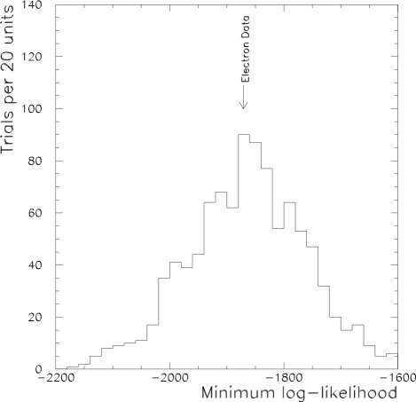
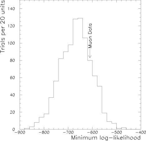
Figure 27: The minimum log-likelihood distributions of the toy Monte Carlo Left: Electrons Right: Muons.

The muon toy Monte Carlo samples have an input mean of $f_{towards}^{input}=34.5\%$ and a fit mean of $f_{towards}^{fit}=34.5\pm 0.4\%$. The width of the fit $f_{toward}$ distribution is $10.9\pm 0.3\%$, which is consistent with the error seen in data of ${}^{+9.2}_{-8.2}\%$. The electron toy Monte Carlo samples have an input mean of $f_{towards}^{input}=19.2\%$ and a fit mean of $f_{towards}^{fit}=18.6\pm 0.2\%$. The width of the fit $f_{toward}$ distribution is $6.0\pm 0.1$, which is consistent with the error seen in data of ${}^{+6.5}_{-5.8}\%$.

References

- Mangano et al. (1992) M. Mangano, P. Nason, and G. Ridolfi, Nucl. Phys. B373, 295 (1992).
- Albajar et al. (1991) C. Albajar et al., Phys. Lett. B256, 121 (1991).
- Abe et al. (1993a) F. Abe et al., Phys. Rev. Lett. 71, 500 (1993a).
- Abe et al. (1993b) F. Abe et al., Phys. Rev. Lett. 71, 2396 (1993b).
- Abe et al. (1995) F. Abe et al., Phys. Rev. Lett. 75, 1451 (1995).
- Acosta et al. (2002) D. Acosta et al., Phys. Rev. D65, 052005 (2002).
- Abachi et al. (1995) S. Abachi et al., Phys. Rev. Lett. 74, 3548 (1995).
- Abbott et al. (2000a) B. Abbott et al., Phys. Rev. Lett. 85, 5068 (2000a).
- Albajar et al. (1994) C. Albajar et al., Z. Phys. C61, 41 (1994).
- Abbott et al. (2000b) B. Abbott et al., Phys. Lett. B487, 264 (2000b).
- Abe et al. (1996) F. Abe et al., Phys. Rev. D53, 1051 (1996).
- Abe et al. (1997) F. Abe et al., Phys. Rev. D55, 2546 (1997).
- Cacciari and Nason (2002) M. Cacciari and P. Nason, Phys. Rev. Lett. 89, 122003 (2002).
- Halzen et al. (1983) F. Halzen, W. Y. Keung, and D. M. Scott, Phys. Rev. D27, 1631 (1983).
- Berger et al. (2001) E. L. Berger et al., Phys. Rev. Lett. 86, 4231 (2001).
- Acosta et al. (2004) D. Acosta et al., Phys. Rev. D69, 072004 (2004).
- Sjostrand and Bengtsson (1987) T. Sjostrand and M. Bengtsson, Comput. Phys. Comm. 43, 367 (1987).
- Bengtsson and Sjostrand (1987) H.-U. Bengtsson and T. Sjostrand, Comput. Phys. Comm. 46, 43 (1987).
- Marchesini et al. (1992) G. Marchesini et al., Comput. Phys. Comm. 67, 465 (1992).
- Field (2002) R. D. Field, Phys. Rev. D65, 094006 (2002).
- Abe et al. (1994a) F. Abe et al., Phys. Rev. D50, 2966 (1994a).
- Affolder et al. (2001) T. Affolder et al., Phys. Rev. D64, 032002 (2001).
- Abe et al. (1988a) F. Abe et al., Nucl. Instrum. Methods A271, 387 (1988a).
- Abe et al. (1988b) F. Abe et al., Nucl. Instrum. Methods A271, 387 (1988b).
- Cihangir et al. (1995) S. Cihangir et al., Nucl. Instrum. Methods A360, 137 (1995).
- Balka et al. (1988) L. Balka et al., Nucl. Instrum. Methods A267, 272 (1988).
- Bertolucci et al. (1988) S. Bertolucci et al., Nucl. Instrum. Methods A267, 301 (1988).
- Ascoli et al. (1988) G. Ascoli et al., Nucl. Instrum. Methods A268, 33 (1988).
- Brandenburg et al. (2002) G. Brandenburg et al., CDF public note 6362, CDF (2002).
- Abe et al. (1999) F. Abe et al., Phys. Rev. D60, 072003 (1999).
- Lannon (2003) K. Lannon, Ph.D. thesis, U. of Illinois at Urbana-Champaign (2003), http://library.fnal.gov/archive/thesis/fermilab-thesis-2003-21.pdf.
- Norrbin and Sjostrand (1998) E. Norrbin and T. Sjostrand, Phys. Lett. B442, 407 (1998), eprint hep-ph/9809266.
- Norrbin and Sjostrand (2000) E. Norrbin and T. Sjostrand, Eur. Phys. J. C17, 137 (2000), eprint hep-ph/0005110.
- (34) R. D. Field, Private communication, http://www.phys.ufl.edu/rfield.
- Avery et al. (1985) P. Avery et al., Cornell Internal Note CSN-112, CLEO (1985).
- Affolder et al. (2000a) T. Affolder et al., Phys. Rev. D61, 072005 (2000a).
- Abe et al. (1998a) F. Abe et al., Phys. Rev. D58, 112004 (1998a).
- Bardi et al. (2002) A. Bardi et al., Nucl. Instrum. Methods A485, 178 (2002).
- Marriner (1993) J. Marriner, CDF public note 1996, CDF (1993).
- Abe et al. (1998b) F. Abe et al., Phys. Rev. D57, 5382 (1998b).
- Affolder et al. (2000b) T. Affolder et al., Phys. Rev. Lett. 85, 2886 (2000b).
- Groom et al. (2000) D. E. Groom et al., Eur. Phys. J. C15, 1 (2000).
- Long (1998) O. Long, Ph.D. thesis, University of Pennsylvania (1998).
- Suzuki (1998) J. Suzuki, Ph.D. thesis, University of Tsukuba (1998).
- James and Roos (1975) F. James and M. Roos, Comput. Phys. Comm. 10, 343 (1975).
- Hagiwara et al. (2002) K. Hagiwara et al., Phys. Rev. D66, 010001 (2002).
- Abe et al. (2000) F. Abe et al., Phys. Rev. D61, 032001 (2000).
- Lai et al. (1995) H. L. Lai et al., Phys. Rev. D51, 4763 (1995).
- Martin et al. (1998) A. D. Martin et al., Eur. Phys. J. C4, 463 (1998).
- Apanasevich et al. (1999) L. Apanasevich et al., Phys. Rev. D59, 074007 (1999).
- Lai et al. (2000) H. L. Lai et al. (CTEQ), Eur. Phys. J. C12, 375 (2000), eprint hep-ph/9903282.
- Bowler (1981) M. G. Bowler, Z. Phys. C11, 169 (1981).
- Shapiro et al. (1992) M. Shapiro et al., CDF public note 1810, CDF (1992).
- Abe et al. (1994b) F. Abe et al., Phys. Rev. D50, 2966 (1994b).
- Braaten et al. (1993) E. Braaten et al., Phys. Rev. D48, 5049 (1993).
- Isgur et al. (1989) N. Isgur et al., Phys. Rev. D39, 799 (1989).
- Nason et al. (1989) P. Nason et al., Nucl. Phys. B327, 49 (1989).
- Peterson et al. (1983) C. Peterson et al., Phys. Rev. D27, 105 (1983).