CERN–PH-EP/2004-062

DELPHI Collaboration

Abstract

A novel high precision method measures the b-quark forward-backward asymmetry at the Z pole on a sample of 3,560,890 hadronic events collected with the DELPHI detector in 1992 to 2000. An enhanced impact parameter tag provides a high purity b sample. For event hemispheres with a reconstructed secondary vertex the charge of the corresponding quark or anti-quark is determined using a neural network which combines in an optimal way the full available charge information from the vertex charge, the jet charge and from identified leptons and hadrons. The probability of correctly identifying b-quarks and anti-quarks is measured on the data themselves comparing the rates of double hemisphere tagged like-sign and unlike-sign events. The b-quark forward-backward asymmetry is determined from the differential asymmetry, taking small corrections due to hemisphere correlations and background contributions into account. The results for different centre-of-mass energies are:

$A_{FB}^{{\mathrm{b}}}$ (89.449 GeV)	=	$0.0637\pm 0.0143(\mbox{stat.})\pm 0.0017(\mbox{syst.})$
$A_{FB}^{{\mathrm{b}}}$ (91.231 GeV)	=	$0.0958\pm 0.0032(\mbox{stat.})\pm 0.0014(\mbox{syst.})$
$A_{FB}^{{\mathrm{b}}}$ (92.990 GeV)	=	$0.1041\pm 0.0115(\mbox{stat.})\pm 0.0024(\mbox{syst.})$

Combining these results yields the b-quark pole asymmetry

$$A_{FB}^{{\mathrm{b,0}}}=0.0972\pm 0.0030(\mbox{stat.})\pm 0.0014(\mbox{syst.})$$

(Submitted to Eur. Phys. J. C)

J.Abdallah${}^{\ref{LPNHE}}$, P.Abreu${}^{\ref{LIP}}$, W.Adam${}^{\ref{VIENNA}}$, P.Adzic${}^{\ref{DEMOKRITOS}}$, Z.Albrecht${}^{\ref{KARLSRUHE}}$, T.Alderweireld${}^{\ref{AIM}}$, R.Alemany-Fernandez${}^{\ref{CERN}}$, T.Allmendinger${}^{\ref{KARLSRUHE}}$, P.P.Allport${}^{\ref{LIVERPOOL}}$, U.Amaldi${}^{\ref{MILANO2}}$, N.Amapane${}^{\ref{TORINO}}$, S.Amato${}^{\ref{UFRJ}}$, E.Anashkin${}^{\ref{PADOVA}}$, A.Andreazza${}^{\ref{MILANO}}$, S.Andringa${}^{\ref{LIP}}$, N.Anjos${}^{\ref{LIP}}$, P.Antilogus${}^{\ref{LPNHE}}$, W-D.Apel${}^{\ref{KARLSRUHE}}$, Y.Arnoud${}^{\ref{GRENOBLE}}$, S.Ask${}^{\ref{LUND}}$, B.Asman${}^{\ref{STOCKHOLM}}$, J.E.Augustin${}^{\ref{LPNHE}}$, A.Augustinus${}^{\ref{CERN}}$, P.Baillon${}^{\ref{CERN}}$, A.Ballestrero${}^{\ref{TORINOTH}}$, P.Bambade${}^{\ref{LAL}}$, R.Barbier${}^{\ref{LYON}}$, D.Bardin${}^{\ref{JINR}}$, G.Barker${}^{\ref{KARLSRUHE}}$, A.Baroncelli${}^{\ref{ROMA3}}$, M.Battaglia${}^{\ref{CERN}}$, M.Baubillier${}^{\ref{LPNHE}}$, K-H.Becks${}^{\ref{WUPPERTAL}}$, M.Begalli${}^{\ref{BRASIL}}$, A.Behrmann${}^{\ref{WUPPERTAL}}$, E.Ben-Haim${}^{\ref{LAL}}$, N.Benekos${}^{\ref{NTU-ATHENS}}$, A.Benvenuti${}^{\ref{BOLOGNA}}$, C.Berat${}^{\ref{GRENOBLE}}$, M.Berggren${}^{\ref{LPNHE}}$, L.Berntzon${}^{\ref{STOCKHOLM}}$, D.Bertrand${}^{\ref{AIM}}$, M.Besancon${}^{\ref{SACLAY}}$, N.Besson${}^{\ref{SACLAY}}$, D.Bloch${}^{\ref{CRN}}$, M.Blom${}^{\ref{NIKHEF}}$, M.Bluj${}^{\ref{WARSZAWA}}$, M.Bonesini${}^{\ref{MILANO2}}$, M.Boonekamp${}^{\ref{SACLAY}}$, P.S.L.Booth${}^{\ref{LIVERPOOL}}$, G.Borisov${}^{\ref{LANCASTER}}$, O.Botner${}^{\ref{UPPSALA}}$, B.Bouquet${}^{\ref{LAL}}$, T.J.V.Bowcock${}^{\ref{LIVERPOOL}}$, I.Boyko${}^{\ref{JINR}}$, M.Bracko${}^{\ref{SLOVENIJA}}$, R.Brenner${}^{\ref{UPPSALA}}$, E.Brodet${}^{\ref{OXFORD}}$, P.Bruckman${}^{\ref{KRAKOW1}}$, J.M.Brunet${}^{\ref{CDF}}$, P.Buschmann${}^{\ref{WUPPERTAL}}$, M.Calvi${}^{\ref{MILANO2}}$, T.Camporesi${}^{\ref{CERN}}$, V.Canale${}^{\ref{ROMA2}}$, F.Carena${}^{\ref{CERN}}$, N.Castro${}^{\ref{LIP}}$, F.Cavallo${}^{\ref{BOLOGNA}}$, M.Chapkin${}^{\ref{SERPUKHOV}}$, Ph.Charpentier${}^{\ref{CERN}}$, P.Checchia${}^{\ref{PADOVA}}$, R.Chierici${}^{\ref{CERN}}$, P.Chliapnikov${}^{\ref{SERPUKHOV}}$, J.Chudoba${}^{\ref{CERN}}$, S.U.Chung${}^{\ref{CERN}}$, K.Cieslik${}^{\ref{KRAKOW1}}$, P.Collins${}^{\ref{CERN}}$, R.Contri${}^{\ref{GENOVA}}$, G.Cosme${}^{\ref{LAL}}$, F.Cossutti${}^{\ref{TU}}$, M.J.Costa${}^{\ref{VALENCIA}}$, D.Crennell${}^{\ref{RAL}}$, J.Cuevas${}^{\ref{OVIEDO}}$, J.D’Hondt${}^{\ref{AIM}}$, J.Dalmau${}^{\ref{STOCKHOLM}}$, T.da Silva${}^{\ref{UFRJ}}$, W.Da Silva${}^{\ref{LPNHE}}$, G.Della Ricca${}^{\ref{TU}}$, A.De Angelis${}^{\ref{TU}}$, W.De Boer${}^{\ref{KARLSRUHE}}$, C.De Clercq${}^{\ref{AIM}}$, B.De Lotto${}^{\ref{TU}}$, N.De Maria${}^{\ref{TORINO}}$, A.De Min${}^{\ref{PADOVA}}$, L.de Paula${}^{\ref{UFRJ}}$, L.Di Ciaccio${}^{\ref{ROMA2}}$, A.Di Simone${}^{\ref{ROMA3}}$, K.Doroba${}^{\ref{WARSZAWA}}$, J.Drees${}^{\ref{WUPPERTAL},\ref{CERN}}$, M.Dris${}^{\ref{NTU-ATHENS}}$, G.Eigen${}^{\ref{BERGEN}}$, T.Ekelof${}^{\ref{UPPSALA}}$, M.Ellert${}^{\ref{UPPSALA}}$, M.Elsing${}^{\ref{CERN}}$, M.C.Espirito Santo${}^{\ref{LIP}}$, G.Fanourakis${}^{\ref{DEMOKRITOS}}$, D.Fassouliotis${}^{\ref{DEMOKRITOS},\ref{ATHENS}}$, M.Feindt${}^{\ref{KARLSRUHE}}$, J.Fernandez${}^{\ref{SANTANDER}}$, A.Ferrer${}^{\ref{VALENCIA}}$, F.Ferro${}^{\ref{GENOVA}}$, U.Flagmeyer${}^{\ref{WUPPERTAL}}$, H.Foeth${}^{\ref{CERN}}$, E.Fokitis${}^{\ref{NTU-ATHENS}}$, F.Fulda-Quenzer${}^{\ref{LAL}}$, J.Fuster${}^{\ref{VALENCIA}}$, M.Gandelman${}^{\ref{UFRJ}}$, C.Garcia${}^{\ref{VALENCIA}}$, Ph.Gavillet${}^{\ref{CERN}}$, E.Gazis${}^{\ref{NTU-ATHENS}}$, R.Gokieli${}^{\ref{CERN},\ref{WARSZAWA}}$, B.Golob${}^{\ref{SLOVENIJA}}$, G.Gomez-Ceballos${}^{\ref{SANTANDER}}$, P.Goncalves${}^{\ref{LIP}}$, E.Graziani${}^{\ref{ROMA3}}$, G.Grosdidier${}^{\ref{LAL}}$, K.Grzelak${}^{\ref{WARSZAWA}}$, J.Guy${}^{\ref{RAL}}$, C.Haag${}^{\ref{KARLSRUHE}}$, A.Hallgren${}^{\ref{UPPSALA}}$, K.Hamacher${}^{\ref{WUPPERTAL}}$, K.Hamilton${}^{\ref{OXFORD}}$, S.Haug${}^{\ref{OSLO}}$, F.Hauler${}^{\ref{KARLSRUHE}}$, V.Hedberg${}^{\ref{LUND}}$, M.Hennecke${}^{\ref{KARLSRUHE}}$, H.Herr${}^{\ref{CERN}}$, J.Hoffman${}^{\ref{WARSZAWA}}$, S-O.Holmgren${}^{\ref{STOCKHOLM}}$, P.J.Holt${}^{\ref{CERN}}$, M.A.Houlden${}^{\ref{LIVERPOOL}}$, K.Hultqvist${}^{\ref{STOCKHOLM}}$, J.N.Jackson${}^{\ref{LIVERPOOL}}$, G.Jarlskog${}^{\ref{LUND}}$, P.Jarry${}^{\ref{SACLAY}}$, D.Jeans${}^{\ref{OXFORD}}$, E.K.Johansson${}^{\ref{STOCKHOLM}}$, P.D.Johansson${}^{\ref{STOCKHOLM}}$, P.Jonsson${}^{\ref{LYON}}$, C.Joram${}^{\ref{CERN}}$, L.Jungermann${}^{\ref{KARLSRUHE}}$, F.Kapusta${}^{\ref{LPNHE}}$, S.Katsanevas${}^{\ref{LYON}}$, E.Katsoufis${}^{\ref{NTU-ATHENS}}$, G.Kernel${}^{\ref{SLOVENIJA}}$, B.P.Kersevan${}^{\ref{CERN},\ref{SLOVENIJA}}$, U.Kerzel${}^{\ref{KARLSRUHE}}$, A.Kiiskinen${}^{\ref{HELSINKI}}$, B.T.King${}^{\ref{LIVERPOOL}}$, N.J.Kjaer${}^{\ref{CERN}}$, P.Kluit${}^{\ref{NIKHEF}}$, P.Kokkinias${}^{\ref{DEMOKRITOS}}$, C.Kourkoumelis${}^{\ref{ATHENS}}$, O.Kouznetsov${}^{\ref{JINR}}$, Z.Krumstein${}^{\ref{JINR}}$, M.Kucharczyk${}^{\ref{KRAKOW1}}$, J.Lamsa${}^{\ref{AMES}}$, G.Leder${}^{\ref{VIENNA}}$, F.Ledroit${}^{\ref{GRENOBLE}}$, L.Leinonen${}^{\ref{STOCKHOLM}}$, R.Leitner${}^{\ref{NC}}$, J.Lemonne${}^{\ref{AIM}}$, V.Lepeltier${}^{\ref{LAL}}$, T.Lesiak${}^{\ref{KRAKOW1}}$, W.Liebig${}^{\ref{WUPPERTAL}}$, D.Liko${}^{\ref{VIENNA}}$, A.Lipniacka${}^{\ref{STOCKHOLM}}$, J.H.Lopes${}^{\ref{UFRJ}}$, J.M.Lopez${}^{\ref{OVIEDO}}$, D.Loukas${}^{\ref{DEMOKRITOS}}$, P.Lutz${}^{\ref{SACLAY}}$, L.Lyons${}^{\ref{OXFORD}}$, J.MacNaughton${}^{\ref{VIENNA}}$, A.Malek${}^{\ref{WUPPERTAL}}$, S.Maltezos${}^{\ref{NTU-ATHENS}}$, F.Mandl${}^{\ref{VIENNA}}$, J.Marco${}^{\ref{SANTANDER}}$, R.Marco${}^{\ref{SANTANDER}}$, B.Marechal${}^{\ref{UFRJ}}$, M.Margoni${}^{\ref{PADOVA}}$, J-C.Marin${}^{\ref{CERN}}$, C.Mariotti${}^{\ref{CERN}}$, A.Markou${}^{\ref{DEMOKRITOS}}$, C.Martinez-Rivero${}^{\ref{SANTANDER}}$, J.Masik${}^{\ref{FZU}}$, N.Mastroyiannopoulos${}^{\ref{DEMOKRITOS}}$, F.Matorras${}^{\ref{SANTANDER}}$, C.Matteuzzi${}^{\ref{MILANO2}}$, F.Mazzucato${}^{\ref{PADOVA}}$, M.Mazzucato${}^{\ref{PADOVA}}$, R.Mc Nulty${}^{\ref{LIVERPOOL}}$, C.Meroni${}^{\ref{MILANO}}$, E.Migliore${}^{\ref{TORINO}}$, W.Mitaroff${}^{\ref{VIENNA}}$, U.Mjoernmark${}^{\ref{LUND}}$, T.Moa${}^{\ref{STOCKHOLM}}$, M.Moch${}^{\ref{KARLSRUHE}}$, K.Moenig${}^{\ref{CERN},\ref{DESY}}$, R.Monge${}^{\ref{GENOVA}}$, J.Montenegro${}^{\ref{NIKHEF}}$, D.Moraes${}^{\ref{UFRJ}}$, S.Moreno${}^{\ref{LIP}}$, P.Morettini${}^{\ref{GENOVA}}$, U.Mueller${}^{\ref{WUPPERTAL}}$, K.Muenich${}^{\ref{WUPPERTAL}}$, M.Mulders${}^{\ref{NIKHEF}}$, L.Mundim${}^{\ref{BRASIL}}$, W.Murray${}^{\ref{RAL}}$, B.Muryn${}^{\ref{KRAKOW2}}$, G.Myatt${}^{\ref{OXFORD}}$, T.Myklebust${}^{\ref{OSLO}}$, M.Nassiakou${}^{\ref{DEMOKRITOS}}$, F.Navarria${}^{\ref{BOLOGNA}}$, K.Nawrocki${}^{\ref{WARSZAWA}}$, R.Nicolaidou${}^{\ref{SACLAY}}$, M.Nikolenko${}^{\ref{JINR},\ref{CRN}}$, A.Oblakowska-Mucha${}^{\ref{KRAKOW2}}$, V.Obraztsov${}^{\ref{SERPUKHOV}}$, A.Olshevski${}^{\ref{JINR}}$, A.Onofre${}^{\ref{LIP}}$, R.Orava${}^{\ref{HELSINKI}}$, K.Osterberg${}^{\ref{HELSINKI}}$, A.Ouraou${}^{\ref{SACLAY}}$, A.Oyanguren${}^{\ref{VALENCIA}}$, M.Paganoni${}^{\ref{MILANO2}}$, S.Paiano${}^{\ref{BOLOGNA}}$, J.P.Palacios${}^{\ref{LIVERPOOL}}$, H.Palka${}^{\ref{KRAKOW1}}$, Th.D.Papadopoulou${}^{\ref{NTU-ATHENS}}$, L.Pape${}^{\ref{CERN}}$, C.Parkes${}^{\ref{GLASGOW}}$, F.Parodi${}^{\ref{GENOVA}}$, U.Parzefall${}^{\ref{CERN}}$, A.Passeri${}^{\ref{ROMA3}}$, O.Passon${}^{\ref{WUPPERTAL}}$, L.Peralta${}^{\ref{LIP}}$, V.Perepelitsa${}^{\ref{VALENCIA}}$, A.Perrotta${}^{\ref{BOLOGNA}}$, A.Petrolini${}^{\ref{GENOVA}}$, J.Piedra${}^{\ref{SANTANDER}}$, L.Pieri${}^{\ref{ROMA3}}$, F.Pierre${}^{\ref{SACLAY}}$, M.Pimenta${}^{\ref{LIP}}$, E.Piotto${}^{\ref{CERN}}$, T.Podobnik${}^{\ref{SLOVENIJA}}$, V.Poireau${}^{\ref{CERN}}$, M.E.Pol${}^{\ref{BRASIL}}$, G.Polok${}^{\ref{KRAKOW1}}$, P.Poropat^†${}^{\ref{TU}}$, V.Pozdniakov${}^{\ref{JINR}}$, N.Pukhaeva${}^{\ref{AIM},\ref{JINR}}$, A.Pullia${}^{\ref{MILANO2}}$, J.Rames${}^{\ref{FZU}}$, L.Ramler${}^{\ref{KARLSRUHE}}$, A.Read${}^{\ref{OSLO}}$, P.Rebecchi${}^{\ref{CERN}}$, J.Rehn${}^{\ref{KARLSRUHE}}$, D.Reid${}^{\ref{NIKHEF}}$, R.Reinhardt${}^{\ref{WUPPERTAL}}$, P.Renton${}^{\ref{OXFORD}}$, F.Richard${}^{\ref{LAL}}$, J.Ridky${}^{\ref{FZU}}$, M.Rivero${}^{\ref{SANTANDER}}$, D.Rodriguez${}^{\ref{SANTANDER}}$, A.Romero${}^{\ref{TORINO}}$, P.Ronchese${}^{\ref{PADOVA}}$, P.Roudeau${}^{\ref{LAL}}$, T.Rovelli${}^{\ref{BOLOGNA}}$, V.Ruhlmann-Kleider${}^{\ref{SACLAY}}$, D.Ryabtchikov${}^{\ref{SERPUKHOV}}$, A.Sadovsky${}^{\ref{JINR}}$, L.Salmi${}^{\ref{HELSINKI}}$, J.Salt${}^{\ref{VALENCIA}}$, A.Savoy-Navarro${}^{\ref{LPNHE}}$, T.Scheidle${}^{\ref{KARLSRUHE}}$, B.Schwering${}^{\ref{WUPPERTAL},\ref{AACHEN}}$, U.Schwickerath${}^{\ref{CERN}}$, A.Segar${}^{\ref{OXFORD}}$, R.Sekulin${}^{\ref{RAL}}$, M.Siebel${}^{\ref{WUPPERTAL}}$, A.Sisakian${}^{\ref{JINR}}$, G.Smadja${}^{\ref{LYON}}$, O.Smirnova${}^{\ref{LUND}}$, A.Sokolov${}^{\ref{SERPUKHOV}}$, A.Sopczak${}^{\ref{LANCASTER}}$, R.Sosnowski${}^{\ref{WARSZAWA}}$, T.Spassov${}^{\ref{CERN}}$, M.Stanitzki${}^{\ref{KARLSRUHE}}$, A.Stocchi${}^{\ref{LAL}}$, J.Strauss${}^{\ref{VIENNA}}$, B.Stugu${}^{\ref{BERGEN}}$, M.Szczekowski${}^{\ref{WARSZAWA}}$, M.Szeptycka${}^{\ref{WARSZAWA}}$, T.Szumlak${}^{\ref{KRAKOW2}}$, T.Tabarelli${}^{\ref{MILANO2}}$, A.C.Taffard${}^{\ref{LIVERPOOL}}$, F.Tegenfeldt${}^{\ref{UPPSALA}}$, J.Timmermans${}^{\ref{NIKHEF}}$, L.Tkatchev${}^{\ref{JINR}}$, M.Tobin${}^{\ref{LIVERPOOL}}$, S.Todorovova${}^{\ref{FZU}}$, B.Tome${}^{\ref{LIP}}$, A.Tonazzo${}^{\ref{MILANO2}}$, P.Tortosa${}^{\ref{VALENCIA}}$, P.Travnicek${}^{\ref{FZU}}$, D.Treille${}^{\ref{CERN}}$, G.Tristram${}^{\ref{CDF}}$, M.Trochimczuk${}^{\ref{WARSZAWA}}$, C.Troncon${}^{\ref{MILANO}}$, M-L.Turluer${}^{\ref{SACLAY}}$, I.A.Tyapkin${}^{\ref{JINR}}$, P.Tyapkin${}^{\ref{JINR}}$, S.Tzamarias${}^{\ref{DEMOKRITOS}}$, V.Uvarov${}^{\ref{SERPUKHOV}}$, G.Valenti${}^{\ref{BOLOGNA}}$, P.Van Dam${}^{\ref{NIKHEF}}$, J.Van Eldik${}^{\ref{CERN}}$, A.Van Lysebetten${}^{\ref{AIM}}$, N.van Remortel${}^{\ref{AIM}}$, I.Van Vulpen${}^{\ref{CERN}}$, G.Vegni${}^{\ref{MILANO}}$, F.Veloso${}^{\ref{LIP}}$, W.Venus${}^{\ref{RAL}}$, P.Verdier${}^{\ref{LYON}}$, V.Verzi${}^{\ref{ROMA2}}$, D.Vilanova${}^{\ref{SACLAY}}$, L.Vitale${}^{\ref{TU}}$, V.Vrba${}^{\ref{FZU}}$, H.Wahlen${}^{\ref{WUPPERTAL}}$, A.J.Washbrook${}^{\ref{LIVERPOOL}}$, C.Weiser${}^{\ref{KARLSRUHE}}$, D.Wicke${}^{\ref{CERN}}$, J.Wickens${}^{\ref{AIM}}$, G.Wilkinson${}^{\ref{OXFORD}}$, M.Winter${}^{\ref{CRN}}$, M.Witek${}^{\ref{KRAKOW1}}$, O.Yushchenko${}^{\ref{SERPUKHOV}}$, A.Zalewska${}^{\ref{KRAKOW1}}$, P.Zalewski${}^{\ref{WARSZAWA}}$, D.Zavrtanik${}^{\ref{SLOVENIJA}}$, V.Zhuravlov${}^{\ref{JINR}}$, N.I.Zimin${}^{\ref{JINR}}$, A.Zintchenko${}^{\ref{JINR}}$, M.Zupan${}^{\ref{DEMOKRITOS}}$

1 Introduction

The measurements of the b-quark forward-backward asymmetry at the Z pole provide the most precise determination of the effective electroweak mixing angle, ${\mathrm{sin}}^{2}\theta_{\mathrm{eff}}^{\ell}$, at LEP. For pure Z exchange and to lowest order the forward-backward pole asymmetry of b-quarks, $A_{FB}^{0,{\mathrm{b}}}$, can be written in terms of the vector and axial-vector couplings of the initial electrons ($v_{{\mathrm{e}}},a_{{\mathrm{e}}}$) and the final b-quarks ($v_{{\mathrm{b}}},a_{{\mathrm{b}}}$):

$$\mbox{\begin{math}A_{FB}^{0,{\mathrm{b}}}\end{math}}={3\over 4}\frac{2a_{{\mathrm{e}}}v_{{\mathrm{e}}}}{a_{{\mathrm{e}}}^{2}+v_{{\mathrm{e}}}^{2}}\frac{2a_{{\mathrm{b}}}v_{{\mathrm{b}}}}{a_{{\mathrm{b}}}^{2}+v_{{\mathrm{b}}}^{2}}$$ (1)

Higher order electroweak corrections are taken into account by means of an improved Born approximation [1], which leaves the above relation unchanged, but defines the modified couplings ($\bar{a}_{{\mathrm{f}}}$, $\bar{v}_{{\mathrm{f}}}$) and an effective mixing angle $\theta^{\mathrm{f}}_{\mathrm{e}ff}$:

$$\frac{\bar{v}_{{\mathrm{f}}}}{\bar{a}_{{\mathrm{f}}}}=1-4|q_{{\mathrm{f}}}|\sin^{2}\theta^{\mathrm{f}}_{\mathrm{e}ff}$$ (2)

using the electric charge $q_{{\mathrm{f}}}$ of the fermion. The b-quark forward-backward asymmetry determines the ratio of these couplings. It is essentially only sensitive to ${\mathrm{sin}}^{2}\theta_{\mathrm{eff}}^{\ell}$ defined by the ratio of the electron couplings.

Previously established methods to measure the b-quark forward-backward asymmetry in DELPHI [2, 3] either exploited the charge correlation of the semileptonic decay lepton (muon or electron) to the initial b charge or used the jet charge information in selected b events. These methods suffer from either the limited efficiency, because of the relatively small semileptonic branching ratio or from the limited charge tagging performance because of the small jet charge separation between a b-quark and anti-quark jet.

The present analysis improves on the charge tagging performance by using the full available experimental charge information from b jets. Such an improvement is achievable because of the different sensitivities of charged and neutral b hadrons to the original b-quark, and because of the separation between fragmentation and decay charge. The excellent DELPHI microvertex detector separates the particles from B decays from fragmentation products on the basis of the impact parameter measurement. The hadron identification capability, facilitated by the DELPHI Ring Imaging CHerenkov counters (RICH), provides a means of exploiting charge correlations of kaons or baryons in b jets. Thus, not only can the secondary b decay vertex charge be measured directly but also further information for a single jet, like the decay flavour for the different B types ($\mathrm{B}^{0}$, $\mathrm{B}^{+}$, $\mathrm{B}_{s}$ and b baryon), can be obtained. A set of Neural Networks is used to combine the additional input with the jet and vertex charge information in an optimal way.

2 Principles of the method to extract the b asymmetry

The differential cross-section for b-quarks from the process $\mathrm{e}^{+}\mathrm{e}^{-}\rightarrow\mbox{Z}\rightarrow\mbox{b}\overline{\mbox{b}}$ as a function of the polar angle $\theta$ can be expressed as :

$$\frac{d\sigma}{d\cos\theta}\propto 1+\frac{8}{3}\,A_{FB}^{{\mathrm{b}}}\,\cos\theta+\cos^{2}\theta\,.$$ (3)

Hence the forward-backward asymmetry generates a linear $\cos\theta$ dependence in the production of b-quarks. For anti-quarks the orientation (sign) of the production angle is reversed.

The thrust axis is used to approximate the quark direction in the analysis [4]. The plane perpendicular to the thrust axis defines the two event hemispheres. The charge of the primary quark or anti-quark in a hemisphere is necessary to determine the orientation of the quark polar angle $\theta_{\vec{T}}$. This charge information can be obtained separately for both event hemispheres using the hemisphere charge Neural Network output.

In order to exploit the much improved b charge tagging fully, a self-calibrated method to extract the forward-backward asymmetry has been developed. The b-quark charge sign is measured in event hemispheres with a reconstructed secondary vertex. The different possible combinations of negative, positive and untagged event hemispheres define classes of single and double charge tagged events, with the double tagged distinguished into like-sign and unlike-sign. The forward and backward rates of single and double unlike-sign events provide sensitivity to the asymmetry. As the $\mbox{b}\overline{\mbox{b}}$ final state is neutral, one of the two hemispheres in like-sign events is known to be mistagged. By comparing the like-sign and unlike-sign rates of double hemisphere charge tagged events it is hence possible to extract the probability of correctly assigning the b-quark charge directly from the data.

A b-tagging variable constructed from lifetime information as well as secondary vertex and track observables provides an additional strong means of rejecting charm and light quark events in which a secondary vertex occurred. Separate event samples of successively enhanced b purity are used in the analysis to allow for a statistical correlation between the b purity and the probability of correctly assigning the quark charge.

The asymmetry measurement as well as the self-calibration method rely on the good knowledge of the true b content and residual non-b background in the individual rates of differently charge-tagged events. Therefore the b efficiency in each rate is measured directly on the real data. For the most important background contribution, c-quark events, additional calibration techniques are used: the c-quark efficiency of the enhanced impact parameter tag is measured using a double tag method while the c charge tagging probability is calibrated on data by means of D decays reconstructed in the opposite hemisphere.

The b-quark forward-backward asymmetry is determined from the differential asymmetry of the two classes of single tagged and unlike-sign double tagged events. The differential asymmetry is measured independently in consecutive bins of the polar angle and in the different b purity samples. Here small corrections due to residual background contributions and due to charge tagging hemisphere correlations are taken into account.

The paper is organised as follows. First a short summary of the hadronic event selection is given. In Section 4 the b event tagging used to obtain the high-purity b-quark sample is described in conjunction with the calibration of its efficiency. Section 5 details the charge tagging technique using Neural Networks and the self-calibrating method to extract the forward-backward asymmetry. Section 6 describes the measurement of $A_{FB}^{{\mathrm{b}}}$ from the DELPHI data of 1992 to 2000. Section 7 discusses the systematic errors. Finally the conclusion is given in Section 8, and combined final values on $A_{FB}^{{\mathrm{b}}}$ and $A_{FB}^{{\mathrm{c}}}$ are presented in Section 9. Technical information on the self-calibration method can be found in the appendix.

3 Selection of Z decays to hadrons

A detailed description of the DELPHI apparatus for both the LEP 1 and LEP 2 phases can be found in [5] and in the references therein. This analysis makes full use of the information provided by the tracking system, the calorimetry and the detectors for hadron and lepton identification. Of special importance is the silicon Vertex Detector providing three precise $R\phi$ measurements. For the years 1992 to 1993 the lowest polar angle $\theta$ for obtaining at least one $R\phi$ measurement is $31^{\circ}$, while for the years 1994 to 1995 the enhanced detector measured particles down to a $\theta$ of $25^{\circ}$ and provided additional $z$ measurements in the outer shell and the shell close to the beam [6]. From 1996 onwards the fully replaced DELPHI silicon tracker provided $R\phi$ and $z$ measurements down to a $\theta$ of $21^{\circ}$. For the exact number of measurements as a function of polar and azimuthal angles we refer to reference [7].

This analysis uses all the DELPHI data taken from 1992 to 2000 at centre-of-mass energies close to the Z pole. In addition to the LEP 1 data in an interval of $\pm 0.5$ GeV around the Z pole, the data taken at $2$ GeV above and below as well as the LEP 2 calibration runs taken at the Z pole are included. The different years and centre-of-mass energies divide the data into nine sets which are analysed separately and compared to individually generated simulated data.

For events entering the analysis, nominal working conditions during data taking are required at least for the central tracking detector, a Time Projection Chamber (TPC), for the electromagnetic calorimeters and for the barrel muon detector system. The operating conditions and efficiency of the RICH detectors varied widely for the different data sets. These variations are included in the corresponding simulated data samples.

charged particle momentum	$\geq$	$0.4\,$ GeV/$c$
neutral particle energy	see text
length of tracks measured only with TPC	$\geq$	$30\,$cm
polar angle	$\geq$	$20^{\circ}$
uncertainty of the momentum measured	$\leq$	$100\,\%$
impact parameter ($R\phi$)	$\leq$	$4\,$cm
impact parameter ($z$)	$\leq$	$10\,$cm

Table 1: Cuts to select particles. Impact parameters are defined relative to the primary vertex.

For each event cuts are applied to the measured particles to ensure both good quality of the reconstruction and also good agreement of data and simulation. The selections are summarised in Table 1. In addition, for neutral clusters measured in the calorimeters the reconstructed shower energy had to be above 0.3 GeV for the barrel electromagnetic calorimeter (HPC) and the small angle luminosity calorimeters (STIC/SAT), and above 0.4 GeV for the Forward ElectroMagnetic Calorimeter (FEMC).

A second step selects Z decays to hadrons as detailed in Table 2. Here each event is divided into two hemispheres by the plane perpendicular to the thrust axis $\vec{T}$ which is computed using the charged and neutral particles. $\theta_{\vec{T}}$ is the polar angle of the thrust axis. In addition, the negligible number of events with an unphysically high momentum particle are discarded.

In total $3.56\cdot 10^{6}$ Z decays to hadrons are selected using data from mean centre-of-mass energies of 89.449 GeV, 91.231 GeV and 92.990 GeV (see Table 3). The data taking periods with centre-of-mass energies below and above the Z peak (called “peak-2” and “peak+2” in the following) are analysed separately. The remaining backgrounds due to $\tau\tau$, Bhabha, and $\gamma\gamma$ events as well as contributions from beam-gas or beam-wall interactions are estimated to be below $0.5\,\%$. After the subsequent selection of Z decays to b-quarks with a reconstructed secondary vertex, they are safely neglected.

The data are compared to $10.43\cdot 10^{6}$ fully simulated hadronic decays using JETSET 7.3 [8] with DELPHI tuning of fragmentation, b production and decay parameters [9].

 

total energy of charged particles	$\geq$	$0.15\times\sqrt{s}$
sum of energy of charged particles in a hemisphere	$\geq$	$0.03\times\sqrt{s}$
total multiplicity of charged particles	$\geq$	$7$
multiplicity of charged particles in hemisphere	$\geq$	$1$
forward electromagnetic energy $E_{\mbox{\tiny{\,FEMC}}}:=\sqrt{E_{\mbox{\tiny{\,F}}}^{2}+E_{\mbox{\tiny{\,B}}}^{2}}\qquad\qquad$	$\leq$	$85\%\,E_{\mbox{\tiny{\,beam}}}$

Table 2: Selections for Z decays to hadrons. $\sqrt{s}$ is the centre-of-mass energy, $E_{\mbox{\tiny{\,F/B}}}$ the total shower energy per FEMC side.

year	data	simulation	$\langle\sqrt{s}\rangle$
1992	636401	1827321	91.280 GeV
1993	454895	1901060	91.225 GeV
1994	1303131	3260752	91.202 GeV
1995	416560	1206974	91.288 GeV
1996-2000	332944	971299	91.260 GeV
1993 peak-2	86601	269027	89.431 GeV
1993 peak+2	126648	339528	93.015 GeV
1995 peak-2	79989	268899	89.468 GeV
1995 peak+2	123721	385648	92.965 GeV

Table 3: Number of selected (data) and generated (simulation) Z decays to hadrons for the different years of data taking and different centre-of-mass energies.

4 Selection of Z decays to b-quarks using an enhanced impact parameter method

4.1 The b tagging method

Decays to b-quarks are selected from the sample of hadronic Z decays using the DELPHI high-purity b tagging technique. It is based on the well established hemisphere b-tag method used by DELPHI for the precision measurement of $R_{{\mathrm{b}}}$ [10, 11]. The analysis uses the apparent lifetime calculated from the track impact parameters, information from the decay vertex when it is reconstructed and the rapidities of charged particles. The latter are defined with respect to the jet direction as reconstructed with the LUCLUS algorithm [8]. The information from the secondary decay vertex consists of the invariant mass, the transverse momentum, and the energy fraction of the decay products. All the variables are combined into one discriminator which is defined independently in each of the event hemispheres. Since the uncertainty from modelling the correlation between the b-tag hemispheres only has a small impact on this measurement, a common event primary vertex is used.

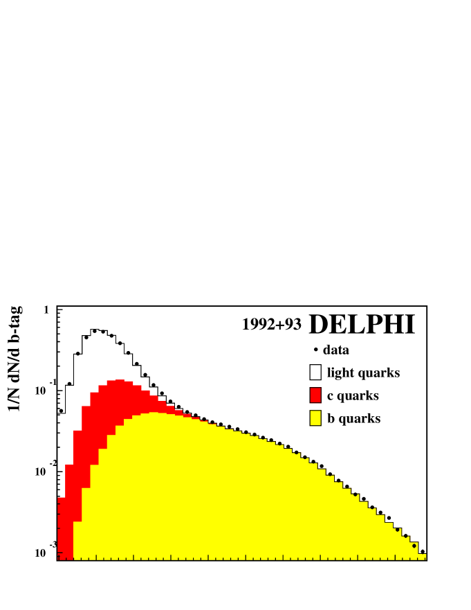
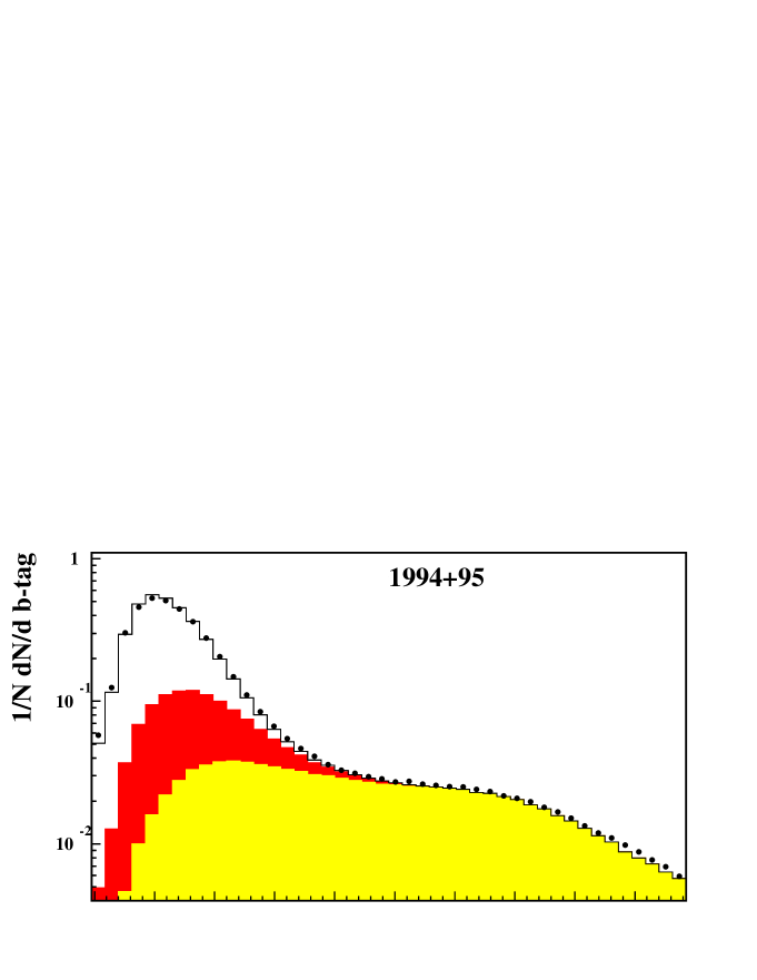
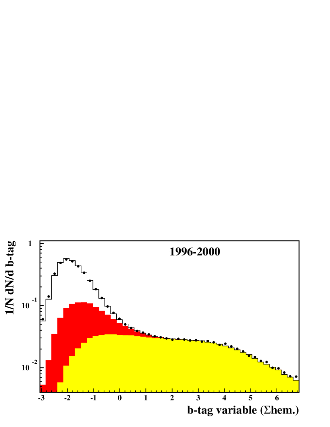
Figure 1: Comparison between data and simulation of the normalised number of events versus the b-tag variable for 1992+93 (upper plot), 1994+95 (middle) and 1996-2000 (lower plot). The b-, c- and light quark composition of the simulation has been reweighted according to the measured branching fractions [12]. The b- and c-quark simulation correction from Section 4.3 is not applied at this stage.

This analysis uses an event tagging probability variable, b-tag, made of the sum of the two hemisphere discriminators. With an allowed range from $-5.0$ to $10.0$, decays to b-quarks tend to have higher b-tag values whereas decays to other quarks are peaked at smaller values as can be seen in Figure 1, separately for the combined years 1992 + 93, 1994 + 95 and 1996-2000. High-purity samples are selected by cutting on ${b\mbox{-}tag}>-0.2$ for 1992 + 93 and ${b\mbox{-}tag}>0.0$ for 1994 to 2000. This guarantees a working point at constant b purity over the years regardless of the change in tagging performance due to the differences in the VD set-up. The selected sample is divided into four consecutive bins with increasing b purity, as detailed in Table 5.3 in Section 5.3, to allow for correlations between the charge tagging and the b purity.

The inputs to the tagging variable depend on detector resolution as well as on b and c hadron decay properties and lifetimes. Their limited knowledge leads to an imperfect description of the tagging performance in the simulation. To avoid a resulting bias in the background estimates, the simulation is calibrated on the data in several steps, before the efficiencies and purities relevant for extracting $A_{FB}^{{\mathrm{b}}}$ on the b-enriched charge tagged samples are calculated.

First, an accurate tuning of the resolution in the simulation to the one in data has been performed [10, 11] in order to estimate the c and light flavour background efficiencies correctly. Here each year of data taking is treated separately to allow for the changes in the detector performance. The simulated data have also been reweighted in order to represent the measured composition and lifetimes of charmed and beauty hadrons and also the rate of gluon splitting into $\mbox{c}\overline{\mbox{c}}$ ($\mbox{b}\overline{\mbox{b}}$) pairs correctly.

After that the b and c efficiencies on the b-enriched samples are calibrated by means of a double tagging method similar to the one which has been used in the $R_{b}$ measurement to derive $R_{\mathrm{b}}$ and the b efficiency simultaneously [11]. Its special application to this analysis corrects the fractions of b- and c-quarks and is described in the following sections.

The event b efficiency and the flavour fractions are then calculated for every data subsample entering the $A_{FB}^{{\mathrm{b}}}$ measurement. Knowing precisely the real b efficiency and purity in different event categories is essential to further self-calibration by deriving simultaneously $A_{FB}^{{\mathrm{b}}}$ and the probability to tag the charge of the b decay correctly.

4.2 The b tagging efficiency calibration to b and c events

Since the b-tagging variable is defined independently in each hemisphere, a double tagging method can be applied to calibrate the simulated b and c selection efficiencies on the data. The selection efficiencies, $\varepsilon_{i}$, modify the fractions of b, c and uds events, which are initially the fractions of b and c events produced in hadronic ${\mathrm{Z}}$ decays, $R_{{\mathrm{b}}}$ and $R_{{\mathrm{c}}}$. This applies likewise to hemispheres, where the fraction with b-tag${}_{\mbox{\tiny hem}}$ variable $x$ larger than some cut value $x_{0}$ can be written as,

$$\frac{N^{x>x_{0}}}{N^{tot}}={\mathcal{F}}^{x>x_{0}}=R_{\mathrm{b}}\cdot{\varepsilon_{{\mathrm{b}}}^{\mathrm{hem.}}}+R_{\mathrm{c}}\cdot{\varepsilon_{{\mathrm{c}}}^{\mathrm{hem.}}}+(1-R_{{\mathrm{c}}}-R_{{\mathrm{b}}})\cdot{\varepsilon_{\mathrm{uds}}^{\mathrm{hem.}}}$$ (4)

where $N^{tot}$ is the initial number of hemispheres and ${{\varepsilon_{{\mathrm{j}}}^{\mathrm{hem.}}}}$ the selection efficiency for each flavour. For example, ${\varepsilon_{{\mathrm{c}}}^{\mathrm{hem.}}}$ is the efficiency to tag a real c event hemisphere as a “b”.

Since each event has 2 hemispheres, such a selection defines three different kinds of event: double b-tagged events where both hemispheres have a b-tag${}_{\mbox{\tiny hem}}$ value bigger than the selection-cut, single b-tagged events where only one hemisphere is larger than the cut and no b-tagged events where both hemispheres are below the selection cut. The fraction of double, single and no-tagged are therefore,

$${\mathcal{F}}\mbox{\boldmath${}^{d}$} = R_{\mathrm{b}}\cdot{\varepsilon_{\mathrm{b}}}^{d}+R_{\mathrm{c}}\cdot{\varepsilon_{\mathrm{c}}}^{d}+(1-R_{{\mathrm{c}}}-R_{{\mathrm{b}}})\cdot{\varepsilon_{\mathrm{uds}}}^{d}$$ (5)

$${\mathcal{F}}\mbox{\boldmath${}^{s}$} = R_{\mathrm{b}}\cdot{\varepsilon_{\mathrm{b}}}^{s}+R_{\mathrm{c}}\cdot{\varepsilon_{\mathrm{c}}}^{s}+(1-R_{{\mathrm{c}}}-R_{{\mathrm{b}}})\cdot{\varepsilon_{\mathrm{uds}}}^{s}$$ (6)

$${\mathcal{F}}\mbox{\boldmath${}^{n}$} = R_{\mathrm{b}}\cdot{\varepsilon_{\mathrm{b}}}^{n}+R_{\mathrm{c}}\cdot{\varepsilon_{\mathrm{c}}}^{n}+(1-R_{{\mathrm{c}}}-R_{{\mathrm{b}}})\cdot{\varepsilon_{\mathrm{uds}}}^{n}.$$ (7)

By definition $\sum_{j}{\mathcal{F}}^{j}=1$ and so only two of these equations are independent. The selection efficiencies of the three different kinds of event depend on the product of the two hemisphere selection efficiencies and the correlation that exists between them. This correlation, $k$, is defined such that a value of $0$ implies the hemispheres are uncorrelated whereas $\,k=1\,$ means that the hemispheres are fully correlated. The dependence of the event efficiencies on the single-hemisphere selection efficiency and on $k_{{\mathrm{j}}}$ is given below where index ${\mathrm{j}}$ runs over the three flavour types; b, c and uds.

$$\varepsilon^{d}_{{\mathrm{j}}} = {{\varepsilon_{{\mathrm{j}}}^{\mathrm{hem.}}}}\ k_{{\mathrm{j}}}+({{\varepsilon_{{\mathrm{j}}}^{\mathrm{hem.}}}})^{2}(1-k_{{\mathrm{j}}})$$ (8)

$$\varepsilon^{s}_{{\mathrm{j}}} = 2{{\varepsilon_{{\mathrm{j}}}^{\mathrm{hem.}}}}(1-k_{{\mathrm{j}}})-2({{\varepsilon_{{\mathrm{j}}}^{\mathrm{hem.}}}})^{2}(1-k_{{\mathrm{j}}})$$ (9)

$$\varepsilon^{n}_{{\mathrm{j}}} = 1-{{\varepsilon_{{\mathrm{j}}}^{\mathrm{hem.}}}}(2-k_{{\mathrm{j}}})+({{\varepsilon_{{\mathrm{j}}}^{\mathrm{hem.}}}})^{2}(1-k_{{\mathrm{j}}})\ \ .$$ (10)

The method involves solving equations (5)-(7) for ${\varepsilon_{{\mathrm{b}}}^{\mathrm{hem.}}}$ and ${\varepsilon_{{\mathrm{c}}}^{\mathrm{hem.}}}$ with the replacement of the modified efficiencies of equations (8)-(10). The solution obtained on simulated data yields the correlations $k_{{\mathrm{j}}}$ by solving equations (8)-(10). For real data, the fractions of double, single and no-tagged events are measured, but the efficiency for uds events and the $k_{{\mathrm{j}}}$ are taken from simulation. This method measures the selection efficiency for b and c hemispheres directly with the data. The resulting efficiencies can then be compared with the corresponding quantities in the simulation and a correction function formed from any difference seen. This function is then used to bring the simulated b and c selection efficiencies into agreement with those measured in real data. The correction is formed and applied separately for b and c hemispheres.

  

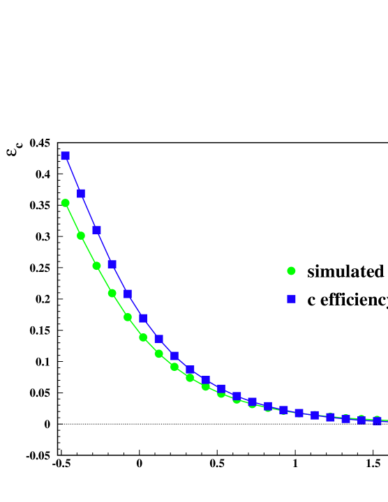
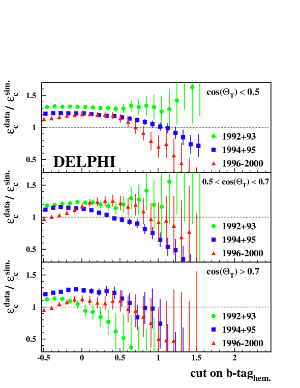
Figure 2: The measured efficiency of c-quark hemispheres, as a function of the cut on b-tag${}_{\mbox{\tiny hem}}$, in simulation compared to real data following the procedure outlined in the text. The upper plot details the situation in the central region for the 1994+95 data, while the triple plot below summarises the agreement found in all three VD set-ups and polar angle ranges.

4.3 The correction function

Among the different steps to calibrate and measure the b selection efficiency, only the previously introduced double b tag method gives access to the c efficiency on real data. The measured c selection efficiencies in simulation and real data are shown in the upper part of Figure 2 for the example of the 1994+95 central region at $\cos\theta_{\vec{T}}<0.5$. The displayed range for the cut on the b-tag${}_{\mbox{\tiny hem}}$ variable represents the interval where c-quarks are the dominant background contribution for this analysis and where the efficiency calibration for b and c events is performed. It is found that in a low b-tag${}_{\mbox{\tiny hem}}$ region where the c background forms an important contribution, the simulation underestimates the amount of c-quarks entering the sample. This observation is expected to vary between the different set-ups for the vertex detector and its angular acceptance. In the lower part of Figure 2 the ratio of real to simulated c efficiency is shown for 1992 + 93, 1994 + 95 and 1996-2000 as well as for the angular regions of $\cos\theta_{\vec{T}}<0.5$, $\cos\theta_{\vec{T}}\in[0.5,0.7]$ and $\cos\theta_{\vec{T}}\geq 0.7$ .

The correction function used to calibrate the simulated b and c efficiencies is constructed individually on those set-ups and regions studied in Figure 2, thus taking the slightly different data to simulation ratios into account. Its construction is illustrated in the sketch in Figure 3, which mirrors the situation found in Figure 2. For each bin in b-tag${}_{\mbox{\tiny hem}}$, a correction is applied to the b-tag${}_{\mbox{\tiny hem}}$ value in simulated b and c hemispheres in order to force the data and simulation efficiency curves into agreement.

The correction at the level of the whole event is then accounted for by simply adding together the corrected b-tag${}_{\mbox{\tiny hem}}$ values of the two event hemispheres. The result of applying such a correction function is shown in Figure 4 which plots the data to simulation ratio for the integrated b-tag at event level. The simulation is found to agree with data within $\pm 1\,\%$. Uncertainties on the remaining modelling input to the correction function, such as hemisphere correlations and residual uds background are taken into account in the study of systematic uncertainties.

Figure 3: Construction of the correction function for each bin.

Figure 4: The (integrated) b-tag ratio of real to simulated events after application of the correction functions to simulated b- and c-quark events. The data are from the 1994+95 DELPHI data set. Different correction functions for the $\cos\theta_{\vec{T}}$ intervals of $[0.0,0.5]$, $[0.5,0.7]$ and $\geq 0.7$ were applied before integrating over the full polar angle.

5 The inclusive charge tagging

This section explains the novel method for inclusive b charge tagging. First the experimental information and the Neural Network technique used to extract the b-quark charge information from the DELPHI data are described. In the second part the self-calibrating method to extract the b-quark forward-backward asymmetry is explained. This includes the technique to determine the tagging probabilities for b-quark events as well as for the main background of c-quark events. Also charge correlations between the two event hemispheres are discussed.

5.1 The Neural Network method for inclusive charge tagging

The analysis uses the full available experimental charge information from b jets which is combined into one tagging variable using a Neural Network technique. The tagging method and all prior steps of extracting the charge information from b jets are part of a DELPHI analysis package for b physics called Bsaurus. In this paper only an overview of the package is given. Full details can be found in reference [13].

The hemisphere charge tagging Neural Network is designed to distinguish between hemispheres originating from the b-quark or anti-quark in Z $\to\mbox{b}\overline{\mbox{b}}$ decays and thus to provide the essential information to measure the asymmetry. For b jets with a reconstructed secondary vertex it combines jet charge and vertex charge information with so-called b-hadron flavour tags, quantities that reconstruct the b-quark charge at the time of production and, if possible, also at the time of decay for any given b-hadron hypothesis. Before the ingredients for the final hemisphere charge tagging Network are described in Section 5.1.3 the basic requirements such as secondary vertex finding and forming the b-hadron flavour tags are outlined.

5.1.1 Secondary vertex finding

Obtaining a Network output in the hemisphere under consideration requires the presence of a secondary B or D decay vertex, which is reconstructed in a two-stage iterative method. The first stage selects tracks with quality criteria similar to those in Table 1 and discriminates between tracks originating from the secondary vertex or from fragmentation using lifetime and kinematic information as well as particle identification. Starting from this track list, the secondary and primary vertex positions are simultaneously fitted in three dimensions, using the event primary vertex as a starting point and constraining the secondary vertex to the flight direction of the b-hadron. If the fit did not pass certain convergence criteria, the track making the largest $\chi^{2}$ contribution is ignored and the fit repeated in an iterative procedure. Once a convergent fit has been attained, the second stage involves an attempt to rebuild and extend the lists of tracks in the fit using as discriminator the output of an interim version of the TrackNet that is described in Section 5.1.2. Tracks that did not pass the initial selection criteria, but are nevertheless consistent with originating from one of the vertices, are iteratively included in this stage, and retained if the new fit converges.

5.1.2 The construction of the b-hadron flavour tags

The motivation behind forming the b-hadron flavour tags is to use in an optimal way the information contained in the particle charge. Its interpretation depends, however, on the type of b-hadron present in the jet. For example, an identified proton in a jet containing a b baryon often carries information about the b-quark charge, while for b mesons it does not. This approach works by constructing first a conditional probability on the track level: the probability $P^{time}(same\,sign\,|\,{\mathrm{B}})$ for a given track to have the same charge sign as the b-quark in a given b-hadron type (${\mathrm{B}}^{0}$, ${\mathrm{B}}^{+}$, ${\mathrm{B}}_{s}$ and b baryon). They are defined for both the time of fragmentation (i.e. production) and the time of decay.

To discriminate fragmentation from decay tracks, a Neural Network called TrackNet separates particles originating from the event primary vertex from those starting at a secondary decay vertex. The separation uses the impact parameter measurement and additional kinematic information. Particles from the primary vertex lead to TrackNet values close to 0, while particles from a secondary vertex get values close to 1.

Dedicated Neural Networks are trained for each of the four b-hadron types, and for each set two separate versions are produced: one trained only on tracks originating from the fragmentation process, and the other trained only on tracks originating from the weak b-hadron decay. This construction makes the final charge tagging Network explicitly sensitive to information that is specific to a particular ${\mathrm{B}}$ hadron type. Various effects, such as the proton charge in the fragmentation tracks of b baryon jets often being anticorrelated to the b charge, or ${\mathrm{B}}-\overline{{\mathrm{B}}}$ oscillations between neutral ${\mathrm{B}}$ production and decay, are taken into account automatically. The Networks themselves are defined such that the target output value is $+1$ $(-1)$ if the charge of a particle is correlated (anti-correlated) to the b-quark charge. A set of predefined input variables is used to establish the correlation:

• Particle identification variables.
  Lepton and hadron identification information is combined into tagging variables for kaons, protons, electrons, and muons. The charge of direct leptons is fully correlated to the quark charge in b, c or ${\mathrm{b}}{}\!\to\!{\mathrm{c}}$ decays, while for example a high-energy kaon can carry charge information via the decay chain ${\mathrm{b}}\!\to\!{\mathrm{c}}\!\to\!{\mathrm{s}}$. The kaon information needs to be weighted differently by the Networks for ${\mathrm{B}}^{0}$ and ${\mathrm{B}}_{s}$ hadrons because in the case of ${\mathrm{B}}_{s}$ additional kaons can be present.

• B-D separation.
  The above examples also show that the Networks must be able to separate particles from the weak B decay from those from the subsequent cascade D decay. This information is supplied by a dedicated Neural Network called BD-Net which uses decay vertex and kinematic information in a given jet. The BD-Net absolute value and the output value in relation to the spectrum of BD-Net outputs for the other tracks in the hemisphere are both inputs to the decay-track version of the Networks.

• Kinematic and topological variables are also used to decide if a track is likely to be correlated to the b-quark charge. They are the energy of the particle and, after boosting into the estimated B candidate rest frame, the momentum and angle of the particle in that frame.

• Quality variables.
  Further variables characterising the quality of the track and the associated B candidate are input to the Networks. The number of charged particles assigned to secondary vertices in the hemisphere with TrackNet above 0.5 and the uncertainty on the vertex charge measurement are used. Other inputs are the presence of ambiguities in track reconstruction, as well as kinematic information about the reconstructed B candidate and the $\chi^{2}$ probability of the fit for the B decay vertex.

The particle correlation conditional probabilities, $P^{time}(same\,sign\,|\,{\mathrm{B}})$, for the fragmentation and the decay flavour are then combined using a likelihood ratio to obtain a flavour tag for a given hemisphere:

$$F_{\mathrm{B}}^{time}=\sum_{\mathrm{particles}}\ln\left(\frac{1+P^{time}(same\,sign\,|\,{\mathrm{B}})}{1-P^{time}(same\,sign\,|\,{\mathrm{B}})}\right)\cdot Q~{}.$$ (11)

Here B is either a ${\mathrm{B}^{+},\mathrm{B}^{0},\mathrm{B}_{s}}$ or b baryon and $time$ stands for fragmentation or decay. $Q$ is the particle charge. Depending on the hypothesis considered a different selection is applied for particles entering the summation. For the fragmentation (decay) flavour tag all tracks with TrackNet${}<0.5$ (${}\geq 0.5$) are considered.

5.1.3 The final hemisphere charge tagging Neural Network $flav_{\mbox{\tiny hem}}$

Nine different inputs for the final hemisphere charge Neural Network are constructed. The first set of inputs is a combination of the fragmentation (Frag.) and decay (Dec.) b-hadron flavour tags multiplied by the individual probabilities for that b-hadron type (ignoring some details of variable transformation and re-scaling):

• $F_{\mathrm{B}_{s}}^{Frag.}\cdot P(\mathrm{B}_{s})$

• $\left(F_{\mathrm{B}^{+}}^{Dec.}-F_{\mathrm{B}^{+}}^{Frag.}\right)\cdot P(\mathrm{B}^{+})$

• $\left(F_{baryon}^{Dec.}-F_{baryon}^{Frag.}\right)\cdot P(baryon)$

• $\left(F_{\mathrm{B}^{0}}^{Dec.}\cdot\left(1-2\sin^{2}(\frac{\Delta(m_{d})}{2}\cdot\tau_{\mathrm{rec}})\right)-F_{\mathrm{B}^{0}}^{Frag.}\right)\cdot P(\mathrm{B}^{0})$

Here $\tau_{\mathrm{rec}}$ is the reconstructed proper B lifetime in the hemisphere under consideration. The construction considers the $\mathrm{B}^{0}$ oscillation frequency which affects the charge information in the hemisphere. It is assumed to be $\Delta(m_{\mathrm{d}})=0.474\,/\mathrm{ps}$. This is not possible for the case of $\mathrm{B}_{s}$ where the oscillations are so fast that at the time of decay a 50-50 mix of $\mathrm{B}_{s}$ and $\overline{\mathrm{B}}_{s}$ remains.

The $P({\mathrm{B}})$ factors are the outputs of a dedicated B species identification Network which represent probabilities that the hemisphere in question contains a weakly decaying b-hadron of a particular type B. They are constructed such that on the average their sum is 1, but as they are used to form a new Network input this constraint is not applied on a single measurement.

The remaining inputs are:

• The so-called jet charge defined as:

  $$Q_{J}=\frac{\sum_{\mathrm{particles}}p_{L}^{\kappa}\cdot Q}{\sum_{\mathrm{particles}}p_{L}^{\kappa}},$$ (12)

  where the sum is over all charged particles in a hemisphere and $p_{L}$ is the longitudinal momentum component with respect to the thrust axis. The optimal choice of the free parameter $\kappa$ depends on the type of b-hadron under consideration. Therefore a range of values ($\kappa=0.3,0.6,\infty$) are used, where the last one corresponds to taking the charge of the highest momentum particle in the hemisphere.

• The vertex charge is constructed using the TrackNet value as a probability for each track to originate from the b-hadron decay vertex. The weighted vertex charge is formed by:

  $$Q_{\mathrm{V}}=\sum_{\mathrm{particles}}\mbox{TrackNet}\cdot Q~{}.$$ (13)

• The significance $Q_{\mathrm{V}}/\sigma(Q_{\mathrm{V}})$ of the vertex charge calculated using a binomial error estimator:

  $$\sigma(Q_{\mathrm{V}})=\sqrt{\sum_{\mathrm{particles}}\mbox{TrackNet}\cdot(1-\mbox{TrackNet})}~{}.$$ (14)

As an example the distributions of the jet charge for $\kappa=0.3$ and $0.6$ and of the vertex charge and its significance are shown in Figure 5 for data and simulation.

Figure 5: The jet charge information for $\kappa=0.3$ and $0.6$ (upper plots) and the vertex charge and its significance (lower plot). Shown is the comparison between 1994 data and simulation for all hemispheres that are both b and charge tagged.

In addition to the charge discriminating variables described above, use is made of ‘quality’ variables, e.g. the reconstructed energy of the B candidate in the hemisphere. These inputs supply the network during the training process with information regarding the likely quality of the discriminating variables, and are implemented in the form of weights to the turn-on gradient (or ‘temperature’) of the sigmoid function used as network node transfer function. (See, for example, reference [14] for discussion of these concepts.)

The training of the networks uses a standard feed-forward algorithm. The final network utilises an architecture of 9 input nodes, one for each of the variables defined above, a hidden layer containing 10 nodes and one output node. During the training, the target values at the output node for one hemisphere were $-1$ for a b-quark or $+1$ for a b anti-quark.

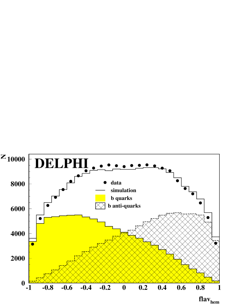
Figure 6: Comparison between data and simulation for the hemisphere charge tag Neural Network output, ${flav_{\mbox{\tiny hem}}}$, for the data of 1994. Hemispheres from all b-enhanced samples were used, resulting in a b purity of $90\,\%$.

An example of the hemisphere charge Neural Network output, ${flav_{\mbox{\tiny hem}}}$, on the selected high-purity b event sample is shown in Figure 6 for the data of 1994. The data points are compared to the simulation. The contributions from hemispheres containing b-quarks and anti-quarks are shown separately for the simulation to illustrate the excellent charge separation. The difference between data and simulation in the width of the distribution indicates a small difference in the charge tagging efficiency which will be discussed in detail in Sections 5.4 and 5.6.

In the analysis a hemisphere is charge tagged, if a secondary vertex is sufficiently well reconstructed to produce a Neural Network output ${flav_{\mbox{\tiny hem}}}$ and if the absolute value $|{flav_{\mbox{\tiny hem}}}|$  exceeds the work point cut of 0.35 (0.30 in case of 1992 + 93 data). This working point was chosen to minimise the expected relative error of the measured b asymmetry on simulated data.

5.2 The method to extract the b asymmetry

5.2.1 Single and double charge tagged events

The Neural Network charge tag is used to reconstruct the charge sign of the primary b-quark on a per-hemisphere basis. Different categories are distinguished according to the configuration of the two charge-signed hemispheres in an event.

In single charge tagged events the orientation of the primary quark axis is obtained from the sign of the tagged hemisphere’s Neural Network output. The quark axis is forward oriented ($\cos\theta_{\vec{T}}>0$) if a forward hemisphere is tagged to contain a b-quark or a backward hemisphere is tagged to contain a b anti-quark. Otherwise the quark axis is backward ($\cos\theta_{\vec{T}}<0$) oriented.

One needs to distinguish two categories of events if both hemispheres are charge tagged. Events with one hemisphere tagged as quark and the other as anti-quark belong to the category of unlike-sign double charge tagged. Here the event orientation is determined by either hemisphere. The situation is similar to single hemisphere events, but the additional second hemisphere charge tag increases the probability to identify the sign of the quark charge correctly. By contrast, events for which both hemispheres are tagged to contain quarks (or both anti-quarks) do not have a preferred orientation. These like-sign events are used to measure the charge tagging probability.

5.2.2 The observed asymmetry

The difference between the number of forward and backward events normalised to the sum is the forward-backward asymmetry. Thus for single hemisphere tag events:

$$A_{FB}^{obs}\,=\,\frac{{N}-{\overline{N}}}{{N}+{\overline{N}}}\,=\,\sum\limits_{{\mathrm{f}}={\mathrm{d}},{\mathrm{u}},{\mathrm{s}},{\mathrm{c}},{\mathrm{b}}}(2\cdot w_{{\mathrm{f}}}-1)\cdot{A_{FB}^{{\mathrm{f}}}}\cdot{p_{{\mathrm{f}}}}\cdot\eta_{\mathrm{f}}\ ,$$ (15)

where

${N}$	=	number of forward events with a single charge tag,
${\overline{N}}$	=	number of backward events with a single charge tag.

Similarly for the double charge tagged events:

$$A_{FB}^{D,obs}\,=\,\frac{{N^{D}}-{\overline{N^{D}}}}{{N^{D}}+{\overline{N^{D}}}}\,=\,\sum\limits_{{\mathrm{f}}={\mathrm{d}},{\mathrm{u}},{\mathrm{s}},{\mathrm{c}},{\mathrm{b}}}(2\cdot w_{{\mathrm{f}}}^{D}-1)\cdot{A_{FB}^{{\mathrm{f}}}}\cdot{p_{{\mathrm{f}}}^{D}}\cdot\eta_{\mathrm{f}}\ ,$$ (16)

where

${N^{D}}$	=	number of forward events with a double charge tag,
${\overline{N^{D}}}$	=	number of backward events with a double charge tag.

The observed asymmetry is the sum of the contributions from b events and from c and uds background events. $A_{FB}^{{\mathrm{f}}}$ is the forward-backward asymmetry, ${p_{{\mathrm{f}}}}$ and ${p_{{\mathrm{f}}}^{D}}$ are the fractions for each flavour in the single and double unlike-sign tagged event categories. The $\eta$-term accounts for the differently signed charge asymmetries, $\eta_{\mathrm{f}}=-1$ for up-type quarks and $\eta_{\mathrm{f}}=1$ for down-type quarks.

The quantities $w_{{\mathrm{f}}}$ and $w_{{\mathrm{f}}}^{D}$ are the probabilities to identify the sign of the quark charge correctly in single and double tagged simulated events. For simulated events they can be determined directly by exploiting the truth information, whether the sign of the underlying quark charge is correctly reconstructed by the charge tag. For single tagged events:

$${w_{{\mathrm{f}}}}=\frac{{\hat{N}_{{\mathrm{f}}}}+{\hat{N}_{\overline{\mathrm{f}}}}}{{N_{{\mathrm{f}}}}+{N_{\overline{\mathrm{f}}}}}~{}~{},$$ (17)

where ${N_{{\mathrm{f}}}}({N_{\overline{\mathrm{f}}}})$ is the number of events tagged as quark (anti-quark) by the single hemisphere providing the ${flav_{\mbox{\tiny hem}}}$ output. ${\hat{N}_{{\mathrm{f}}}}({\hat{N}_{\overline{\mathrm{f}}}})$ is the number of events in which the quark (anti-quark) has been correctly identified.

For unlike-sign events the fraction of events, in which both quark and anti-quark charges are correctly identified, is defined analogously to the single charge tagged events as the ratio of correctly tagged (${\hat{N}_{{\mathrm{f}}}^{D}},{\hat{N}_{\overline{\mathrm{f}}}^{D}}$) over all double-tagged unlike-sign (${N_{{\mathrm{f}}}^{D}},{N_{\overline{\mathrm{f}}}^{D}}$) events:

$${w_{{\mathrm{f}}}^{D}}=\frac{{\hat{N}_{{\mathrm{f}}}^{D}}+{\hat{N}_{\overline{\mathrm{f}}}^{D}}}{{N_{{\mathrm{f}}}^{D}}+{N_{\overline{\mathrm{f}}}^{D}}}~{}~{}.$$ (18)

To measure the b-quark forward-backward asymmetry all quantities appearing in Equations 15 and 16 have to be determined. The equations are applied in bins of the polar angle, as will be explained in Section 6. The rates $N$, $\overline{N}$, $N^{D}$, $\overline{N^{D}}$ are obtained from the data. The ${\mathrm{b}}$ purity, $p_{{\mathrm{b}}}$, and the probability to identify the b-quark charge correctly can also be extracted directly from data with only minimal input from simulation. The determination of $p_{{\mathrm{b}}}$ and the measurement of $w_{{\mathrm{b}}}^{(D)}$ and $w_{{\mathrm{c}}}^{(D)}$ are discussed in the next sections. Small corrections due to light quark background and to hemisphere correlations (see Sections 4.2 and 5.5) are based on simulation.

5.3 Calculation of the b efficiency and flavour fractions

The selection of events in single and double charge tagged categories biases the selection efficiencies and flavour fractions calibrated in Section 4.2. The measurement of $A_{FB}^{{\mathrm{b}}}$ needs the final selection efficiencies which take into account the complete selection after both ${b\mbox{-}tag}$ and charge tag in a given bin in $\cos\theta_{\vec{T}}$. The efficiency for selecting b-quark events, $\epsilon_{{\mathrm{b}}}$, and the corresponding fractions of b, c and light flavours are directly obtained from the data. $\epsilon_{{\mathrm{b}}}$ is calculated using:

$$\epsilon_{{\mathrm{b}}}(\mathrm{cut})=\frac{{\cal F}(\mathrm{cut})-R_{{\mathrm{c}}}\times\epsilon_{{\mathrm{c}}}(\mathrm{cut})-(1-R_{{\mathrm{c}}}-R_{{\mathrm{b}}})\times\epsilon_{\mathrm{uds}}(\mathrm{cut})}{R_{{\mathrm{b}}}}~{},$$ (19)

where ${\cal F}(\mathrm{cut})$ is the fraction of events selected on the data by any given cut. $\epsilon_{\mathrm{uds}}$ is the simulated selection efficiency for the light flavours while $\epsilon_{{\mathrm{c}}}$ for charm events is obtained from the simulation which has been calibrated using the correction function. The fractions of c and b events produced in hadronic ${\mathrm{Z}}$ decays, $R_{{\mathrm{c}}}$ and $R_{{\mathrm{b}}}$, are set to the LEP+SLD average values of $R_{{\mathrm{c}}}^{0}=0.1719\pm 0.0031$ and $R_{{\mathrm{b}}}^{0}=0.21644\pm 0.00065$ which are used throughout the whole analysis [12]. For the off-peak energy points the LEP+SLD on-peak values are extrapolated using Zfitter [15].

The corresponding fractions, $p_{{\mathrm{f}}}$, are then calculated for each flavour using:

$$p_{{\mathrm{f}}}(\mathrm{cut})=\epsilon_{{\mathrm{f}}}(\mathrm{cut})\times\frac{R_{{\mathrm{f}}}}{{\cal F}(\mathrm{cut})}~{}.$$ (20)

The combined data sample of single and unlike-sign double charge tagged events contains an average b fraction $p_{{\mathrm{b}}}$ of close to $90\,\%$ after the complete selection. Table 5.3 shows the measured $p_{{\mathrm{b}}}$ values broken down into years of data-taking and intervals in b-tag.

Figure 7: The b efficiencies $\epsilon_{{\mathrm{b}}}$ and $\epsilon_{{\mathrm{b}}}^{D}$ and the purities $p_{{\mathrm{b}}}$ and $p_{{\mathrm{b}}}^{D}$ for single and double unlike-sign tagged events as a function of the polar angle. The full sample of all four bins in b-tag has been used. The purity $p_{{\mathrm{b}}}^{same}$ for double like-sign tagged events is relevant for measuring the charge tagging probability, $w_{{\mathrm{b}}}^{(D)}$.

In Figure 7 the $\cos\theta_{\vec{T}}$ dependence of the b efficiencies $\epsilon_{{\mathrm{b}}}$ and $\epsilon_{{\mathrm{b}}}^{D}$ and b purities $p_{{\mathrm{b}}}$ and $p_{{\mathrm{b}}}^{D}$ is shown. The b purity $p_{{\mathrm{b}}}^{same}$ of the like-sign double tagged events is also included, as it is important for the self calibration method Equation 23. Both efficiency and purity are stable in the central region of the detector. At large $\cos\theta_{\vec{T}}$ the purity increases slowly for both categories of single and double tagged events. At the same time the b efficiency decreases with a fast drop for $\cos\theta_{\vec{T}}>0.7$. This drop is due to a decreasing detector performance for the b tagging. While events with a clear b signature are still tagged, the charm and light quark efficiencies drop even more, causing the b purity to rise.

For single tag events, the measured efficiency and purity are well predicted by simulation especially in the central region of the detector. The rates of like- and unlike-sign double tagged events provide sensitivity to the probability, $w_{{\mathrm{b}}}^{(D)}$, of identifying the quark charge correctly. As will be discussed in Section 5.4, $w_{{\mathrm{b}}}^{(D)}$ is calculated from ${p_{{\mathrm{b}}}^{D}}$ and ${p_{{\mathrm{b}}}^{same}}$. Hence the $1\,\%$ deviations between simulation and data, which are visible in Figure 7, propagate to $w_{{\mathrm{b}}}^{(D)}$ and require the calibrated probabilities to be used in the analysis.

	$-0.2\kern-0.90005pt<\kern-1.34995ptx\kern-1.34995pt<\kern-0.90005pt0.8$		$0.8<x<1.9$		$1.9<x<3.0$		$3.0<x<\infty$
1992	0.787 $\pm$	0.009	0.960 $\pm$	0.012	0.992 $\pm$	0.014	0.998 $\pm$	0.014
1993	0.773 $\pm$	0.011	0.956 $\pm$	0.014	0.990 $\pm$	0.016	0.998 $\pm$	0.016
	$0.0<x<1.2$		$1.2<x<2.3$		$2.3<x<3.4$		$3.4<x<\infty$
1994	0.712 $\pm$	0.006	0.952 $\pm$	0.009	0.989 $\pm$	0.009	0.997 $\pm$	0.006
1995	0.729 $\pm$	0.011	0.952 $\pm$	0.015	0.988 $\pm$	0.016	0.997 $\pm$	0.011
1996-2000	0.756 $\pm$	0.013	0.964 $\pm$	0.017	0.993 $\pm$	0.017	0.998 $\pm$	0.012

[The measured b purities for the different years and b-tag intervals] The measured b purities, or fractions, for the different years and intervals in $x\kern-1.20007pt:=\kern-1.20007pt{b\mbox{-}tag}{}$. The purities found for the off-peak data match the corresponding peak values well within errors.

5.4 The probabilities to identify the b-quark charge correctly

For the case of b-quarks the probabilities, $w_{{\mathrm{b}}}^{(D)}$, to identify the charge correctly can be measured directly from the data leading to a self-calibration of the analysis. The principle idea of the method is that the unlike-sign and like-sign double tagged events are proportional to:

$${N^{D}}+{\overline{N^{D}}}\propto\big{[}w_{{\mathrm{b}}}^{2}+(1-w_{{\mathrm{b}}})^{2}\big{]}~{},\vspace*{-2ex}$$ (21)

$${N^{same}}\propto 2\cdot w_{{\mathrm{b}}}\cdot(1-w_{{\mathrm{b}}})~{}.$$ (22)

where

${N^{same}}$	=	number of double tagged like-sign events.

Solving the quadratic equations and taking into account background leads to:

$${w_{{\mathrm{b}}}}\cdot\sqrt{1+\delta}=\frac{1}{2}+\sqrt{\frac{1}{4}-\frac{1}{2}\cdot\frac{{N^{same}}\cdot{p_{{\mathrm{b}}}^{same}}}{\big{[}{N^{D}}+{\overline{N^{D}}}\,\big{]}\cdot{p_{{\mathrm{b}}}^{D}}+{N^{same}}\cdot{p_{{\mathrm{b}}}^{same}}}}~{},$$ (23)

$${w_{{\mathrm{b}}}^{D}}\cdot\sqrt{1+\beta}=\frac{{w_{{\mathrm{b}}}}^{2}\cdot(1+\delta)}{{w_{{\mathrm{b}}}}^{2}\cdot(1+\delta)+(1-w_{{\mathrm{b}}}\cdot\sqrt{1+\delta})^{2}}~{}.$$ (24)

A detailed derivation of these equations can be found in the appendix. $p_{{\mathrm{b}}}^{D}$  and $p_{{\mathrm{b}}}^{same}$  are the b purities determined individually for the unlike-sign and like-sign categories using equations 19 and 20. The additional terms $\sqrt{1+\delta}$ and $\sqrt{1+\beta}$ allow for hemisphere charge correlations and are discussed in Section 5.5.

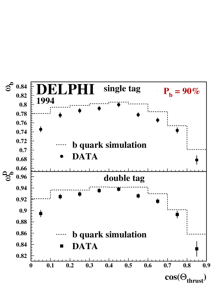
Figure 8: The probability to identify b-quarks correctly for data and simulation for the year 1994. The upper plot shows the result for single tagged events, the lower for double tagged events. See text for details.

In Figure 8 the measured probabilities for single and double tagged events are shown as a function of the polar angle for the year 1994. The results on data are corrected for background contributions and are compared to the prediction from simulation. In double tagged events $w_{{\mathrm{b}}}^{D}$ rises to be above $93\,\%$ and drops to $83\,\%$ for large $\cos\theta_{\vec{T}}$ near the edge of the detector acceptance. A similar shape with a maximum of $80\,\%$ is found for the single tagged events. The plot shows that the relative discrepancy between simulated and measured $w_{{\mathrm{b}}}^{(D)}$ is at the percent level, slightly varying with polar angle. This overall tendency to predict the real charge tagging power a little too high was observed regardless of b purity working point or year.

The different values for $w_{{\mathrm{b}}}$ and $w_{{\mathrm{b}}}^{D}$ shown in Figure 8 reflect the sensitivity to the quark charge in the two event categories: although there are 2.4 times more selected b events single-tagged than double unlike-sign tagged, the weight of the single-tagged events in the determination of $A_{FB}^{{\mathrm{b}}}$ is only $49\,\%$. In a study to exploit further the charge tag as a weight and thus improve on the statistical error, the analysis has been performed on different classes defined by intervals in the absolute value $|{flav_{\mbox{\tiny hem}}}|$, taking into account varying sensitivities to the quark charge between each class. This approach was dropped, because the resulting gain in the statistical error of the modified analysis is negligible while losing the good control of calibration techniques and residual systematic uncertainties.

5.5 The correlations $\delta$ and $\beta$

The probabilities to identify the quark charge correctly are deduced from double charge tagged like-sign and unlike-sign events. Correlations between the two hemisphere charge tags affect the measurement and need to be taken into account. The term $\sqrt{1+\delta}$ in Equation 23 allows for such correlations when calculating the single tag probability, $w_{{\mathrm{b}}}$, using the double tagged events. The probability to identify the quark charge in double tagged unlike-sign events, $w_{{\mathrm{b}}}^{D}$, is obtained from $w_{{\mathrm{b}}}$ using Equation 24. Here the additional term $\sqrt{1+\beta}$ allows for the different correlations in unlike-sign events.

Figure 9: Hemisphere charge correlation of single and double tagged simulated events for the years 1992 to 2000.

The correlation terms $\sqrt{1+\delta}$ and $\sqrt{1+\beta}$ are obtained from simulation using b-quark events. For that purpose, the result of the right hand side of Equation 23 is compared to the true tagging probability for single tagged events calculated using the simulation truth. The ratio of both results is given by the term $\sqrt{1+\delta}$. Similarly the term $\sqrt{1+\beta}$ is deduced from the ratio of the result from the right hand side of Equation 24 and the truth in double tagged unlike-sign events. In Figure 9 the correlations $\delta$ (upper plot) and $\beta$ (lower plot) are shown as a function of the polar angle $\cos{\theta_{\vec{T}}}$ for the different years of data taking. Within errors the correlations are stable as a function of the polar angle.

Figure 10: The mean of the correlations $\delta$ and $\beta$ of 1994 simulation as a function of the cut on the charge tag output $|{flav_{\mbox{\tiny hem}}}|$. Besides the full hemisphere charge network (points) results using modified networks without the jet charge input for $\kappa=0.3$ and both with an additional cut on the thrust value, $|\vec{T}|>0.9$, are shown. The statistical uncertainties on the quantities represented by lines are not drawn, but they are slightly larger than those shown for the points.

Possible sources of the hemisphere charge correlation have been investigated in detail. In order to understand the origin of the correlations, experimental input variables were consecutively discarded from the charge tagging Neural Network. With the charge tagging modified in this way, the measurement was repeated. Only for the charge network for which the jet charge for $\kappa=0.3$ was omitted was a significant variation in the correlation observed. The mean of the correlations $\langle\delta\rangle$ and $\langle\beta\rangle$ calculated with this version of the charge tag are shown as dashed lines in Figure 10. This can be compared to the dependence of the correlation for the full Neural Network as a function of the cut on the charge tag output $|{flav_{\mbox{\tiny hem}}}|$, which is shown as points. Almost no correlations for $\langle\delta\rangle$ and $\langle\beta\rangle$ remain after removing the jet charge information with the lowest $\kappa$ parameter.

The source of hemisphere charge correlations for the jet charge analysis has been studied in reference [2]. It was found that the dominant sources of correlations are charge conservation in the event and QCD effects introduced by gluon radiation. The charge conservation effect is found to be most pronounced for $\kappa=0.3$, which gives highest weights to soft tracks; the same behaviour is found for the charge tagging Neural Network. The hemisphere charge correlations $\delta$ and $\beta$ are also sensitive to gluon radiation. This behaviour is illustrated in Figure 10 by applying a cut on the thrust value of $|\vec{T}|>0.9$ to the events before entering both versions of the Network.

Further possible sources of correlations have been investigated. The beam spot is shifted with respect to the centre of the DELPHI detector. Furthermore its dimension differs in x and y by more than one order of magnitude. A possible $\phi$ structure in the mean correlations $\langle\delta\rangle$ and $\langle\beta\rangle$ has been investigated by comparing results for different intervals of the thrust azimuthal angle, $\phi_{\vec{T}}$. No significant variation has been found.

5.6 The probabilities to identify the c-quark charge correctly

The charge separation for the background of charm events determines directly the background asymmetry correction. Because the c asymmetry enters the measurement with opposite sign with respect to the b asymmetry, it is a potentially important source of systematic error. Therefore the charge identification probability has been measured directly from data using a set of exclusively reconstructed D meson events. Figure 11 illustrates the sensitivity to the charm charge tagging probability. It shows the product of the hemisphere charge tag $flav_{\mbox{\tiny hem}}$ multiplied with the sign of the ${\mathrm{D}}^{*}$ reconstructed in the opposite hemisphere, for the four fully reconstructed decay modes ${{\mathrm{D}}^{*+}\to(K^{-}\pi^{+})\pi^{+}}$, ${{\mathrm{D}}^{*+}\to(K^{-}\pi^{+}\gamma\gamma)\pi^{+}}$, ${{\mathrm{D}}^{*+}\to(K^{-}\pi^{+}(\pi^{0}))\pi^{+}}$, ${{\mathrm{D}}^{*+}\to(K^{-}\pi^{+}\pi^{-}\pi^{+})\pi^{+}}$. Additional selection criteria were applied to the scaled D energy, $X_{E}=2E_{D^{*}}/\sqrt{s}$, and the event ${b\mbox{-}tag}$ to reject ${\mathrm{b}}\to{\mathrm{c}}\to{\mathrm{D}}$ further. An anti-correlation between the contributions from c- and b-quarks is indicated by the corresponding shapes of the simulated events in Figure 11.

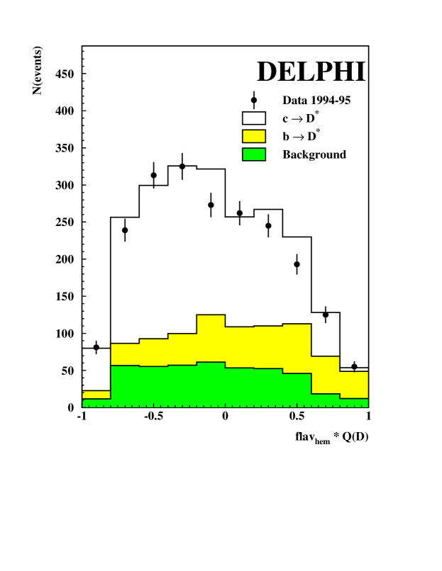
Figure 11: The product of the charge tagging Neural Network output times the charge of a reconstructed ${\mathrm{D}}^{*}$ in the opposite hemisphere. Only a subset of the full samples is shown here for illustration purposes: The data comprise the four decay channels ${{\mathrm{D}}^{*+}\to(X)\pi^{+}}$, where $X$ can be $K^{-}\pi^{+}$, $K^{-}\pi^{+}\gamma\gamma$, $K^{-}\pi^{+}\pi^{-}\pi^{+}$ or $K^{-}\pi^{+}(\pi^{0})$, for the years 1994-95. The $c\to{\mathrm{D}}^{*}$ fraction was increased by requiring $X_{E}>0.45$ and the event ${b\mbox{-}tag}$ in the range $-0.7$ to $1.0$. The b-quark and combinatorial background is corrected using the measured distribution from a c-depleted selection on the same data samples.

To separate the contributions from c and b events on the data themselves, a two dimensional fit was performed using the D energy and the b tagging information in the D hemisphere as separating variables. The latter avoids a possible correlation between the hemisphere b tagging and the hemisphere charge tagging in the hemisphere opposite to the ${\mathrm{D}}$ in which $w_{c}$ is to be measured. To make a sensitive measurement, the analysis to determine the c-quark charge tagging probability is performed on the full set of 9 different exclusive D decay modes used by DELPHI to measure the charm asymmetry [16]. In addition, the requirements for a charge tag as used in the rest of this paper were slightly modified, in that the b-tag cut was relaxed to ${b\mbox{-}tag}{}>-0.7$ for the purpose of preserving enough charm events in the fitted sample. It has been checked that there is no significant change in $w_{c}$ while moving the b-tag working point from ${p_{{\mathrm{b}}}}=90\,\%$ to a ${p_{{\mathrm{b}}}}$ of about $75\,\%$. Combining the individual results from all nine decay modes and all four years 1992-95, the charm charge tagging probability was found to be different from the simulated one by a factor $0.944\pm 0.030$ as shown in Figure 12. This means that charm charge tagging is in fact weaker than predicted in simulation.

In the fit to $A_{FB}^{{\mathrm{b}}}$, Equations 15 and 16, $w_{{\mathrm{c}}}$ enters via the dilution factor $2w_{c}-1$. The simulated dilution factor is then scaled by the data to simulation ratio obtained for $2w_{c}-1$ from the set of reconstructed D events, namely $0.71\pm 0.15$.

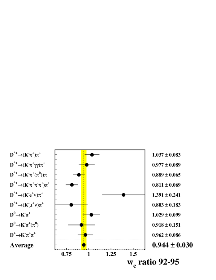
Figure 12: The ratio of real data to simulation in the c-quark charge identification $w_{c}$ provided by a ${flav_{\mbox{\tiny hem}}}$ tag in a hemisphere opposite a reconstructed D. The final result is decomposed into the 9 different decay channels used in [16].

6 The measurement of $A_{FB}^{{\mathrm{b}}}$

The differential asymmetry is insensitive to changes in the detector efficiency between different bins in polar angle. Hence the measurement of the b asymmetry is done in consecutive intervals of $\cos\theta_{\vec{T}}$. According to the different VD set-ups, eight equidistant bins covering $\cos\theta_{\vec{T}}\in[0.0,0.825]$ are chosen for 1992 and 1993, and nine bins covering $\cos\theta_{\vec{T}}\in[0.0,0.925]$ for 1994 to 2000. In each bin the observed asymmetry is given by replacing the forward-backward asymmetry $A_{FB}^{{\mathrm{f}}}$ in Equations 15 and 16 by the differential asymmetry:

$$\mbox{\begin{math}A_{FB}^{{\mathrm{f,diff}}}\end{math}}(\cos{\theta_{\vec{T}}}) = \frac{8}{3}\cdot A_{FB}^{{\mathrm{f}}}\cdot\frac{\cos{\theta}}{1+\cos^{2}{\theta}}~{}.$$ (25)

To extract $A_{FB}^{{\mathrm{b}}}$ all parameters of Equations 15 and 16 need to be determined bin by bin. The flavour fractions were calculated from the data in Section 5.3. The probabilities $w_{{\mathrm{b}}}$ and $w_{{\mathrm{b}}}^{D}$ to identify the b-quark charge correctly as a function of the polar angle were discussed in Section 5.4. This includes corrections for the hemisphere correlations for each bin. The c-quark backgound $w_{{\mathrm{c}}}^{(D)}$ is calibrated by means of exclusively reconstructed D hemispheres described in Section 5.6. The probability of identifying the quark charge on the small amount of light quark background is estimated from simulation using Equation 17 for the single tagged and Equation 18 for the double tagged events.

The background forward-backward asymmetries for d-, u- and s-quark events are set to the Standard Model values, and for c vents the forward-backward asymmetry is set to its measured LEP value ($A_{FB}^{{\mathrm{c}}}(91.260\,\mbox{GeV})\,=\,0.0641\pm 0.0036$). It is extrapolated by means of Zfitter to the DELPHI centre-of-mass energies, giving -0.0338, 0.0627 and 0.1241 for peak-2, peak and peak+2 [12, 15].

6.1 The QCD correction

The measurement of the b-quark forward-backward asymmetry is sensitive to QCD corrections to the quark final state. The correction takes into account gluon radiation from the primary quark pair and the approximation of the initial quark direction by the experimentally measured thrust axis. The effects of gluon radiation have been calculated to second order in $\alpha_{s}$ for massless quarks, and for an asymmetry based on the parton level thrust axis. The remaining correction from the parton to the hadron level thrust axis has been determined by means of hadronisation models in Monte Carlo simulation.

A realistic measurement has a reduced experimental sensitivity to the QCD effects because of biases in the analysis against events with hard gluon radiation. In this analysis the charge tagging and also the b tagging introduce a bias against QCD effects. Therefore the QCD correction can be written as [17]:

$$\mbox{\begin{math}\kern 0.84009ptA_{FB}^{{\mathrm{b}},QCD}\,\end{math}}=(1-C_{{\mathrm{b}}})\kern 0.84009ptA_{FB}^{{\mathrm{b}},noQCD}\,=(1-s_{{\mathrm{b}}}\,C^{{\mathrm{b}}}_{QCD})\kern 0.84009ptA_{FB}^{{\mathrm{b}},noQCD}\,.$$ (26)

Here $\kern 0.84009ptA_{FB}^{{\mathrm{b}},noQCD}\,$ is the asymmetry of the initial b-quarks without gluon radiation, which can be calculated from the measured asymmetry $\kern 0.84009ptA_{FB}^{{\mathrm{b}},QCD}\,$ through the correction coefficient $C_{{\mathrm{b}}}$. This correction coefficient can be decomposed into a product of the full QCD correction $C^{{\mathrm{b}}}_{QCD}$ to the b-quark asymmetry measured using the thrust direction and the sensitivity $s_{{\mathrm{b}}}$ of the individual analysis to $C^{{\mathrm{b}}}_{QCD}$.

The experimental bias is studied on simulation by fitting the differential asymmetry of the b simulation after setting the generated asymmetry of the initial b-quarks before gluon radiation to the maximum of $75\,\%$ (Eq. 25). The observed relative differences of the asymmetries are studied separately for each $\cos\theta_{\vec{T}}$ interval and bin in b-tag. In Figure 13 the coefficient $C_{{\mathrm{b}}}$ is shown for single and double tagged events for the different years. At small $\cos\theta_{\vec{T}}$ values the sensitivity to the asymmetry is small and hence $C_{{\mathrm{b}}}$ receives a larger statistical uncertainty. Note that no systematic variation of $C_{{\mathrm{b}}}$ with $\cos\theta_{\vec{T}}$ is seen at large polar angles. From the coefficient $C_{{\mathrm{b}}}$ the experimental bias factor $s_{{\mathrm{b}}}$ is deduced, using a value [17] of $C^{{\mathrm{b}},\,\mathrm{sim.}}_{QCD}=(3.06\pm 0.03)\%$ that is specific to the physics and detector modelling in the DELPHI simulation. The values of $s_{{\mathrm{b}}}$ averaged over bins in ${b\mbox{-}tag}$ and polar angle are shown in Table 4 for the different years of data taking.

year	$s_{{\mathrm{b}}}$ [$\%$]
1992	27$\pm$	7
1993	21$\pm$	8
1994	13$\pm$	5
1995	13$\pm$	9
1996-2000	14$\pm$	9

Table 4: Summary of bias factors $s_{{\mathrm{b}}}$ with their statistical uncertainty.

On real data the theoretical calculation discussed above is applied, as the calculation is expected to be more reliable than the simulation. The correction factor has been updated in reference [18], giving $C^{{\mathrm{b}},\,\mathrm{est.}}_{QCD}=(3.54\pm 0.63)\%$. In the following fits the correction coefficients $s_{{\mathrm{b}}}\cdot{}C^{{\mathrm{b}},\,\mathrm{est.}}_{QCD}$ are taken into account for each bin in polar angle separately and hence all asymmetries quoted are corrected for QCD effects.

Figure 13: The size of the QCD correction including experimental biases as a function of the polar angle of the thrust axis. In the upper plot the correction is shown for single charge tagged events from the different years. In the lower plot the corresponding corrections are shown for double charge tagged events.

6.2 The fit of the b-quark forward-backward asymmetry

The b-quark forward-backward asymmetry is extracted from a $\chi^{2}$-fit dividing the data of each year in 4 intervals of b-tag. This allows for the change in b purity (Table 5.3) and in the size of the hemisphere correlations as a function of b-tag. In addition, it reduces the dependence on the charm asymmetry from $\pm 0.00023$ for a single cut on b-tag to the value of $\pm 0.00014$ which is found in the present analysis. Technically $A_{FB}^{{\mathrm{b}}}$ is extracted in each interval from a $\chi^{2}$-fit to the five independent event categories $N$, $\overline{N}$, $N^{D}$, $\overline{N^{D}}$and $N^{same}$  in bins of polar angle.

The double charge tagged unlike-sign events are sensitive to the asymmetry, but the rates also enter into the determination of the charge tagging probabilities $w_{{\mathrm{b}}}$ and $w_{{\mathrm{b}}}^{D}$, as can be seen in Equations 23 and 24. This leads to correlations between the probabilities and the measured asymmetry in each bin. In the combined $\chi^{2}$-fit to the five event rates $N$, $\overline{N}$, $N^{D}$, $\overline{N^{D}}$ and $N^{same}$  these correlations are taken into account. Using the equations above, the rates can be expressed as a function of the b-quark forward-backward asymmetry $A_{FB}^{{\mathrm{b}}}$, the probability $w_{{\mathrm{b}}}$ and two arbitrary normalisation factors which absorb the overall efficiency corrections. These normalisations are set to their proper values for each bin in the fit. The number of degrees of freedom $(ndf)$ is 15 for 1992+93 and 17 for 1994-2000. The $\chi^{2}$ probabilities for the 36 fits in the different intervals in b-tag, years and energy points have been verified, and an average $\chi^{2}/ndf$ of 1.07 was found with an r.m.s. of 0.38. It has been cross-checked on simulation that the fitted forward-backward asymmetry $A_{FB}^{{\mathrm{b}}}$ reproduces the true forward-backward asymmetry $A_{FB}^{{\mathrm{b}}}$ of the simulated b-quark events. The statistical precision with which the true asymmetry is refound in the analysis is $\pm 0.0017$. Another check has studied directly a possible statistical bias depending on the size of the samples in the double tagging technique. The effect of such a bias on this analysis was found to be negligible.

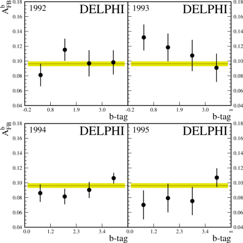
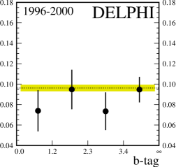
Figure 14: The $A_{FB}^{{\mathrm{b}}}$  results for each year and each interval in b-tag with their statistical errors. The 20 individual measurements enter into the final fit taking into account statistical and systematic errors. The line is the average from the $\chi^{2}$-fit at $\sqrt{s}=91.231$ GeV with its statistical uncertainty shown as the band.

In Figure 14 the measured asymmetries with their statistical errors are shown in intervals of b-tag for the different years. The band represents the overall result $A_{FB}^{{\mathrm{b}}}(91.231\,\mbox{GeV})\,=\,{0.0958}\pm{0.0032}(\mbox{stat.})$ with its statistical uncertainty. Figure 15 shows the measured differential asymmetry for single and double tagged events as a function of $\cos\theta_{\vec{T}}$ averaged over all years of data taking and over all b-tag intervals. Again, only statistical uncertainties are shown and the band represents the overall result.

6.2.1 The off-peak data sets

The data sets at 2 GeV above and below the Z-pole each have about a factor five less events than the corresponding on-peak data. They are analysed using the same method as the $91.231$ GeV data, but with a few adaptations:

• For the off-peak data taken intermittently between the Z peak running, no extra ${\varepsilon_{\mathrm{b}}}$/${\varepsilon_{\mathrm{c}}}$ calibration was carried out, but the peak correction functions were applied.

• The energy dependence of the charge tagging performance is negligible over this small range of centre-of-mass energies. So the peak quantities related to the charge tagging for the two years in question are transferred to the off-peak analysis. These quantities are the $w_{{\mathrm{b}}}$ and $w_{{\mathrm{c}}}$ measurements on data as well as the simulated charge tagging input to the fit, $w_{\mathrm{uds}}$, the correlations $\delta$ and $\beta$ and the QCD correction $C_{b}$.

• The number of $\cos\theta_{\vec{T}}$ bins is reduced. For 1993 from 8 to 4 and for 1995 from 9 to 5, always covering the same range. The corresponding $\chi^{2}$-fits to the event numbers have 11 degrees of freedom for 1993 and 14 for 1995.

Figure 16 shows the results in intervals of b-tag separated for each year.

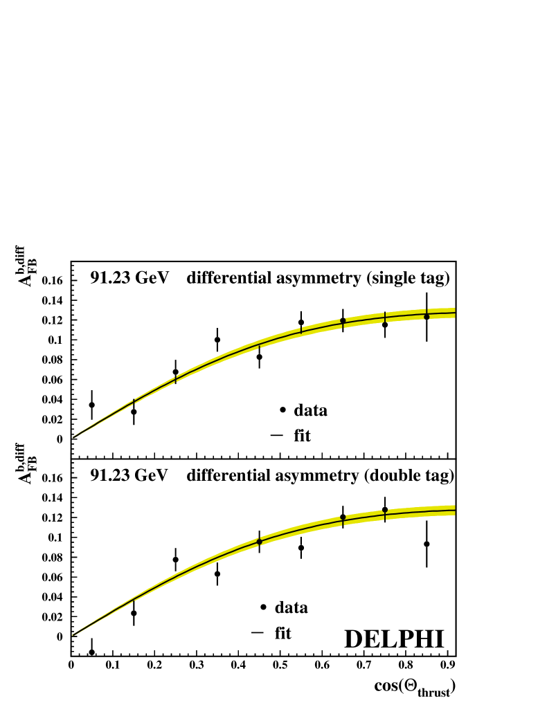
Figure 15: The differential b-quark forward-backward asymmetry of the years 1992 to 2000 at a centre-of-mass energy of 91.231 GeV. It is shown separately for the two classes of single and double charge tagged events. The curve is the result of the common $\chi^{2}$-fit with its statistical error shown as the band.

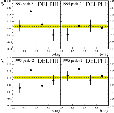
Figure 16: The $A_{FB}^{{\mathrm{b}}}$  results for the 1993 and 1995 off-peak runs and each interval in b-tag with their statistical errors. The lines in the upper and lower plots are the results of $\chi^{2}$-fits that were run separately at $\sqrt{s}=89.449$ and $92.990$ GeV. The band shows again the statistical uncertainty.

Year	$\sqrt{s}$ [GeV]	$A_{FB}^{{\mathrm{b}}}$	prob$(\chi^{2})$
1992	91.280	0.0984 $\pm$ 0.0079	0.47
1993	91.225	0.1130 $\pm$ 0.0095	0.46
1994	91.202	0.0952 $\pm$ 0.0048	0.19
1995	91.288	0.0895 $\pm$ 0.0084	0.30
1996-2000	91.260	0.0870 $\pm$ 0.0083	0.69
1993 peak-2	89.431	0.0803 $\pm$ 0.0216	0.05
1993 peak+2	93.015	0.0817 $\pm$ 0.0177	0.06
1995 peak-2	89.468	0.0506 $\pm$ 0.0191	0.71
1995 peak+2	92.965	0.1213 $\pm$ 0.0152	0.40

Table 5: Summary of the $A_{FB}^{{\mathrm{b}}}$  results for the different years with their statistical uncertainty. Systematic errors, as to be discussed in Section 7, and statistical errors are taken into account when combining the different b purity samples. The number of degrees of freedom is $(4-1)$ for the fit of each year of data taking. The prob($\chi^{2}$) denotes the probability to find the observed agreement (or worse) with each result.

6.2.2 Combined results

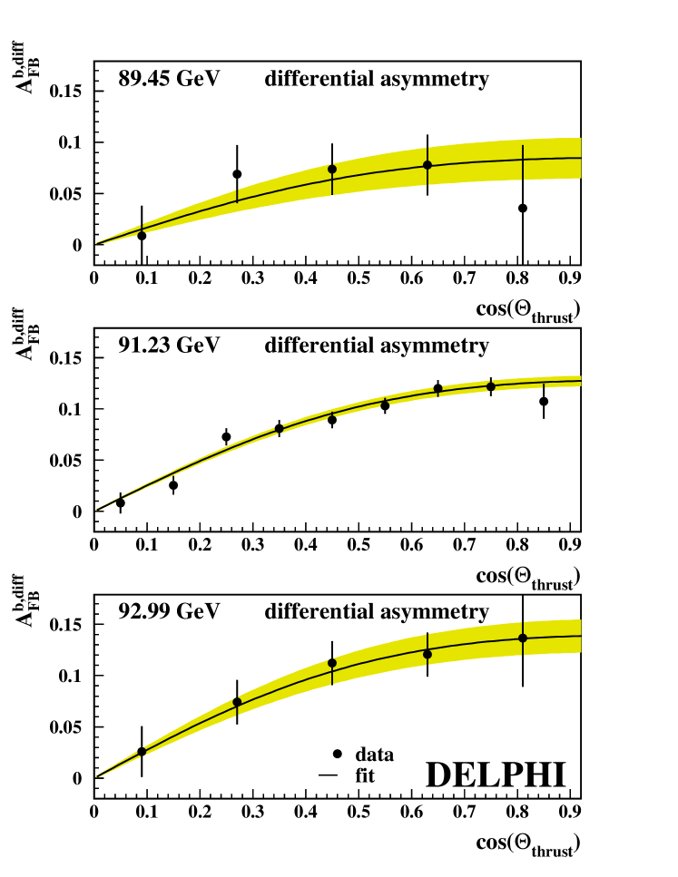
Figure 17: The differential b-quark forward-backward asymmetry (single and double tag) at the three centre-of-mass energies of 91.231, 89.449 and 92.990 GeV. The curve is the result of the common $\chi^{2}$-fit with its statistical error shown as the band.

The summary of the individual $A_{FB}^{{\mathrm{b}}}$ results for the different years with their statistical uncertainties is given in Table 5. Combining these measurements taking common uncertainties into account yields the final result:

$A_{FB}^{{\mathrm{b}}}$(89.449 GeV)	=	${0.0637}\pm{0.0143}(\mbox{stat.})$ ,
$A_{FB}^{{\mathrm{b}}}$(91.231 GeV)	=	${0.0958}\pm{0.0032}(\mbox{stat.})$ ,
$A_{FB}^{{\mathrm{b}}}$(92.990 GeV)	=	${0.1041}\pm{0.0115}(\mbox{stat.})$ .

The measured differential asymmetry in Figure 17 displays these averaged results from all three centre-of-mass energies, combining single and double tagged events.

7 Discussion of systematic uncertainties

The two main components of the analysis are the enhanced impact parameter b tagging and the Neural Network charge tagging. Both components are sensitive to detector resolution effects as well as to the modelling of light quark and c events in the simulation. Therefore both careful tuning of the simulation and measuring all possible input parameters directly have been applied as described above. Remaining uncertainties are studied and changes in the result are propagated through the whole analysis chain. The variation of systematic errors as a function of the b-tag intervals is taken into account.

The sources of systematic uncertainty affecting this measurement are discussed in the following sections. Their corresponding contributions to the systematic error are summarised in Tables 6 and 7.

Dependencies on the electroweak parameters

The LEP+SLD average values [12] for the electroweak parameters $R_{{\mathrm{b}}}^{0}=0.21644\pm 0.00065$, $R_{{\mathrm{c}}}^{0}=0.1719\pm 0.0031$ and $A_{FB}^{{\mathrm{c}}}=0.0641\pm 0.0036$ are used. They enter the determination of the b-tag correction function and the flavour fractions in the selected data sets, and they form the main background asymmetry in the measurement. Variations of $\pm 1\sigma$ with respect to the LEP+SLD averages are included in the systematic error.

Detector resolution

The detector resolution on the measured impact parameter affects both the b tagging and the charge tagging in a similar fashion, because both tagging algorithms exploit the lifetime information in the events. A poor description of the resolution in the simulation may lead to an erroneous estimation of remaining background in the sample. In the analysis a careful year by year tuning of these resolutions and of the vertex detector efficiency has been used [10] for both tagging packages.

For the systematic error estimation the recipe from the DELPHI $R_{b}$ measurement [11] was followed. First the calibration of the impact parameter significance for the simulation was replaced by the corresponding one for the real data to test residual differences between data and simulation. Second the VD efficiency correction was removed from the simulation. Finally the resolution of the impact parameter distribution was changed by $\pm 1\sigma$ with respect to the measured resolution in a real data sample depleted in b events. For every change the b tagging correction functions used to calibrate ${\varepsilon_{\mathrm{c}}}$ and ${\varepsilon_{\mathrm{b}}}$ have been re-calculated, and their effect has been propagated through the full analysis. Thus the detector description variation affects both b and charge tagging in a consistent way. The systematic uncertainty quoted was chosen conservatively as the linear sum of all three contributions, for which the last one gives the dominant uncertainty.

Hemisphere $b$-$tag$ correlations and calibration of the charm background

The efficiency for tagging charm in the b tagging procedure enters the background subtraction via the flavour fractions. The double tagging technique described in Section 4.2 measures the charm efficiency directly on the data while taking the uds efficiency and the b tagging correlations from simulation. This leads to a residual uncertainty on the charm efficiency which is estimated from a set of correction functions with varied simulation inputs. The uds efficiency is closely related to the detector resolution of which the consistent variation has already been discussed.

The b tagging hemisphere correlations $k_{j}$ were measured in the DELPHI $R_{b}$ measurement [11] and their uncertainties studied in detail. It was found that angular effects, gluon radiation and to a lesser extent also B physics modelling had a total effect of $\pm 20\,\%$ on the correlation. In this analysis the correlations $k_{j}$ were varied by $\pm 20\,\%$ and the effect of this variation on the calculated flavour efficiencies and fractions was propagated through the $A_{FB}^{{\mathrm{b}}}$ analysis.

The calibration functions that are applied to simulated charm events in the barrel and forward regions are displayed in Figure 18 for the working point correction and for the re-calculated correction with varied correlations, varied detector resolution and varied LEP/SLD inputs. Different detector conditions in the years 1992+93 and 1994+95 as well as the barrel and forward range result in different correction functions. At low b-tag${}_{\mbox{\tiny hem}}$ values where charm is an important background, the variation of the resolution modelling has the largest impact on the calibration correction. At higher b-tag${}_{\mbox{\tiny hem}}$ values the variation of the b tagging hemisphere correlation becomes dominant. However there the charm background is already so much reduced that the total impact on the analysis remains low, leading to a small contribution to the systematic uncertainty on $A_{FB}^{{\mathrm{b}}}$.

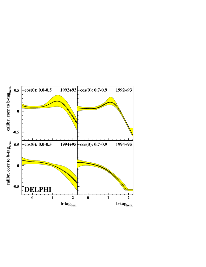
Figure 18: The values of the c efficiency correction function applied to the b-tag${}_{\mbox{\tiny hem}}$ variable on simulated c events. They are shown for the two most important year periods and for events in the central and forward regions of the detector. For each systematic variation that affects the b tagging calibration the functions were re-calculated, leading to slightly shifted shapes. The maximal and minimal correction found for any variation span the error band, namely the resolution variation at b-tag${}_{\mbox{\tiny hem}}$ below 0.5 and the correlation variation elsewhere.

Charge identification for b-quarks

The b-quark charge identification probability is measured directly from data using the double tagging technique described above. Small correlations between the charge identification probability in each $\cos\theta_{\vec{T}}$ bin and $A_{FB}^{{\mathrm{b}}}$ via the double tagged opposite sign events are therefore automatically taken into account. The statistical uncertainties of the charge identification probabilities $w_{{\mathrm{b}}}$ and $w_{{\mathrm{b}}}^{D}$ are determined in the $\chi^{2}$-fit and are included in the statistical error on $A_{FB}^{{\mathrm{b}}}$.

Charge identification for background

The charge separation for the background of charm events determines directly the background asymmetry correction, which itself enters with opposite sign. Events with exclusively reconstructed D mesons have been used in Section 5.6 to correct the simulated $w_{{\mathrm{c}}}^{(D)}$ on the data. The statistical uncertainty on the scaling factor to $(2w_{{\mathrm{c}}}\!-\!1)$, $0.71\pm 0.15$, from the measurement based on the exclusively reconstructed D mesons is used to determine the uncertainty on $w_{c}$ in the asymmetry measurement.

The Neural Network charge tag is sensitive to the details of vertexing in uds events. From the distributions of the Network inputs and the $flav_{\mbox{\tiny hem}}$ output variable at different b purities there is no indication that the light quark charge tagging is not correctly simulated. Nevertheless the full uds correction is chosen as a conservative error.

Hemisphere charge correlations

The charge tagging hemisphere correlations are an important source of systematic uncertainty. The hemisphere charge correlations $\delta$ and $\beta$ for this measurement are introduced by the jet charge as discussed in Section 5.5. In reference [2] the hemisphere correlation for the jet charge at different values of $\kappa$ has been measured from the data. Comparing the result to the simulation, an uncertainty of $\pm 20\,\%$ was assigned to the $\delta$ and $\beta$. It was checked that the use of $\cos\theta_{\vec{T}}$ dependent correlations compared to a constant average value has no effect on the analysis.

For the measurement discussed here the size of the hemisphere correlation is given by the relative weight of the jet charge and the vertex based charge information. This variation is explicitly allowed for using intervals in b-tag, as for high values of b-tag good vertexing information is present in the event and consequently the hemisphere correlations are small. The correlations $\delta$ and $\beta$ as a function of the b-tag interval are shown as the full dots in Figure 19.

  

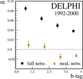
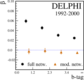
Figure 19: The charge hemisphere correlations for the on-peak data of 1992-2000 versus the interval in b-tag. The results using the full hemisphere charge tag (full dots) are compared to a modified version of the Neural Network (triangles) in which the jet charge with $\kappa=0.3$ was taken out.

As already mentioned before, the correlations arise mainly from charge conservation in the event and are introduced into the analysis mainly via the jet charge at $\kappa=0.3$, which is sensitive to tracks with low momenta. The possibility used in Figure 10 to remove the jet charge from the inputs to the Neural Network has also been exploited to test the stability of the central value directly. Figure 19 displays the mean hemisphere correlations versus the intervals in b-tag once for the full Neural Network as used throughout the analysis and once for the modified Network (full triangles) with $Q_{J}(\kappa=0.3)$ taken out. For the modified Neural Network the correlations are close to zero.

When using the modified hemisphere charge Network, the $A_{FB}^{{\mathrm{b}}}(91.231\,\mathrm{GeV})$ result shifts by $+0.0011$. This is $0.6\sigma$ of the expected statistical uncertainty comparing the data samples selected by the modified and the full charge tag. The shift corresponds to $+1\sigma$ in the systematic error quoted for the $\pm 20\,\%$ uncertainty related to the hemisphere correlation.

Gluon splitting

In light quark events a gluon splitting into a $\mbox{c}\overline{\mbox{c}}$ pair or $\mbox{b}\overline{\mbox{b}}$ pair gives rise to lifetime information from the decays of the produced heavy quark hadrons. A variation of the splitting rates within the errors on the present world averages $g\to\mbox{c}\overline{\mbox{c}}=(2.96\pm 0.38)\,\%$ and $g\to\mbox{b}\overline{\mbox{b}}=(0.254\pm 0.051)\,\%$ [19] is included in the systematic error.

Rate of $K^{0}$ and $\Lambda$

Decays of K⁰ and $\Lambda$ in flight lead to tracks with large impact parameters with respect to the primary vertex and consequently can lead to a lifetime information in light quark events. The rate of such decays in light quark events was varied by $\pm 10\%$ to estimate the effect on the light quark efficiency $\epsilon_{\mathrm{uds}}$ .

QCD correction and QCD experimental bias

The size of the QCD correction is theoretically known to be $0.0354\pm 0.0063$ [18]. The experimental bias of the full analysis on the QCD correction has been discussed in Section 6.1. Therefore the systematic uncertainty due to the QCD correction receives two contributions, one given by the statistical precision with which the QCD bias was estimated on simulation, the other one is given by the theoretical error multiplied by the experimental bias.

In Figure 10 the hemisphere correlations $\beta$ and $\delta$ are shown with and without applying a cut of $\mathrm{thrust}>0.9$. The differences are due to effects from gluon radiation. Hence the correction for the hemisphere correlations includes an implicit QCD correction. From the variation of the hemisphere correlation as a function of the thrust cut the bias on the QCD correction from hemisphere correlations is estimated to be $50\,\%$. This additional bias factor has to be taken into account for the systematic error due to the theoretical uncertainty, adding $0.00031$ to the value obtained from the study that uses only the simulated QCD bias.

Statistical error of simulation

The contribution to the total error due the limited size of the simulated sample can be estimated by dropping from the $\chi^{2}$-fit the statistical uncertainties from the simulation. It is quoted separately from the pure statistical error of the data.

Contribution	Variation	$\Delta A_{FB}^{{\mathrm{b}}}\times 10^{2}$
		$\sqrt{s}=89.449$	$\sqrt{s}=91.231$	$\sqrt{s}=92.990$
$R_{{\mathrm{b}}}^{0}$	$0.21644\pm 0.00065$	$\mp 0.010$	$\mp 0.011$	$\mp 0.016$
$R_{{\mathrm{c}}}^{0}$	$0.1719\pm 0.0031$	$\mp 0.010$	$\mp 0.014$	$\mp 0.021$
$A_{FB}^{{\mathrm{c}}}$	$0.0641\pm 0.0036$	$\pm 0.019$	$\pm 0.014$	$\pm 0.018$

Table 6: Dependencies of $A_{FB}^{{\mathrm{b}}}$ on the electroweak parameters. The effect of the $\pm 1\sigma$ variation contributes to the systematic uncertainty. The measured value of $A_{FB}^{{\mathrm{c}}}$ from [12] is extrapolated to DELPHI centre-of-mass energies by means of Zfitter, giving -0.0338, 0.0627 and 0.1241 for peak-2, peak and peak+2.

Contribution	Variation	$\Delta A_{FB}^{{\mathrm{b}}}\times 10^{2}$
		1992-2000
detector resolution	see text	$\pm 0.035$
hemisphere b-tag correlations	$\pm 20\,\%$	$\pm 0.011$
c charge separation	see text	$\pm 0.025$
uds charge identification	full effect	$\mp 0.048$
hemisphere charge correlations	$\pm 20\,\%$	$\pm 0.107$
gluon splitting $g\to b\bar{b}$	$0.00235\pm 0.00051$	$\pm 0.005$
gluon splitting $g\to c\bar{c}$	$0.0296\pm 0.0038$	$<0.0001$
rate of $K^{0}/\Lambda$	$\pm 10\,\%$	$\pm 0.006$
error on QCD bias	see text	$\pm 0.022$
uncertainty of QCD correction	see text	$\pm 0.040$
statistical error of simulation		$\pm 0.016$
total systematic error		$\pm 0.14$

Table 7: Systematic uncertainties and their influence on the determination of $A_{FB}^{{\mathrm{b}}}$.

7.1 Additional tests

The fit to $A_{FB}^{{\mathrm{b}}}$ is performed in four intervals in b-tag with averaged b purities ranging from $74\,\%$ up to $99.7\,\%$. This takes into account a correlation between b and charge tagging by permitting a purity dependence in quantities related to the latter, such as $w_{{\mathrm{b}}}^{(D)}$ and $\delta$, $\beta$. Furthermore, a varying dependence on detector modelling, residual backgrounds and the hemisphere charge correlations (see Fig. 19) leads to a systematic error that decreases with increasing purity. Fig. 20 illustrates the stability of the 1992-2000 combined $A_{FB}^{{\mathrm{b}}}$ measurement as a function of b purity.

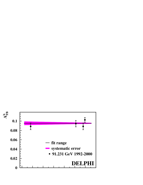
Figure 20: The peak asymmetry for the combined years 1992-2000 obtained on event samples with different b purity. The data points are the results from Figure 14 in comparison with the 1992-2000 fit result (line). The band shows the systematic error as a function of the b purity. The lower plot illustrates how the background is composed of c and light quarks events.

Figure 21: The b-quark pole asymmetry for different cuts on the thrust value. It is compared to the final result from all three centre-of-mass energies which does not use any thrust cut (left hand side). The small error bars with the serifs show the uncorrelated statistical error estimated from the quadratic difference of the correlated errors.

The QCD correction and light quark fragmentation modelling are the dominant systematic uncertainties in the LEP average $A_{FB}^{{\mathrm{b}}}$ results [12]. Also this measurement is subject to gluon radiation entering via the hemisphere correlations and the sensitivity to the QCD correction. To test if this is correctly taken into account a cut on the thrust variable $T$ was introduced and the full analysis was repeated with different settings of the cut value. The full data-set of 1992 to 2000 at all three centre-of-mass energies was used to make the test as sensitive as possible. The results of this check are displayed in Figure 21 with both correlated and uncorrelated statistical errors. No dependency on the thrust cut is found.

Figure 22: The asymmetry between double positive and double negative tagged events illustrates the charge bias observed in this analysis. The effect is less distinct in the real data.

Another study covered the positive charge bias that is introduced by the presence of hadronic interactions with matter in the detector. In this analysis the sample of double like-sign events was split up into events with both hemispheres tagged positive, $N_{++}$ , and both negative, $N_{--}$ . A charge asymmetry

$${A_{++--}^{\mathrm{obs.}}}=\frac{{N_{++}}-{N_{--}}}{{N_{++}}+{N_{--}}}$$ (27)

was then formed which is displayed in Figure 22 versus the bin in $\cos\theta_{\vec{T}}$ for the sum of all peak data-sets. Although tracks from secondary interactions are suppressed by both DELPHI track reconstruction and the analysis package for b physics, a residual charge bias can be seen. In simulation the charge bias is found to be significantly larger than in the real data. No dependence on $\cos\theta_{\vec{T}}$ was observed. Being constructed as the difference of two charges or count rates, the asymmetry is not sensitive to such a charge bias, as was verified on simulation.

8 Conclusions

This measurement of $A_{FB}^{{\mathrm{b}}}$ uses an enhanced impact parameter b tagging and an inclusive b-quark charge tagging Neural Network. The analysis is based on the LEP 1 data collected with the DELPHI detector from 1992 up to 1995 and the LEP 2 calibration runs at the Z pole from 1996 to 2000. The measured b-quark forward-backward asymmetries for the individual years of data taking are:

year	$\sqrt{s}$ [GeV]	$A_{FB}^{{\mathrm{b}}}$ ($\pm$ stat.$\pm$syst.)
1992	91.280	0.0984  $\pm$ 0.0079$\pm$ 0.0018
1993 peak-2	89.431	0.0803 $\pm$ 0.0216$\pm$ 0.0022
1993	91.225	0.1130  $\pm$ 0.0095$\pm$ 0.0021
1993 peak+2	93.015	0.0817 $\pm$ 0.0177$\pm$ 0.0021
1994	91.202	0.0952  $\pm$ 0.0048$\pm$ 0.0014
1995 peak-2	89.468	0.0506 $\pm$ 0.0191$\pm$ 0.0020
1995	91.288	0.0895  $\pm$ 0.0084$\pm$ 0.0020
1995 peak+2	92.965	0.1213 $\pm$ 0.0152$\pm$ 0.0035
1996-2000	91.260	0.0870  $\pm$ 0.0083$\pm$ 0.0018

These measurements include the QCD correction. The final result is obtained taking correlated systematic errors, mainly from QCD, into account:

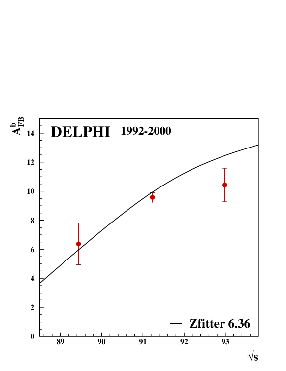
Figure 23: The $A_{FB}^{{\mathrm{b}}}$  results versus the centre-of-mass energy. The total errors (bars) are only slightly larger than the statistical (flags). The curve represents the Standard Model prediction obtained from Zfitter [15].

$A_{FB}^{{\mathrm{b}}}$(89.449 GeV)	=	${0.0637}\pm{0.0143}(\mbox{stat.})\pm{0.0017}(\mbox{syst.})$  ,
$A_{FB}^{{\mathrm{b}}}$(91.231 GeV)	=	${0.0958}\pm{0.0032}(\mbox{stat.})\pm{0.0014}(\mbox{syst.})$  ,
$A_{FB}^{{\mathrm{b}}}$(92.990 GeV)	=	${0.1041}\pm{0.0115}(\mbox{stat.})\pm{0.0024}(\mbox{syst.})$  .

These measurements are shown in Figure 23 together with the Zfitter calculation [15], and are in reasonable agreement with the Standard Model prediction.

From this measurement the Z pole b-quark asymmetry is extracted. Two corrections for QED: photon exchange and $\gamma$ Z interference amount to $+0.0039$ and $-0.0006$, respectively. A correction of $-0.0009$ is applied to correct for the energy dependence of the asymmetry. The corrections have been newly re-calculated in [20]. This yields:

$A_{FB}^{0,{\mathrm{b}}}$

=

${0.0982}\pm{0.0032}(\mbox{stat.})\pm{0.0014}(\mbox{syst.})$  .

Assuming a Standard Model like energy dependence the results from the two energy points above and below the Z peak can be included in the pole asymmetry:

$A_{FB}^{0,{\mathrm{b}}}$

=

${0.0972}\pm{0.0030}(\mbox{stat.})\pm{0.0014}(\mbox{syst.})$  .

Using equations 1 and 2 for the effective electroweak mixing angle ${\mathrm{sin}}^{2}\theta_{\mathrm{eff}}^{\ell}$ gives:

${\mathrm{sin}}^{2}\theta_{\mathrm{eff}}^{\ell}$

=

${0.23259}\pm{0.00054}$

The measurement presented in this paper agrees well with previous determinations of $A_{FB}^{0,{\mathrm{b}}}$ at LEP and consequently with the current LEP average value of $A_{FB}^{0,{\mathrm{b}}}=0.0992\pm 0.0017$ [2, 3, 21, 22]. It improves on the precision with respect to the previous DELPHI results by a factor of $1.36$.

9 The DELPHI combined results for $A_{FB}^{0,{\mathrm{b}}}$ and $A_{FB}^{0,{\mathrm{c}}}$

Precision measurements of the b-quark forward-backward asymmetry are obtained in DELPHI from three independent methods, differing mainly in the way the b charge is reconstructed. They are based on the lepton charge in semileptonic B decays [3], on the jet charge [2] in b tagged events or on the Neural Network charge tag in the analysis presented here. The results for all three measurements are compared in Table 8, showing a good mutual agreement.

Method	data sets	$A_{FB}^{0,{\mathrm{b}}}$
lepton charge	1991-95	$0.1015\pm 0.0052\pm 0.0024$
jet charge	1992-95	$0.1006\pm 0.0044\pm 0.0015$
Neural Network	1992-2000	${0.0972}\pm{0.0030}\pm{0.0014}$

Table 8: Results from the three most precise $A_{FB}^{{\mathrm{b}}}$ measurements performed on the DELPHI data at the three centre-of-mass energies $89.449$, $91.231$ and $92.990$ GeV. From the published $A_{FB}^{0,{\mathrm{b}}}$ values for “lepton charge” and “jet charge” 0.0006 has been subtracted to comply with the corrections given in [20].

The measurements analyse common data sets and employ similar basic techniques, such as the b tagging and the jet charge. Hence there are statistical correlations between the three analyses that have been evaluated by monitoring common fluctuations on the large 1994 simulated data set, that was divided into 100 sub-samples for that purpose. The resulting values for the correlation are summarised in Table 9.

	$A_{FB}^{{\mathrm{b}}}$ NN	$A_{FB}^{{\mathrm{b}}}$ lepton
$A_{FB}^{{\mathrm{b}}}$ NN	1	$0.29\pm 0.09$
$A_{FB}^{{\mathrm{b}}}$ jet-ch.	$0.53\pm 0.07$	$0.31\pm 0.09$

Table 9: Correlations between the different methods used in DELPHI to determine the b asymmetry.

The analysis by means of the lepton charge in semileptonic B and D decays involves a correlation to charm. Therefore the combined DELPHI results for the b and c asymmetries are determined simultaneously, taking into account these statistical correlations as well as correlated systematic errors. The c and b asymmetry measurements from exclusively reconstructed D mesons [16] are also included in the combination. This combination gives the following values and their total errors

$$A_{FB}^{0,{\mathrm{b}}}=0.0984\pm 0.0029,\qquad A_{FB}^{0,{\mathrm{c}}}=0.0708\pm 0.0068$$

with a $\chi^{2}$/ndf of $11.2/(21-2)$ and a total correlation of $-0.050$ between them.

Acknowledgements

We are greatly indebted to our technical collaborators, to the members of the CERN-SL Division for the excellent performance of the LEP collider, and to the funding agencies for their support in building and operating the DELPHI detector.
We acknowledge in particular the support of
Austrian Federal Ministry of Education, Science and Culture, GZ 616.364/2-III/2a/98,
FNRS–FWO, Flanders Institute to encourage scientific and technological research in the industry (IWT), Belgium,
FINEP, CNPq, CAPES, FUJB and FAPERJ, Brazil,
Czech Ministry of Industry and Trade, GA CR 202/99/1362,
Commission of the European Communities (DG XII),
Direction des Sciences de la Mati$\grave{\mbox{\rm e}}$re, CEA, France,
Bundesministerium f$\ddot{\mbox{\rm u}}$r Bildung, Wissenschaft, Forschung und Technologie, Germany,
General Secretariat for Research and Technology, Greece,
National Science Foundation (NWO) and Foundation for Research on Matter (FOM), The Netherlands,
Norwegian Research Council,
State Committee for Scientific Research, Poland, SPUB-M/CERN/PO3/DZ296/2000, SPUB-M/CERN/PO3/DZ297/2000, 2P03B 104 19 and 2P03B 69 23(2002-2004)
FCT - Fundação para a Ciência e Tecnologia, Portugal,
Vedecka grantova agentura MS SR, Slovakia, Nr. 95/5195/134,
Ministry of Science and Technology of the Republic of Slovenia,
CICYT, Spain, AEN99-0950 and AEN99-0761,
The Swedish Natural Science Research Council,
Particle Physics and Astronomy Research Council, UK,
Department of Energy, USA, DE-FG02-01ER41155.
EEC RTN contract HPRN-CT-00292-2002.

Appendix A

In this measurement events are sorted into five different categories. These categories are defined in Section 2:

${N}$	$=$	number of single hemisphere tagged forward events,
${\overline{N}}$	$=$	number of single hemisphere tagged backward events,
${N^{D}}$	$=$	number of double hemisphere tagged forward events,
${\overline{N^{D}}}$	$=$	number of double hemisphere tagged backward events,
${N^{same}}$	$=$	number of double tagged like-sign events.

The probability to identify the quark charge correctly in single and double tagged events is specified by $w_{{\mathrm{f}}}$ and $w_{{\mathrm{f}}}^{D}$. For single tagged events the quantity is defined as:

$${w_{{\mathrm{f}}}}=\frac{{\hat{N}_{{\mathrm{f}}}}+{\hat{N}_{\overline{\mathrm{f}}}}}{{N_{{\mathrm{f}}}}+{N_{\overline{\mathrm{f}}}}}~{},$$ (28)

where ${N_{{\mathrm{f}}}}({N_{\overline{\mathrm{f}}}})$ is the number of events which contain a quark (anti-quark) in the forward hemisphere. ${\hat{N}_{{\mathrm{f}}}}({\hat{N}_{\overline{\mathrm{f}}}})$ is the number of events in which the quark (anti-quark) has been correctly identified.

For unlike-sign events the fraction of events in which both quark and anti-quark charges are correctly identified is defined analogously to the single hemisphere tagged events as the ratio of correctly tagged (${\hat{N}_{{\mathrm{f}}}^{D}},{\hat{N}_{\overline{\mathrm{f}}}^{D}}$) over all double-tagged unlike-sign (${N_{{\mathrm{f}}}^{D}},{N_{\overline{\mathrm{f}}}^{D}}$) events:

$${w_{{\mathrm{f}}}^{D}}=\frac{{\hat{N}_{{\mathrm{f}}}^{D}}+{\hat{N}_{\overline{\mathrm{f}}}^{D}}}{{N_{{\mathrm{f}}}^{D}}+{N_{\overline{\mathrm{f}}}^{D}}}~{}.$$ (29)

The single and double tagged unlike- and like-sign samples receive contributions from b events and from all other flavours. All categories also include events for which the quark charge was misidentified. Therefore the number of events entering in the different categories can be expressed as:

$${N} = \sum_{{\mathrm{f}}={\mathrm{d}},{\mathrm{s}},{\mathrm{b}}}\big{[}{N_{{\mathrm{f}}}}\cdot w_{{\mathrm{f}}}+{N_{\overline{\mathrm{f}}}}\cdot(1-w_{{\mathrm{f}}})\big{]}+\sum_{{\mathrm{f}}={\mathrm{u}},{\mathrm{c}}}\big{[}{N_{\overline{\mathrm{f}}}}\cdot w_{{\mathrm{f}}}+{N_{{\mathrm{f}}}}\cdot(1-w_{{\mathrm{f}}})\big{]}$$ (30)

$${\overline{N}} = \sum_{{\mathrm{f}}={\mathrm{d}},{\mathrm{s}},{\mathrm{b}}}\big{[}{N_{\overline{\mathrm{f}}}}\cdot w_{{\mathrm{f}}}+{N_{{\mathrm{f}}}}\cdot(1-w_{{\mathrm{f}}})\big{]}+\sum_{{\mathrm{f}}={\mathrm{u}},{\mathrm{c}}}\big{[}{N_{{\mathrm{f}}}}\cdot w_{{\mathrm{f}}}+{N_{\overline{\mathrm{f}}}}\cdot(1-w_{{\mathrm{f}}})\big{]}$$ (31)

$${N^{D}} = \sum_{{\mathrm{f}}={\mathrm{d}},{\mathrm{s}},{\mathrm{b}}}\big{[}{N_{{\mathrm{f}}}^{D}}\cdot w_{{\mathrm{f}}}^{D}+{N_{\overline{\mathrm{f}}}^{D}}\cdot(1-w_{{\mathrm{f}}}^{D})\big{]}+\sum_{{\mathrm{f}}={\mathrm{u}},{\mathrm{c}}}\big{[}{N_{\overline{\mathrm{f}}}^{D}}\cdot w_{{\mathrm{f}}}^{D}+{N_{{\mathrm{f}}}^{D}}\cdot(1-w_{{\mathrm{f}}}^{D})\big{]}$$ (32)

$${\overline{N^{D}}} = \sum_{{\mathrm{f}}={\mathrm{d}},{\mathrm{s}},{\mathrm{b}}}\big{[}{N_{\overline{\mathrm{f}}}^{D}}\cdot w_{{\mathrm{f}}}^{D}+{N_{{\mathrm{f}}}^{D}}\cdot(1-w_{{\mathrm{f}}}^{D})\big{]}+\sum_{{\mathrm{f}}={\mathrm{u}},{\mathrm{c}}}\big{[}{N_{{\mathrm{f}}}^{D}}\cdot w_{{\mathrm{f}}}^{D}+{N_{\overline{\mathrm{f}}}^{D}}\cdot(1-w_{{\mathrm{f}}}^{D})\big{]}$$ (33)

$${N^{same}} = \sum_{{\mathrm{f}}={\mathrm{d}},{\mathrm{u}},{\mathrm{s}},{\mathrm{c}},{\mathrm{b}}}{N_{{\mathrm{f}}}^{same}}$$ (34)

Here $N_{{\mathrm{f}}}$  ($N_{\overline{\mathrm{f}}}$ ) denominates the number of single tagged events containing a quark (anti-quark) of flavour f in the forward hemisphere. Similarly $N_{{\mathrm{f}}}^{D}$  ($N_{\overline{\mathrm{f}}}^{D}$ ) is the number of unlike-sign double tagged events containing a quark (anti-quark) of flavour f in the forward hemisphere. $N_{{\mathrm{f}}}^{same}$ is the number of like-sign double tagged events for each flavour.

Assuming a data sample which contains only b-quark events, $w_{{\mathrm{b}}}$ can be extracted from the double tagged event samples via either one of the following two equations:

$${N^{D}}+{\overline{N^{D}}} = \Big{(}{N^{D}}+{\overline{N^{D}}}+{N^{same}}\Big{)}\cdot\big{[}w_{{\mathrm{b}}}^{2}+(1-w_{{\mathrm{b}}})^{2}\big{]}$$ (35)

$${N^{same}} = 2\cdot\Big{(}{N^{D}}+{\overline{N^{D}}}+{N^{same}}\Big{)}\cdot w_{{\mathrm{b}}}\cdot(1-w_{{\mathrm{b}}})$$ (36)

Both equations are linked through the total number of double tagged events and therefore contain the same information. Resolving the quadratic equation leads to the physical solution:

$${w_{{\mathrm{b}}}} = \frac{1}{2}+\sqrt{\frac{1}{4}-\frac{1}{2}\cdot\frac{{N^{same}}}{{N^{D}}+{\overline{N^{D}}}+{N^{same}}}}$$ (37)

The second solution, with the minus sign, always leads to $w_{{\mathrm{b}}}$ values below 0.5.

The probability to identify a quark correctly for the single tag data sample can be used to calculate the probability to identify a quark or anti-quark correctly for the double tag data sample:

$${w_{{\mathrm{b}}}^{D}}=\frac{w_{{\mathrm{b}}}^{2}}{w_{{\mathrm{b}}}^{2}+(1-w_{{\mathrm{b}}})^{2}}$$ (38)

Hemisphere charge correlations in the events entering the different categories need to be taken into account. For the probability $w_{{\mathrm{b}}}$ for single tagged events these correlations are given by a term $\sqrt{1+\delta}$ which is introduced in Equation 37:

$${w_{{\mathrm{b}}}}\cdot\sqrt{1+\delta} = \frac{1}{2}+\sqrt{\frac{1}{4}-\frac{1}{2}\cdot\frac{{N^{same}}}{{N^{D}}+{\overline{N^{D}}}+{N^{same}}}}$$ (39)

A similar correlation term, $\sqrt{1+\beta}$, has to be applied for the probability of the double tagged sample, $w_{{\mathrm{b}}}^{D}$:

$${w_{{\mathrm{b}}}^{D}}\cdot\sqrt{1+\beta} = \frac{{w_{{\mathrm{b}}}}^{2}\cdot(1+\delta)}{{w_{{\mathrm{b}}}}^{2}\cdot(1+\delta)+(1-w_{{\mathrm{b}}}\cdot\sqrt{1+\delta})^{2}}$$ (40)

A last modification is needed because the selected double tagged data samples contain light and charm quark events in addition to the b-quark events. The background events are taken into account by multiplying the different double tagged rates with the corresponding b purities:

$${w_{{\mathrm{b}}}}\cdot\sqrt{1+\delta} = \frac{1}{2}+\sqrt{\frac{1}{4}-\frac{1}{2}\cdot\frac{{N^{same}}\cdot{p_{{\mathrm{b}}}^{same}}}{\big{[}{N^{D}}+{\overline{N^{D}}}\,\big{]}\cdot{p_{{\mathrm{b}}}^{D}}+{N^{same}}\cdot{p_{{\mathrm{b}}}^{same}}}}$$ (41)

Equation 40 is left unchanged. Equations 41 and 40 are used to extract the charge tagging probability to measure the b-quark forward-backward asymmetry.

References

[1]
G. Altarelli et al., Z PHYSICS AT LEP 1,
CERN 89-08 Volume 1, Geneva 1989.
[2]
DELPHI Collaboration, P. Abreu et al.,
Eur. Phys. J. C9 (1999) 367.
[3]
DELPHI Collaboration, J. Abdallah et al.,
Eur. Phys. J C34 (2004) 109.
[4]
S. Brandt et al., Phys. Lett. 12 (1964) 57. E. Farhi, Phys. Rev. Lett. 39 (1977) 1587.
[5]
DELPHI Collaboration, P. Aarnio et al., Nucl. Instr. Meth.
A303 (1991) 233; DELPHI Collaboration, P. Abreu et al., Nucl. Instr. Meth.
A378 (1996) 57.
[6]
V. Chabaud et al., Nucl. Instr. Meth. A368 (1996) 314.
[7]
DELPHI Silicon Tracker Group, P. Chochula et al.,
Nucl. Instr. Meth. A412 (1998) 304.
[8]
T. Sjöstrand et al., Comp. Phys. Commun. 135 (2001) 238.
[9]
DELPHI Collaboration, P. Abreu et al.,
Z. Phys. C73 (1996) 11.
[10]
G. Borisov, C. Mariotti, Nucl. Instr. Meth. A372 (1996) 181. DELPHI Collaboration, J. Abdallah et al,
Eur. Phys. J. C32 (2004) 185.
[11]
DELPHI Collaboration, P. Abreu et al., Eur. Phys. J. C10 (1999) 415.
[12]
The LEP Collaborations, A Combination of Preliminary Electroweak
Measurements and Constraints on the Standard Model, CERN-EP/2002-091
(hep-ex/0212036).
[13]
Z. Albrecht et al., Bsaurus – A Package for Inclusive
B–Reconstruction in DELPHI, hep-ex/0102001.
[14]
G.E. Hinton, D.E. Rumelhart et al,
Par. Distrib. Proc., MIT Press 1 (1986) 318. L. Lönnblad et al,
Comp. Phys. Comm. 81 (1994) 185.
[15]
D. Bardin et al.,
Comp. Phys. Comm. 133 (2001) 229. Version 6.36, using as input parameters the central values of the
following quantities:
,
,
,
, .
[16]
DELPHI Collaboration, P. Abreu et al., Eur. Phys. J. C10 (1999) 219.
[17]
The LEP Heavy Flavour Working Group, D. Abbaneo et al.,
Eur. Phys. J. C4 (1998) 185.
[18]
The LEP Collaborations, A Combination of Preliminary Electroweak
Measurements and Constraints on the Standard Model, CERN-EP/2000-016,
Geneva 2000.
[19]
The LEP Heavy Flavour Working Group,
Final input parameters for the LEP/SLD
heavy flavour analyses, LEPHF/01-01, http://www.cern.ch/LEPEWWG/heavy/lephf0101.ps.gz.
[20]
A. Freitas, K. Mönig, Corrections to Quark Asymmetries at LEP,
hep-ph/0411304.
[21]ALEPH Collaboration, A. Heister et al., Eur. Phys. J. C22 (2001) 201; ALEPH Collaboration, A. Heister et al., Eur. Phys. J. C24 (2002) 177; L3 Collaboration, O. Adriani et al., Phys. Lett. B292 (1992) 454; L3 Collaboration, M. Acciarri et al., Phys. Lett. B448 (1999) 152; OPAL Collaboration, G. Abbiendi et al., Phys. Lett. B546 (2002) 29. OPAL Collaboration, G. Abbiendi et al., Phys. Lett. B577 (2003) 18.
[22]
F. Teubert, “Electroweak Physics”, talk given at ICHEP 2004, Beijing.