QCD Studies and $\bm\alpha_{\rm s}$ Measurements at LEP

Abstract

The LEP experiments have measured event shapes using data taken at e⁺e^- center-of-mass energies $\sqrt{s}$ ranging from 91 GeV to 209 GeV. Using the final LEP event shape measurements, a combined value of the strong coupling constant $\alpha_{\rm s}(M_{\rm Z})$ has been extracted. Events with photon radiation have been used to extend the measurements to lower center-of-mass energies $\sqrt{s^{\prime}}$ to study the running of $\alpha_{\rm s}$. Alternative $\alpha_{\mathrm{s}}$ measurements using four-jet rates have also been performed.

1 Data Sample

Between 1989 and 2000 the four LEP experiments have taken data at e⁺e^- center-of-mass energies $\sqrt{s}$ ranging from 91 GeV to 209 GeV. Each experiment has collected several million multi-hadronic events at $\sqrt{s}=M_{\rm Z}$. At higher energies about $10^{3}$ events have been recorded per energy point. After a basic event selection, no significant background remains at $\sqrt{s}=M_{\rm Z}$. In the range $\sqrt{s}>2M_{\rm W}$ the background rate is about $10-15\%$ due to four-fermion production in $\mbox{e}^{+}\mbox{e}^{-}\to\mbox{W}^{+}\mbox{W}^{-}$ events. For an accurate determination of $\sqrt{s}$ it is also important to identify and reconstruct events with initial and final state photon radiation.

2 Event Shape Observables

The properties of hadronic events may be described by a set of event shape observables. These may be used to characterize the distribution of particles in an event as “pencil-like”, planar, spherical, etc. They can be computed either using the measured charged particles and calorimeter clusters, or using the hadrons or partons in simulated events. In order that predictions of perturbative QCD be reliable, it is necessary that the value of the observable be infra-red stable (i.e. unaltered under the emission of soft gluons) and collinear stable (i.e. unaltered under collinear parton branchings). The following event shapes are considered here:

Thrust $\bm T$:

defined by the expression

$$T=\max_{\vec{n}}\left(\frac{\sum_{i}|p_{i}\cdot\vec{n}|}{\sum_{i}|p_{i}|}\right),$$

where $p_{i}$ is the three-momentum of particle $i$. The thrust axis $\vec{n}_{T}$ is the direction $\vec{n}$ which maximizes the expression in parentheses. A plane through the origin and perpendicular to $\vec{n}_{T}$ divides the event into two hemispheres.

$\bm C$-parameter:

The linearized momentum tensor is given by

$$\Theta^{\alpha\beta}=\frac{\sum_{i}(p_{i}^{\alpha}p_{i}^{\beta})/|p_{i}|}{\sum_{i}|p_{i}|}\;\;(\alpha,\beta=1,2,3),$$

where the sum runs over particles, $i$, and $\alpha,\beta$ denote the Cartesian coordinates of the momentum vector. The three eigenvalues $\lambda_{j}$ of this tensor define $C$ through

$$C=3(\lambda_{1}\lambda_{2}+\lambda_{2}\lambda_{3}+\lambda_{3}\lambda_{1}).$$

Figure 1: (left) $1-T$ measured by OPAL in the range $\sqrt{s}=91-197$ GeV. (center) $M_{H}$ measured by DELPHI at $\sqrt{s}=207$ GeV. The subtracted four-fermion background is shown separately. The OPAL and DELPHI data are compared to PYTHIA (JETSET), HERWIG and ARIADNE MC simulations. (right) $B_{T}$ measured by ALEPH in the range $\sqrt{s}=91-206$ GeV. The continuous line shows the region where the ${\cal O}(\alpha_{\mathrm{s}}^{2})$+NLLA fit has been performed.

Heavy Jet Mass $\bm M_{H}$:

The hemisphere invariant masses are calculated using the particles in the two hemispheres. $M_{H}$ is the heavier of the two masses.

Jet Broadening $\bm B_{T}$ and $\bm B_{W}$:

These are defined by computing the quantity

$$B_{k}=\left(\frac{\sum_{i\in H_{k}}|p_{i}\times\vec{n}_{T}|}{2\sum_{i}|p_{i}|}\right)$$

for each of the two hemispheres. The two observables are defined by

$$B_{T}=B_{1}+B_{2}\;\;\;\mathrm{and}\;\;\;B_{W}=\max(B_{1},B_{2}),$$

where $B_{T}$ is the total and $B_{W}$ is the wide jet broadening.

Transition between 2- and 3-jets ($\bm y_{23}$):

The value of the jet resolution parameter, $y_{\rm cut}$, at which the event makes a transition between a 2-jet and a 3-jet assignment, for the Durham jet finding scheme [1].

The final results on event shapes have recently been published by all four LEP collaborations [2, 3, 4, 5]. Examples are shown in Fig. 1. The agreement between data and Monte Carlo (MC) simulations is in general very good which justifies the use of simple bin-by-bin efficiency corrections.

The QCD calculations for the cumulative cross-section $R(y)\equiv\int_{0}^{y}\frac{1}{\sigma}\frac{\mathrm{d}\sigma}{\mathrm{d}y}\mathrm{d}y$ as a function of the event shape variable $y(y=1-T,C,M_{H},B_{T},B_{W},y_{23})$ can be performed in the next-to-leading-logarithmic approximation (NLLA) or using a fixed order $\mathcal{O}(\alpha_{\mathrm{s}}^{2})$ calculation. The $\mathcal{O}(\alpha_{\mathrm{s}}^{2})$ prediction is expected to be best for the multi-jet region (high $y$), whereas the NLLA prediction is best for the two-jet region (low $y$). The “$\log(R)$” matching scheme is adopted for combining the $\mathcal{O}(\alpha_{\mathrm{s}}^{2})$ and NLLA predictions. In the $\log(R)$ matching scheme the terms up to $\mathcal{O}(\alpha_{\mathrm{s}}^{2})$ in the NLLA expression are replaced by the $\mathcal{O}(\alpha_{\mathrm{s}}^{2})$ terms from $\log R_{\mathcal{O}(\alpha_{\mathrm{s}}^{2})}$.

Figure 2: Combined $\alpha_{\rm s}(M_{\rm Z})$ for the six event shape variables measured by the four LEP experiments. The inner error bar is the statistical, the outer error bar is the total uncertainty [6].

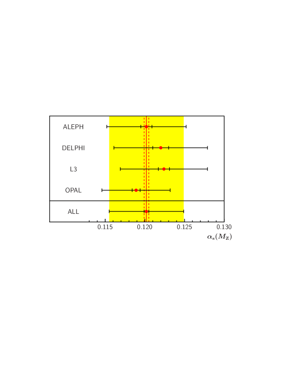
Each experiment has performed $\alpha_{\mathrm{s}}$ fits using these predictions for the six event shape variables at different $\sqrt{s}$. A preliminary combination of these results, taking into account the correlations between the sources of uncertainties, yields [6]

$$\alpha_{\rm s}(M_{\rm Z})=$$

$$0.1202\pm 0.0003(\mbox{stat})\pm 0.0007(\mbox{expt})$$

$$\pm 0.0015(\mbox{hadr})\pm 0.0044(\mbox{theo})$$

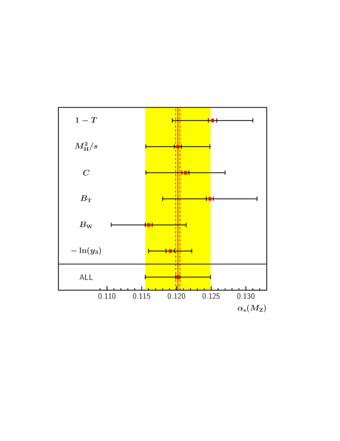
with $\chi^{2}/\mbox{d.o.f.}=93/166$. The combined $\alpha_{\mathrm{s}}$ measurements for each event shape variable are shown in Fig. 2 and the combined $\alpha_{\mathrm{s}}$ measurements for each experiment in Fig. 3.

Figure 3: Combined $\alpha_{\rm s}(M_{\rm Z})$ for the four LEP experiments using the measurements from the six event shape variables. The inner error bar is the statistical, the outer error bar is the total uncertainty [6].

Figure 4: The running of $\alpha_{\mathrm{s}}$ as a function of $Q=\sqrt{s}$ using the combined LEP data. The inner error bar is the statistical uncertainty, the outer error bar is the total uncertainty [6].

Table 1: Summary of the $\alpha_{\rm s}(M_{\rm Z})$ results presented in this talk.

	data	theory	$\alpha_{\rm s}(M_{\rm Z})$	stat	expt	hadr	theo
LEP	event shapes	$\mathcal{O}(\alpha_{\mathrm{s}}^{2})$+NLLA	0.1202	0.0003	0.0007	0.0015	0.0044
OPAL	radiative events	$\mathcal{O}(\alpha_{\mathrm{s}}^{2})$+NLLA	0.1176	0.0012	${}^{+0.0093}_{-0.0085}$
OPAL	$R_{4}$/Durham	$\mathcal{O}(\alpha_{\mathrm{s}}^{3})$+NLLA	0.1208	0.0006	0.0021	0.0019	0.0024
DELPHI	$R_{4}$/Cambridge	$\mathcal{O}(\alpha_{\mathrm{s}}^{3})$+$x_{\mu}^{\rm opt}$	0.1175	0.0005	0.0010	0.0027	0.0007

The experimental uncertainty includes uncertainties from cut variation, detector corrections and background subtraction. The hadronization uncertainty is determined by performing the hadronization correction using different MC generators (HERWIG, ARIADNE, PYTHIA. The theoretical uncertainty includes the variation of the renormalization scale, $0.5<x_{\mu}<2$, the variation of the logarithmic rescaling factor, $2/3<x_{L}<3/2$, and of kinematic cut-off parameters. In addition, the $\log(R)$ matching scheme is replaced by the $R$ matching scheme [7].

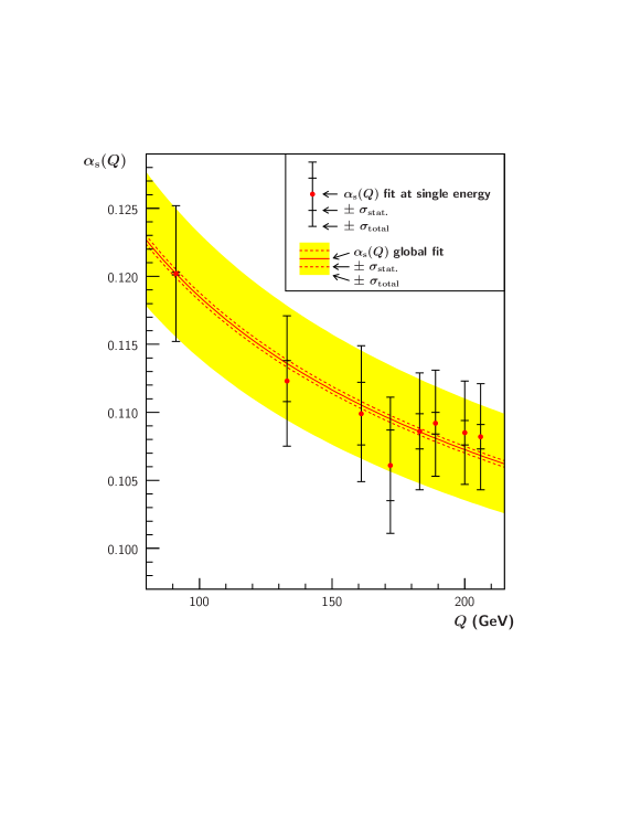
The running of $\alpha_{\mathrm{s}}$ using the combined data is shown in Fig.4. Although the statistical precision of the LEP1 data at $\sqrt{s}=M_{\rm Z})$ is much higher, the LEP1 and LEP2 data have about equal weight in the combined fit because of the smaller hadronization and theory uncertainties at larger $\sqrt{s}$.

3 $\bm\alpha_{\rm s}$ from Radiative Events

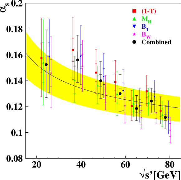
Radiative hadronic events have been used to extend the range of center-of-mass energies below $\sqrt{s}=M_{\rm Z}$. Assuming that initial state or final state photons do not interfere with the QCD process [8], a measurement of $\alpha_{\mathrm{s}}$ at a reduced center-of-mass energy $\sqrt{s^{\prime}}$ is possible by identifying isolated high energy photons in the detector [9].

Figure 5: The running of $\alpha_{\mathrm{s}}$ as a function of $Q=\sqrt{s^{\prime}}$ using radiative hadronic events measured by OPAL [10]. The result of the $\alpha_{\mathrm{s}}$ fit is shown as continuous line.

In the analysis performed by OPAL [10] photons have been separated from the dominant $\pi^{0}$ background by using a likelihood based on cluster shape fits in the calorimeter. The running of $\alpha_{\mathrm{s}}$ as function of $\sqrt{s^{\prime}}$ is shown in Fig. 5. The result of the $\alpha_{\mathrm{s}}$ fit is given in Table 1.

4 Power Law Corrections

Non-perturbative effects in event shape observables are usually suppressed by powers of $1/Q$ [11]. The corresponding hadronization corrections at LEP energies are of the order $10\%$. These hadronization corrections can be determined using MC generators or by analytical power law calculations. These calculations introduce one additional phenomenological parameter $\alpha_{0}$,

$$\alpha_{0}(\mu_{I})=\frac{1}{\mu_{I}}\int_{0}^{\mu_{I}}\alpha_{\mathrm{s}}(k)\mathrm{d}k,$$

which measures the effective strength of the strong coupling up to an infrared matching scale of $\mu_{I}\approx 1$ GeV. The parameter $\alpha_{0}$ is expected to be universal and must be determined by experiment.

Figure 6: Contours of confidence levels for simultaneous measurements of $\alpha_{\mathrm{s}}$ and $\alpha_{0}$ measured by L3 using the first moments of event shape variable. The unweighted averages are shown as shaded bands. A 4-jet observable (D parameter) is also shown.

Figure 7: Contours of confidence levels for simultaneous measurements of $\alpha_{\mathrm{s}}$ and $\alpha_{0}$ compared to the $\alpha_{\mathrm{s}}$ measurement using MC corrections (shaded band).

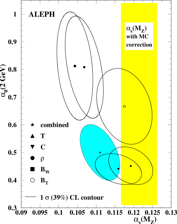
The result of such a combined fit, performed by L3 [4] for the first moments of the event shape variables, is shown in Fig. 6. The six values of $\alpha_{0}$ obtained from the event-shape variables do not agree well. A similar result has been obtained by DELPHI [3]. A large spread of $\alpha_{0}$ values has also been observed by ALEPH [2] using event shape distributions. The resulting $\alpha_{\mathrm{s}}$ is significantly lower than the result obtained using MC hadronization corrections (Fig. 7).

5 $\bm\alpha_{\mathrm{s}}$ from Four-jet Rates

An alternative method to determine $\alpha_{\mathrm{s}}$ is to measure four-jet rates, since the jet rates are predicted as functions of the jet resolution parameter with $\alpha_{\mathrm{s}}$ as free parameter. OPAL [12] has measured the four-jet rates using the Durham jet finding algorithm [1] as a function of the jet resolution parameter (Fig. 8). The strong coupling $\alpha_{\mathrm{s}}$ is fitted using a ${\cal O}(\alpha_{\mathrm{s}}^{3})$+NLLA matched calculation of the four-jet rates.

Figure 8: A fit to the four-jet rate $R_{4}$ measured at $\sqrt{s}=198$ GeV.

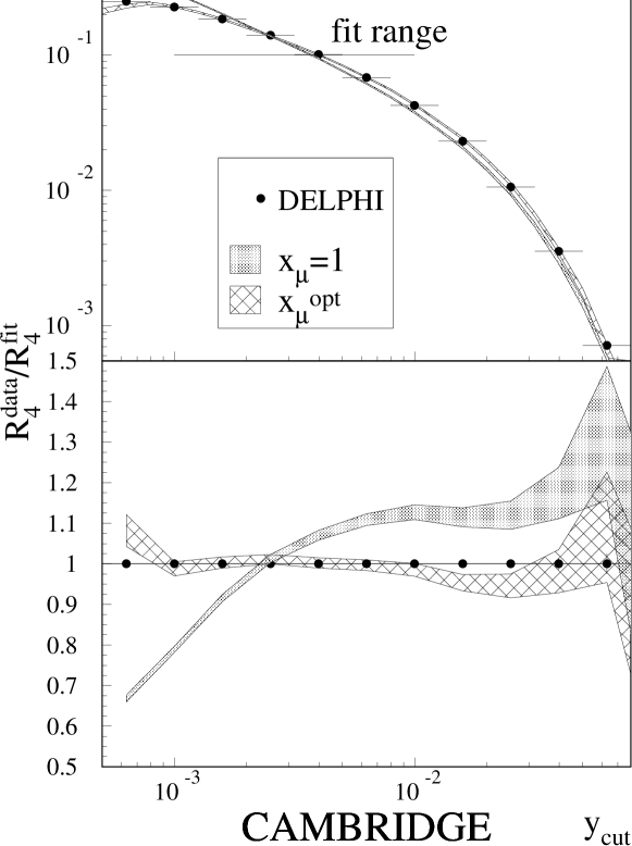
In a similar analysis, DELPHI [13] has measured the four-jet rates using the Durham and the Cambridge [14] algorithms. The data are fitted using a fixed order ${\cal O}(\alpha_{\mathrm{s}}^{3})$ calculation with both $\alpha_{\mathrm{s}}$ and the renormalization scale $x_{\mu}$ as free parameter. To determine the experimentally optimized scale, a two parameter fit with $\alpha_{\mathrm{s}}$ and $x_{\mu}^{\rm opt}$ as free parameters has also been performed (Fig. 9). Due to a smaller theoretical uncertainty the $\alpha_{\mathrm{s}}$ fit using the Cambridge algorithm is quoted as final result (Table 1).

Figure 9: Fits to the four-jet rates $R_{4}$ measured at $\sqrt{s}=M_{\rm Z}$ using the Cambridge algorithm. The grey band shows a fit with the physical scale ($x_{\mu}=1$) and the cross-hatched band a fit with optimized scales.

6 Summary

A preliminary $\alpha_{\mathrm{s}}$ combination using the final event shape measurements of all four LEP experiments has been presented. The universality of power law corrections has been studied. Radiative events and four-jet events have been used to study the running of $\alpha_{\mathrm{s}}$.

References

- [1] S. Catani et al., Phys. Lett. B 269, 432 (1991).
- [2] ALEPH Coll., A. Heister et al., Eur. Phys. J. C 35, 457 (2004).
- [3] DELPHI Coll., J. Abdallah et al., Eur. Phys. J. C 37, 1 (2004).
- [4] L3 Coll., P. Achard et al., Phys. Rept. 399, 71 (2004).
- [5] OPAL Coll., G. Abbiendi et al., CERN-PH-EP/2004-044, subm. to EPJC.
- [6] M. Ford and the LEP QCD Working Group, private communications.
- [7] R.W.L. Jones et al., JHEP 12, 7 (2003).
- [8] M. Dasgupta, G.P. Salam, J. Phys. G 30 R143 (2004), footnote 6.
- [9] L3 Coll., M. Acciarri et al., Phys. Lett. B 411, 339 (1997)
- [10] OPAL Coll., PN519 and abstract 5-0515.
- [11] Y. Dokshitzer, B.R. Webber, Phys. Lett. B 404, 321 (1997) and ref. therein.
- [12] OPAL Coll., PN527 and abstract 5-0600.
- [13] DELPHI Coll., J. Abdallah et al., hep-ex/0410071, subm. to EPJC.
- [14] Y. Dokshitzer et al., JHEP 8, 1 (1997).