Detection of $\pi^{+}\pi^{-}$atoms
with the DIRAC spectrometer at CERN

Abstract

The goal of the DIRAC experiment at CERN is to measure with high precision the lifetime of the $\pi^{+}\pi^{-}$ atom ($A_{2\pi}$), which is of order $3\times 10^{-15}$ s, and thus to determine the s-wave $\pi\pi$-scattering lengths difference $|a_{0}-a_{2}|$. $A_{2\pi}$ atoms are detected through the characteristic features of $\pi^{+}\pi^{-}$ pairs from the atom break-up (ionization) in the target. We report on a first high statistics atomic data sample obtained from p Ni interactions at 24 GeV/$c$ proton momentum and present the methods to separate the signal from the background.

Dedicated to the memory of Lucien Montanet

1 Introduction

The measurement of the lifetime of the $\pi^{+}\pi^{-}$ atom $A_{2\pi}$ [1], which is essentially determined by the $\pi^{+}\pi^{-}\rightarrow\pi^{0}\pi^{0}$ reaction, enables the determination of the combination $|a_{0}-a_{2}|$ of the s-wave $\pi\pi$-scattering lengths for isopins $I=0$ and $2$ in a model independent way [2, 3, 4, 5, 6, 7, 8] according to [7]

$$\frac{1}{\tau_{1s}}=\frac{2}{9}\;\alpha^{3}\;p\left|a_{0}-a_{2}\right|^{2}(1+\delta),$$ (1)

with $\tau_{1s}$ the lifetime of the atomic ground state, $\alpha$ the electromagnetic coupling constant, $p$ the $\pi^{0}$ momentum in the atomic c.m.s., and $\delta=(5.8\pm 1.2)\times 10^{-2}$ a correction due to QED and QCD [7].

The $\pi\pi$ scattering lengths $a_{0}$ and $a_{2}$ have been calculated within the framework of Chiral Perturbation Theory [9] by means of an effective Lagrangian with a precision at the percent level [10]. The lifetime of $A_{2\pi}$ in the ground state is predicted to be $\tau_{1s}=(2.9\pm 0.1)\times 10^{-15}$ s. These results are based on the assumption that the spontaneous chiral symmetry breaking is due to a strong quark condensate as recently suggested [11, 12]. An alternative scenario with an arbitrary value of the quark condensate [13] allows for larger $a_{0}$, $a_{2}$ compared with those of the standard scheme [10]. A measurement of the scattering lengths will thus contribute crucially to the current understanding of chiral symmetry breaking in QCD and constrain the magnitude of the quark condensate.

The differential production cross section of $A_{2\pi}$ atoms can be obtained from the double differential two-pion production cross section ($\sigma_{0}$) without a Coulomb final state interaction [14]:

$$\frac{d\sigma^{A}_{n}}{d{\vec{p}}_{A}}=(2\pi)^{3}\frac{E_{A}}{M_{A}}\;|\Psi_{n}(0)|^{2}\left.\frac{d\sigma_{0}}{d\vec{p}_{1}d\vec{p}_{2}}\right|_{\vec{p}_{1}=\vec{p}_{2}}\;,$$ (2)

where the differential production cross section $\sigma^{A}_{n}$ for atoms with principal quantum number $n$ and zero angular momentum depends on mass ($M_{A}$), momentum ($\vec{p}_{A}$) and energy ($E_{A}$) of the atom in the lab frame, and on the square of the Coulomb atomic wave function at zero distance $|\Psi_{n}(0)|^{2}$. The laboratory momenta of the $\pi^{+}$ and $\pi^{-}$ are denoted by $\vec{p}_{1},~{}\vec{p}_{2}$, respectively. On the basis of Eq. 2 and using the Fritiof 6 generator, yields for $A_{2\pi}$ in proton nucleus interactions have been calculated as a function of their energy and angle in the proton energy range from 24 GeV to 1000 GeV [14, 15, 16]. For a Ni target and a 24 GeV/c proton beam, $\sim 7\times 10^{-7}$ atoms are produced per proton interaction, of which, however, only $\sim 1\times 10^{-9}$ are detectable in the experiment, due to momentum and angular acceptance of the DIRAC apparatus.

The method for observing $A_{2\pi}$ and measuring its lifetime has been proposed in [14]. Pairs of $\pi^{+}\pi^{-}$ are produced mainly as unbound (”free”) pairs, but sometimes also as $A_{2\pi}$. The latter may either decay, get excited or break up into $\pi^{+}\pi^{-}$ pairs (atomic pairs) after interacting with target atoms. Due to their specific kinematical features, these atomic pairs are experimentally observable. For thin targets ($10^{-3}X_{0}$) the observable relative momentum $Q$ in the atomic pair system is $Q\leq 3$ MeV/$c$. Their yield is $\sim 10\%\div 20\%$ of the number of free pairs in the same $Q$ interval. In Fig. 2 the relative momentum distributions of atomic pairs are shown for $Q$ and $Q_{L}$ (relative momentum component along the flight direction of the pair) at the moment of break-up and at the exit of the target, as obtained with an event generator based on [17]. The number of atomic pairs is a function of the atom momentum and depends on the dynamics of the $A_{2\pi}$ interaction with the target atoms and on the $A_{2\pi}$ lifetime [18]. The theory of the $A_{2\pi}$ interaction with ordinary atoms allows the calculate of the relevant cross sections [17, 18, 19, 20, 21, 22, 23, 24, 25, 26, 27, 28]. For a given target thickness, the theoretical breakup probability for $A_{2\pi}$ is precise at the 1% level and uniquely linked to the lifetime of the atom [17, 29]. In Fig. 2 the break-up probability as a function of the lifetime is displayed for a 94 $\mu$m thick Ni target and for atomic pairs accepted in the DIRAC spectrometer.

Figure 1: Relative momentum distributions ($Q$, $Q_{L}$) for atomic $\pi^{+}\pi^{-}$ pairs at break-up and at the exit of the target (event generator, no spectrometer simulation). Note that $Q_{L}$ is almost not affected by multiple scattering in the target.

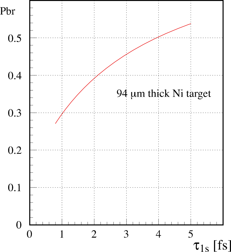
Figure 2: Break-up probability $Pbr$ as a function of the ground state lifetime $\tau_{1s}$ of the $A_{2\pi}$ atom for a Ni-target and DIRAC conditions.

The first observation of $A_{2\pi}$ [30] has been achieved in the interaction of 70 GeV/$c$ protons with Tantalum at the Serpukhov U-70 synchrotron. In that experiment, the atoms were produced in an $8\,\mu$m thick Ta target, inserted into the internal proton beam. With only $270\pm 50$ observed atomic pairs, it was already possible to set a lower limit on the $A_{2\pi}$ lifetime [31, 32]: $\tau>1.8\times 10^{-15}$ s $(90\%~{}CL)$.

In this paper, we present the first high statistics experimental data on $A_{2\pi}$ production on a Ni target at an external proton beam of the CERN PS and demonstrate the feasibility of the lifetime measurement. We are not attempting to deduce a lifetime here, as this requires a highly involved analysis of the normalization when evaluating the break-up probability.

2 The DIRAC experimental setup

The DIRAC setup is designed to detect oppositely charged pion pairs of low relative c.m. momenta with high resolution using a magnetic double arm spectrometer at a 24 GeV/$c$ extracted proton beam of the CERN PS and an especially low material budget in the secondary particle path. The spectrometer setup is shown in Fig. 3. A detailed description may be found in [33].

Figure 3: Schematic top view of the DIRAC spectrometer. Upstream of the magnet: target, microstrip gas chambers (MSGC), scintillating fiber detectors (SFD), ionization hodoscopes (IH) and iron shielding. Downstream of the magnet: drift chambers (DC), vertical and horizontal scintillation hodoscopes (VH, HH), gas Cherenkov counter (Ch), pre-shower detectors (PSh) and, behind the iron absorber, muon detectors (Mu).

The proton beam intensity during data taking was $0.9\times 10^{11}$ per spill with a spill duration of $400\div 450$ ms. The beam line was designed such as to keep the beam halo negligible [34]. The horizontal and vertical widths of the beam spot were $\sigma_{\mathrm{hor}}=(0.80\pm 0.08)$ mm and $\sigma_{\mathrm{vert}}=(1.60\pm 0.07)$ mm, respectively [35]. The targets we report here were 94 and 98 $\mu$m thick Ni foils, corresponding to $\sim 6.4\times 10^{-4}$ nuclear interaction probability [36] or $6.7\times 10^{-3}$ radiation length. The transverse dimensions of the circular targets (4.4 cm diameter) were sufficient to contain the proton beam fully and to exclude possible interactions of beam halo with the target holder.

The spectrometer axis is inclined upward by $5.7^{\circ}$ with respect to the proton beam. Particles produced in the target propagate in vacuum up to the upstream (with respect to the magnet) detectors and then enter into a vacuum chamber which ends at the exit of the magnet. The exit window is made of a 0.68 mm thick Al foil. The angular aperture is defined by a square collimator and is 1.2 msr ($\pm 1^{\circ}$ in both directions). The dipole magnet properties are $B=1.65$ T and $BL=2.2$ Tm.

The upstream detectors are 2.5 to 3 m away from the target and cover an area of roughly $10\times 10$ cm². The microstrip gas chambers (MSGC) consist of four planes: X, Y, U and V, with rotation angles of $0^{\circ}$, $90^{\circ}$, $5^{\circ}$, $85^{\circ}$ with respect to the X-plane. Each plane has 512 anode strips with a pitch of 0.2 mm. Clustering results in a spatial resolution for single tracks of 54 $\mu$m. The two planes (X, Y) of the scintillating fiber detector (SFD) provide both coordinate and timing information. Each plane contains 240 fiber columns (0.44 mm pitch), each column consisting of 5 fibers of 0.5 mm diameter. They are read out through multichannel position-sensitive photomultipliers and an analog signal processor that produces information for the appropriate TDC channel. The space and time resolutions are 130 $\mu$m (rms) and 0.8 ns, respectively. The analog signal processor merges two adjacent hits into one, depending on the relative pulse hight of the two signals and on their time difference. No merging takes place if the time difference is larger than 5 ns. The ionization hodoscopes (IH) serve for fast triggering and identification of unresolved double tracks through an energy loss measurement. The IH detector is composed of two vertical (X) and two horizontal (Y) layers, each with 16 slabs of plastic scintillator ($1\times 7\times 110$ mm³). The read-out provides logic (TDCs, trigger processors) and analog (ADCs) information. The total thickness of all upstream detectors, including the vacuum channel windows, is $6.0\times 10^{-2}X_{0}$.

The two arms of the spectrometer are identically equipped. Four sets of drift chambers are used (DC1 to DC4). DC1 and DC4 have two X and two Y planes each, DC1 has in addition two inclined W planes (11.3^∘ with respect to the X-wires). DC2 and DC3 have one X and one Y plane each. The sensitive areas range from $0.8\times 0.4$ m² to $1.28\times 0.4$ m², the signal wire pitch is 10 mm. The space resolution is better than 90 $\mu$m. The vertical hodoscopes (VH) supply time-of-flight information and serve trigger purposes. The hodoscope is made of 18 plastic scintillation counters ($2.2\times 7\times 40$ cm³). The time resolution is 127 ps. The horizontal hodoscope (HH) consists of 16 plastic scintillators ($2.5\times 2.5\times 130$ cm³). It serves essentially trigger purposes. The threshold Cherenkov detectors (Ch), are used to identify electrons (positrons) and to reject pairs containing an electron and/or a positron. The radiator is Nitrogen gas at normal pressure and ambient temperature. The average number of photoelectrons for particles with $\beta\approx$1 is larger than 16 and the efficiency more than 99.8%. Pion contamination above the detection threshold is estimated to be less than 1.5%. The pre-shower detector (Psh) consists of 8 elements, each comprising a Pb converter and a scintillator. Off-line analysis of the amplitudes from Psh provides additional $e$/$\pi$ separation. Each muon detector is made of a thick iron absorber followed by two planes of plastic-scintillator counters with 28 counters per plane.

The momentum range covered by the spectrometer is $1.2\div 8$ GeV/$c$. The relative resolution on the lab-momentum is dominated by the multiple scattering downstream of the vertical SFD detector and the spatial resolution of the drift chambers. While the former leads to a momentum independent resolution, the second leads to a slight increase with momentum. Studies of the $\Lambda$ signal in $\pi^{-}$p track pairs [37] result in $\sigma_{p}/p=2.8\times 10^{-3}$ and increasing to $3.3\times 10^{-3}$ at 8 GeV/$c$. The resolutions on the relative c.m.-momentum of $\pi^{+}\pi^{-}$ pairs from atomic break-up, $\vec{Q}=(Q_{x},Q_{y},Q_{L})$, are in the plane transverse to the total momentum $\vec{p}_{\pi^{+}\pi^{-}}^{~{}Lab}$, $\sigma_{Q_{x}}\approx\sigma_{Q_{y}}\leq 0.49$ MeV/$c$ and longitudinally $\sigma_{Q_{L}}=0.50$ MeV/$c$ [38] . The setup allows to identify electrons (positrons), protons with $p\leq 4$ GeV/$c$ (by time-of-flight) and muons (cf. Fig. 23 in [33]). It cannot distinguish $\pi$- from $K$-mesons, but kaons constitute a negligible contamination [16, 39].

The trigger system [40] reduces the event rate down to a level acceptable for the data acquisition system. The on-line event selection keeps almost all events with $Q_{L}<22$ MeV/$c$, $Q_{T}=\sqrt{Q_{x}^{2}+Q_{y}^{2}}<10$ MeV/$c$ and rejects events with $Q\geq 15$ MeV/$c$ progressively [41]. In the first level trigger [42] a coincidence of VH, HH and PSh signals and anticoincidence with Ch signals in both arms is treated as a pion-pair event. A condition on the HH of the positive and negative arms, $|\mathrm{HH}_{+}-\mathrm{HH}_{-}|\leq 2$ slabs, rejects events with $Q_{y}>10$ MeV/$c$. Fast hardware processors [40, 43, 44, 45] are used to decrease the first level trigger rate by a factor 5.5. The trigger rate in standard conditions was around 700 per spill. The trigger accepts events in a time window $\pm$20 ns with respect to the positive arm and thus allows for collecting also accidental events. The trigger system provides parallel accumulation of events from several other processes needed for calibration such as $e^{+}e^{-}$ pairs, $\Lambda\rightarrow p\pi^{-}$ or $~{}\pi^{\pm}\pi^{+}\pi^{-}$ final states.

The data acquisition [46, 47] accepted up to 2000 events per spill, at spill intervals as short as one second.

Dead times were studied in a run with 30% higher intensity than normal and depend on average beam intensity as well as on micro duty cycle of the beam. An overall dead time of 33% was found for triggers and data acquisition, with an additional 10% due to front-end electronics [48]. At normal intensities, dead times are lower. Biases due to dead times could not be found. When selecting data offline for further analysis, run periods, have been eliminated where problems with detectors or spill structure or micro duty cycle were found.

The full setup, including detectors, detector responses, read-outs, triggers and the magnet has been implemented into the detector simulation DIRAC-GEANT [49] and into the DIRAC analysis package ARIANE [50] such that simulated data can be treated in the same way as real measurements.

3 Track reconstruction

Events of interest consist of two particles of opposite charge with very low Q, resulting in two close lying tracks upstream that are separated downstream into the two arms of the spectrometer.

The magnetic field was carefully mapped and fine-tuned to a relative precision of $10^{-4}$. The final field map is used in the Monte Carlo GEANT simulation of the experiment [49]. For tracking, the field is summarized by a transfer function that uses as input the position, direction and momentum of a track in a reference plane at the exit of the magnet and calculates the position and direction of that track in a reference plane five meters upstream of the magnet. The transfer function consists of 4 polynomials with 5 parameters each.

Track reconstruction starts from the downstream part. A track candidate is searched for in the horizontal and vertical planes of the drift chambers separately. A ”horizontal” candidate must have a hit wire in one of the horizontal planes of the first (DC1) and last (DC4) chamber, as well as corresponding hits in the HH-detectors. They define a straight line. Hits close to that line are looked for in the other four horizontal planes of DC1 to DC4. Based on an acceptance window, a candidate is accepted if at least two more hits are found. The ”vertical” candidates are found analogously. Finally, candidates from horizontal and vertical wires are matched using the inclined planes. Projecting the spatial track parameters by means of the magnetic field polynomials to the center of the beam spot at the target provides a rough momentum estimate for each track candidate. Using this estimate and the precise position measurements deduced from drift-times, an overall track-fit for each candidate is made using a standard least-squares method, where the full error matrix is used, including the correlations (off-diagonal terms) induced by multiple scattering. Candidates are retained on the basis of a confidence level cut. The downstream track candidates are thus defined spatially with high precision. This is demonstrated in Fig. 5, where the difference between the measured hit coordinate in the first DC1 X-plane and the coordinate obtained with the track parameters at the same DC1 plane is shown. The spatial and angular resolutions depend on the particle momentum. They show a $1/p$ dependence and level off at 6 GeV/$c$. As an example the angular resolution in X direction is shown in Fig. 5. The one in the Y direction is about 4% better.

Figure 4: Difference between a hit coordinate measured by the first X-plane of DC in the right arm and a coordinate calculated with track parameters.

Figure 5: Resolution for angles of DC-tracks in X projections

The multiple scattering in the upstream detectors is such that in practice they have to be considered as the effective source of each track, and not the target as supposed above. Therefore, each of the above tracks, projected through the magnet onto the beam spot defines a reference line. Along this line, hit candidates are searched for in the upstream detectors within spatial windows defined mainly by multiple scattering and within time windows defined by the time-of-flight from the upstream detectors to the vertical hodoscopes downstream and their time resolutions.

Using all identified upstream information, a track-fit is made for each track-candidate by means of the Kalman-filter method [51], starting from the first downstream hit and ending at the exit window of the vacuum tube upstream of the MSGC detector.

With the hypothesis that the track originates from the target, the intersection of the proton beam with the target provides another measurement point for the Kalman filter, whose uncertainty is given by the measured intensity distribution of the proton beam across the target (cf. section 2) . A cut on the distance (15 mm) of the track from the beam spot leads to the final track selection [52].

Alternatively, assuming that a track pair originates from the same interaction, each pair candidate is fitted with the constraint that both tracks intersect in the central plane of the target (”vertex fit”). The complete $5\times 5$ uncertainty matrices of the two tracks are used. Tracks originating far from each other are rejected by a threshold confidence level. This procedure provides track parameters which are independent of the precise knowledge of the beam position and beam width. For the subsequent analysis these two procedures do not use the MSGCs, for reasons of optimum efficiency.

Full tracking uses MSGC and SFD to connect all upstream hits by straight lines. These track candidates are then matched with the downstream candidates. A vertex confidence level is calculated for each track pair, corresponding to the hypothesis that both tracks intersect at a common point lying on the target plane. Correlations from the estimated errors from multiple scattering are fully taken into account [53]. Both tracks are refitted at the end, under the constraint of having a common vertex [54].

To illustrate that the reconstructed events do in fact originate from the target, the distances between two tracks at the target are shown in Fig. 7. No vertex fit was done for these data.

Figure 6: Distances $\Delta x$ and $\Delta y$ between two reconstructed tracks at the target in the transverse plane.

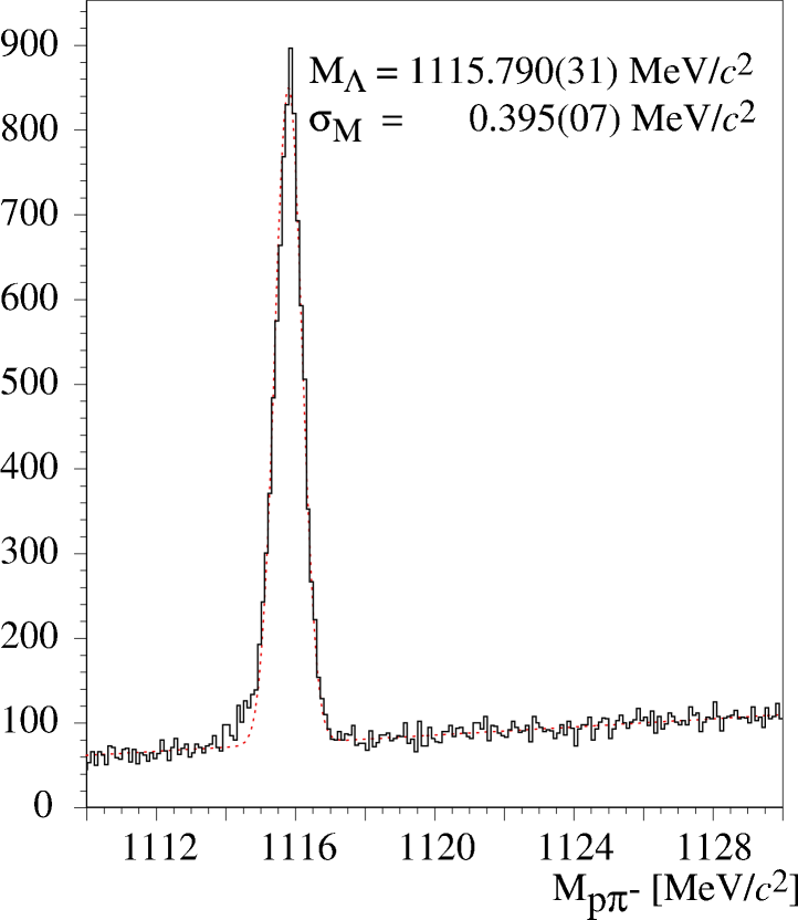
Figure 7: Invariant proton-pion mass ($M_{p\pi^{-}}$) distribution. The dashed line represents a fit of a Gaussian plus a straight line.

The correctness of the alignment and magnetic field description were verified by studying the decay of $\Lambda$ particles [55]. Events with one downstream track per spectrometer arm and a time-of-flight difference between the positive particle and the negative one between 0 and 1.3 ns were selected. Fig. 7 shows, for a typical control data sample, the invariant mass distribution from the two tracks under the hypothesis proton-pion. A fit of a Gaussian on a linear background yields $M_{\Lambda}=(1115.790\pm 0.031_{stat})$ MeV/$c^{2}$ with $\sigma_{M_{\Lambda}}=(0.395\pm 0.007_{stat})$ MeV/$c^{2}$. The measured width is entirely due to track reconstruction. The difference ($M_{p\pi^{-}}-M_{\Lambda}(PDG$ [36])) in units of the reconstruction error provides a measure of the correctness of the error estimation. The resulting distribution is fitted by a Gaussian with $\sigma=1.028\pm 0.006$, showing that the reconstruction errors are slightly underestimated. The same distribution was studied as a function of the pion momentum and found to be independent of it. The long term stability of the apparatus has been controlled using the $\Lambda$ mass and the corresponding widths.

4 Selection criteria

An event is rejected if more than two downstream tracks in either of the two arms are reconstructed. For each track the associated VH and HH hodoscope slabs are required. In the case of two tracks in one arm, the earlier in time is taken for further analysis. Events with more than one track per arm constitute less than 4% of the event sample.

Horizontal and vertical SFD hit candidates to be associated with a track (see section 3 for first momentum estimation) must have times within a window of $\pm 4$ ns (corresponding to $\pm 5\sigma$) with respect to the associated VH slab. Moreover, the hit candidates must be found in a spatial window of $\pm(0.2+4.8/p~{}[\mathrm{GeV/}c])$ cm (corresponding to $\pm 6\sigma$) with respect to the point of intersection of the track candidate with the SFD plane. This window is defined by multiple scattering in the downstream material when backward-extrapolating the track. At least one hit candidate is required. If there are more than four, the four closest to the window center are kept.

After the first stage of Kalman filtering, only events are kept with at least one track candidate per arm with a confidence level better than 1% and a distance to the beam spot in the target smaller than 1.5 cm in x and y. For such tracks, the SFD hits are redetermined in a narrower ($\pm 1$cm) window around the new track intersect. Events with less than four hits in the window per SFD plane and not more than six in both planes are retained. Finally, all track pairs with $|Q_{x}|<6$ MeV/$c$, $|Q_{y}|<6$ MeV/$c$ and $|Q_{L}|<45$ MeV/$c$ are selected for further analysis.

This preselection procedure retains 6.2% of the $\pi\pi$ data obtained with the Ni target in 2001. The time difference between the positive and the negative arm, measured by the VHs, for events that passed the preselection criteria is shown in Fig. 9.

For the final analysis further cuts and conditions are applied:

• ”prompt” events are defined by a time difference (corrected for the flight path assuming pions) measured by the VHs between the positive and the negative arm, $|\Delta t|\leq 0.5$ ns, corresponding to a $\pm 2.7\sigma$ cut.

• ”accidental” events are defined by time intervals $-15$ ns$\leq\Delta t\leq-5$ ns and 7 ns$\leq\Delta t\leq 17$ ns, conditioned by the read-out features of the SFD detector (cf. section 2) and suppressing protons (cf. Fig. 9).

• protons in prompt events are rejected by requiring momenta of the positive particle to be $p_{+}\leq 4$ GeV/$c$.

• $e^{\pm}$ and $\mu^{\pm}$ are rejected through appropriate cuts on the Cherenkovs, the Pre-shower and the Muon counters [56].

• $Q_{T}\leq 4$ MeV/$c$ and $|Q_{L}|<22$ MeV/$c$. The $Q_{T}$ cut preserves 98% of the atomic signal, the $Q_{L}$ cut preserves background outside the signal region for defining the background below the signal.

• the vertex-fit with highest confidence level from track and vertex fits is retained.

• only events with at most two preselected hits per SFD plane are accepted. This provides the cleanest possible event pattern. This criterion is not used with the full tracking (cf. section 3).

Figure 8: Time difference between positive and negative vertical hodoscope slabs associated with the selected tracks. The asymmetry for positive differences is due to time correlated protons.

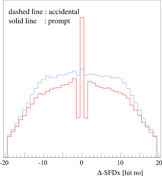
Figure 9: Difference in hit number for selected SFD hits in the X-plane, for accidental and prompt events. Note the effect of merging of adjacent hits for prompt events. Arbitrary scale.

5 Signal and background in $\pi^{+}\pi^{-}$ atom detection

Once produced in proton-nucleus interactions, all $A_{2\pi}$ atoms will annihilate if they propagate in vacuum. In a finite target, however, they interact electromagnetically with the target atoms, and some of them break up. The event generator for $\pi^{+}\pi^{-}$ pairs from $A_{2\pi}$ break-up yielded $Q$ and $Q_{L}$ distributions shown in Fig. 2 (cf. section 1). At the exit of the target, multiple scattering has caused a considerable broadening of the $Q$-distribution while the $Q_{L}$ distribution has remained unchanged. The $Q_{L}$ distribution at break-up is already much narrower than the $Q$-distribution because the break-up mechanism itself affects mostly $Q_{T}$ (analogous to $\delta$ electron production). These features led us to consider in the analysis not only $Q$ but also $Q_{L}$ distributions .

The atomic pairs are accompanied by a large background. The $Q$ distribution of all $\pi^{+}\pi^{-}$ pairs produced in single proton-nucleus interactions in the target is described by:

$$dN/dQ=dN_{\rm C}/dQ+dN_{\rm nC}/dQ+dn_{A}/dQ.$$ (3)

$N_{\rm C}$ is the number of $\pi^{+}\pi^{-}$ pairs originating from short-lived sources (fragmentation, rescattering, mesons and excited baryons that decay strongly). These pairs undergo Coulomb interaction in the final state (Coulomb pairs). $N_{\rm nC}$ is the number of $\pi^{+}\pi^{-}$ pairs with at least one particle originating from long-lived sources (mesons and baryons that decay electromagnetically or weakly). They do not exhibit Coulomb final state interaction (non-Coulomb pairs). Finally, $n_{A}$ is the number of $\pi^{+}\pi^{-}$ pairs from $A_{2\pi}$ break-up.

Accidental $\pi^{+}\pi^{-}$ pairs ($dN_{\rm acc}/dQ$) originate from different proton-nucleus interactions and are uncorrelated in time, i.e. they are neither affected by Coulomb nor by strong interaction in the final state. Such events may also belong to the time window that defines prompt events (see section 4).

These backgrounds, as they are measured and reconstructed, are needed for subtraction from the measured data in order to obtain the excess produced by the atomic signal. The backgrounds may be obtained in different ways.

One method is based on a Monte Carlo modelling of the background shapes using special generators for the non-Coulomb (nC) and Coulomb (C) backgrounds and accidental pairs [57]. Uniformity in phase space is assumed for the backgrounds ($dN/dQ\sim Q^{2}$), modified by the theoretical Coulomb correlation function $A_{\rm C}^{\rm theo}(Q)$ [58] for C-background. Effects of the strong final state interaction and the finite size of the pion production region [59] on the Coulomb correlation function are small and neglected here. The differences of pion momentum distributions for the different origins of $\pi^{+}\pi^{-}$ pairs are implemented (cf. [60, 57]). The generated events are propagated through the detector (GEANT [49]). Simulating the detectors, detector read-outs and triggers and analyzing the events using the ARIANE analysis package of DIRAC [50] result in the high statistics distributions $dN_{\rm C}/dQ$, $dN_{\rm nC}/dQ$ (cf. Eq. 3) , and $dN_{\rm acc}/dQ$. These distributions are used later to analyze the measured distributions. Though not necessary for the signal extraction, the $A_{2\pi}$ signal was also simulated yielding $dn_{A}/dQ$. Monte Carlo simulated distributions were generated with about 10 times the statistics of the measured data. The simulated backgrounds were obtained with dedicated generators, without any additional tracks from the proton nucleus interaction. A special Monte Carlo simulation with additional background tracks leads essentially to a reduction in reconstruction efficiency.

The second method circumvents the Monte Carlo simulations of background, detectors and triggers by relating the backgrounds to the measured accidental background. It was successfully applied in [30]. The assumption is that accidentals can be used to describe the distribution of free $\pi^{+}\pi^{-}$ pairs, which then must be corrected for final state interactions. By denoting $\Phi(Q)\equiv dN_{\rm acc}^{meas}/dQ$, the experimental correlation function $R(Q)$ is given by:

$$R(Q)=\frac{1}{\Phi(Q)}\left(\frac{dN_{\rm nC}}{dQ}+\frac{dN_{\rm C}}{dQ}\right)=N\times[f+A_{\rm C}(Q)]$$ (4)

Here $A_{C}(Q)$ is the Coulomb enhancement function [58] smeared by multiple scattering in the target and the finite setup resolution. In practice it can not be obtained by folding procedures but must be obtained from Monte Carlo simulations described above. $N$ and $f$ are free parameters, and $\Phi(Q)$ is the measured spectrum of accidentals corrected for the differences between prompt and accidental momentum distributions [60].

The measured accidental distributions had to be corrected for the different recording conditions as compared to prompt events, such as the SFD merging of adjacent hits, or track identification by time, which is impossible for prompt events in case of ambiguities. In Fig. 9 the difference in selected SFD hits is shown for accidental and prompt events for the X-plane (the Y-plane is similar). The merging feature of the SFD read-out together with a $\sim$ 5% single track inefficiency of the SFD lead to the enhancement for $\Delta$-SFD=0, and to the dips left and right of it.The correction of the measured accidental spectra for prompt conditions was done in two ways. On an event by event basis adjacent hits of the measured accidentals were merged into one hit according to the measured probability, and that hit was given the times of the two original hits. Then tracking was started, and the timing conditions could be applied as described above (cf. section 4). An other way of correcting was to construct accidental distributions from uncorrected events, but giving up the timing conditions. The resulting distributions were then given weights according to the measured merging probabilities.

6 Experimental data and atomic signal extraction

DIRAC began data taking in autumn 1999. Here we present data taken in 2001 using 94 $\mu$m and 98 $\mu$m thick Nickel targets. The integrated proton flux through the target for these data is $8.6\times 10^{16}$, corresponding to $5.5\times 10^{13}$ pNi interactions and to $6.4\times 10^{8}$ recorded $\pi\pi$ triggers. The reconstructed accidental and prompt $\pi\pi$ pairs (see Section 4 for the cuts) are shown in Fig. 10.

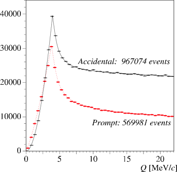
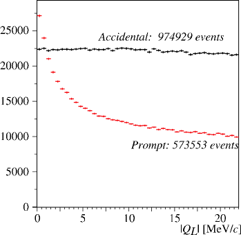
Figure 10: Experimental $Q$ and $Q_{L}$ distributions for prompt and accidental $\pi\pi$ events. Continuous lines serve as guides for the eye. The sharp peak at $Q=4$ MeV/$c$ is due to the cut $Q_{T}\leq 4$ MeV/$c$. The number of events is given for the displayed momentum window, the bin-width is 0.5 MeV/$c$. Note the strong Coulomb enhancement in the $Q_{L}$ distribution for prompt events.

The Monte Carlo backgrounds or the correlation function $R(Q)$ (cf. Section 5) are fitted to the measured prompt spectra in $Q$ and $Q_{L}$ intervals which exclude the atomic signal (typically $Q>4$ MeV/$c$, $Q_{L}>2$ MeV/$c$). The amount of time-uncorrelated events in the prompt region was determined to be 6.5% of all prompt events by extrapolating the accidental $\Delta t$ distribution to zero and was subtracted from the prompt distributions (cf. Fig. 9). The fits provide the relative amounts of non-Coulomb and Coulomb backgrounds and the parameters $N$ and $f$ of Eq. 4. As a constraint, these background components must be the same for $Q$ and $Q_{L}$.

The analysis using Monte Carlo backgrounds and no vertex fit is summarized in Fig. 11. The background composition is indicated, and the excess at low $Q$ and $Q_{L}$ is clearly seen. Subtraction provides the residuals, also shown in Fig. 11, which represent the atomic signals. As expected from Fig. 2, the signal is narrower in $Q_{L}$ than in $Q$. The simulated shape is in agreement with the data. The signal strength has to be the same in $Q$ and $Q_{L}$ if the background is properly reconstructed. The observed difference demonstrates that the backgrounds are consistent at the per mille level. The fact that outside of the signal region the residuals are perfectly zero demonstrates the correctness of the Monte Carlo simulation.

Figure 11: Top: Experimental $Q$ and $Q_{L}$ distributions after subtraction of the time uncorrelated background, approximated with Monte Carlo backgrounds (dashed lines). Bottom: Residuals after background subtraction. The dashed lines represent the expected atomic signal shape. Notice that the signal strengths in $Q$ and $\mathrm{Q_{L}}$ are about the same. The bin-width is 0.25 MeV/$c$.

The results of the analysis using the accidentals as a basis for background modelling are shown in Fig. 12. The clear deviation of $R(Q)$ at low $Q$ from unity is due to the attractive Coulomb interaction in the final state. There is good agreement between the experimental and fitted ”correlation” function $R$ for $Q>2.5$ MeV/$c$, whereas for $Q<2.5$ MeV/$c$ the experimental correlation function (left hand side of Eq. 4) shows significantly higher values, due to the presence of atomic pairs. In order to extract the number of atomic pairs the fit function (right hand side of Eq. 4) has been multiplied by the accidental distribution $\Phi(Q)$. The subtraction of the latter from the full measured spectrum leads to the atomic pair signal in Fig. 12.

Figure 12: Top: Experimental $Q$ and $Q_{L}$ correlation functions (experimental points). The background correlation function is shown as a smooth curve. Bottom: Residuals after background subtraction. The dashed lines represent the expected atomic signal shape. The bin-width is 0.5 MeV/$c$.

Based on the same data sample of preselected events, the analysis using Monte Carlo backgrounds and no vertex fit was repeated allowing for three hits instead of only two in the search window (cf. section 4) and selecting the hit closest to the search reference trajectory. This yields about 25% more events in the signal, but 43% more in total (see Table 1), thus the signal/background quality diminishes.

An analysis fully independent on the upstream detectors was done using only information from the downstream detectors. Events were selected from raw data along with a looser cut in $Q_{T}$. The particles were assumed to be emitted from the center of the beam spot at the target. For this analysis only the $Q_{L}$ distribution shows a signal, because multiple scattering in the upstream detectors does not distort $Q_{L}$ so much but destroys $Q_{T}$ and hence $Q$. With respect to the standard selection the signal increases by about 40-50%. The total number of events is, however, almost 3.5 times larger (see Table 1). The background increases with respect to the standard selection by a factor of two because of the loose cut on $Q_{T}\leq 6$MeV/$c$. Moreover, signal and background increase because

• no cut on the multiplicity two in the SFD search window is needed (gain $\geq 25$%).

• no detector response of the SFD is needed (gain due to single track efficiency of 95% for two tracks in two planes $\geq 23$%.).

Table 1: Reconstructed atomic pair events for $Q$ and $Q_{L}$ using full tracking and Monte Carlo background (Full), no vertex fit and Monte Carlo background (MC), vertex fit and background reconstruction from accidentals (ACC), as ”MC” but using up to 3 hits instead of two in the SFD acceptance (MC-3 hits), and reconstruction only with downstream detectors (Down). Full selected data sample used for signal extraction (integral from 0 to 15 MeV/$c$) for each method (selected sample), and ratio of extracted signal and selected data sample ($\frac{\mathrm{signal}\;Q_{L}}{\mathrm{selected\;sample}}$).

• 	Full	MC	ACC	MC-3 hits	Down
  $Q$	$5526\pm 385$	$6520\pm 370$	$4670\pm 930$	8230$\pm$440	-
  $Q_{L}$	$5322\pm 350$	$6510\pm 330$	$5730\pm 580$	8050$\pm$380	$9280\pm 970$
  selected sample	$\sim 429000$	$437060$	$385870$	624880	1503700
  $\frac{\mathrm{signal~{}}Q_{L}}{\mathrm{selected~{}sample}}$	1.24%	1.49%	$1.48\%$	1.29%	0.6%

The results are summarized in Table 1. The column ”Full” shows the results obtained with full tracking (cf. section 3) and background from Monte Carlo. The column ”MC” shows the result from reconstruction using Monte Carlo backgrounds and no vertex fit [61]. The column ”ACC” shows the result of reconstruction using the measured accidentals and vertex fit. The column ”MC-3 hits” is analogous to column ”MC” but allowing for 3 hits in the SFD planes [61] instead of two (cf. section 4). The column ”Down” shows the result of using only the downstream detectors and the background reconstruction based on accidentals. The integral (0 to 15 MeV/$c$) number of events retained after the specific selection cuts of each analysis methods is also given. The integral number of measured accidentals (needed for background reconstruction for col. ”ACC”) is about the same as the number of prompt events. The last row of Table 1 shows the signal fraction extracted from the selected data sample.

In the case of full tracking (col. ”Full” in Table 1) the integrated luminosity was (for the Ni-runs in 2001) only 79% of the preselected data due to the availability of the MSGC detector. Moreover, these data were not subject to a cut on 2 hits in the SFD (section 4) and thus should be compared with column ”MC-3 hits” of Table 1.

First we observe that the number of events in the full sample depends on the details of the cut procedures and selection methods. Using downstream detectors only (col.”down” of Table 1) results in a background much larger than the signal increase.

The consistency of the signal is satisfactory as can be seen from Table 1. The signal fractions of the selected data sample are the same for the Monte Carlo based method and the method based on accidentals (Table 1, columns ”MC” and ”ACC”), and very similar for full tracking and MC-3 hits (Table 1, columns ”Full” and ”MC-3 hits”). The large errors of column ”ACC” of Table 1 are due to the limited statistics of the measured accidentals. The difference in signal strength for $Q$ and $Q_{L}$ is due to slightly different fit regions for $Q$ ($Q_{T}<4$ MeV/$c$, $|Q_{L}|<22$ MeV/$c$, $Q>4$ MeV/$c$) and $Q_{L}$ ($Q_{T}<4$ MeV/$c$, 2 MeV/$c<|Q_{L}|<22$ MeV/$c$) and for signal searching ($Q<4$ MeV/$c$ and $|Q_{L}|<2$ MeV/$c$, respectively). Thus, the backgrounds in $Q$ and $Q_{L}$ are not identical and fluctuations of the background differences in the prompt data and in the measured accidental data lead to the (accidentally large) difference in the signal. The same argument holds for the Monte Carlo based method. However, there the statistical fluctuations of the background are negligible as compared to the measured data. Allowing for three hits instead of two in the SFDs yields about the same number of events in the signal as were found without using any upstream detector. This indicates that the main source of loss in signal is inefficiency in the upstream detectors.

7 Conclusion

For the first time a large statistics sample of $\pi^{+}\pi^{-}$ pairs from atom break-up has been detected. Independent tracking procedures and complementary background reconstruction strategies lead to compatible results. The background as obtained with Monte Carlo methods is in excellent agreement with the data. We conclude that severe systematic errors may be excluded when extracting the atomic pair signal. The statistical accuracy of the signal allows for an estimated statistical error on the lifetime of the $A_{2\pi}$ atom of about 15% [61]. In this paper we have analysed only part of our data. In view of the full statistics accumulated by the experiment so far and with systematic errors estimated to be smaller than the statistical ones [61] the goal of the experiment to achieve a 10% accuracy for the lifetime of the $A_{2\pi}$ atom is in reach.

References

References

- [1] Adeva B et al., DIRAC proposal, CERN/SPSLC 95-1, SPSLC/P 284 (1995)
- [2] Deser S et al., Phys. Rev. 96 (1954) 774
- [3] Uretsky J and Palfrey J, Phys. Rev. 121 (1961) 1798
- [4] Bilenky S M et al., Yad. Fiz. 10 (1969) 812; (Sov. J. Nucl. Phys. 10 (1969) 469)
- [5] Jallouli H and Sazdjian H, Phys. Rev. D58 (1998) 014011; Erratum: ibid. D58 (1998) 099901
- [6] Ivanov M A et al. Phys. Rev. D58 (1998) 094024
- [7] Gasser J et al., Phys. Rev. D64 (2001) 016008; hep-ph/0103157
- [8] Gashi A et al., Nucl. Phys. A699 (2002) 732
- [9] Weinberg S, Physica A96 (1979) 327; Gasser J and Leutwyler H, Phys. Lett. B125 (1983) 325 and Nucl. Phys. B250 (1985) 465, 517, 539
- [10] Colangelo G, Gasser J and Leutwyler H, Nucl. Phys. B603 (2001) 125
- [11] Colangelo G, Gasser J and Leutwyler H, Phys. Rev. Lett. 86 (2001) 5008
- [12] Pislak S et al., Phys. Rev. Lett. 87 (2001) 221801
- [13] Knecht M et al., Nucl. Phys. B457 (1995) 513
- [14] Nemenov L L, Yad. Fiz. 41 (1985) 980; (Sov. J. Nucl. Phys. 41 (1985) 629)
- [15] Gorchakov O E et al., Yad. Fiz. 59 (1996) 2015; (Phys. At. Nucl. 59 (1996) 1942)
- [16] Gorchakov O E et al., Yad. Fiz. 63 (2000) 1936; (Phys. At. Nucl. 63 (2000) 1847)
- [17] Schumann M et al., J. Phys. B 35 (2002) 2683.
- [18] Afanasyev L G and Tarasov A V, Yad. Fiz. 59 (1996) 2212, (Phys. At. Nucl. 59 (1996) 2130)
- [19] Dulian L S and Kotsinian A M, Yad. Fiz. 37 (1983) 137; (Sov. J. Nucl. Phys. 37 (1983) 78)
- [20] Mrówczyński S, Phys. Rev. A33 (1986) 1549; Mrówczyński S, Phys. Rev. D36 (1987) 1520; Denisenko K G and Mrówczyński S, ibid. D36 (1987) 1529
- [21] Halabuka Z et al., Nucl. Phys. B554 (1999) 86
- [22] Tarasov A V and Khristova I U, JINR-P2-91-10, Dubna 1991
- [23] Voskresenskaya O O, Gevorkyan S R and Tarasov A V, Phys. At. Nucl. 61 (1998) 1517
- [24] Afanasyev L, Tarasov A and Voskresenskaya O, J. Phys. G 25 (1999) B7
- [25] Ivanov D Yu, Szymanowski L, Eur. Phys. J. A5 (1999) 117
- [26] Heim T A et al., J Phys B 33 (2000) 3583
- [27] Heim T A et al., J Phys B 34 (2001) 3763
- [28] Afanasyev L, Tarasov A and Voskresenskaya O, Phys. Rev. D 65 (2002) 096001; hep-ph/0109208
- [29] Santamarina C et al., J Phys B 36 (2003) 4273
- [30] Afanasyev L G et al., Phys. Lett. B308 (1993) 200
- [31] Afanasyev L G et al., Phys. Lett. B338 (1994) 478
- [32] Afanasyev L G et al., Communication JINR P1-97-306, Dubna, 1997
- [33] Adeva B et al., Nucl. Instr. Meth. A515 (2003) 467
- [34] Ferrando O and Hemery J-Y, CERN-PS Division, PS/ CA/ Note97-16
- [35] Lanaro A, DIRAC note 2002-01, http://dirac.web.cern.ch/DIRAC/i_notes.html
- [36] Hagiwara K et al. (PDG), Phys. Rev. D66 (2002) 010001
-
[37]
Adeva B, Romero A and Vazquez Doce O,
DIRAC note 2004-05,
http://dirac.web.cern.ch/DIRAC/i_notes.html -
[38]
Gortchakov O and Santamarina C,
DIRAC note 2004-01,
http://dirac.web.cern.ch/DIRAC/i_notes.html - [39] Adeva B et al., Nucl. Instr. Meth. A491 (2002) 41
- [40] Afanasyev L et al. Nucl. Instr. Meth. A491 (2002) 376
- [41] Vlachos S, DIRAC note 2003-04, http://dirac.web.cern.ch/DIRAC/i_notes.html
- [42] Afanasyev L et al., Nucl. Instr. Meth. A479 (2002) 407
- [43] Gallas M, Nucl. Instr. Meth. A481 (2002) 222
- [44] Kokkas P et al., Nucl. Instr. Meth. A471 (2001) 358
- [45] Vlachos S, DIRAC note 2000-13, http://dirac.web.cern.ch/DIRAC/i_notes.html
- [46] Olshevsky V G, Trusov S V, Nucl. Instr. Meth. A469 (2001) 216
- [47] Karpukhin V et al., Nucl. Instr. Meth. A512 (2003) 578
- [48] Kulikov A, Zhabitsky M, Nucl. Instr. Meth. A527 (2004) 591
- [49] GEANT3 for DIRAC, version 2.63, unpublished, http://dirac.web.cern.ch/DIRAC/
- [50] Analysis software package for DIRAC, unpublished
- [51] Maybeck P, Stochastic Models, Estimation and Control, Vol. 1. Academic Press, New York (1979)
- [52] Ch. Schuetz P and Tauscher L, DIRAC note 02-01, Ch. Schuetz P and Tauscher L, DIRAC note 03-06, http://dirac.web.cern.ch/DIRAC/i_notes.html
- [53] Pentia M et al., Nucl. Instr. Meth. A369 (1996) 101; Pentia M and Constantinescu S, DIRAC note 01-04, http://dirac.web.cern.ch/DIRAC/i_notes.html
-
[54]
Adeva B, Romero A and Vazquez Doce O, DIRAC note
2003-08,
http://dirac.web.cern.ch/DIRAC/i_notes.html - [55] Kokkas P, DIRAC note 2004-04, http://dirac.web.cern.ch/DIRAC/i_notes.html
-
[56]
Brekhovskikh V and Gallas M V, DIRAC note
2001-02,
http://dirac.web.cern.ch/DIRAC/i_notes.html -
[57]
Santamarina C and Ch. Schuetz P, DIRAC note
2003-09,
http://dirac.web.cern.ch/DIRAC/i_notes.html - [58] Sakharov A D, Zh. Eksp. Teor. Fiz. 18 (1948) 631
- [59] Lednicky R, Lyuboshitz V L, Yad. Fiz. 35 (1982) 1316 (Sov. J. Nucl. Phys. 35 (1982) 770)
- [60] Lanaro A, DIRAC note 2001-01, http://dirac.web.cern.ch/DIRAC/i_notes.html
-
[61]
Ch. Schuetz P, Thesis, Basel University, March
2004,
http://cdsweb.cern.ch/search.py?recid=732756