Measurement of the $\chi_{c2}$ Polarization in $\psi(2S)\rightarrow\gamma\chi_{c2}$

Abstract

The polarization of the $\chi_{c2}$ produced in $\psi(2S)$ decays into $\gamma\chi_{c2}$ is measured using a sample of $14\times 10^{6}$ $\psi(2S)$ events collected by BESII at the BEPC. A fit to the $\chi_{c2}$ production and decay angular distributions in $\psi(2S)\rightarrow\gamma\chi_{c2}$, $\chi_{c2}\rightarrow\pi^{+}\pi^{-}$ and $K^{+}K^{-}$ yields values $x=A_{1}/A_{0}=2.08\pm 0.44$ and $y=A_{2}/A_{0}=3.03\pm 0.66$, with a correlation $\rho=0.92$ between them, where $A_{0,1,2}$ are the $\chi_{c2}$ helicity amplitudes. The measurement agrees with a pure $E1$ transition, and $M2$ and $E3$ contributions do not differ significantly from zero.

I Introduction

The radiative transition between charmonium states has been studied extensively by many authors PRD42p2293 ; PRD21p203 ; PRD26p2295 ; PRD25p2938 ; PRD28p1692 ; PRD28p1132 . In general, it is believed that $\psi(2S)\rightarrow\gamma\chi_{cJ}$ is dominated by the $E1$ transition, but with some $M2$ (for $\chi_{c1}$ and $\chi_{c2}$) and $E3$ (for $\chi_{c2}$) contributions due to the relativistic correction. These contributions have been used to explain the big differences between the calculated pure $E1$ transition rates and the experimental results PRD21p203 . They will also affect the angular distribution of the radiative photon. Thus the measurement of the angular distribution may be used to determine the contributions of the higher multipoles in the transition.

Furthermore, for $\psi(2S)\rightarrow\gamma\chi_{c2}$, the $E3$ amplitude is directly connected with $D$-state mixing in $\psi(2S)$ which has been regarded as a possible explanation of the large leptonic annihilation rate of $\psi(3770)$ PRD28p1132 . Since recent studies wympspp ; wymkskl also suggest the $S$- and $D$-wave mixing of $\psi(2S)$ and $\psi(3770)$ may be the key to solve the longstanding “$\rho\pi$ puzzle” and to explain $\psi(3770)$ non-$D\bar{D}$ decays, the experimental information on multipole amplitudes gains renewed interest.

Decay angular distributions were studied in $\psi(2S)\rightarrow\gamma\chi_{c2}$ by the Crystal Ball experiment using $\psi(2S)\rightarrow\gamma\gamma J/\psi$ Cball ; the contribution of the higher multipoles were not found to be significant but the errors were large due to the limited statistics. In the present analysis, $\psi(2S)\rightarrow\gamma\chi_{c2}\to\gamma\pi^{+}\pi^{-}$ or $\gamma K^{+}K^{-}$ decays will be used for a similar study. The analysis on these channels has the advantage that there is no background from $\chi_{c1}$ since the $\chi_{c1}\to\pi^{+}\pi^{-}$ and $K^{+}K^{-}$ processes are forbidden by parity conservation.

II The BES Experiment

The data used for this analysis are taken with the BESII detector at the BEPC storage ring operating at the $\psi(2S)$. The number of $\psi(2S)$ events is $14.0\pm 0.6$ million moxh , determined from the number of inclusive hadrons.

The Beijing Spectrometer (BES) detector is a conventional solenoidal magnet detector that is described in detail in Ref. bes ; BESII is the upgraded version of the BES detector bes2 . A 12-layer vertex chamber (VC) surrounding the beam pipe provides trigger information. A forty-layer main drift chamber (MDC), located radially outside the VC, provides trajectory and energy loss ($dE/dx$) information for charged tracks over $85\%$ of the total solid angle. The momentum resolution is $\sigma_{p}/p=0.017\sqrt{1+p^{2}}$ ($p$ in $\hbox{\rm GeV}/c$), and the $dE/dx$ resolution for hadron tracks is $\sim 8\%$. An array of 48 scintillation counters surrounding the MDC measures the time-of-flight (TOF) of charged tracks with a resolution of $\sim 200$ ps for hadrons. Radially outside the TOF system is a 12 radiation length, lead-gas barrel shower counter (BSC). This measures the energies of electrons and photons over $\sim 80\%$ of the total solid angle with an energy resolution of $\sigma_{E}/E=22\%/\sqrt{E}$ ($E$ in GeV). Outside of the solenoidal coil, which provides a 0.4 Tesla magnetic field over the tracking volume, is an iron flux return that is instrumented with three double layers of counters that identify muons of momentum greater than 0.5 GeV/$c$.

A GEANT3 based Monte Carlo (MC) program with detailed consideration of detector performance (such as dead electronic channels) is used to simulate the BESII detector. The consistency between data and Monte Carlo has been carefully checked in many high purity physics channels, and the agreement is quite reasonable.

MC samples of $\psi(2S)\rightarrow\gamma\chi_{c0,2}\to\gamma\pi^{+}\pi^{-}$ and $\psi(2S)\rightarrow\gamma\chi_{c0,2}\to\gamma K^{+}K^{-}$ are generated according to phase space to determine normalization factors in the partial wave analysis. MC samples of $e^{+}e^{-}\to(\gamma)e^{+}e^{-}$, $\psi(2S)\rightarrow(\gamma)e^{+}e^{-}$, $e^{+}e^{-}\to(\gamma)\mu^{+}\mu^{-}$, $\psi(2S)\rightarrow(\gamma)\mu^{+}\mu^{-}$, and $\psi(2S)\rightarrow XJ/\psi$, $J/\psi\rightarrow(\gamma)\mu^{+}\mu^{-}$ ($X\to$ $\gamma\gamma$, $\pi^{0}\pi^{0}$, $\pi^{+}\pi^{-}$, and $\eta$) are used for background estimation.

III Event Selection

For the decay channels of interest, there are two high momentum charged tracks and one low energy photon. The candidate events are required to satisfy the following selection criteria:

1. At least one photon candidate is required. A neutral cluster is considered to be a photon candidate when the angle between the nearest charged track and the cluster in the $xy$ plane is greater than $15^{\circ}$, the first hit is in the beginning six radiation lengths of the BSC, and the angle between the cluster development direction in the BSC and the photon emission direction in the $xy$ plane is less than $37^{\circ}$. There is no restriction on the number of extra photons.

2. Two good charged tracks with net charge zero are required. Both tracks must satisfy $|\cos\theta|<0.65$ , where $\theta$ is the polar angle of the track in the laboratory system. This angular region allows use of the $\mu$ counter information to eliminate $\mu^{+}\mu^{-}$ background.

3. To remove Bhabha events, the total energy deposited in the BSC energy by the two charged tracks is required to be less than 1 GeV, or $\chi^{dE/dx}_{e}=\frac{(dE/dx)_{\rm meas}-(dE/dx)_{\rm exp}}{\sigma}$ for each track is required to be less than -3. Here $(dE/dx)_{\rm meas}$ and $(dE/dx)_{\rm exp}$ are the measured and expected $dE/dx$ energy losses for electrons, respectively, and $\sigma$ is the experimental $dE/dx$ resolution. This removes almost all events with two electron tracks but keeps the efficiency high for the signal channels.

4. To remove $\mu^{+}\mu^{-}$ backgrounds, $MUID^{+}+MUID^{-}<3$ in the $\gamma\pi^{+}\pi^{-}$ channel and $MUID^{+}+MUID^{-}<5$ in the $\gamma K^{+}K^{-}$ channel are required. Here $MUID$ is the number of $\mu$ counter hits matched with the MDC track and ranges from 0 to 3. “0” means not a $\mu$ track, while “1”, “2” and “3” means a loose, medium, or strong $\mu$ candidate muid .

5. To remove cosmic rays, $|t_{TOF}^{+}-t_{TOF}^{-}|<4$ ns is required, where $t_{TOF}$ is the time recorded by the TOF. This removes all the cosmic ray events with almost 100% efficiency for the channels of interest.

6. Four-constraint kinematic fits are performed with the two charged tracks and the photon candidate with the largest BSC energy under the hypotheses that the two charged tracks are either $\pi^{+}\pi^{-}$ or $K^{+}K^{-}$, and the kinematic chisquares, $\chi^{2}_{\pi}$ and $\chi^{2}_{K}$, are determined. If $\chi^{2}_{\pi}<\chi^{2}_{K}$ and the confidence level of the fit to $\psi(2S)\rightarrow\gamma\pi^{+}\pi^{-}$ is greater than 1%, the event is categorized as $\gamma\pi^{+}\pi^{-}$; otherwise, if $\chi^{2}_{K}<\chi^{2}_{\pi}$ and the confidence level of the fit to $\psi(2S)\rightarrow\gamma K^{+}K^{-}$ is greater than 1%, the event is categorized as $\gamma K^{+}K^{-}$.

After imposing the above requirements, the invariant mass distributions for the selected $\gamma\pi^{+}\pi^{-}$ and $\gamma K^{+}K^{-}$ candidates are shown in Fig. 1. Clear $\chi_{c0}$ and $\chi_{c2}$ signals can be seen while the background level is low.

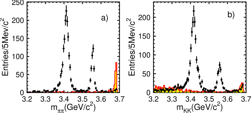
Figure 1: Invariant mass distributions of the two charged tracks in (a) $\gamma\pi^{+}\pi^{-}$ and (b) $\gamma K^{+}K^{-}$. Dots with error bars are data, and the shaded histograms are the MC simulated backgrounds.

Simulated background events passing the selection criteria for the $\gamma\pi^{+}\pi^{-}$ and $\gamma K^{+}K^{-}$ channels are also plotted in Fig. 1. The excess background in the $\gamma\pi^{+}\pi^{-}$ mode near 3.7 GeV/$c^{2}$ is due to the large $\psi(2S)\rightarrow\pi^{+}\pi^{-}$ branching ratio from the PDG pdg . The backgrounds under the signal regions are $\mu^{+}\mu^{-}(\gamma)$ and $e^{+}e^{-}(\gamma)$ events either from QED processes or from $\psi(2S)$ decays.

Requiring the invariant mass of the two charged tracks be between $3.54$ and $3.57$ GeV/$c^{2}$ to select $\chi_{c2}$, 418 $\gamma\pi^{+}\pi^{-}$ events and 303 $\gamma K^{+}K^{-}$ events are selected. The fractions of background are $(1.6\pm 0.5)\%$ for $\gamma\pi^{+}\pi^{-}$ and $(2.8\pm 0.6)\%$ for $\gamma K^{+}K^{-}$, as estimated from Monte Carlo simulation, in agreement with the expectation from the measured misidentification efficiencies in data.

Monte Carlo simulation also determines that the $K^{+}K^{-}$ contamination in the $\pi^{+}\pi^{-}$ sample is about 9%, and the $\pi^{+}\pi^{-}$ contamination in the $K^{+}K^{-}$ sample is about 34%. The effect of the cross contamination on the fit of the helicity amplitudes will be discussed later.

IV The Fit of the Helicity Amplitudes

The $\psi(2S)\to\gamma\chi_{c2}$ helicity amplitudes are determined by a maximum likelihood fit to the decay angular distribution 3161 ; 3065

$$W_{2}(\theta_{\gamma},\theta_{M},\phi_{M})={3x^{2}\sin^{2}\theta_{\gamma}\sin^{2}2\theta_{M}}+$$ (1)

$${(1+\cos^{2}\theta_{\gamma})[(3\cos^{2}\theta_{M}-1)^{2}+{\frac{3}{2}}y^{2}\sin^{4}\theta_{M}]}+$$

$${\sqrt{3}x\sin 2\theta_{\gamma}\sin 2\theta_{M}[3\cos^{2}\theta_{M}-1}-$$

$${{\frac{1}{2}\sqrt{6}}y\sin^{2}\theta_{M}]\cos\phi_{M}}$$

$${+\sqrt{6}y\sin^{2}\theta_{\gamma}\sin^{2}\theta_{M}(3\cos^{2}\theta_{M}-1)\cos 2\phi_{M}},$$

where $x=A_{1}/A_{0}$, $y=A_{2}/A_{0}$, $A_{0,1,2}$ are the $\chi_{c2}$ helicity amplitudes, $\theta_{\gamma}$ is the polar angle of the photon in the laboratory system, and $\theta_{M}$ and $\phi_{M}$ are the polar and azimuthal angles of one of the mesons in the $\chi_{c2}$ rest frame with respect to the $\gamma$ direction. $\phi_{M}=0$ is defined by the electron beam direction.

Fitting the $\gamma\pi^{+}\pi^{-}$ and $\gamma K^{+}K^{-}$ data, we obtain

$$x_{\pi} = 1.97\pm 0.64,\,\,y_{\pi}=3.03\pm 1.07,\,\,\rho_{\pi}=0.96,$$

$$x_{K} = 1.77\pm 0.54,\,\,y_{K}=2.36\pm 0.82,\,\,\rho_{K}=0.94,$$

where the errors are statistical and $\rho_{\pi}$, $\rho_{K}$ are the correlation factors between $x$ and $y$ for $\gamma\pi^{+}\pi^{-}$ and $\gamma K^{+}K^{-}$, respectively. The comparison between data and the fit is shown in Fig. 2. Good agreement is observed in all angular distributions for both the $\gamma\pi^{+}\pi^{-}$ and $\gamma K^{+}K^{-}$ channels.

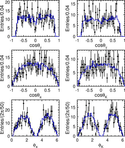
Figure 2: Comparison between data and the final fit for $\gamma\pi^{+}\pi^{-}$(left) and $\gamma K^{+}K^{-}$ (right), where dots with error bars are data and the histograms are the fit.

Since the value of the likelihood function does not provide a measurement of the goodness of fit, Pearson’s $\chi^{2}$ test is used. The data are divided into $3\times 3\times 4=36$ bins in $\cos\theta_{\gamma}$, $\cos\theta_{M}$ and $\phi_{M}$. The $\chi^{2}$ is calculated using

$$\chi^{2}=\sum\limits_{i}\frac{(n_{i}^{DT}-n_{i}^{MC})^{2}}{n_{i}^{DT}},$$

where $n_{i}^{DT}$ is the observed number of events in the $i$th bin and $n_{i}^{MC}$ is the corresponding number of events predicted by Monte Carlo using $x$ and $y$ fixed to the values determined in this analysis. We obtain $\chi_{\pi}^{2}/ndf=30.19/35=0.86$ and $\chi_{K}^{2}/ndf=43.57/35=1.24$ for the $\gamma\pi^{+}\pi^{-}$ and $\gamma K^{+}K^{-}$ channels, respectively, where $ndf$ is the number of the degree of freedom. These results show that the fits are good.

V Error analysis

V.1 Input output checking

The fitting procedure is tested using Monte Carlo simulated samples. With input parameters $x_{in}=\sqrt{3}\approx 1.732$ and $y_{in}=\sqrt{6}\approx 2.449$, fitting a Monte Carlo sample of 50,000 selected events gives the results $x_{out}=1.74\pm 0.04$, $y_{out}=2.45\pm 0.07$, and $\rho=0.94$, which are in good agreement with the input values, indicating the validity of the fitting procedure.

Dividing the 50,000 events into 100 subsets of 500 events each (about the same size as the real data sample) gives the distribution of fitting results shown in Fig. 3. $x$ and $y$ are positively correlated, and the fitting results are distributed in a relatively broad area due to the limited statistics of the subsets.

Figure 3: Distribution of fitting results for $x$ and $y$ for Monte Carlo simulated samples. The black dot with error bar is the result for all 50,000 events. The circles are the fitting results for the subsets after dividing the sample into 100 subsets.

V.2 Systematic errors

Systematic errors from background, from the $\gamma\pi^{+}\pi^{-}$ and $\gamma K^{+}K^{-}$ cross contamination, from the Monte Carlo simulation of the detector response, etc. are considered.

V.2.1 Background contamination

Backgrounds remaining after event selection are $\mu^{+}\mu^{-}(\gamma)$ and $e^{+}e^{-}(\gamma)$ events, and the fractions of backgrounds in $\gamma\pi^{+}\pi^{-}$ and $\gamma K^{+}K^{-}$ channels are estimated by Monte Carlo simulation and checked with data. In the fit, background is not considered, but the effect on the helicity amplitudes is estimated using Monte Carlo simulation. By adding the amount of MC background mentioned in Sec. III into the pure MC sample, the fit yields shifts of the fit results. These shifts are taken as corrections to the results obtained from data. By varying the background fraction in the fit, the uncertainty due to the background contamination can also be determined. It is found that the corrections to the $\gamma\pi^{+}\pi^{-}$ results are $\Delta_{\pi x}=0.19\pm 0.04$, $\Delta_{\pi y}=0.34\pm 0.07$; and for $\gamma K^{+}K^{-}$, $\Delta_{Kx}=0.25\pm 0.04$, $\Delta_{Ky}=0.47\pm 0.08$.

V.2.2 $\gamma\pi^{+}\pi^{-}$ and $\gamma K^{+}K^{-}$ cross contamination

In order to study the error from $\gamma\pi^{+}\pi^{-}$ and $\gamma K^{+}K^{-}$ cross contamination, Monte Carlo samples of $\gamma\pi^{+}\pi^{-}$ and $\gamma K^{+}K^{-}$ with $x=\sqrt{3}$, $y=\sqrt{6}$ are generated and mixed according to the amount of cross contamination determined by Monte Carlo simulation. It is found that the results from this mixed sample are mostly unchanged from those of the pure Monte Carlo sample, even when the contamination is doubled. This is understandable since the angular distributions of $\gamma\pi^{+}\pi^{-}$ and $\gamma K^{+}K^{-}$ are identical. From the comparisons of many Monte Carlo samples with different fractions of cross contamination, the errors on $x$ and $y$ are determined to be $0.01$ and $0.06$ for $x_{\pi}$ and $y_{\pi}$, and $0.10$ and $0.14$ for $x_{K}$ and $y_{K}$, respectively.

V.2.3 MC simulation of the detector response

The consistency between data and the Monte Carlo simulation of the detector response for $\chi_{c2}$ events can be determined using $\chi_{c0}$ events, although the absolute angular distributions are different. The angular distribution of $\chi_{c0}$ decays is unambiguous, i.e. $W_{0}=1+\cos^{2}\theta_{\gamma}$. Note that Eq. 1 with the $(3\cos^{2}\theta_{M}-1)$ term replaced by 1 is equal to $W_{0}$ when both $x$ and $y$ are zero. Therefore, if we fit the angular distribution of $\chi_{c0}$ the same as $\chi_{c2}$ using the modified Eq. 1, $x$ and $y$ should be 0. The difference from zero gives the systematic error due to the MC simulation of the detector response. For the $\gamma\pi^{+}\pi^{-}$ channel, 0.18, 0.05, and 0.24 are obtained for $x_{\pi}$, $y_{\pi}$ and $\rho_{\pi}$, respectively, and for the $\gamma K^{+}K^{-}$ channel, 0.13, 0.08, and -0.24 are obtained for $x_{K}$, $y_{K}$ and $\rho_{K}$. The results are dominated by the statistical errors of the fit due to the limited $\chi_{c0}$ samples, although they are already much larger than the corresponding $\chi_{c2}$ samples. Comparisons between data and Monte Carlo simulation for $\chi_{c0}$ events are shown in Fig. 4; good agreement is observed.

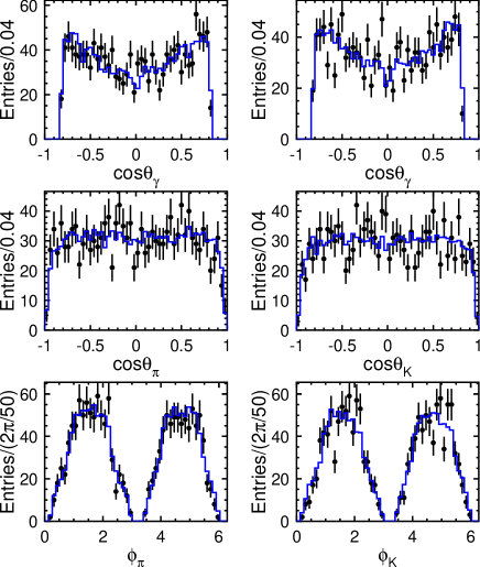
Figure 4: Comparison of angular distributions between data (dots with error bars) and Monte Carlo simulation (histograms) for $\chi_{c0}\rightarrow\pi^{+}\pi^{-}$ (left) and $\chi_{c0}\rightarrow K^{+}K^{-}$ (right). Fitting the $\chi_{c0}$ angular distributions provides a way to estimate the systematic error due to the Monte Carlo simulation of the detector response.

V.2.4 Other sources

Other sources of error are from systematic errors associated with the simulation of the mass resolution of the $\chi_{c2}$, the photon detection efficiency, the MDC tracking efficiency, the kinematic fit, the total number of the $\psi(2S)$ events, the trigger efficiency, etc. These systematic errors will affect a branching ratio measurement, but will not affect the measurement of the angular distribution. Their effects on the helicity amplitude measurements are neglected.

V.2.5 Total systematic error

The systematic errors and the correlation factors from all the above sources are listed in Table 1. Here the correlation factors ($\rho_{\pi}$ and $\rho_{K}$) from background contamination and $\gamma\pi^{+}\pi^{-}$ and $\gamma K^{+}K^{-}$ cross contamination are set to $1$, and the total correlation factor $\rho$ is calculated with $\rho=\Sigma_{i}\frac{\rho_{i}\sigma_{xi}\sigma_{yi}}{\sigma_{x}\sigma_{y}}$, where $i$ runs over all the systematic errors. The total systematic errors are $0.19$ and $0.11$ for $x$ and $y$ in $\gamma\pi^{+}\pi^{-}$ and $0.17$ and $0.18$ in $\gamma K^{+}K^{-}$.

Table 1: Summary of the systematic errors and correlations.

Source	$x_{\pi}$	$y_{\pi}$	$\rho_{\pi}$	$x_{K}$	$y_{K}$	$\rho_{K}$
Background contamination	$0.04$	$0.07$	1	$0.04$	$0.08$	1
$\pi/K$ cross contamination	$0.01$	$0.06$	1	$0.10$	$0.14$	1
MC simulation	$0.18$	$0.05$	0.24	$0.13$	$0.08$	-0.24
Total	$0.19$	$0.11$	0.29	$0.17$	$0.18$	0.49

VI Results and Discussion

After applying the corrections due to the background contamination, we obtain

$$x_{\pi} = 2.16\pm 0.64\pm 0.19,$$

$$y_{\pi} = 3.37\pm 1.07\pm 0.11,$$

$$\rho_{\pi}^{stat} = 0.96,\,\,\,\,\rho_{\pi}^{sys}=0.29$$

from $\gamma\pi^{+}\pi^{-}$ and

$$x_{K} = 2.02\pm 0.54\pm 0.17,$$

$$y_{K} = 2.83\pm 0.82\pm 0.18,$$

$$\rho_{K}^{stat} = 0.94,\,\,\,\,\rho_{K}^{sys}=0.49$$

from $\gamma K^{+}K^{-}$, where the first errors are statistical and the second are systematic, and $\rho^{stat}$ and $\rho^{sys}$ are the correlation factors between $x$ and $y$ of the statistical and systematic errors.

Combining the statistical and systematic errors yields:

$$x_{\pi} = 2.16\pm 0.67,\,\,y_{\pi}=3.37\pm 1.08,\,\,\rho_{\pi}=0.93,$$

$$x_{K} = 2.02\pm 0.57,\,\,y_{K}=2.83\pm 0.84,\,\,\rho_{K}=0.91.$$

The results from $\gamma\pi^{+}\pi^{-}$ and $\gamma K^{+}K^{-}$ are in good agreement. Combining them, we obtain

$$x = 2.08\pm 0.44,$$

$$y = 3.03\pm 0.66,$$

$$\rho = 0.92.$$

The combination assumes no correlation between $\gamma\pi^{+}\pi^{-}$ and $\gamma K^{+}K^{-}$ for both statistical and systematic errors.

Comparing with the measurement obtained by the Crystal Ball Cball , $a_{2}^{\prime}(\psi^{\prime}\to\gamma\chi)=0.132^{+0.098}_{-0.075}$, this measurement gives the quadrapole amplitude $a_{2}^{\prime}=-0.051^{+0.054}_{-0.036}$ and the octupole amplitude $a_{3}^{\prime}=-0.027^{+0.043}_{-0.029}$ amplitudes . Neither result significantly differs from zero. The results are in good agreement with what is expected for a pure $E1$ transition. As for the D-state mixing of $\psi(2S)$, our results do not contradict the previous theoretical calculation within one standard deviation PRD30p1924 .

VII Summary

The helicity amplitudes of $\psi(2S)\rightarrow\gamma\chi_{c2}$ are measured for $\chi_{c2}\rightarrow\pi^{+}\pi^{-}$ and $K^{+}K^{-}$, and $x=2.08\pm 0.44$, $y=3.03\pm 0.66$ with correlation $\rho=0.92$ are obtained. The results are in good agreement with a pure $E1$ transition, but still do not have the precision to strongly limit the higher multipoles.

References

(1) M. A. Doncheski et al., Phys. Rev. D 42, 2293 (1990).
(2) E. Eichten et al., Phys. Rev. D 21, 203 (1980).
(3) K. J. Sebastian, Phys. Rev. D 26, 2295 (1982).
(4) G. Hardekopf and J. Sucher, Phys. Rev. D 25,
2938 (1982).
(5) R. McClary and N. Byers, Phys. Rev. D 28,
1692 (1983).
(6) P. Moxhay and J. L. Rosner, Phys. Rev. D 28,
1132 (1983).
(7)J. L. Rosner, Phys. Rev. D 64, 094002 (2001);
P. Wang, X. H. Mo and C. Z. Yuan, Phys. Lett. B 574, 41
(2003).
(8)P. Wang, X. H. Mo and C. Z. Yuan,
hep-ph/0402227, Phys. Rev. D, in press.
(9) M. Oreglia et al., Phys. Rev. D 25, 2259
(1982).
(10)X. H. Mo et al. High Energy Physics and Nuclear
Physics 27, 455 (2004), hep-ex/0407055.
(11) J. Z. Bai. et al. (BES Collab.), Nucl. Instr.
Meth. A 344, 319 (1994).
(12) J. Z. Bai. et al. (BES Collab.), Nucl. Instr.
Meth. A 458, 627 (2001).
(13) J. Z. Bai. et al. (BES Collab.), High Energy
Physics and Nuclear Physics 20, 97 (1996) (in Chinese); and
Phys. Rev. D 58, 092006 (1998).
(14) S. Eidelman et al. (Particle Data Group),
Phys. Lett. B 592, 1 (2004).
(15) P. K. Kabir et al., Phys. Rev. D 13, 3161
(1976).
(16) C. Edwards et al., Phys. Rev. D 25, 3065
(1981).
(17) For the amplitude calculation formulas,
see G. Karl, S. Meshkov and J. L. Rosner, Phys. Rev. D 13,
1203 (1976).
(18) H. Grotch et al., Phys. Rev. D 30,
1924 (1984).