Max-Planck-Institut für Physik

JADE Note 146

MPP-2004-99

August 6, 2004

Measurement of the Strong Coupling Constant $\alpha_{\mathrm{S}}$ from the Four-Jet Rate in $\mathrm{e^{+}e^{-}}$ Annihilation using JADE data

J. Schieck, S. Kluth, S. Bethke, P.A. Movilla Fernandez, C. Pahl, and the JADE Collaboration

Data from $\mathrm{e^{+}e^{-}}$ annihilation into hadrons collected by the JADE experiment at centre-of-mass energies between 14 GeV and 44 GeV were used to study the four-jet rate as a function of the Durham algorithm’s resolution parameter $y_{\mathrm{cut}}$. The four-jet rate was compared to a QCD NLO order calculations including NLLA resummation of large logarithms. The strong coupling constant measured from the four-jet rate is

$\alpha_{\mathrm{S}}(M_{\mathrm{Z^{0}}})=0.1169\pm 0.0004\mathrm{(stat.)}\pm 0.0012\mathrm{(exp.)}\pm 0.0021\mathrm{(had.)}\pm 0.0007\mathrm{(theo.)}$,

$\alpha_{\mathrm{S}}(M_{\mathrm{Z^{0}}})=0.1169\pm 0.0026~{}(\mathrm{total~{}error})$

in agreement with the world average.

This note describes preliminary JADE results

1 Introduction

The annihilation of an electron and a positron into hadrons allows precise tests of Quantum Chromodynamics (QCD). Multijet rates are predicted in perturbation theory as functions of the jet-resolution parameter with one free parameter, the strong coupling constant $\alpha_{\mathrm{S}}$. Events with four quarks or two quarks and two gluons in the partonic final state are expected to lead predominantly to events with four jets in the observed hadronic final state. Thus, a determination of the four-jet production rate in hadronic events and fitting the theoretical prediction to the data provides a means to measure the strong coupling constant.

Calculations beyond leading order are made possible by theoretical developments achieved in the last few years. For multi-jet rates as well as numerous event shape distributions with perturbative expansions starting at $\cal{O}(\alpha_{\mathrm{S}})$, matched next-to-leading order calculations (NLO) and next-to-leading logarithmic approximations (NLLA) promise precise description of the data over a wide range of the available kinematic region and centre-of-mass energy [2, 3, 4, 5].

In this analysis we used data collected by the JADE experiment in the years 1979 to 1986 at the PETRA $\mathrm{e^{+}e^{-}}$ collider at DESY at six centre-of-mass energies covering the range of 14–44 GeV. Evidence for four-jet structure has been reported earlier by JADE [6]. In a previous OPAL publication a simultaneous measurement of $\alpha_{\mathrm{S}}$ and the QCD colour factors with data taken at $\sqrt{s}=91$ GeV is described [7]. The same theoretical predictions were used for this analysis, with the colour factors $C_{\mathrm{A}}$ and $C_{\mathrm{F}}$ set to the values expected from the QCD SU(3) symmetry group. A similar analysis was performed by ALEPH using LEP 1 data at $\sqrt{s}=91$ GeV [8].

The outline of the note is as follows. In section 2, we define the observable used in the analysis and describe its best available perturbative predictions. In section 3 the analysis procedure is explained in detail. Section 4 contains the discussion of the systematic checks which were performed and the resulting systematic errors. We collect our results in section 5 and summarize them in section 6.

2 Observable

Jet algorithms are applied to cluster the large number of particles of an hadronic event into a small number of jets, reflecting the parton structure of the event. For this analysis we used the Durham scheme [2]. Defining each particle initially to be a jet, a resolution variable $y_{ij}$ is calculated for each pair of jets $i$ and $j$:

$$y_{ij}=\frac{2\mathrm{min}(E_{i}^{2},E_{j}^{2})}{E_{\mathrm{vis}}^{2}}(1-\cos\theta_{ij}),$$ (1)

where $E_{i}$ and $E_{j}$ are the energies, $\cos\theta_{ij}$ is the angle between the two jets and $E_{\mathrm{vis}}$ is the sum of the energies of all visible particles in the event (or the partons in a theoretical calculation). If the smallest value of $y_{ij}$ is less than a predefined value $y_{\mathrm{cut}}$, the pair is replaced by a jet with four momentum $p_{ij}^{\mu}=p_{i}^{\mu}+p_{j}^{\mu}$, and the clustering starts again with $p_{ij}^{\mu}$ instead of the momenta $p_{i}^{\mu}$ and $p_{j}^{\mu}$. Clustering ends when the smallest value of $y_{ij}$ is larger than $y_{\mathrm{cut}}$. The remaining jets are then counted.

In QCD the fraction of four-jet events $R_{4}$ is predicted in NLO as a function of the strong coupling constant $\alpha_{\mathrm{S}}$. The prediction used here was given by [5]:

$$R_{4}(y_{\mathrm{cut}})=\frac{\sigma_{\mathrm{\mbox{\scriptsize{4-jet}}}}(y_{\mathrm{cut}})}{\sigma_{\mathrm{tot}}}\\ =\eta^{2}B_{4}(y_{\mathrm{cut}})+\eta^{3}[C_{4}(y_{\mathrm{cut}})+\frac{3}{2}(\beta_{0}\log{x_{\mu}}-1)\ B_{4}(y_{\mathrm{cut}})]$$ (2)

with $\sigma_{\mathrm{tot}}$ the total hadronic cross-section, $\eta=\alpha_{\mathrm{S}}C_{\mathrm{F}}/(2\pi)$, $x_{\mu}=\mu/\sqrt{s}$ with $\mu$ the renormalization scale and $\sqrt{s}$ the centre-of-mass energy, $\beta_{0}=(11-2n_{\mathrm{f}}/3)$ with $n_{\mathrm{f}}$ the number of active flavours. The coefficients $B_{4}$ and $C_{4}$ were obtained by integrating the matrix elements for $\mathrm{e^{+}e^{-}}$ annihilation into four massless parton final states, calculated by the program DEBRECEN 2.0 [5] . Eq. 2 is used to predict the four-jet rate as a function of $y_{\mathrm{cut}}$. The fixed-order perturbative prediction is not reliable for small values of $y_{\mathrm{cut}}$, due to terms $\sim\alpha_{\mathrm{S}}^{n}\ln^{m}(y_{\mathrm{cut}})$ that enhance the higher order corrections. An all-order resummation, given in [2], is possible for the Durham clustering algorithm. The NLLA calculation is combined with the NLO-prediction using the “modified R-matching” scheme described in [5]. In the modified R-matching scheme the terms proportional in $\eta^{2}$ and $\eta^{3}$ are removed from the $R^{\mathrm{NLLA}}$ prediction and the remainder is then added to the $R^{\mathrm{NLO}}$ calculation:

$$R^{\mathrm{R-match}}=R^{\mathrm{NLLA}}+[\eta^{2}(B_{4}-B^{\mathrm{NLLA}})+\eta^{3}(C_{4}-C^{\mathrm{NLLA}}-3/2(B_{4}-B^{\mathrm{NLLA}}))],$$ (3)

where $B^{\mathrm{NLLA}}$ and $C^{\mathrm{NLLA}}$ are the coefficients of the expansion of $R^{\mathrm{NLLA}}$ as in Eq. 2.

3 Analysis Procedure

3.1 The JADE Detector

A detailed description of the JADE detector can be found in [1]. This analysis relies mainly on the reconstruction of charged particle trajectories and on the measurement of energy deposited in the electromagnetic calorimeter. Tracking of charged particles was performed with the central detector, which was positioned in a solenoidal magnet providing an axial magnetic field of 0.48 T. The central detector contained a large volume jet chamber. Later a vertex chamber close to the interaction point and surrounding $z$-chambers to measure the $z$-coordinate  were added. Most of the tracking information was obtained from the jet chamber, which provided up to 48 measured space points per track, and good tracking efficiency in the region $|\cos\theta|<0.97$. Electromagnetic energy was measured by the lead glass calorimeter surrounding the magnet coil, separated into a barrel ($|\cos\theta|<0.839$) and two end-cap ($0.86<|\cos\theta|<0.97$) sections. The electromagnetic calorimeter consisted of 2520 lead glass blocks with a depth of 12.5 radiation lengths in the barrel (since 1983 increased to 15.7 in the middle 20% of the barrel) and 192 lead glass blocks with 9.6 radiation lengths in the end-caps.

3.2 Data Samples

The data used in this analysis were collected by JADE between 1979 and 1986 and correspond to a total integrated luminosity of 195 $\mathrm{pb}^{-1}$. The breakdown of the data samples, mean centre-of-mass energy, energy range, data taking period, collected integrated luminosities and the size of the data samples after selection of hadronic events are given in table 1. The data samples were chosen following previous analyses, e.g. [1, 9, 10, 11, 12]. The data are available from two versions of the reconstruction software from 9/87 and from 5/88. We used both sets and considered differences between the results as an experimental systematic uncertainty.

average	energy	year	luminosity	selected	selected
energy in GeV	range in GeV		($\mathrm{pb}^{-1}$)	events	events
				9/87	5/88
14.0	13.0–15.0	1981	1.46	1722	1783
22.0	21.0–23.0	1981	2.41	1383	1403
34.6	33.8–36.0	1981–1982	61.7	14213	14313
35.0	34.0–36.0	1986	92.3	20647	20876
38.3	37.3–39.3	1985	8.28	1584	1585
43.8	43.4–46.4	1984–1985	28.8	3896	4376

Table 1: The average center-of-mass energy, energy range, year of data taking and integrated luminosity for each data sample, together with the numbers of selected data events using the data sample version of 9/87 or 5/88.

3.3 Monte Carlo Samples

Samples of Monte Carlo simulated events were used to correct the data for experimental acceptance and backgrounds. The process $\mathrm{e^{+}e^{-}}\to\mathrm{hadrons}$ was simulated using PYTHIA 5.7 [13]. Corresponding samples using HERWIG 5.9 [14, 15] were used for systematic checks. The Monte Carlo samples generated at each energy point were processed through a full simulation of the JADE detector [21, 22, 23], summarized in  [12], and reconstructed in essentially the same way as the data.

In addition, for comparisons with the corrected data, and when correcting for the effects of fragmentation, large samples of Monte Carlo events without detector simulation were employed, using the parton shower models PYTHIA 6.158, HERWIG 6.2 and ARIADNE 4.11 [19]. All models were adjusted to LEP 1 data by the OPAL collaboration.

The ARIADNE Monte Carlo generator is based on a color dipole mechanism for the parton shower. The PYTHIA and HERWIG Monte Carlo programs use the leading logarithmic approximation (LLA) approach to model the emission of gluons in the parton shower. For the emission of the first hard gluon, the differences between the LLA approach and a leading order matrix element calculation are accounted for. However, the emission of gluons later on in the parton shower is based only on a LLA cascade and is expected to differ from a complete matrix element calculation. For this reason we do expect deviations in the description of the data by the Monte Carlo models. Recently new Monte Carlo generators have been developed, which implement a more complete simulation of the hard parton emission [20]. However, the models are not yet tuned to data taken at LEP and were therefore not considered in this analysis.

3.4 Selection of Events

The selection of events for this analysis aims to identify hadronic event candidates and to reject events with a large amount of energy emitted by initial state radiation (ISR). The selection of hadronic events was based on cuts on event multiplicity (to remove leptonic final states) and on visible energy and longitudinal momentum balance (to remove radiative and two-photon events, $\mathrm{e^{+}e^{-}}\to\mathrm{e^{+}e^{-}}$ hadrons). The cuts used are documented in [16, 17, 18] and summarized in a previous publication [9].

Standard criteria were used to select good tracks and clusters of energy deposits in the calorimeter for subsequent analysis. Charged particle tracks were required to have at least 20 hits in r-$\phi$ and at least 12 in r-$z$ in the jet chamber. The total momentum was required to be at least 50 MeV. Furthermore, the point of closest approach of the track to the collision axis was required to be less than 5 cm from the nominal collision point in the $x-y$ plane and less than 35 cm in the $z-$direction.

In order to mitigate the effects of double counting of energy from tracks and calorimeter clusters a standard algorithm was adopted which associated charged particles with calorimeter clusters, and subtracted the estimated contribution of the charged particles from the cluster energy. Charged particle tracks were assumed to be pions while the photon hypothesis was assigned to electromagnetic energy clusters. Clusters in the electromagnetic calorimeter were required to have an energy exceeding 0.15 GeV after the subtraction of the expected energy deposit of any associated tracks. From all accepted tracks and clusters $i$ the visible energy $E_{\mathrm{vis}}=\sum_{i}E_{i}$, momentum balance $p_{\mathrm{bal}}=|\sum_{i}p_{z,i}|/E_{\mathrm{vis}}$ and missing momentum $p_{\mathrm{miss}}=|\sum_{i}\vec{p}_{i}|$ were calculated. To charged particle tracks the pion mass was assigned while the mass of clusters was assumed to be zero.

Hadronic event candidates were required to pass the following selection criteria:

• The total energy deposited in the electromagnetic calorimeter had to exceed 1.2 GeV (0.2 GeV) for $\sqrt{s}<16$ GeV, 2.0 GeV (0.4 GeV) for $16<\sqrt{s}<24$ GeV and 3.0 GeV (0.4 GeV) for $\sqrt{s}>24$ GeV in the barrel (each endcap) of the detector.

• The number of good charged particle tracks was required to be greater than three reducing $\tau^{+}\tau^{-}$ and two-photon backgrounds to a negligible level.

• For events with exactly four tracks configurations with three tracks in one hemisphere and one track in the opposite hemisphere were rejected.

• At least three tracks had to have more than 24 hits in $r-\phi$ and a momentum larger than 500 MeV; these tracks are called long tracks.

• The visible energy had to fulfill $E_{\mathrm{vis}}/\sqrt{s}>0.5$.

• The momentum balance had to fulfill $p_{\mathrm{bal}}<0.4$.

• The missing momentum had to fulfill $p_{\mathrm{miss}}/\sqrt{s}<0.3$.

• The z-coordinate of the reconstructed event vertex had to lie within 15 cm of the interaction point.

• The polar angle of the thrust axis was required to satisfy $|\cos(\theta_{\mathrm{T}})|<0.8$ in order that the events be well contained in the detector acceptance.

The numbers of selected events for each $\sqrt{s}$ are shown in table 1 for the two versions of the data.

3.5 Corrections to the data

All selected tracks and the electromagnetic calorimeter clusters remaining after correcting for double counting of energy as described above were used in the evaluation of the four-jet rate. The four-jet rate distribution after all selection cuts had been applied is called the detector level distribution.

In this analysis events from the process $\mathrm{e^{+}e^{-}}\rightarrow\mathrm{b\bar{b}}$ were considered as background, since especially at low $\sqrt{s}$ the large mass of the b quarks and of the subsequently produced B hadrons will influence the four-jet rate distribution. The QCD predictions are calculated for massless quarks and thus we choose to correct our data for the presence of $\mathrm{b\bar{b}}$ events.

The expected number of $\mathrm{b\bar{b}}$ background events $\eta_{i}$ was subtracted from the observed number of data events $N_{i}$ at each $y_{\mathrm{cut}}$ point $i$. The effects of detector acceptance and resolution and of residual ISR were then accounted for by a multiplicative correction procedure.

Two four-jet rate distributions were formed from Monte Carlo simulated signal events; the first, at the detector level, treated the Monte Carlo events identically to the data, while the second, at the hadron level, was computed using the true momenta of the stable particles in the event, and was restricted to events where $\sqrt{s^{\prime}}$, the centre-of-mass energy reduced due to ISR, satisfied $\sqrt{s}-\sqrt{s^{\prime}}<0.15$ GeV. The Monte Carlo ratio of the hadron level to the detector level for each $y_{\mathrm{cut}}$ point $i$, $C^{\mathrm{detector}}_{i}$, was used as a correction factor for the data. This yields finally the corrected number of four jet events at $y_{\mathrm{cut}}$ point $i$ $\tilde{N_{i}}=C^{\mathrm{detector}}_{i}\cdot(N_{i}-\eta_{i})$. The hadron level distribution was then normalized at each $y_{\mathrm{cut}}$ point $i$ by calculating $R_{4,i}=\tilde{N_{i}}/N$, where $N$ is the expected total number of events.

The detector correction factors $C^{\mathrm{detector}}$ as determined using PYTHIA and HERWIG are shown in figure 1. We observe some disagreement between the detector corrections calculated using PYTHIA or HERWIG at low $\sqrt{s}$ while at larger $\sqrt{s}$ the correction factors agree well within the regions chosen for comparison with the theory predictions, see below. The difference in detector corrections was evaluated as an experimental systematic uncertainty.

A single event will usually contribute to several $y_{\mathrm{cut}}$ points in a four-jet rate distribution and for this reason the data points are correlated. The complete covariance matrix $W_{ij}$ was determined from four-jet rate distributions calculated at the hadron level in the following way. Subsamples were built by choosing 1000 events randomly out of the set of all generated Monte Carlo events. A single event can show up in several subsamples, but the impact on the final covariance matrix is expected to be very small and therefore was neglected. For every energy point 1000 subsamples were built. The covariance matrix was then used to determine the correlation matrix, $\rho_{ij}=W_{ij}/\tilde{\sigma_{i}}\tilde{\sigma_{j}}$, with $\tilde{\sigma_{i}}=\sqrt{W_{ii}}$.

The covariance matrix $V_{ij}$ used in the $\chi^{2}$ fit for the extraction of $\alpha_{\mathrm{S}}$ (see section 5.2 below) was then determined using the statistical error $\sigma_{i}$ of the data sample at $y_{\mathrm{cut}}$ point $i$ and the correlation matrix $\rho_{ij}$: $V_{ij}=\rho_{ij}\sigma_{i}\sigma_{j}$.

4 Systematic Uncertainties

Several sources of possible systematic uncertainties were studied. All systematic uncertainties were taken as symmetric. Contributions to the experimental uncertainties were estimated by repeating the analysis with varied cuts or procedures. For each systematic variation the value of $\alpha_{\mathrm{S}}$ was determined and then compared to the result of the standard analysis (default value). For each variation the difference with respect to the default value was taken as a systematic uncertainty. In the cases of two-sided systematic variations the larger deviation from the default value was taken as the systematic uncertainty.

• In the standard analysis the data version from 9/87 was used. As a variation a different data set from 5/88 was used.

• In the default method the tracks and clusters were associated and the estimated energy from the tracks was subtracted. As a variation all reconstructed tracks and all electromagnetic clusters were used.

• The thrust axis was required to satisfy $|\cos(\theta_{\mathrm{T}})|<0.7$. With this more stringent cut events were restricted to the barrel region of the detector, which provides better measurements of tracks and clusters compared to the endcaps.

• Instead of using PYTHIA for the correction of detector effects as described in section 3.5, events generated with HERWIG were used.

• The requirement on missing momentum was dropped or tightened to $p_{\mathrm{miss}}/\sqrt{s}<0.25$.

• The requirement on the momentum balance was dropped or tightened to $p_{\mathrm{bal}}<0.3$.

• The requirement on the number of long tracks was tightened to $N_{\mathrm{long}}\geq 4$.

• The requirement on the visible energy was varied to $E_{\mathrm{vis}}/\sqrt{s}>0.45$ and $E_{\mathrm{vis}}/\sqrt{s}>0.55$.

• The amount of subtracted $\mathrm{b\bar{b}}$ background was varied by $\pm$5% in order to cover uncertainties in the estimation of the background fraction in the data.

All contributions listed above were added in quadrature and the result quoted as the experimental systematic uncertainty. The dominating effects were the use of the different data version followed by employing HERWIG to determine the detector corrections. In the fits of the QCD predictions to the data two further systematic uncertainties were evaluated:

• The uncertainties associated with the hadronization correction (see section 5.2) were assessed by using HERWIG and ARIADNE instead of PYTHIA. The larger change in $\alpha_{\mathrm{S}}$ resulting from these alternatives was taken to define the hadronization systematic uncertainty.

• The theoretical uncertainty, associated with missing higher order terms in the theoretical prediction, was assessed by varying the renormalization scale factor $x_{\mu}$. The predictions of an all-orders QCD calculation would be independent of $x_{\mu}$, but a finite order calculation such as that used here retains some dependence on $x_{\mu}$. The renormalization scale $x_{\mu}$ was set to 0.5 and 2. The larger deviation from the default value was taken as theoretical systematic uncertainty.

5 Results

5.1 Four-Jet Rate Distributions

The four-jet rates for the six $\sqrt{s}$ points after subtraction of background and correction for detector effects are shown in figures 2 and 3. Superimposed are the distributions predicted by the PYTHIA, HERWIG and ARIADNE Monte Carlo models. In order to make a more clear comparison between data and models, the inserts in the upper right corner show the differences between data and each model, divided by the combined statistical and experimental error at that point. The sum of squares of these differences would, in the absence of point-to-point correlations, represent a $\chi^{2}$ between data and the model. However, since correlations are present, such $\chi^{2}$ values should be regarded only as a rough indication of the agreement between data and the models. The three models are seen to describe the data well.

5.2 Determination of $\alpha_{\mathrm{S}}$

Our measurement of the strong coupling constant $\alpha_{\mathrm{S}}$ is based on $\chi^{2}$ fits of QCD predictions to the corrected four-jet rate distribution, i.e. the data shown in figures 2 and 3. The theoretical predictions of the four-jet rate using the combined $\cal{O}(\alpha_{\mathrm{S}}^{\mathrm{3}})$+NLLA calculation as described in section 2 provide distributions at the parton level. In order to confront the theory with the hadron level data, it is necessary to correct for hadronization effects. The four-jet rate was calculated at hadron and parton level using PYTHIA and, as a cross-check, with the HERWIG and ARIADNE models. The theoretical prediction is then multiplied by the ratio $C^{\mathrm{had}}$ of the hadron and parton level four-jet rates to correct for hadronization.

The hadronization correction factors $C^{\mathrm{had}}$ as obtained from the three models are shown in figure 4. We find that the hadronization corrections reach values of down to about 0.5 at low $\sqrt{s}$ and there is a significant dependence on $y_{\mathrm{cut}}$. For larger $\sqrt{s}$ the hadronization corrections are closer to one as expected. We also observe that the models do not agree well at low $\sqrt{s}$. The differences between the models will be considered as a systematic uncertainty in the fits.

A $\chi^{2}$-value at each energy point is calculated using the following formula:

$$\chi^{2}=\sum_{i,j}^{n}(R_{4,i}-R(\alpha_{\mathrm{S}})_{4,i}^{\mathrm{theo}})(V_{ij})^{-1}(R_{4,j}-R(\alpha_{\mathrm{S}})_{4,j}^{\mathrm{theo}})$$ (4)

where the indices $i$ and $j$ denote the $y_{\mathrm{cut}}$ points in the chosen fit range and the $R(\alpha_{\mathrm{S}})_{4,i}^{\mathrm{theo}}$ are the predicted values of the four-jet rate. The covariance matrix is calculated as described in section 3.5. The $\chi^{2}$ value is minimized with respect to $\alpha_{\mathrm{S}}$ for each $\sqrt{s}$ separately. The scale parameter $x_{\mu}$, as discussed in section 2, is set to 1.

The fit ranges are shown in table 2. The fit ranges were determined by requiring that the detector hadronization corrections be less than $100\%$ in the fit region, and that the $\chi^{2}$/d.o.f. values changed by less than 2 units when one $y_{\mathrm{cut}}$ point is added to or removed from the fit range. The fit ranges cover the decreasing parts of the distributions at large $y_{\mathrm{cut}}$, where the perturbative QCD predictions are able to adequately describe the data corrected for hadronization. The increasing parts of the distributions at low $y_{\mathrm{cut}}$ are dominated by events with more than four jets which cannot be described accurately by the predictions. In addition experimental and hadronization corrections become large in this region.

In figures 5 and 6 the hadron level four-jet distributions for the six energy points are shown together with the fit result. The numerical results of the fits are summarized in table 3. The statistical error corresponds to the error from the $\chi^{2}$ minimization. The systematic errors were determined as described in section 4.

It is also of interest to combine the measurements of $\alpha_{\mathrm{S}}$ from the different centre-of-mass energy points in order to determine a single value. This problem has been subject of extensive study by the LEP QCD working group [24], and we adopt their procedure here.

In brief the method is as follows. The set of $\alpha_{\mathrm{S}}$ measurements to be combined are first evolved to a common scale, $Q=M_{\mathrm{Z^{0}}}$, assuming the validity of QCD. The measurements are then combined in a weighted mean, to minimize the $\chi^{2}$ between the combined values and the measurements. If the measured values evolved to $Q=M_{\mathrm{Z^{0}}}$ are denoted $\alpha_{\mathrm{S},i}$, with covariance matrix $V^{\prime}$, the combined values, $\alpha_{\mathrm{S}}(M_{\mathrm{Z^{0}}})$, are given by

$$\alpha_{\mathrm{S}}(M_{\mathrm{Z^{0}}})=\sum w_{i}\alpha_{\mathrm{S},i}\;\;\;\;\mathrm{where}\;\;\;\;w_{i}=\frac{\sum_{j}(V^{\prime~{}-1})_{ij}}{\sum_{j,k}(V^{\prime~{}-1})_{jk}},$$ (5)

where $i$ and $j$ denote the six individual results. The difficulty resides in making a reliable estimate of $V^{\prime}$ in the presence of dominant and highly correlated systematic errors. Small uncertainties in the estimation of these correlations can cause undesirable features such as negative weights. For this reason only experimental systematic errors assumed to be partially correlated between measurements were taken to contribute to the off-diagonal elements of the covariance matrix: $V^{\prime}_{ij}=\min(\sigma^{2}_{exp,i},\sigma^{2}_{exp,j})$. All error contributions (statistical, experimental, hadronization and scale uncertainty) were taken to contribute to the diagonal elements. The hadronization and scale uncertainties were computed by combining the $\alpha_{\mathrm{S}}$ values obtained with the alternative hadronization models, and from the upper and lower theoretical errors, using the weights derived from the covariance matrix $V^{\prime}$.

We find that the fit result from the 14 GeV data has large hadronization and experimental uncertainties because the corresponding corrections are large and not well known at this energy. We therefore choose to not include this result in the combination. The result of the combination using all results with $\sqrt{s}\geq 22$ GeV is

$$\alpha_{\mathrm{S}}(M_{\mathrm{Z^{0}}})=0.1169\pm 0.0004\mathrm{(stat.)}\pm 0.0012\mathrm{(exp.)}\pm 0.0021\mathrm{(had.)}\pm 0.0007\mathrm{(theo.)}\;,$$

consistent with the world average value of $\alpha_{\mathrm{S}}(M_{\mathrm{Z^{0}}})=0.1182\pm 0.0027$  [25]. The weights were 0.18 for 22 GeV, 0.29 for 34.6 GeV, 0.25 for 35 GeV, 0.07 for 38.3 GeV and 0.21 for 44 GeV. The results at each energy point are shown in figure 7 and compared with the predicted running of $\alpha_{\mathrm{S}}$ based on the world average value. For clarity the values from $\sqrt{s}=34.6$ and 35.0 GeV have been combined at their luminosity weighted average energy $\sqrt{s}=34.8$ GeV using the combination procedure described above. The result of ALEPH [8] and preliminary data from OPAL [26] are shown as well.

6 Summary

In this note we present preliminary measurements of the strong coupling from the four-jet rate at centre-of-mass energies between 14 and 44 GeV using data of the JADE experiment. The predictions of the PYTHIA, HERWIG and ARIADNE Monte Carlo models tuned by OPAL to LEP 1 data are found to be in agreement with the measured distributions.

From a fit of QCD NLO predictions combined with resummed NLLA calculations to the four-jet rate corrected for experimental and hadronization effects we have determined the strong coupling $\alpha_{\mathrm{S}}$. The value of $\alpha_{\mathrm{S}}(M_{\mathrm{Z^{0}}})$ is determined to be $\alpha_{\mathrm{S}}(M_{\mathrm{Z^{0}}})=0.1169\pm 0.0026~{}(\mathrm{total~{}error})$.

Tables

$\sqrt{s}$ [GeV]	fit range
14.0	0.00875 – 0.02765
22.0	0.0049 – 0.01555
34.6	0.0037 – 0.02765
35.0	0.0037 – 0.02765
38.3	0.0021 – 0.02765
43.8	0.0021 – 0.02075

Table 2: Fit ranges for all energy points

$\sqrt{s}$ [GeV]	$\alpha_{\mathrm{S}}(\sqrt{s})$	stat.	exp.	HERWIG	ARIADNE	$x_{\mu}=2.0$	$x_{\mu}=0.5$
14.0	0.1475	$\pm$0.0014	$\pm$0.0032	+0.0093	+0.0117	+0.0030	$-$0.0018
22.0	0.1442	$\pm$0.0018	$\pm$0.0028	$-$0.0005	+0.0038	+0.0018	$-$0.0002
34.6	0.1358	$\pm$0.0007	$\pm$0.0018	$-$0.0031	+0.0010	+0.0011	+0.0007
35.0	0.1405	$\pm$0.0006	$\pm$0.0017	$-$0.0033	+0.0009	+0.0012	+0.0008
38.3	0.1366	$\pm$0.0021	$\pm$0.0045	$-$0.0038	+0.0009	+0.0004	+0.0021
43.8	0.1303	$\pm$0.0012	$\pm$0.0011	$-$0.0038	+0.0005	+0.0001	+0.0020

Table 3: The value of $\alpha_{\mathrm{S}}$ for each energy point and the statistical, experimental, hadronization and scale errors.

Figures

Figure 1: The figures show the detector corrections for the four-jet rate at the six energy points as calculated using PYTHIA and HERWIG.

Figure 2: The figures show the four-jet rate distribution at hadron level as a function of the $y_{\mathrm{cut}}$ resolution parameter obtained with the Durham algorithm. The four-jet rate at five average centre-of-mass energies for the data, corrected to the hadron level, are shown for $\sqrt{s}=14$ to 35 GeV in comparison with predictions based on PYTHIA, HERWIG and ARIADNE Monte Carlo events. The errors shown include all statistical and experimental uncertainties. The panel in each upper right corner shows the differences between data and Monte Carlo, divided by the sum of the statistical and experimental error. At points with no data events, the difference is set to zero.

Figure 3: Same as figure 2 for $\sqrt{s}=38.3$ and 43.8 GeV.

Figure 4: The figures show the hadronization corrections for the four-jet rate at the six energy points as calculated using PYTHIA, HERWIG and ARIADNE.

Figure 5: The plots show the four-jet rate distributions at the hadron level for $\sqrt{s}=14$ GeV to 35 GeV. The errors correspond to the statistical error only and the curves indicate the theory prediction after using the fit results.

Figure 6: Same as figure 5 for $\sqrt{s}=38.3$ GeV and 43.8 GeV

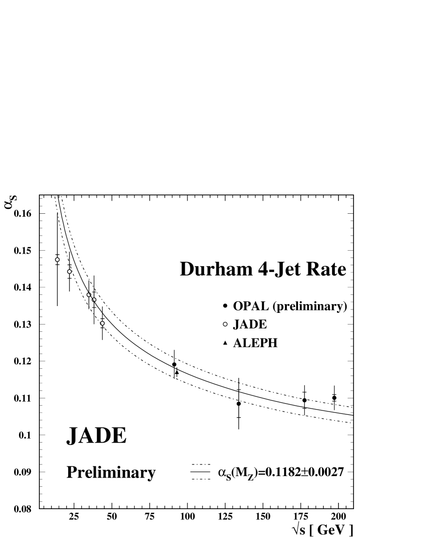
Figure 7: The values for $\alpha_{\mathrm{S}}$ at the various energy points. The errors show the statistical (inner part) and the total error. The full and dash-dotted lines indicate the current world average value of $\alpha_{\mathrm{S}}(M_{\mathrm{Z^{0}}})$ [25]. The results at $\sqrt{s}=34.6$ and 35 GeV have been combined for clarity. The results from ALEPH [8] and OPAL [26] (preliminary) are shown as well.

References

- [1] B. Naroska: Phys. Rep. 148 (1987) 67
- [2] S. Catani et al.: Phys. Lett. B 269 (1991) 432
- [3] L.J. Dixon, A. Signer: Phys. Rev. D 56 (1997) 4031
- [4] Z. Nagy, Z. Trocsanyi: Phys. Rev. D 57 (1998) 5793
-
[5]
Z. Nagy, Z. Trocsanyi: Phys. Rev. D 59 (1998) 014020,
Erratum-ibid.D62:099902,2000 - [6] JADE Coll., W. Bartel et al.: Phys. Lett. B 115 (1982) 338
- [7] OPAL Coll., G. Abbiendi et al.: Eur. Phys. J. C 20 (2001) 601
- [8] ALEPH Coll., A. Heister et al.: Eur. Phys. J. C 27 (2003) 1
- [9] JADE Coll., P.A. Movilla Fernández, O. Biebel, S. Bethke, S. Kluth, P. Pfeifenschneider et al.: Eur. Phys. J. C 1 (1998) 461
- [10] JADE and OPAL Coll., P. Pfeifenschneider et al.: Eur. Phys. J. C 17 (2000) 19
- [11] P.A. Movilla Fernández: In: ICHEP 2002: Parallel Sessions, S. Bentvelsen, P. de Jong, J. Koch, E. Laenen (eds.), 361. North-Holland, 2003
- [12] P.A. Movilla Fernández: Ph.D. thesis, RWTH Aachen, 2003, PITHA 03/01
- [13] T. Sjöstrand: Comput. Phys. Commun. 82 (1994) 74
- [14] G. Marchesini et al.: Comput. Phys. Commun. 67 (1992) 465
- [15] G. Corcella et al.: J. High Energy Phys. 01 (2001) 010
- [16] JADE Coll., W. Bartel et al.: Phys. Lee B88 (1979), 171.
- [17] JADE Coll., W. Bartel et al.: Phys. Lee B129 (1983), 145.
- [18] JADE Coll., S. Bethke et al.: Phys. Lee B213 (1988), 235.
- [19] L. Lönnblad: Comput. Phys. Commun. 71 (1992) 15
- [20] R. Kuhn, F. Krauss, B. Ivanyi, G. Soff: Comput. Phys. Commun. 134 (2001) 223
- [21] E. Elsen: Detector Monte Carlos, JADE Computer Note 54.
- [22] E. Elsen: Multihadronerzeugung in Vernichtung beu PETRA-Energien und Vergleich mit Aussagen der Quantenchromodynamic, PhD thesis, Universität Hamburg, 1981.
- [23] C. Bowdery and J. Olsen: The JADE SUPERVISOR Program, JADE Computer Note 73.
- [24] The LEP Experiments (ALEPH, DELPHI, L3 and OPAL) and the LEP QCD Working Group: paper in preparation
- [25] S. Bethke: MPP-2004-88, hep-ex/0407021 (2004)
- [26] OPAL Coll., G. Abbiendi et al.: OPAL physics note PN527 (2004), unpublished