Hadronic Branching Fractions of $D^{0}$ and $D^{+}$, and
$\sigma(e^{+}e^{-}\to D\bar{D}$) at $E_{\mathrm{cm}}=3.77$ GeV

Abstract

Using nearly 60 pb^-1 of data collected with the CLEO-c detector at the $\psi(3770)$ resonance, we measure absolute branching fractions for three $D^{0}$ and two $D^{+}$ Cabibbo-allowed hadronic decay modes, and the cross section for $e^{+}e^{-}\to D\bar{D}$ at $E_{\mathrm{cm}}=3.77$ GeV. We report preliminary measurements of the reference branching fractions, ${\cal B}(D^{0}\to K^{-}\pi^{+})=(3.92\pm 0.08\pm 0.23)\%$ and ${\cal B}(D^{+}\to K^{-}\pi^{+}\pi^{+})=(9.8\pm 0.4\pm 0.8)\%$, and preliminary measurements of other major branching fractions, ${\cal B}(D^{0}\to K^{-}\pi^{+}\pi^{0})=(14.3\pm 0.3\pm 1.0)\%$, ${\cal B}(D^{0}\to K^{-}\pi^{+}\pi^{+}\pi^{-})=(8.1\pm 0.2\pm 0.9)\%$, and ${\cal B}(D^{+}\to K^{0}_{S}\pi^{+})=(1.61\pm 0.08\pm 0.15)\%$. We determine preliminary values of the cross sections, $\sigma(e^{+}e^{-}\to D^{0}\bar{D}^{0})=(3.47\pm 0.07\pm 0.15)$ nb, $\sigma(e^{+}e^{-}\to D^{+}D^{-})=(2.59\pm 0.11\pm 0.11)$ nb, and $\sigma(e^{+}e^{-}\to D\bar{D})=(6.06\pm 0.13\pm 0.22)$ nb. We note that the Monte Carlo simulations used in calculating efficiencies in this analysis included final state radiation. However, the branching fractions used in the Particle Data Group averages do not include this effect. If we had not included final state radiation in our simulations, branching fractions would have been 0.5% to 2% lower.

I Introduction

We present preliminary absolute measurements of the Cabibbo-allowed $D^{0}$ and $D^{+}$ branching fractions, ${\cal B}(D^{0}\to K^{-}\pi^{+})$, ${\cal B}(D^{0}\to K^{-}\pi^{+}\pi^{0})$, ${\cal B}(D^{0}\to K^{-}\pi^{+}\pi^{+}\pi^{-})$, ${\cal B}(D^{+}\to K^{-}\pi^{+}\pi^{+})$, and ${\cal B}(D^{+}\to K^{0}_{S}\pi^{+})$. Two of these branching fractions, ${\cal B}(D^{0}\to K^{-}\pi^{+})$ and ${\cal B}(D^{+}\to K^{-}\pi^{+}\pi^{+})$, along with the branching fraction for $D_{s}^{+}\to\phi\pi^{+}$, are particularly important because essentially all other $D^{0}$, $D^{+}$, and $D_{s}^{+}$ branching fractions are determined from ratios to one or the other of these branching fractions PDG . As a result, nearly all branching fractions in the weak decay of heavy quarks are ultimately tied to one of these three branching fractions, called reference branching fractions in this paper. Furthermore, these reference branching fractions appear in many measurements of CKM matrix elements for $c$ and $b$ quark decay.

We note that the Monte Carlo simulations used in calculating efficiencies in this analysis included final state radiation. However, the branching fractions used in the Particle Data Group averages do not include this effect. If we had not included final state radiation in our simulations, the branching fractions we measure would have been 0.5% to 2% lower than they are.

II Branching Fractions and Production Cross Sections

The data for these measurements were obtained in $e^{+}e^{-}$ collisions at $E_{\mathrm{cm}}=3.77$ GeV, the peak of the $\psi(3770)$ resonance. At this energy, no additional hadrons accompany the $D^{0}\bar{D}^{0}$ and $D^{+}D^{-}$ pairs that are produced. These unique $D\bar{D}$ final states provide a powerful tool for addressing the most vexing problem in measuring absolute $D$ branching fractions at higher energies – the difficulty of accurately determining the number of $D$ mesons produced. Following the MARK III collaboration markiii-1 ; markiii-2 , reconstruction of one $D$ meson (called single tag or ST) serves to tag the event as either $D^{0}\bar{D}^{0}$ or $D^{+}D^{-}$. Branching fractions for $D^{0}$ or $D^{+}$ decay can then be obtained from the number of “double tag” (DT) events in which both the $D$ and the $\bar{D}$ are reconstructed, without knowledge of luminosity or the total number of $D\bar{D}$ events produced. Also, since $E_{\mathrm{cm}}$ is below threshold for production of $D_{s}^{+}D_{s}^{-}$, accurate absolute measurement of ${\cal B}(D_{s}^{+}\to\phi\pi^{+})$ using the techniques in this paper remains a challenge for the future.

If no distinctions are made between $D$ and $\bar{D}$ decays and their efficiencies, the number of ST events $N_{i}$ observed in the decay mode $i$ (and its charge conjugate) with branching fraction ${\cal B}_{i}$ and detection efficiency $\epsilon_{i}$ will be,

$$N_{i}=2N_{D\bar{D}}{\cal B}_{i}\epsilon_{i},$$

where $N_{D\bar{D}}$ is the number of $D\bar{D}$ events produced in the experiment. Then, the number of DT events with $D\bar{D}$ pairs reconstructed in modes $i$ and $j$ will be,

$$N_{ij}=2N_{D\bar{D}}{\cal B}_{i}{\cal B}_{j}\epsilon_{ij}~{}~{}(\mathrm{if}~{}i\neq j)\mathrm{~{}~{}or~{}~{}}N_{ii}=N_{D\bar{D}}{\cal B}_{i}^{2}\epsilon_{ii}~{}~{}(\mathrm{if}~{}i=j)$$

Hence, the ratios of DT events ($N_{ij}$) to ST events ($N_{j}$) provide absolute measurements of the branching fraction ${\cal B}_{i}$,

$${\cal B}_{i}={N_{ij}\over N_{j}}{\epsilon_{j}\over\epsilon_{ij}}\mathrm{~{}~{}or~{}~{}}{\cal B}_{i}={2N_{ii}\over N_{i}}{\epsilon_{i}\over\epsilon_{ii}}.$$

Note that $\epsilon_{ij}\approx\epsilon_{i}\epsilon_{j}$, so $\epsilon_{j}$ nearly cancels from the ratio $\epsilon_{j}/\epsilon_{ij}$. Hence, a branching fraction ${\cal B}_{i}$ obtained using this procedure is nearly independent of the efficiencies of tagging modes. Of course, ${\cal B}_{i}$ is sensitive to $\epsilon_{i}$ and its uncertainties.

Estimating errors and combining measurements using just these expressions is very difficult because $N_{ij}$ and $N_{j}$ are correlated (whether or not $i=j$) and measurements of ${\cal B}_{i}$ using different tagging modes $j$ are also correlated. To address this problem, we have developed a $\chi^{2}$ fitting procedure brfit which fits simultaneously all charged and neutral $D$ branching fractions and the numbers of charged and neutral $D\bar{D}$ pairs. Although the $D^{0}$ and $D^{+}$ branching fractions are statistically independent, systematic effects introduce significant correlations among them. Therefore, we fit both charged and neutral $D$ mesons simultaneously, and we include both statistical and systematic uncertainties, as well as their correlations, in the fit. We also perform corrections for backgrounds, efficiency, and crossfeed among modes directly in the fit, as the sizes of these adjustments depend on the fit parameters. Thus, all experimental measurements, such as event yields, efficiencies, and background branching fractions, are treated in a consistent manner. We actually fit $D$ and $\bar{D}$ yields separately in order to accommodate possible differences in efficiency, but charge conjugate branching fractions are constrained to be equal.

The number of $D\bar{D}$ events that were produced can be calculated from

$$N_{D\bar{D}}={N_{i}N_{j}\over 2N_{ij}}{\epsilon_{ij}\over\epsilon_{i}\epsilon_{j}}\mathrm{~{}~{}or~{}~{}}N_{D\bar{D}}={N_{i}^{2}\over 4N_{ii}}{\epsilon_{ii}\over\epsilon_{i}^{2}}.$$

The production cross sections for $D^{0}\bar{D}^{0}$ and $D^{+}D^{-}$ can then be obtained by combining $N_{D^{0}\bar{D}^{0}}$ and $N_{D^{+}D^{-}}$ – which are determined in the branching fraction fit – with the integrated luminosity ${\cal L}$. Note that $N_{D\bar{D}}$ obtained by this procedure is almost independent of the efficiencies.

Charge conjugate particles and decay modes are always implied in this paper unless stated otherwise.

III The CLEO-c Detector

The CLEO-c detector is a modification of the CLEO III detector cleoiidetector ; cleoiiidr ; cleorich in which the silicon-strip vertex detector was replaced with a six-layer vertex drift chamber, whose wires are all at small stereo angles to the beam axis cleocyb . The charged particle tracking system, consisting of the vertex drift chamber and a 47-layer central drift chamber cleoiiidr operates in a 1.0 T magnetic field, whose direction is along the beam axis. The momentum resolution achieved with the tracking system is $\sim 0.6$% at $p=1$ GeV/$c$. Photons are detected in an electromagnetic calorimeter consisting of about 8000 CsI(Tl) crystals cleoiidetector . The calorimeter attains a photon energy resolution of 2.2% at $E_{\gamma}=1$ GeV and 5% at 100 MeV. The solid angle coverage for charged and neutral particles of the CLEO-c detector is 93% of $4\pi$. We utilize two devices to obtain particle identification information to separate $K^{\pm}$ from $\pi^{\pm}$: the central drift chamber (which provides measurements of ionization energy loss – $dE/dx$) and a cylindrical ring-imaging Cherenkov (RICH) detector cleorich surrounding the central drift chamber. The solid angle of the RICH detector for separation of $K^{\pm}$ from $\pi^{\pm}$ is 80% of $4\pi$. The combined $dE/dx$-RICH particle identification procedure has a pion or kaon efficiency $>90$% and a probability of pions faking kaons (or vice versa) $<5$%.

The integrated luminosity ($\cal{L}$) of the data sets was measured using $\gamma\gamma$ events in the calorimeter lumins . Event counts were normalized with a Monte Carlo (MC) simulation based on the Babayaga bby event generator combined with GEANT-based geant detector modeling.

IV Data Sample and Event Selection

In this analysis, we utilized a total integrated luminosity of ${\cal L}=57.2\pm 1.7$  pb^-1 of $e^{+}e^{-}$ data collected at $E_{\mathrm{cm}}=3.77$ GeV. The data were produced with the Cornell Electron Storage Ring (CESR) operating in a new configuration cleocyb that includes six wiggler magnets to enhance synchrotron radiation damping at energies in the charm threshold region. Since these data were obtained, six additional wiggler magnets have been installed in CESR and future CESR operation in this energy region will be with the full complement of twelve wiggler magnets. The spread in $E_{\mathrm{cm}}$ with the six wiggler magnets is 2.3 MeV.

We reconstructed all events that satisfied the CLEO-c trigger and preserved them for further analyses. Most CLEO-c analyses of $D$ meson decays utilize a subset of the data in which each event contains at least one $D$ meson candidate selected by a standard set of requirements. This selection procedure begins with standardized requirements for $\pi^{\pm}$, $K^{\pm}$, $\pi^{0}$, and $K^{0}_{S}$ candidates.

Charged track candidates must pass the following quality requirements: the momentum of the track $p$ must be in the range $0.050\leq p\leq 2.0$ GeV/$c$, the track must pass within 0.5 cm of the origin in the $x$-$y$ plane (transverse to the beam direction), the track must pass within 5.0 cm of the origin in the $z$ direction, the polar angle $\theta$ was required to be in the range $|\cos\theta|<0.93$, and the number of hits reconstructed on the track was required to be at least half of the number of layers traversed by the track. Both requirements on the distance of the track from the origin of the coordinate system (which is close to the point where the two beams intersect) are approximately five times the standard deviation for the corresponding measurement.

We identified charged track candidates as pions or kaons using $dE/dx$ and RICH information. Each track was considered as both a potential $K^{\pm}$ and $\pi^{\pm}$ candidate. In the rare case that no useful information of either sort was available, we did not change this assignment.

If $dE/dx$ information was available, we calculate $\chi^{2}_{E}(\pi)$ and $\chi^{2}_{E}(K)$ from the $dE/dx$ measurements, the expected $dE/dx$ for pions and kaons of that momentum, and the appropriate standard deviations. We rejected tracks as kaon candidates when $\chi_{E}^{2}(K)$ was greater than 9, and similarly for pions. The difference $\chi^{2}_{E}(\pi)-\chi^{2}_{E}(K)$ was also calculated. If $dE/dx$ information was not available this $\chi^{2}$ difference was set equal to 0.

We used RICH information if the track momentum was sufficiently above the $K$ threshold ($p>0.55$ GeV/$c$), and the track was within the RICH acceptance ($|\cos\theta|<0.8$). We then rejected tracks as kaon candidates when the number of Cherenkov photons detected for the the kaon hypothesis was less than three, and similarly for pions. When there were at least three photons for the hypothesis under consideration, and information was available for both pion and kaon hypotheses, we calculated a $\chi^{2}$ difference for the RICH, $\chi^{2}_{R}(\pi)-\chi^{2}_{R}(K)$, from the locations of Cherenkov photons and the track parameters. Otherwise, we set this $\chi^{2}$ difference equal to 0.

Then we combined these $\chi^{2}$ differences in an overall $\chi^{2}$ difference, $\Delta\chi^{2}\equiv\chi^{2}_{E}(\pi)-\chi^{2}_{E}(K)+\chi^{2}_{R}(\pi)-\chi^{2}_{R}(K)$. If $\Delta\chi^{2}\leq 0$, we used the track as a pion candidate; If $\Delta\chi^{2}\geq 0$, we used the track as a kaon candidate.

We formed neutral pion candidates from pairs of photons, each of whose energy was greater than 30 MeV and whose showers pass photon quality requirements. An unconstrained mass $M(\gamma\gamma)$ was calculated from the energies and momenta of the two photons. This mass was required to be within $3\sigma$ with a nominal $\pi^{0}$ mass value which varied slightly with the total momentum of the $\pi^{0}$ candidate. The energy and momentum obtained from a kinematic fit of the two photon candidates to the mass $M_{\pi^{0}}$ from the PDG PDG was then used in further analysis.

We built $K^{0}_{S}$ candidates from pairs of tracks that intersect a vertex. We then subjected the tracks to a constrained vertex fit and used the resulting track parameters to calculate the invariant mass, $M(\pi^{+}\pi^{-})$. We called the track pair a $K^{0}_{S}$ candidate if the invariant mass $M(\pi^{+}\pi^{-})$ was within $3\sigma$, with $\sigma=4$ MeV/$c^{2}$, of the mass $M_{K^{0}}$ from the PDG PDG .

After event reconstruction, the next major step was selecting $D\bar{D}$ events with relatively loose requirements for further analysis. In this CLEO-c standard selection process we reconstructed $D^{0}$ candidates in 18 important decay modes and $D^{+}$ candidates in 6 important decay modes, although only three $D^{0}$ modes and two $D^{+}$ modes were used in this analysis. Two requirements were placed on $D^{0}$ and $D^{+}$ candidates formed from $\pi^{\pm}$, $K^{\pm}$, $\pi^{0}$ and $K^{0}_{S}$ candidates selected using the requirements described above. We calculate the energy difference, $\Delta E\equiv E(D)-E_{0}$, where $E(D)$ is the total energy of the particles in the $D$ candidate and $E_{0}$ is the energy of the $e^{\pm}$ beams. We accept candidates for further analysis if $|\Delta E|<100$ MeV. We calculate the mass of the $D$ candidate $M(D)$ by substituting the beam energy $E_{0}$ for the energy $E(D)$ of the $D$ candidate, i.e., $M^{2}(D)c^{4}\equiv E_{0}^{2}-p^{2}(D)c^{2}$, where $p(D)$ is the total momentum of the particles in the $D$ candidate. Then we required $M(D)>1.83$ GeV/$c^{2}$ to retain a $D$ candidate for further analysis. We included all events with $D$ candidates in any of the 24 decay modes that satisfied these loose requirements.

For the analysis described in this paper, we restricted our attention to the five decay modes mentioned previously, and we refined the requirements for acceptable $D$ candidates that were described in the previous paragraph. First, we used the more restrictive requirements on $|\Delta E|$, given in Table 1 that were tailored for each individual decay mode. For the ST analysis, we chose the candidate with the smallest $|\Delta E|$, if there was more than one $D$ candidate in a particular mode. Multiple candidates were rare in all modes except $D^{0}\to K^{-}\pi^{+}\pi^{0}$ where approximately 15% of the events had multiple candidates. In events with only two charged tracks that were consistent with our requirements for $D^{0}\to K^{-}\pi^{+}$ decays, we also imposed additional requirements to eliminate $e^{+}e^{-}\to e^{+}e^{-}$ and $e^{+}e^{-}\to\mu^{+}\mu^{-}$ events. Since we are not considering any all-neutral modes in this analysis, these requirements only affect ST yields, i.e., we would not try to find DT candidates with the $D$ or $\bar{D}$ decaying in an all neutral mode recoiling from a $D^{0}\to K^{-}\pi^{+}$ candidate.

Table 1: Requirements on $\Delta E$ for $D$ candidates accepted for the final analysis. The limits are set at approximately $3\sigma$.

Mode	Requirement (MeV)
$D^{0}\to K^{-}\pi^{+}$	$|\Delta E|<29.4$
$D^{0}\to K^{-}\pi^{+}\pi^{0}$	$-58.3<\Delta E<35.0$
$D^{0}\to K^{-}\pi^{+}\pi^{+}\pi^{-}$	$|\Delta E|<20.0$
$D^{+}\to K^{-}\pi^{+}\pi^{+}$	$|\Delta E|<21.8$
$D^{+}\to K^{0}_{S}\pi^{+}$	$|\Delta E|<26.5$

To obtain $D\bar{D}$ events for DT yields, we select only one candidate per event per combination $D$ and $\bar{D}$ decay modes. We apply the $\Delta E$ requirements described for the ST analyses, but do not choose the best candidate on the basis of minimum $|\Delta E|$. Instead, we choose the combination with the average of $M(D)$ and $M(\bar{D})$ – i.e., $\widehat{M}(D)\equiv[M(D)+M(\bar{D})]/2$ – closest to $M_{D}$. In careful studies of Monte Carlo events, we demonstrated that this procedure does not generate false peaks at the $D$ mass in the $M(D)$ vs. $M(\bar{D})$ distributions that are narrow enough or large enough to be confused with the DT signal.

V Generation and Study of Monte Carlo Events

We used Monte Carlo simulations to develop the procedures for measuring branching fractions and production cross sections, to understand the response of the CLEO-c detector, to determine parameters to use in fits to determine data yields, and to estimate and understand possible backgrounds. In each case $e^{+}e^{-}\to\psi(3770)\to D\bar{D}$ events were generated with the EvtGen program evtgen , and the response of the detector to the daughters of the $D\bar{D}$ decays was simulated with GEANT geant . The EvtGen program includes simulation of initial state radiation (ISR) – radiation of a photon by the $e^{+}$ and/or $e^{-}$ before their annihilation. The program PHOTOS photos was used to simulate final state radiation (FSR) – radiation of photons by the charged particles in the final state. We simulated two types of $D$ meson decays:

• signal Monte Carlo decays, in which a $D$ or a $\bar{D}$ decays in one of the 5 modes measured in this analysis, and

• generic Monte Carlo decays, in which a $D$ or $\bar{D}$ decays in accord with decay modes and branching fractions based on the 2002 Particle Data Group compilation pdg2002 . (Some tuning was required to match inclusive distributions in data.)

Using these two types of simulated decays, we generated three types of Monte Carlo events:

• generic Monte Carlo events, in which both the $D$ and the $\bar{D}$ decay generically,

• single tag signal Monte Carlo events, in which either the $D$ or the $\bar{D}$ always decays in one of the 5 modes measured in this analysis while the $\bar{D}$ or $D$, respectively, decays generically, and

• double tag signal Monte Carlo events, in which both the $D$ and the $\bar{D}$ decay in one of the 5 modes in this analysis.

Our signal Monte Carlo events included simulations of ISR, but our generic Monte Carlo events were generated before ISR was included in the simulations. The roles played by these Monte Carlo samples are described below.

We applied the same selection criteria for $D$ candidates and $D\bar{D}$ events in analyzing data and Monte Carlo events. We compared many distributions of particle kinematical quantities in data and Monte Carlo events to asses the accuracy and reliability of the Monte Carlo simulation of event generation and detector response. The agreement between data and Monte Carlo events for both charged and neutral particles was excellent for nearly all distributions of kinematic variables that we studied. The results of this analysis are not sensitive to the modest discrepancies that were observed in a few distributions.

VI Single Tag Efficiencies and Data Yields

We used binned likelihood fits to ST $M(D)$ distributions in Monte Carlo events to determine experimental resolutions and ST efficiencies. We then used some of these experimental resolution parameters in binned likelihood fits to data to determine ST data yields. Four probability distribution functions were used in fits to ST data and ST Monte Carlo events:

• Fits to mass ($m=M(D)$) distributions in ST Monte Carlo events without ISR used a relatively narrow core Gaussian $g(m;\mu,\sigma)$ to account for beam energy spread and a small contribution from detector resolution. The mean $\mu$, standard deviation $\sigma$, and area $A$ of the core Gaussian were among the parameters determined in the fits.

• In fits to Monte Carlo events with ISR and to data, the core Gaussian function was replaced by an inverted Crystal Ball cbf function $c(m;\mu,\sigma,\alpha,n)$ to account for the radiative tail on the high mass side of the peak due to ISR. This function is identical to $g(m;\mu,\sigma)$ for $m<\mu+\alpha\sigma$, but for larger values of $m$ the Gaussian is replaced with a radiative tail function that depends on $\alpha$ and $n$. The parameters $\alpha$ and $n$ are determined by fits to the mass distributions.

• All fits included a wider bifurcated Gaussian, $b(m;\mu,\sigma_{L},\sigma_{R})$ with different standard deviations $\sigma_{L}$ and $\sigma_{R}$ to the left and right of the peak at $m=\mu$, respectively. In all fits, we constrained the parameter $\mu$ in this function to be equal to the mean of the core Gaussian. This term models misreconstruction of charged particle tracks, neutral pions, and neutral kaons. The ratios $\rho_{L}=\sigma_{L}/\sigma$, $\rho_{R}=\sigma_{R}/\sigma$ of the left and right standard deviations of the bifurcated Gaussian to the standard deviation of the core Gaussian and the ratio ($\rho_{A}$) of the area of the bifurcated Gaussian to the total signal area (i.e., area of the bifurcated Gaussian plus the area of either the core Gaussian or the Crystal Ball function) were parameters in the fits. In fits involving ISR, the parameters $\mu$ and $\sigma$ used here refer to the Gaussian parameters of the Crystal Ball function.

• Although combinatorial backgrounds in all $M(D)$ distributions were very small, an ARGUS background function argusf included in each of the fits to account for this contribution. The ARGUS function $a(m;E_{0},\xi)$ is a function of the beam energy $E_{0}$ and a parameter $\xi$ determined in the fit.

We always fit the $M(D)$ and $M(\bar{D})$ distributions for ST events in each signal mode individually, with the parameters of the signal distributions constrained to be equal, but with no constraints on background sizes or shapes. The parameters determined from $M(D)$ and $M(\bar{D})$ distributions for a given mode were in excellent agreement. The manners in which we utilized these four contributions to fit Monte Carlo events and data are:

• Single tag yields in signal Monte Carlo events without ISR
  We obtained signal Monte Carlo events without ISR from our sample of signal Monte Carlo events with ISR by rejecting events with ISR photons with energies $E_{\gamma}>25$ keV. We used this sample to study the shapes of the experimental $M(D)$ distributions due to detector resolution and misreconstructions and determine the parameters of the core and bifurcated Gaussians for use in fits to other distributions. The means of the core Gaussians are all in excellent agreement with the masses $M_{D^{0}}$ and $M_{D^{+}}$ from the PDG PDG . The widths of the core Gaussians are in the range $\sigma=1.25$-1.35 MeV for all modes except $D^{0}\to K^{-}\pi^{+}\pi^{0}$ where $\sigma\approx 1.7$ MeV. The contributions of the bifurcated Gaussians are small and their widths are somewhat larger than the width of the core Gaussian: for all modes except $D^{0}\to K^{-}\pi^{+}\pi^{0}$ we find $\rho_{L}=2.0$, $\rho_{R}=2.5$-2.6, and $\rho_{A}=3$%-6%; while for $D^{0}\to K^{-}\pi^{+}\pi^{0}$ we find $\rho_{L}=2.9$, $\rho_{R}=3.2$, and $\rho_{A}=11$%. The differences between $D^{0}\to K^{-}\pi^{+}\pi^{0}$ and the other modes are due to $\pi^{0}$ reconstruction uncertainties.

• Single tag yields in signal Monte Carlo events with ISR
  We used all single tag Monte Carlo events to determine the efficiencies $\epsilon_{i}$ for detecting ST decays in the signal modes and to determine the contribution of ISR to the shape of the $M(D)$ peak. For each signal mode, we used the Gaussian parameters, $\rho_{L}$, $\rho_{R}$, and $\rho_{A}$ determined from the ST events without ISR. We used the total areas (sum of the two Gaussians and the radiative tail) of the $M(D)$ peaks to determine the ST efficiencies $\epsilon_{i}$.

• Single tag yields in generic Monte Carlo
  We used our large sample of generic Monte Carlo data (without ISR) to verify the effectiveness of our fitting procedures, to study combinatorial backgrounds, and to provide input data to test the branching fraction fit program. We fixed the values of the parameters $\sigma$, $\rho_{L}$, and $\rho_{R}$ to the values obtained from signal Monte Carlo events without ISR.

• Single tag yields in data
  We fit the $M(D)$ distribution for a given decay mode in ST data using the Gaussian parameters, $\rho_{L}$, $\rho_{R}$, and $\rho_{A}$ determined from the signal Monte Carlo events without ISR. From the fit, we determined $\sigma$, $A$, $\alpha$, $n$, and $\xi$. The yields are the sums of the contributions from the two Gaussians and the radiative tail. The data and the results of these fits are illustrated in Figs. 1 and 2 for $D^{0}\bar{D}^{0}$ and $D^{+}D^{-}$ candidate events, respectively. The linear plots demonstrate that the misreconstruction contributions and the combinatorial backgrounds are small, and the semi-logarithmic plots demonstrate that the signals and backgrounds are modeled well by the fits.

Table 2: Single tag data yields and efficiencies and their statistical uncertainties.

$D$ or $\bar{D}$ Mode	Yield ($10^{3}$)	Efficiency (%)
$D^{0}\to K^{-}\pi^{+}$	$5.14\pm 0.07$	$65.1\pm 0.6$
$\bar{D}^{0}\to K^{+}\pi^{-}$	$5.16\pm 0.08$	$66.3\pm 0.6$
$D^{0}\to K^{-}\pi^{+}\pi^{0}$	$9.62\pm 0.12$	$33.6\pm 0.4$
$\bar{D}^{0}\to K^{+}\pi^{-}\pi^{0}$	$9.58\pm 0.12$	$34.0\pm 0.4$
$D^{0}\to K^{-}\pi^{+}\pi^{+}\pi^{-}$	$7.39\pm 0.10$	$45.1\pm 0.5$
$\bar{D}^{0}\to K^{+}\pi^{-}\pi^{-}\pi^{+}$	$7.39\pm 0.10$	$45.5\pm 0.5$
$D^{+}\to K^{-}\pi^{+}\pi^{+}$	$7.58\pm 0.09$	$52.2\pm 0.5$
$D^{-}\to K^{+}\pi^{-}\pi^{-}$	$7.57\pm 0.09$	$51.9\pm 0.5$
$D^{+}\to K^{0}_{S}\pi^{+}$	$1.09\pm 0.04$	$45.6\pm 0.5$
$D^{-}\to K^{0}_{S}\pi^{-}$	$1.12\pm 0.04$	$45.9\pm 0.5$

Table 2 gives the ST yields in data and the ST efficiencies calculated from the signal Monte Carlo events with ISR. These quantities are used in the fit, described in Sec. X, for branching fractions and numbers of $D\bar{D}$ events.

VII Double Tag Efficiencies and Data Yields

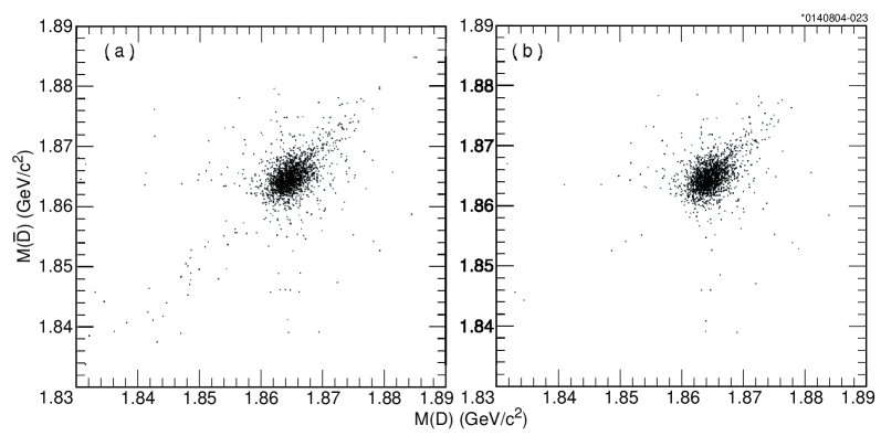
Figure 3: Scatter plot of $M(\bar{D})$ vs. $M(D)$ values for $\bar{D}^{0}\to K^{+}\pi^{-}\pi^{0}$ vs. $D^{0}\to K^{-}\pi^{+}\pi^{0}$ DT candidates from simulated events. (a) illustrates all candidates after imposing the $\Delta E$ requirement for each candidate given in Table 1. (b) illustrates the candidates remaining after choosing the candidate with the average $\widehat{M}(D)$ closest to $M_{D^{0}}$ in events with multiple candidates.

The components that must be included in the DT fits are illustrated in Fig. 3, which shows distributions of $M(\bar{D})$ vs. $M(D)$ for DT event candidates that are reconstructed in the $\bar{D}^{0}\to K^{+}\pi^{-}\pi^{0}$ and $D^{0}\to K^{-}\pi^{+}\pi^{0}$ modes. Figure 3(a) shows all candidates (including multiple candidates) after imposition of the $\Delta E$ requirement described in Sec. IV. The principal features of this two-dimensional distribution are:

• There is an obvious strong signal concentration with a complicated shape in the region surrounding $M(\bar{D})=M(D)=M_{D^{0}}$.

• There is a radiative tail above the signal peak at $45^{\circ}$ to the axes. This correlation is due to the fact that – neglecting measurement and reconstruction errors – the values of $M(D)$ and $M(\bar{D})$ calculated using the beam energy will both to be too large by the same amount if energy was lost due to ISR.

• There are faint horizontal and vertical bands at $M(\bar{D})=M_{D^{0}}$ and $M(D)=M_{D^{0}}$, respectively. The events in these bands are events in which the $\bar{D}^{0}$ ($D^{0}$) candidate was reconstructed correctly, but the $D^{0}$ ($\bar{D}^{0}$) was misreconstructed.

• There is a somewhat more visible band below the peak at $45^{\circ}$ to the axes that continues through the signal region and the radiative tail. This band is populated by two sources of background:

  • There are $D\bar{D}$ events, in which all of the particles were found and reconstructed reasonably accurately, but one or more particles from the real $D^{0}$ were interchanged with the corresponding particles from the $\bar{D}^{0}$, e.g., the two $\pi^{0}$s were interchanged.

  • There are also continuum events, i.e., annihilations into $u\bar{u}$, $d\bar{d}$, and $s\bar{s}$ quark pairs.

As illustrated in Fig. 3(b), all three bands below the peak are depopulated noticeably after choosing the candidate with the average mass $\widehat{M}(D)$ nearest to $M_{D^{0}}$. Since careful studies of this choice using Monte Carlo simulations of generic $D\bar{D}$ decays and continuum events showed no evidence of false peaks in the region of the $D$ mass, the net effect of this procedure is reduction of background without introduction of a false signal.

We included five terms in unbinned likelihood fits to account for these features of the two-dimensional $M(\bar{D})$ vs. $M(D)$ distributions. These terms were functions of $m=M(D)$, $\bar{m}=M(\bar{D})$, $\hat{m}=\widehat{M}(D)=[M(D)+M(\bar{D})]/2$, and $\delta m=[M(D)-M(\bar{D})]/2$. The terms are:

• $c(\hat{m};\mu,\sigma,\alpha,n)\,g(\delta m;\mu,\sigma_{\delta})$, a Crystal Ball function of $\hat{m}$ multiplied by a Gaussian function of $\delta m$. The Crystal Ball function models nearly all of the signal, including the radiative tail, while the Gaussian function models the effect of measurement errors in the direction transverse to $\hat{m}$. In these fits, $\mu$, $\sigma$, and $\sigma_{\delta}$ were allowed to float. The parameters $\mu$ and $\sigma$ also appear in other terms; they float in all terms, but their values are constrained to be identical in all terms. The parameters $\alpha$ and $n$ used in DT fits to data or Monte Carlo events with ISR, were fixed to the averages over all modes of the parameters obtained in ST fits to data or Monte Carlo events with ISR, respectively. In fits to Monte Carlo events without ISR the Crystal Ball function is replaced with a pure Gaussian. The values of Gaussian and Crystal Ball parameters obtained in DT yields are close to – but not exactly equal to – those obtained in the ST fits.

• $b(m;\mu,\rho_{L}\sigma,\rho_{R}\sigma)\,b(\bar{m};\mu,\rho_{L}\sigma,\rho_{R}\sigma)$, the product of two bifurcated Gaussian functions. These functions account for misreconstructed signal events as they did individually in ST fits. The ratios $\rho_{L}$ and $\rho_{R}$ were obtained from the fits to ST Monte Carlo events without ISR. The signal contribution is the sum of this contribution and the Crystal Ball contribution.

• $a(\hat{m};E_{0},\xi)\,g(\delta m;\mu,\sigma_{c})$, the product of an ARGUS background function of $\hat{m}$ and a Gaussian function of $\delta m$. This term models continuum background and any residual mispartitioned events remaining after choosing the value $\widehat{M}(D)$ closest to $M(D)$ in events with multiple candidates. The Gaussian parameter $\sigma_{c}$ is determined from continuum Monte Carlo events, and $\xi$ is allowed to float in the fit.

• $a(m;E_{0},\xi_{m})\,g(\bar{m};\mu,\sigma_{b})$, the product of an ARGUS function of $m$ and a Gaussian function of $\bar{m}$. This term models the horizontal band in the scatter plot. The values of $\xi_{m}$ and $\sigma_{b}$ are the identical in this term and the next. The value of $\sigma_{b}$ is determined from DT Monte Carlo events without ISR and is the same for all modes, while $\xi_{m}$ is allowed to float in the fits.

• $a(\bar{m};E_{0},\xi_{m})\,g(m;\mu,\sigma_{b})$, the product of an ARGUS function of $m$ and a Gaussian function of $\bar{m}$. This term models the vertical band in the scatter plot. The value of $\xi_{m}$ in this term is constrained to be equal to the value of $\xi_{m}$ in the term for the horizontal band.

Table 3: Double tag data yields and efficiencies and their statistical uncertainties.

$D$ Mode	$\bar{D}$ Mode	Yield ($10^{2}$)	Efficiency (%)
$D^{0}\to K^{-}\pi^{+}$	$\bar{D}^{0}\to K^{+}\pi^{-}$	$1.09\pm 0.11$	$42.6\pm 0.5$
$D^{0}\to K^{-}\pi^{+}\pi^{0}$	$\bar{D}^{0}\to K^{+}\pi^{-}\pi^{0}$	$4.84\pm 0.23$	$12.1\pm 0.3$
$D^{0}\to K^{-}\pi^{+}\pi^{+}\pi^{-}$	$\bar{D}^{0}\to K^{+}\pi^{-}\pi^{-}\pi^{+}$	$2.80\pm 0.17$	$20.8\pm 0.4$
$D^{0}\to K^{-}\pi^{+}$	$\bar{D}^{0}\to K^{+}\pi^{-}\pi^{0}$	$2.45\pm 0.16$	$23.2\pm 0.4$
$D^{0}\to K^{-}\pi^{+}\pi^{0}$	$\bar{D}^{0}\to K^{+}\pi^{-}$	$2.62\pm 0.16$	$22.6\pm 0.4$
$D^{0}\to K^{-}\pi^{+}$	$\bar{D}^{0}\to K^{+}\pi^{-}\pi^{-}\pi^{+}$	$2.05\pm 0.14$	$29.6\pm 0.4$
$D^{0}\to K^{-}\pi^{+}\pi^{+}\pi^{-}$	$\bar{D}^{0}\to K^{+}\pi^{-}$	$1.97\pm 0.14$	$29.6\pm 0.4$
$D^{0}\to K^{-}\pi^{+}\pi^{0}$	$\bar{D}^{0}\to K^{+}\pi^{-}\pi^{-}\pi^{+}$	$3.59\pm 0.20$	$15.2\pm 0.3$
$D^{0}\to K^{-}\pi^{+}\pi^{+}\pi^{-}$	$\bar{D}^{0}\to K^{+}\pi^{-}\pi^{0}$	$3.40\pm 0.19$	$15.5\pm 0.3$
$D^{+}\to K^{-}\pi^{+}\pi^{+}$	$D^{-}\to K^{+}\pi^{-}\pi^{-}$	$3.79\pm 0.20$	$26.7\pm 0.4$
$D^{+}\to K^{0}_{S}\pi^{+}$	$D^{-}\to K^{0}_{S}\pi^{-}$	$0.090\pm 0.030$	$20.6\pm 0.4$
$D^{+}\to K^{-}\pi^{+}\pi^{+}$	$D^{-}\to K^{0}_{S}\pi^{-}$	$0.609\pm 0.079$	$23.7\pm 0.4$
$D^{+}\to K^{0}_{S}\pi^{+}$	$D^{-}\to K^{+}\pi^{-}\pi^{-}$	$0.530\pm 0.073$	$23.9\pm 0.4$

Figures 4 and 5 show the projection of each of the “diagonal” $M(\bar{D})$ vs. $M(D)$ distributions projected onto the $M(D)$ axes. The fit in each figure is the sum of all terms in the fit projected on the $M(D)$ axis. Table 3 gives the DT yields in data and the corresponding DT efficiencies calculated from the signal Monte Carlo events with ISR. These quantities are used in the fit – described in Sec. X for branching fractions and numbers of $D\bar{D}$ events.

VIII Efficiencies in Data and Monte Carlo Events

We estimated efficiencies for reconstructing $D$ decays using Monte Carlo simulations. For precision measurements, we must also understand the accuracy with which the Monte Carlo events simulate tracking efficiencies. Using partial reconstruction techniques, we measure tracking efficiencies – in both data and Monte Carlo events – for charged pions and kaons, as well as the efficiency for detecting $K^{0}_{S}$ and $\pi^{0}$ mesons. For example, we fully reconstruct one $D^{0}$ and then combine it with one or more of the other particles in the event to partially reconstruct the $\bar{D}^{0}$, leaving out one particle – $\pi^{\pm}$, $K^{\pm}$, or $K^{0}_{S}$ – for which we wish to measure the efficiency. We calculate the square of the missing mass ($MM^{2}$) of the combination, which should peak at the mass squared of the missing particle. We then check whether the missing particle is actually detected or not, and we plot the missing mass squared for both classes of events. Fitting the signal peaks tells us what fraction of particles were actually detected. We also use similar techniques with $\psi^{\prime}\to J/\psi\,\pi^{+}\pi^{-}$ and $\psi^{\prime}\to J/\psi\,\pi^{0}\pi^{0}$ events to measure $\pi^{\pm}$ tracking efficiency at lower momenta and $\pi^{0}$ efficiency, respectively.

We illustrate this technique for measuring $K^{\pm}$ tracking efficiencies in Fig. 6, where – for both data and Monte Carlo events – we reconstruct $D^{0}$ mesons in the modes, $D^{0}\to K^{-}\pi^{+}$, $D^{0}\to K^{-}\pi^{+}\pi^{0}$, and $D^{0}\to K^{-}\pi^{+}\pi^{+}\pi^{-}$. We use the requirements $|M(D^{0})-M_{D^{0}}|<5$ MeV/$c^{2}$ and $|\Delta E|<25$ MeV to obtain a clean sample of $D^{0}$ decays. Figures 6(a) and 6(b) show the $MM^{2}$ distributions for data and Monte Carlo events, respectively, when the $K^{\pm}$ was found, while Figs. 6(c) and 6(d) show the corresponding $MM^{2}$ distributions for events in which the $K^{\pm}$ was not found. When the $K^{\pm}$ is found, there is a clean peak with little background in both data and Monte Carlo events. Each of these distributions is fit with two Gaussians of the same mean but different widths, and a small constant background. The widths of the Gaussians are somewhat different in data and Monte Carlo events. The $MM^{2}$ distributions for events in which the $K^{\pm}$ was not found are more complex. There is a peak at $M_{\pi^{+}}^{2}$ due to $D^{0}\to\pi^{+}\pi^{-}$ decays, and a peak at $M_{K^{+}}^{2}$ due to $\bar{D}^{0}\to K^{+}\pi^{-}$ decays. The shoulder on the right of each figure is due to $\bar{D}^{0}\to K^{+}\pi^{-}\pi^{0}$ decays in which only the $\pi^{-}$ is detected; its shape is well approximated by an error function. Finally, there is a linearly rising shape which describes the remaining backgrounds. We determine the parameters for the shapes of these backgrounds in fits to signal Monte Carlo events for these processes. We fit the data in Figs. 6(c) and 6(d) using these background shape parameters and the widths of the Gaussian parameters determined in fits to events in which the $K^{\pm}$ was detected.

For $\pi^{\pm}$ and $K^{\pm}$, we find evidence for slightly higher tracking efficiencies in data than in Monte Carlo events. Based on these preliminary studies, we increase the efficiencies determined from the Monte Carlo simulations by a factor of $1.03\pm 0.03$ for each charged track candidate used in the event. In our preliminary studies of $\pi^{0}$ efficiencies, we see no evidence for an efficiency difference between data and Monte Carlo events. Also, we find no evidence for a correction for $K^{0}_{S}$ decays beyond the factor of $1.03^{2}$ for the two charged daughter pions in the decay.

IX Systematic Errors

Table 4: Systematic uncertainties and the quantities to which they are applied in the branching fraction fit. Uncorrelated, additive uncertainties are given in the first section, and correlated, multiplicative uncertainties in the second.

Source	Fractional Uncertainty (%)	Quantity
Data processing	0.3	All yields
Yield fit functions	0.1–2.9	All yields
Background bias	2.5	DT yields
Double DCSD interference	0.8	Neutral DT yields
Detector simulation	3.0	Tracking efficiencies
	3.0	$K^{0}_{S}$ efficiencies
	4.4	$\pi^{0}$ efficiencies
	0.3	$\pi^{\pm}$ PID efficiencies
	1.0	$K^{\pm}$ PID efficiencies
Trigger simulation	0.3	ST efficiencies
Final state radiation	0.5	$D$ efficiencies
$|\Delta E|$ requirement	1.0	$D$ efficiencies, correlated by decay
Resonant substructure	3.0	$D^{0}\to K^{-}\pi^{+}\pi^{+}\pi^{-}$ efficiencies

We take systematic uncertainties into account directly in the branching fraction fit. Table 4 lists the uncertainties that we included and a brief description of each contribution follows.

• Data processing
  Potential losses of events in data processing has been limited to 0.3% and is assessed by reanalyzing the data with slightly different software configurations.

• Yield fit functions
  We gauge the sensitivity of the ST and DT yields to variations in the $M(D)$ fit functions by repeating the fits with different values of $\rho_{A}$, $\rho_{R}$, and $\rho_{L}$ as well as with different functional forms (such as a symmetric Gaussian instead of a bifurcated Gaussian for the wide signal component) and comparing efficiency-corrected yields.

• Background bias
  We estimate possible biases in the background parametrization from the agreement of the fit functions with the data. We find the discrepancies to be negligible for ST yields and as large as 2.5% for DT yields. Additional bias in the DT yields could have been introduced by the procedure for selecting the best candidate per event in double tags. However, as described in Sec. VII, we searched for this type of background in simulated continuum and generic $D\bar{D}$ Monte Carlo events and found no evidence of such a contamination.

• Double DCSD interference
  In the neutral DT modes, the Cabibbo-allowed amplitudes can interfere with amplitudes where both $D^{0}$ and $\bar{D}^{0}$ undergo doubly Cabibbo-suppressed decays (DCSD). We include an uncertainty to account for the unknown phase of this interference.

• Detector simulation – tracking, $K^{0}_{S}$, and $\pi^{0}$ efficiencies
  We estimate uncertainties due to differences between efficiencies in data and those estimated in Monte Carlo simulations using the partial reconstruction technique described in the previous section.

• Detector simulation – particle identification (PID) efficiencies
  Particle identification efficiencies are studied by reconstructing decays with unambiguous particle content, such as $D^{0}\to K^{0}_{S}\pi^{+}\pi^{-}$ and $\phi\to K^{+}K^{-}$. We also use $D^{0}\to K^{-}\pi^{+}\pi^{0}$, where the $K^{-}$ and $\pi^{+}$ are distinguished kinematically. The efficiencies in data are well-simulated by the Monte Carlo, and we assign correlated uncertainties of 0.3% and 1.0% to each $\pi^{+}$ and $K^{+}$, respectively. We do not assign these uncertainties to $K^{0}_{S}$ daughters, because they are not subjected to the $\pi^{+}$ identification requirements.

• Trigger simulation
  We assign a conservative uncertainty in the trigger simulation efficiency taken from the trigger inefficiency we find in simulations of the $D^{0}\to K^{-}\pi^{+}\pi^{0}$ mode.

• Final state radiation
  In Monte Carlo simulations, final state radiation typically reduces DT efficiencies by a factor of approximately two times the reduction of ST efficiencies. This leads to branching fraction values larger by 0.5% to 2% than they would be without including FSR in the Monte Carlo simulations. We have verified the accuracy of the FSR simulation to roughly 10% of itself using $\psi(2S)\to J/\psi\pi\pi$ decays, where $J/\psi\to\mu^{+}\mu^{-}\gamma$. For these preliminary results, we assign conservative uncertainties of 0.5% to ST efficiencies and 1.0% to DT efficiencies, correlated across all modes. This results in a $\pm 0.5$% correlated systematic error in branching fractions.

• $|\Delta E|$ requirement
  Discrepancies in detector resolution between data and Monte Carlo simulations can result in differences between the efficiencies of the $\Delta E$ requirement in data and Monte Carlo events. No evidence for such discrepancies has been found, and we include a systematic uncertainty of 1.0% for ST modes and 2.0% for DT modes, correlated by decay process.

• Resonant substructure
  The resonant substructure of $D^{0}\to K^{-}\pi^{+}\pi^{+}\pi^{-}$ in data is found to disagree with that in Monte Carlo simulations, introducing a possible fractional bias in efficiency of 3.0%. We apply a correlated systematic uncertainty of this size to all ST and DT modes with a $D^{0}\to K^{-}\pi^{+}\pi^{+}\pi^{-}$ decay.

For the $e^{+}e^{-}\to D\bar{D}$ cross section measurements, we include additional uncertainties from the luminosity measurement (3.0%) and from variations in the center-of-mass energy. We estimate the latter uncertainty by calculating $N_{D^{0}\bar{D}^{0}}$ and $N_{D^{+}D^{-}}$ in data taken at different values of $E_{\mathrm{cm}}$ in a 4 MeV region on the $\psi(3770)$. We find fractional variations of 2.5% in $N_{D^{0}\bar{D}^{0}}$ and 1.4% in $N_{D^{+}D^{-}}$, and include these numbers as systematic uncertainties.

Finally, we note that – although there are many contributions to the systematic errors listed in Table 4 – the contribution of tracking efficiencies dominates in this preliminary result. This is due to our conservative assignment of an error of $\pm 0.03n$, where $n$ is the number of tracks in a ST or DT mode for this uncertainty.

X Results of the Branching Fraction Fits

To determine the branching fractions ${\cal B}(D^{0}\to K^{-}\pi^{+})$, ${\cal B}(D^{0}\to K^{-}\pi^{+}\pi^{0})$, ${\cal B}(D^{0}\to K^{-}\pi^{+}\pi^{+}\pi^{-})$, ${\cal B}(D^{+}\to K^{-}\pi^{+}\pi^{+})$, and ${\cal B}(D^{+}\to K^{0}_{S}\pi^{+})$ as well as $N_{D^{0}\bar{D}^{0}}$ and $N_{D^{+}D^{-}}$, we measure event yields and efficiencies for the ten ST modes and thirteen DT modes, given in Tables 2 and 3. In the branching fraction fit, we correct these event yields not only for efficiency but also for crossfeed among the ST and DT modes and backgrounds from other $D$ decays. The estimated crossfeed and background contributions induce yield adjustments of 2% at most. Their dependence on the fit parameters is taken into account both in the yield subtraction and in the $\chi^{2}$ minimization. In addition to the correlated and uncorrelated systematic uncertainties, the statistical uncertainties on the yields, efficiencies, and background branching fractions are also included in the fit.

We validated the algorithm and the performance of the branching fit – as well as our entire analysis procedure – by measuring the branching fractions in generic Monte Carlo events. Since the generic Monte Carlo simulations were done without ISR, we used efficiencies obtained from signal Monte Carlo events without ISR. We find that the results of this procedure were in excellent agreement with the branching fractions used by EvtGen in generating the events. Furthermore, the generic Monte Carlo sample has an order of magnitude more events than our data, so the statistical errors in this test were about a factor of three smaller than the errors in the branching fractions obtained from data. The systematic errors were also substantially smaller than those estimated for data, so the agreement between measured and generated branching fractions of the generic Monte Carlo events is a very stringent test of our entire analysis procedure.

Table 5: Preliminary fitted branching fractions and $D\bar{D}$ pair yields. Uncertainties are statistical and systematic, respectively.

Parameter	Fitted Value	Fractional	Fractional
		Stat. Error	Syst. Error
$N_{D^{0}\bar{D}^{0}}$	$(1.98\pm 0.04\pm 0.03)\times 10^{5}$	1.9%	1.5%
${\cal B}(D^{0}\to K^{-}\pi^{+})$	$0.0392\pm 0.0008\pm 0.0023$	2.1%	5.8%
${\cal B}(D^{0}\to K^{-}\pi^{+}\pi^{0})$	$0.143\pm 0.003\pm 0.010$	2.0%	7.2%
${\cal B}(D^{0}\to K^{-}\pi^{+}\pi^{+}\pi^{-})$	$0.081\pm 0.002\pm 0.009$	2.1%	11.6%
$N_{D^{+}D^{-}}$	$(1.48\pm 0.06\pm 0.04)\times 10^{5}$	4.3%	2.4%
${\cal B}(D^{+}\to K^{-}\pi^{+}\pi^{+})$	$0.098\pm 0.004\pm 0.008$	4.4%	8.5%
${\cal B}(D^{+}\to K^{0}_{S}\pi^{+})$	$0.0161\pm 0.0008\pm 0.0015$	4.9%	9.1%
${{\cal B}(D^{0}\to K^{-}\pi^{+}\pi^{0})}/{{\cal B}(D^{0}\to K^{-}\pi^{+})}$	$3.64\pm 0.05\pm 0.17$	1.3%	4.8%
${{\cal B}(D^{0}\to K^{-}\pi^{+}\pi^{+}\pi^{-})}/{{\cal B}(D^{0}\to K^{-}\pi^{+})}$	$2.05\pm 0.03\pm 0.14$	1.4%	6.8%
${{\cal B}(D^{+}\to K^{0}_{S}\pi^{+})}/{{\cal B}(D^{+}\to K^{-}\pi^{+}\pi^{+})}$	$0.164\pm 0.004\pm 0.006$	2.5%	3.7%

The results of the data fit are shown in Table 5. The $\chi^{2}$ of the fit is 8.9 for 16 degrees of freedom, corresponding to a confidence level of 92%. To obtain the separate contributions from statistical and systematic uncertainties, we repeat the fit without any systematic inputs and take the quadrature difference of uncertainties. All five branching fractions are consistent with – but also higher than – the current PDG averages PDG . If no FSR is included in the simulations to calculate signal efficiencies, then all the branching fractions would be 0.5% to 2% lower. In addition, we compute ratios of branching fractions to the reference branching fractions, which have higher precision than the constituent branching fractions, and these also agree with the PDG averages. These ratios are also sensitive to final state radiation, and – without these corrections – all three ratios would be 1% to 2% higher.

Table 6: Correlation matrix, including systematic uncertainties, for the branching fractions determined from the fit.

	$N_{D^{0}\bar{D}^{0}}$	$K^{-}\pi^{+}$	$K^{-}\pi^{+}\pi^{0}$	$K^{-}\pi^{+}\pi^{-}\pi^{+}$	$N_{D^{+}D^{-}}$	$K^{-}\pi^{+}\pi^{+}$	$K^{0}_{S}\pi^{+}$
$N_{D^{0}\bar{D}^{0}}$	1	$-0.37$	$-0.26$	$-0.21$	$0.02$	$-0.02$	$-0.02$
$K^{-}\pi^{+}$		1	0.75	0.90	0.00	0.76	0.69
$K^{-}\pi^{+}\pi^{0}$			1	0.73	0.00	0.62	0.57
$K^{-}\pi^{+}\pi^{-}\pi^{+}$				1	0.00	0.80	0.73
$N_{D^{+}D^{-}}$					1	$-0.49$	$-0.47$
$K^{-}\pi^{+}\pi^{+}$						1	0.90
$K^{0}_{S}\pi^{+}$							1

The correlation matrix for the seven fit parameters is given in Table 6. In the absence of systematic uncertainties, there would be no correlation between the charged and neutral $D$ parameters. That these correlations are, in fact, large indicates that the precision of our branching fraction measurements is limited by our understanding of systematic effects.

We obtain the $e^{+}e^{-}\to D\bar{D}$ cross sections by dividing the fitted values of $N_{D^{0}\bar{D}^{0}}$ and $N_{D^{+}D^{-}}$ by the luminosity collected on the $\psi(3770)$, which we determine to be ${\cal L}=57.2\pm 1.7$  pb^-1. Thus, at $E_{\mathrm{cm}}=3773$ MeV, we find preliminary values of the production cross sections,

$$\sigma(e^{+}e^{-}\to D^{0}\bar{D}^{0}) = (3.47\pm 0.07\pm 0.15)\ {\rm nb}$$

$$\sigma(e^{+}e^{-}\to D^{+}D^{-}) = (2.59\pm 0.11\pm 0.11)\ {\rm nb}$$

$$\sigma(e^{+}e^{-}\to D\bar{D}) = (6.06\pm 0.13\pm 0.22)\ {\rm nb}$$

$$\sigma(e^{+}e^{-}\to D^{+}D^{-})/\sigma(e^{+}e^{-}\to D^{0}\bar{D}^{0}) = \hskip 3.99994pt0.75\pm 0.04\pm 0.02,$$

where the uncertainties are statistical and systematic, respectively. The charged and neutral cross sections have a correlation coefficient of 0.32 stemming from the common use of the luminosity measurement.

XI Conclusions

We report preliminary measurements of three $D^{0}$ and two $D^{+}$ branching fractions in a sample of nearly 60 pb^-1 of $e^{+}e^{-}\to D\bar{D}$ data obtained at $E_{\mathrm{cm}}=3.77$ GeV. The results are presented in Table 5 and the correlation coefficients among the results are given in Table 6. We find branching fractions in agreement with – but somewhat higher – than those in the PDG PDG summary. We note that the Monte Carlo simulations used in calculating efficiencies in this analysis included final state radiation. However, the branching fractions used in the Particle Data Group averages do not include this effect. If we had not included final state radiation in our simulations, branching fractions would have been 0.5% to 2% lower. At this preliminary stage in our analysis, the systematic errors are factors of approximately 2 to 5 larger than the statistical errors. Our statistical errors for branching fractions and ratios of branching fractions are – in nearly all cases – less than the statistical errors in the individual measurements that contributed to the PDG averages.

Our techniques for event selection, for fitting data and Monte Carlo distributions to obtain yields and efficiencies, and for fitting the results to obtain branching fractions are validated with generic Monte Carlo events to a much higher precision than the statistical errors from the current data sample. This indicates that we can improve the results from these data substantially with more detailed understanding of any possible systematic differences between our data and our Monte Carlo simulations. Our systematic errors are dominated by the uncertainty of $0.03n$, where $n$ is the number of charged tracks in a ST or DT mode, that we assign for the difference between tracking efficiency in data and Monte Carlo simulations. Many of the systematic uncertainties, such as those for tracking and particle identification efficiencies, will be improved with larger data samples.

Our preliminary measurements of the production cross sections $\sigma(D^{0}\bar{D}^{0})$, $\sigma(D^{+}D^{-})$, and $\sigma(D\bar{D})$ are in good agreement with the cross sections measured by the MARK III collaboration markiii-2 and in excellent agreement with recent BES results reported at the 2004 Moriond conference bes-sigmaddbar .

XII Acknowledgements

We gratefully acknowledge the effort of the CESR staff in providing us with excellent luminosity and running conditions. This work was supported by the National Science Foundation, the U.S. Department of Energy, the Research Corporation, and the Texas Advanced Research Program.

Figure 1: Distributions of calculated $M(D)$ values for single tag neutral $D$ candidates in data with $D^{0}$ and $\bar{D}^{0}$ combined in each mode. The points are data and the curves are fits to the data. In each plot, the dotted curve shows the contribution of the ARGUS background function, the dashed curve shows the contribution of the bifurcated Gaussian, and the solid curve shows the total, including the Crystal Ball function. (a) and (b) illustrate $D^{0}\to K^{-}\pi^{+}$ candidates, (c) and (d) illustrate $D^{0}\to K^{-}\pi^{+}\pi^{0}$ candidates, and (e) and (f) illustrate $D^{0}\to K^{-}\pi^{+}\pi^{+}\pi^{-}$ candidates.

Figure 2: Distributions of calculated $M(D)$ values for single tag charged $D$ candidates in data with $D^{+}$ and $D^{-}$ combined in each mode. The points are data and the curves are fits to the data. In each plot, the dotted curve shows the contribution of the ARGUS background function, the dashed curve shows the contribution of the bifurcated Gaussian, and the solid curve shows the total, including the Crystal Ball function. (a) and (b) illustrate $D^{+}\to K^{-}\pi^{+}\pi^{+}$ candidates and (c) and (d) illustrate $D^{+}\to K^{0}_{S}\pi^{+}$ candidates.

Figure 4: Projections of double tag $D^{0}$-$\bar{D}^{0}$ candidate masses on the $M(D)$ axis, with the $D^{0}$ and $\bar{D}^{0}$ reconstructed in corresponding charge conjugate modes. Projections of the candidate masses on the $M(\bar{D})$ axis are nearly identical. (a) illustrates $D^{0}\to K^{-}\pi^{+}$ candidates, (b) illustrates $D^{0}\to K^{-}\pi^{+}\pi^{0}$ candidates, and (c) illustrates $D^{0}\to K^{-}\pi^{+}\pi^{+}\pi^{-}$ candidates.

Figure 5: Projections of double tag $D^{+}$-$D^{-}$ candidate masses on the $M(D)$ axis, with the $D^{+}$ and $D^{-}$ reconstructed in corresponding charge conjugate modes. Projections of the candidate masses on the $M(\bar{D})$ axis are nearly identical. (a) illustrates $D^{+}\to K^{-}\pi^{+}\pi^{+}$ candidates and (b) illustrates $D^{+}\to K^{0}_{S}\pi^{+}$ candidates.

Figure 6: Missing mass squared distributions for measuring $K^{\pm}$ efficiencies in data and Monte Carlo events in which a $D^{0}$ has been found. (a) and (b) data and Monte Carlo events, respectively, in which the $K^{+}$ from $\bar{D}^{0}\to K^{+}\pi^{-}$ decay was found. (c) and (d) data and Monte Carlo events, respectively, in which the $K^{+}$ from $\bar{D}^{0}\to K^{+}\pi^{-}$ decay was not found.

References

- (1) Particle Data Group, S. Eidelman et al., Phys. Lett. B 592, 1 (2004).
- (2) MARK III Collaboration, R.M. Baltrusaitis et al., Phys. Rev. Lett. 56, 2140 (1986).
- (3) MARK III Collaboration, J. Adler et al., Phys. Rev. Lett. 60, 89 (1988).
- (4) W. Sun (to be published).
- (5) CLEO Collaboration, Y. Kubota et al., Nucl. Instrum. Methods Phys. Res., Sec. A 320, 66 (1992).
- (6) D. Peterson et al., Nucl. Instrum. Methods Phys. Res., Sec. A 478, 142 (2002).
- (7) M. Artuso et al., Nucl. Instrum. Methods Phys. Res., Sec. A 502, 91 (2003).
- (8) CLEO-c/CESR-c Taskforces & CLEO-c Collaboration, Cornell LEPP preprint CLNS 01/1742 (2001).
- (9) CLEO Collaboration, G. Crawford et al., Nucl. Instrum. Methods Phys. Res., Sec. A 345, 429 (1992).
- (10) C.M. Carloni Calame et al., in Proceedings of the Workshop on Hadronic Cross Section at Low Energy (SIGHAD03), Pisa, Italy, 2003 (to be published) (hep-ph/0312014).
- (11) R. Brun et al., GEANT 3.21, CERN Program Library Long Writeup W5013 (unpublished) 1993.
- (12) D.J. Lange, Nucl. Instrum. Methods Phys. Res., Sec. A 462, 152 (2001).
- (13) E. Barberio and Z. Was, Comput. Phys. Commun. 79, 291 (1994).
- (14) Particle Data Group, K. Hagiwara et al., Phys. Rev. D 66, 010001 (2002).
- (15) ARGUS Collaboration, H. Albrecht et al., Phys. Lett. B 241, 278 (1990).
- (16) Tomasz Skwarnicki, Ph.D. thesis, Institute of Nuclear Physics, Cracow, 1986, DESY Report No. DESY F31-86-02.
- (17) R. Gong for the BES Collaboration, in Proceedings of the 39th Reconcontres de Moriond o Electroweak Interactions and Unified Theories, La Thuile, Aoasta Valley, Italy, 21-28 March, 2004 (to be published) (hep-ex/0406027).