BABAR-CONF-04/14
SLAC-PUB-10601
July 2004
Amplitude Analysis of and
The BABAR Collaboration
Abstract
We present preliminary results of a maximum-likelihood Dalitz-plot analysis of the charmless hadronic decays to the final states and from data corresponding to an integrated on-resonance luminosity of 166 recorded by the BABAR experiment at the SLAC PEP-II asymmetric-energy Factory. We measure the total branching fractions and , and provide fit fractions and phases for intermediate resonance states.
Submitted to the 32nd International Conference on High-Energy Physics, ICHEP 04,
16 August—22 August 2004, Beijing, China
Stanford Linear Accelerator Center, Stanford University, Stanford, CA 94309
Work supported in part by Department of Energy contract DE-AC03-76SF00515.
The BABAR Collaboration,
B. Aubert, R. Barate, D. Boutigny, F. Couderc, J.-M. Gaillard, A. Hicheur, Y. Karyotakis, J. P. Lees, V. Tisserand, A. Zghiche
Laboratoire de Physique des Particules, F-74941 Annecy-le-Vieux, France
A. Palano, A. Pompili
Università di Bari, Dipartimento di Fisica and INFN, I-70126 Bari, Italy
J. C. Chen, N. D. Qi, G. Rong, P. Wang, Y. S. Zhu
Institute of High Energy Physics, Beijing 100039, China
G. Eigen, I. Ofte, B. Stugu
University of Bergen, Inst. of Physics, N-5007 Bergen, Norway
G. S. Abrams, A. W. Borgland, A. B. Breon, D. N. Brown, J. Button-Shafer, R. N. Cahn, E. Charles, C. T. Day, M. S. Gill, A. V. Gritsan, Y. Groysman, R. G. Jacobsen, R. W. Kadel, J. Kadyk, L. T. Kerth, Yu. G. Kolomensky, G. Kukartsev, G. Lynch, L. M. Mir, P. J. Oddone, T. J. Orimoto, M. Pripstein, N. A. Roe, M. T. Ronan, V. G. Shelkov, W. A. Wenzel
Lawrence Berkeley National Laboratory and University of California, Berkeley, CA 94720, USA
M. Barrett, K. E. Ford, T. J. Harrison, A. J. Hart, C. M. Hawkes, S. E. Morgan, A. T. Watson
University of Birmingham, Birmingham, B15 2TT, United Kingdom
M. Fritsch, K. Goetzen, T. Held, H. Koch, B. Lewandowski, M. Pelizaeus, M. Steinke
Ruhr Universität Bochum, Institut für Experimentalphysik 1, D-44780 Bochum, Germany
J. T. Boyd, N. Chevalier, W. N. Cottingham, M. P. Kelly, T. E. Latham, F. F. Wilson
University of Bristol, Bristol BS8 1TL, United Kingdom
T. Cuhadar-Donszelmann, C. Hearty, N. S. Knecht, T. S. Mattison, J. A. McKenna, D. Thiessen
University of British Columbia, Vancouver, BC, Canada V6T 1Z1
A. Khan, P. Kyberd, L. Teodorescu
Brunel University, Uxbridge, Middlesex UB8 3PH, United Kingdom
A. E. Blinov, V. E. Blinov, V. P. Druzhinin, V. B. Golubev, V. N. Ivanchenko, E. A. Kravchenko, A. P. Onuchin, S. I. Serednyakov, Yu. I. Skovpen, E. P. Solodov, A. N. Yushkov
Budker Institute of Nuclear Physics, Novosibirsk 630090, Russia
D. Best, M. Bruinsma, M. Chao, I. Eschrich, D. Kirkby, A. J. Lankford, M. Mandelkern, R. K. Mommsen, W. Roethel, D. P. Stoker
University of California at Irvine, Irvine, CA 92697, USA
C. Buchanan, B. L. Hartfiel
University of California at Los Angeles, Los Angeles, CA 90024, USA
S. D. Foulkes, J. W. Gary, B. C. Shen, K. Wang
University of California at Riverside, Riverside, CA 92521, USA
D. del Re, H. K. Hadavand, E. J. Hill, D. B. MacFarlane, H. P. Paar, Sh. Rahatlou, V. Sharma
University of California at San Diego, La Jolla, CA 92093, USA
J. W. Berryhill, C. Campagnari, B. Dahmes, O. Long, A. Lu, M. A. Mazur, J. D. Richman, W. Verkerke
University of California at Santa Barbara, Santa Barbara, CA 93106, USA
T. W. Beck, A. M. Eisner, C. A. Heusch, J. Kroseberg, W. S. Lockman, G. Nesom, T. Schalk, B. A. Schumm, A. Seiden, P. Spradlin, D. C. Williams, M. G. Wilson
University of California at Santa Cruz, Institute for Particle Physics, Santa Cruz, CA 95064, USA
J. Albert, E. Chen, G. P. Dubois-Felsmann, A. Dvoretskii, D. G. Hitlin, I. Narsky, T. Piatenko, F. C. Porter, A. Ryd, A. Samuel, S. Yang
California Institute of Technology, Pasadena, CA 91125, USA
S. Jayatilleke, G. Mancinelli, B. T. Meadows, M. D. Sokoloff
University of Cincinnati, Cincinnati, OH 45221, USA
T. Abe, F. Blanc, P. Bloom, S. Chen, W. T. Ford, U. Nauenberg, A. Olivas, P. Rankin, J. G. Smith, J. Zhang, L. Zhang
University of Colorado, Boulder, CO 80309, USA
A. Chen, J. L. Harton, A. Soffer, W. H. Toki, R. J. Wilson, Q. Zeng
Colorado State University, Fort Collins, CO 80523, USA
D. Altenburg, T. Brandt, J. Brose, M. Dickopp, E. Feltresi, A. Hauke, H. M. Lacker, R. Müller-Pfefferkorn, R. Nogowski, S. Otto, A. Petzold, J. Schubert, K. R. Schubert, R. Schwierz, B. Spaan, J. E. Sundermann
Technische Universität Dresden, Institut für Kern- und Teilchenphysik, D-01062 Dresden, Germany
D. Bernard, G. R. Bonneaud, F. Brochard, P. Grenier, S. Schrenk, Ch. Thiebaux, G. Vasileiadis, M. Verderi
Ecole Polytechnique, LLR, F-91128 Palaiseau, France
D. J. Bard, P. J. Clark, D. Lavin, F. Muheim, S. Playfer, Y. Xie
University of Edinburgh, Edinburgh EH9 3JZ, United Kingdom
M. Andreotti, V. Azzolini, D. Bettoni, C. Bozzi, R. Calabrese, G. Cibinetto, E. Luppi, M. Negrini, L. Piemontese, A. Sarti
Università di Ferrara, Dipartimento di Fisica and INFN, I-44100 Ferrara, Italy
E. Treadwell
Florida A&M University, Tallahassee, FL 32307, USA
F. Anulli, R. Baldini-Ferroli, A. Calcaterra, R. de Sangro, G. Finocchiaro, P. Patteri, I. M. Peruzzi, M. Piccolo, A. Zallo
Laboratori Nazionali di Frascati dell’INFN, I-00044 Frascati, Italy
A. Buzzo, R. Capra, R. Contri, G. Crosetti, M. Lo Vetere, M. Macri, M. R. Monge, S. Passaggio, C. Patrignani, E. Robutti, A. Santroni, S. Tosi
Università di Genova, Dipartimento di Fisica and INFN, I-16146 Genova, Italy
S. Bailey, G. Brandenburg, K. S. Chaisanguanthum, M. Morii, E. Won
Harvard University, Cambridge, MA 02138, USA
R. S. Dubitzky, U. Langenegger
Universität Heidelberg, Physikalisches Institut, Philosophenweg 12, D-69120 Heidelberg, Germany
W. Bhimji, D. A. Bowerman, P. D. Dauncey, U. Egede, J. R. Gaillard, G. W. Morton, J. A. Nash, M. B. Nikolich, G. P. Taylor
Imperial College London, London, SW7 2AZ, United Kingdom
M. J. Charles, G. J. Grenier, U. Mallik
University of Iowa, Iowa City, IA 52242, USA
J. Cochran, H. B. Crawley, J. Lamsa, W. T. Meyer, S. Prell, E. I. Rosenberg, A. E. Rubin, J. Yi
Iowa State University, Ames, IA 50011-3160, USA
M. Biasini, R. Covarelli, M. Pioppi
Università di Perugia, Dipartimento di Fisica and INFN, I-06100 Perugia, Italy
M. Davier, X. Giroux, G. Grosdidier, A. Höcker, S. Laplace, F. Le Diberder, V. Lepeltier, A. M. Lutz, T. C. Petersen, S. Plaszczynski, M. H. Schune, L. Tantot, G. Wormser
Laboratoire de l’Accélérateur Linéaire, F-91898 Orsay, France
C. H. Cheng, D. J. Lange, M. C. Simani, D. M. Wright
Lawrence Livermore National Laboratory, Livermore, CA 94550, USA
A. J. Bevan, C. A. Chavez, J. P. Coleman, I. J. Forster, J. R. Fry, E. Gabathuler, R. Gamet, D. E. Hutchcroft, R. J. Parry, D. J. Payne, R. J. Sloane, C. Touramanis
University of Liverpool, Liverpool L69 72E, United Kingdom
J. J. Back,111Now at Department of Physics, University of Warwick, Coventry, United Kingdom C. M. Cormack, P. F. Harrison,11footnotemark: 1 F. Di Lodovico, G. B. Mohanty11footnotemark: 1
Queen Mary, University of London, E1 4NS, United Kingdom
C. L. Brown, G. Cowan, R. L. Flack, H. U. Flaecher, M. G. Green, P. S. Jackson, T. R. McMahon, S. Ricciardi, F. Salvatore, M. A. Winter
University of London, Royal Holloway and Bedford New College, Egham, Surrey TW20 0EX, United Kingdom
D. Brown, C. L. Davis
University of Louisville, Louisville, KY 40292, USA
J. Allison, N. R. Barlow, R. J. Barlow, P. A. Hart, M. C. Hodgkinson, G. D. Lafferty, A. J. Lyon, J. C. Williams
University of Manchester, Manchester M13 9PL, United Kingdom
A. Farbin, W. D. Hulsbergen, A. Jawahery, D. Kovalskyi, C. K. Lae, V. Lillard, D. A. Roberts
University of Maryland, College Park, MD 20742, USA
G. Blaylock, C. Dallapiccola, K. T. Flood, S. S. Hertzbach, R. Kofler, V. B. Koptchev, T. B. Moore, S. Saremi, H. Staengle, S. Willocq
University of Massachusetts, Amherst, MA 01003, USA
R. Cowan, G. Sciolla, S. J. Sekula, F. Taylor, R. K. Yamamoto
Massachusetts Institute of Technology, Laboratory for Nuclear Science, Cambridge, MA 02139, USA
D. J. J. Mangeol, P. M. Patel, S. H. Robertson
McGill University, Montréal, QC, Canada H3A 2T8
A. Lazzaro, V. Lombardo, F. Palombo
Università di Milano, Dipartimento di Fisica and INFN, I-20133 Milano, Italy
J. M. Bauer, L. Cremaldi, V. Eschenburg, R. Godang, R. Kroeger, J. Reidy, D. A. Sanders, D. J. Summers, H. W. Zhao
University of Mississippi, University, MS 38677, USA
S. Brunet, D. Côté, P. Taras
Université de Montréal, Laboratoire René J. A. Lévesque, Montréal, QC, Canada H3C 3J7
H. Nicholson
Mount Holyoke College, South Hadley, MA 01075, USA
N. Cavallo,222Also with Università della Basilicata, Potenza, Italy F. Fabozzi,22footnotemark: 2 C. Gatto, L. Lista, D. Monorchio, P. Paolucci, D. Piccolo, C. Sciacca
Università di Napoli Federico II, Dipartimento di Scienze Fisiche and INFN, I-80126, Napoli, Italy
M. Baak, H. Bulten, G. Raven, H. L. Snoek, L. Wilden
NIKHEF, National Institute for Nuclear Physics and High Energy Physics, NL-1009 DB Amsterdam, The Netherlands
C. P. Jessop, J. M. LoSecco
University of Notre Dame, Notre Dame, IN 46556, USA
T. Allmendinger, K. K. Gan, K. Honscheid, D. Hufnagel, H. Kagan, R. Kass, T. Pulliam, A. M. Rahimi, R. Ter-Antonyan, Q. K. Wong
Ohio State University, Columbus, OH 43210, USA
J. Brau, R. Frey, O. Igonkina, C. T. Potter, N. B. Sinev, D. Strom, E. Torrence
University of Oregon, Eugene, OR 97403, USA
F. Colecchia, A. Dorigo, F. Galeazzi, M. Margoni, M. Morandin, M. Posocco, M. Rotondo, F. Simonetto, R. Stroili, G. Tiozzo, C. Voci
Università di Padova, Dipartimento di Fisica and INFN, I-35131 Padova, Italy
M. Benayoun, H. Briand, J. Chauveau, P. David, Ch. de la Vaissière, L. Del Buono, O. Hamon, M. J. J. John, Ph. Leruste, J. Malcles, J. Ocariz, M. Pivk, L. Roos, S. T’Jampens, G. Therin
Universités Paris VI et VII, Laboratoire de Physique Nucléaire et de Hautes Energies, F-75252 Paris, France
P. F. Manfredi, V. Re
Università di Pavia, Dipartimento di Elettronica and INFN, I-27100 Pavia, Italy
P. K. Behera, L. Gladney, Q. H. Guo, J. Panetta
University of Pennsylvania, Philadelphia, PA 19104, USA
C. Angelini, G. Batignani, S. Bettarini, M. Bondioli, F. Bucci, G. Calderini, M. Carpinelli, F. Forti, M. A. Giorgi, A. Lusiani, G. Marchiori, F. Martinez-Vidal,333Also with IFIC, Instituto de Física Corpuscular, CSIC-Universidad de Valencia, Valencia, Spain M. Morganti, N. Neri, E. Paoloni, M. Rama, G. Rizzo, F. Sandrelli, J. Walsh
Università di Pisa, Dipartimento di Fisica, Scuola Normale Superiore and INFN, I-56127 Pisa, Italy
M. Haire, D. Judd, K. Paick, D. E. Wagoner
Prairie View A&M University, Prairie View, TX 77446, USA
N. Danielson, P. Elmer, Y. P. Lau, C. Lu, V. Miftakov, J. Olsen, A. J. S. Smith, A. V. Telnov
Princeton University, Princeton, NJ 08544, USA
F. Bellini, G. Cavoto,444Also with Princeton University, Princeton, USA R. Faccini, F. Ferrarotto, F. Ferroni, M. Gaspero, L. Li Gioi, M. A. Mazzoni, S. Morganti, M. Pierini, G. Piredda, F. Safai Tehrani, C. Voena
Università di Roma La Sapienza, Dipartimento di Fisica and INFN, I-00185 Roma, Italy
S. Christ, G. Wagner, R. Waldi
Universität Rostock, D-18051 Rostock, Germany
T. Adye, N. De Groot, B. Franek, N. I. Geddes, G. P. Gopal, E. O. Olaiya
Rutherford Appleton Laboratory, Chilton, Didcot, Oxon, OX11 0QX, United Kingdom
R. Aleksan, S. Emery, A. Gaidot, S. F. Ganzhur, P.-F. Giraud, G. Hamel de Monchenault, W. Kozanecki, M. Legendre, G. W. London, B. Mayer, G. Schott, G. Vasseur, Ch. Yèche, M. Zito
DSM/Dapnia, CEA/Saclay, F-91191 Gif-sur-Yvette, France
M. V. Purohit, A. W. Weidemann, J. R. Wilson, F. X. Yumiceva
University of South Carolina, Columbia, SC 29208, USA
D. Aston, R. Bartoldus, N. Berger, A. M. Boyarski, O. L. Buchmueller, R. Claus, M. R. Convery, M. Cristinziani, G. De Nardo, D. Dong, J. Dorfan, D. Dujmic, W. Dunwoodie, E. E. Elsen, S. Fan, R. C. Field, T. Glanzman, S. J. Gowdy, T. Hadig, V. Halyo, C. Hast, T. Hryn’ova, W. R. Innes, M. H. Kelsey, P. Kim, M. L. Kocian, D. W. G. S. Leith, J. Libby, S. Luitz, V. Luth, H. L. Lynch, H. Marsiske, R. Messner, D. R. Muller, C. P. O’Grady, V. E. Ozcan, A. Perazzo, M. Perl, S. Petrak, B. N. Ratcliff, A. Roodman, A. A. Salnikov, R. H. Schindler, J. Schwiening, G. Simi, A. Snyder, A. Soha, J. Stelzer, D. Su, M. K. Sullivan, J. Va’vra, S. R. Wagner, M. Weaver, A. J. R. Weinstein, W. J. Wisniewski, M. Wittgen, D. H. Wright, A. K. Yarritu, C. C. Young
Stanford Linear Accelerator Center, Stanford, CA 94309, USA
P. R. Burchat, A. J. Edwards, T. I. Meyer, B. A. Petersen, C. Roat
Stanford University, Stanford, CA 94305-4060, USA
S. Ahmed, M. S. Alam, J. A. Ernst, M. A. Saeed, M. Saleem, F. R. Wappler
State University of New York, Albany, NY 12222, USA
W. Bugg, M. Krishnamurthy, S. M. Spanier
University of Tennessee, Knoxville, TN 37996, USA
R. Eckmann, H. Kim, J. L. Ritchie, A. Satpathy, R. F. Schwitters
University of Texas at Austin, Austin, TX 78712, USA
J. M. Izen, I. Kitayama, X. C. Lou, S. Ye
University of Texas at Dallas, Richardson, TX 75083, USA
F. Bianchi, M. Bona, F. Gallo, D. Gamba
Università di Torino, Dipartimento di Fisica Sperimentale and INFN, I-10125 Torino, Italy
L. Bosisio, C. Cartaro, F. Cossutti, G. Della Ricca, S. Dittongo, S. Grancagnolo, L. Lanceri, P. Poropat,555Deceased L. Vitale, G. Vuagnin
Università di Trieste, Dipartimento di Fisica and INFN, I-34127 Trieste, Italy
R. S. Panvini
Vanderbilt University, Nashville, TN 37235, USA
Sw. Banerjee, C. M. Brown, D. Fortin, P. D. Jackson, R. Kowalewski, J. M. Roney, R. J. Sobie
University of Victoria, Victoria, BC, Canada V8W 3P6
H. R. Band, B. Cheng, S. Dasu, M. Datta, A. M. Eichenbaum, M. Graham, J. J. Hollar, J. R. Johnson, P. E. Kutter, H. Li, R. Liu, A. Mihalyi, A. K. Mohapatra, Y. Pan, R. Prepost, P. Tan, J. H. von Wimmersperg-Toeller, J. Wu, S. L. Wu, Z. Yu
University of Wisconsin, Madison, WI 53706, USA
M. G. Greene, H. Neal
Yale University, New Haven, CT 06511, USA
1 Introduction
The study of charmless hadronic decays can make important contributions to the understanding of CP violation in the Standard Model as well as to models of hadronic decays. The -meson decay to the three-body final state can proceed via intermediate resonances formed from two of the particles. These two-body states can interfere with each other and with the nonresonant three-body decay. The three-body state is unique in the search for weak phases as it is possible to determine the strong phase variation for overlapping resonances. Studies of these decays can also help to clarify the nature of the resonances involved, not all of which are well understood. A full Dalitz-plot analysis is necessary to correctly model this interference and extract branching fractions.
Observations of -meson decays to the and three-body final states have already been reported by the Belle and BABAR collaborations using a method that treats each intermediate decay incoherently [1, 2, 3]. Belle has also reported a preliminary Dalitz-plot analysis of the decay [4]. We present a preliminary Dalitz-plot analysis for both the and decay modes.
2 The BABAR Detector and Data Sample
Here we present preliminary results from a full amplitude analysis based on a 166 data sample containing 182 million pairs collected with the BABAR detector [5] at the SLAC PEP-II asymmetric-energy storage ring [6] operating at the resonance at a center-of-mass energy of . An additional total integrated luminosity of 16 was recorded at an energy below this energy and is used to study backgrounds from continuum production. The charm decay , is used as a calibration channel as it has a relatively high branching fraction.
Details of the BABAR detector are described elsewhere [5]. The specific components used for this paper are charged particle tracking provided by a combination of a silicon vertex tracker (SVT), which consists of five layers of double-sided detectors, and a 40-layer central drift chamber (DCH) in a 1.5-T solenoidal magnetic field. This allows a transverse momentum resolution for the combined tracking system of , where the sum is in quadrature and is measured in . Charged-particle identification is provided by combining information on the average energy loss in the two tracking devices and the angle of emission of Cherenkov radiation in an internally reflecting ring-imaging Cherenkov detector (DIRC) covering the central region. The resolution from the drift chamber is typically about for pions. The Cherenkov angle resolution of the DIRC is measured to be 2.4 mrad, which provides nearly separation between charged kaons and pions at a momentum of 3 .
3 Event Selection and Reconstruction
-meson candidates are reconstructed from events that have four or more charged tracks. Each track is required to have at least 12 hits in the DCH, a minimum transverse momentum of 100 , and a distance of closest approach to the primary vertex of less than 1.5 in the transverse plane and less than 10 along the beam axis. Charged tracks identified as leptons are rejected. The -meson candidates are formed from three-charged-track combinations and particle identification criteria are applied. The average selection efficiency for kaons in our final state that have passed the tracking requirements is including geometrical acceptance, while the misidentification probability of pions as kaons is below 5% at all momenta. The kaon veto on pions in our final state is efficient. The -meson candidates’ energies and momenta are required to satisfy appropriate kinematic constraints, as detailed in Section 5.
4 Background Suppression and Characterisation
The dominant source of background comes from light quark and charm continuum production. This background is suppressed by imposing requirements on event-shape variables calculated in the rest frame. The first discriminating variable is , the cosine of the angle between the thrust axis of the selected candidate and the thrust axis of the rest of the event. For continuum background the distribution of is strongly peaked towards unity whereas the distribution is uniform for signal events. We require for and for .111Charge-conjugate states are implied throughout this section.
Additionally, we make requirements on a Fisher discriminant [7] formed using a linear combination of nine variables representing the angular distribution of the energy flow of the rest of the event into each of nine two-sided concentric 10∘ cones around the thrust axis of the reconstructed [8].
Other backgrounds arise from events. There are four main sources: combinatorial background from three unrelated tracks; three- and four-body decays, where represents other particles in the final state; charmless four-body decays with a missing particle and three-body decays with one or more particles misidentified. In the case of charm decays with large branching fractions these backgrounds are greatly reduced by vetoing the appropriate region of the two-body invariant-mass spectra. The rejected decays and the invariant-mass veto ranges are given in Table 1.
| Resonance | ||
|---|---|---|
| (or ) |
The remaining charm backgrounds that escape the vetoes and backgrounds from charmless decays are studied using a large sample of Monte Carlo (MC) simulated decays equivalent to approximately five times the integrated luminosity for the data. Any events that pass the selection criteria are further studied using exclusive MC samples to estimate reconstruction efficiency and yields. The and Dalitz distributions of the backgrounds, which are used in the likelihood fits, are then normalised to the total number of predicted events in the final data sample. For , we expect -related background events, dominated by the decays and . For , we expect background events and the dominant backgrounds come from -meson decays to states containing a or and a or , the decays and , and the nonresonant decay .
A further background in this analysis comes from signal events that have been misreconstructed by switching one or more particles from the decay of the signal meson with particles from the other meson in the event. The amount of this background is estimated from MC studies, and for both and is found to be a very small effect that accounts for less than 2% of the final data sample in the signal box (defined in Section 5). As such it is neglected in the analysis.
Both the continuum and -related backgrounds are modeled in the Dalitz amplitude fit using linearly interpolated 2-dimensional histograms.
5 Final Data Selection
Two kinematic variables are used to select a final data sample. The first variable is , the difference between the center of mass (CM) energy of the -meson candidate and , where is the total CM energy. The second is the energy-substituted mass where pB is the momentum and (Ei,pi) is the four-momentum of the initial state. The mean of the distribution is shifted by as measured from the calibration channel . For we require ; for the requirement is where the lower edge is tightened by 30 to reduce specific backgrounds.
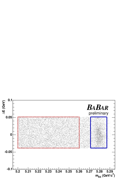
We define three regions in the - plane, illustrated in Figure 1. The signal box is defined by and events in this region are used in the amplitude analysis. The signal strip is defined by and is used to determine the fraction of signal and continuum events in the signal box. A sideband area below the signal box, defined by , is used to obtain the distribution of the continuum events in the Dalitz plane.
We accept one -meson candidate per event in the signal strip. Fewer than 3% of events have multiple candidates and in those events one candidate is randomly accepted to avoid bias.
After all selection criteria are applied the average efficiency for reconstruction of phase space and MC events in the signal box is % and %, respectively, where the errors are statistical only. The efficiency across the Dalitz plot is uniform except for very small decreases near the boundaries. In the amplitude analysis, this is taken into account by calculating the efficiency as a function of position in the Dalitz plot using phase space MC.
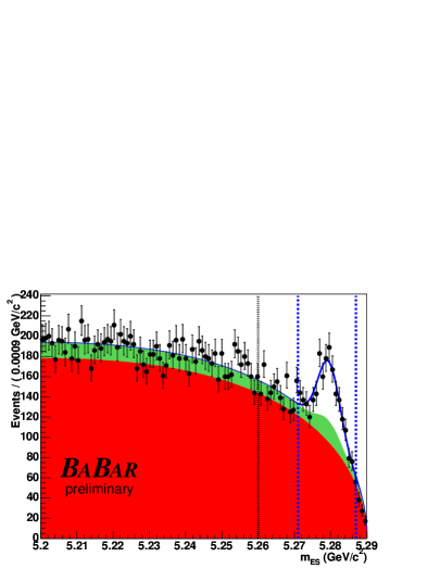
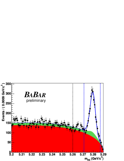
The distribution for events in the signal strip is used to determine the number of and signal events in the signal box. The signal component is modeled by a double Gaussian function with parameters obtained from phase-space MC. These parameters are fixed except for the mean of the core Gaussian. The continuum background is modeled using the experimentally motivated ARGUS function [9] with the endpoint fixed to the beam energy while the shape parameter is allowed to float. Finally, the background is modeled with an ARGUS function plus a Gaussian to account for peaking backgrounds. All parameters of the component, including the amount of peaking and nonpeaking background, are obtained and fixed from the MC simulation. The fraction of signal and events is allowed to float. Figure 2 shows the projections of fits to the data for both and . The per degree of freedom for these projections is 0.83 (1.13) for (). For the total number of events in the signal box is 2407; for the total number of events in the signal box is 3174. The extracted fractions of signal, continuum and backgrounds are given in Table 2.
| Total Events | 2407 | 3174 |
|---|---|---|
| Fraction of Events | ||
| Signal | 0.159 0.021 | 0.467 0.021 |
| background | 0.758 0.018 | 0.430 0.014 |
| background | 0.083 0.010 | 0.103 0.006 |
6 Dalitz Amplitude Analysis
In terms of a Dalitz-plot analysis of the -meson decay to the final state (where or ) a number of intermediate states contribute and the total rate can be represented in the form:
| (1) |
where and are the invariant masses squared of pairs of final state particles. In the case of , and ; for , and . The amplitude for a given decay mode is , where and are the unknown real parameters of each partial decay mode, while describes the dynamics of the amplitudes. These consist of a product of the invariant mass and angular distribution probabilities:
| (2) |
where is the resonance mass distribution and is the angular probability distribution. The angle is defined as the angle between the momentum vector of one of the resonance daughters in the resonance rest-frame and the momentum vector of the resonance in the rest-frame.
To fit the data in the signal box, we define an unbinned likelihood function for one event to have the form shown in Eq. 6. The fit is performed allowing the amplitude magnitudes () and the phases () to vary.
where
-
•
and are the invariant mass-squared values of the daughter pairs (1,3) and (2,3);
-
•
is the number of resonant and nonresonant contributions to the plot;
-
•
is the dynamical part of the amplitude of the resonant or nonresonant contribution ;
-
•
and are the real parameters to be determined ();
-
•
is the reconstruction efficiency defined for all points in the Dalitz plot;
-
•
is the distribution of continuum background;
-
•
is the distribution of background; and
-
•
and are the fractions of continuum and background events, respectively. They are determined from the fit and MC, respectively, and are fixed in the amplitude fit.
The first term on the right-hand-side in Eq. 6 corresponds to the signal probability density function (PDF) multiplied by the signal fraction . Since we can always apply a common factor to both the numerator and demoninator of the signal PDF, this analysis will only be sensitive to relative phases and magnitudes, and hence it is possible to fix the magnitude and phase of one component ( for and for ).
As the choice of normalisation, phase convention and amplitude formalism may not always be the same for different experiments, fit fractions are presented instead of amplitude magnitudes to allow a more meaningful comparison of results. The fit fraction is defined as the integral of a single decay amplitude squared divided by the coherent matrix element squared for the complete Dalitz plot as shown in Eq. 4.
| (4) |
Note that the sum of these fit fractions is not necessarily unity due to the potential presence of net constructive or destructive interference.
7 Physics Results
7.1 Results
The nominal fit is performed with the resonances , , , , and a uniform nonresonant (NR) contribution. The masses and widths of the resonances are fixed to their world average values [10]. In this fit the is fixed to have a magnitude of 1 and its phase is set to 0, since this is the dominant contribution to the Dalitz plot, and this choice reduces the statistical uncertainties for the other fitted components. We model all the resonances using relativistic Breit–Wigner lineshapes with Blatt–Weisskopf barrier factors [11] except for the , which is modeled with a Flatté lineshape [12] (to account for its coupled-channel behaviour due to the fact that it can decay to or ). The nonresonant component is assumed to be uniform in phase space. The preliminary results of the nominal fit to the 2407 events in the signal box can be seen in Table 3, along with the total branching fraction (BF) and the average efficiency across the Dalitz plot weighted by the fitted signal distribution.
| Average Efficiency (%) | |
|---|---|
| Total BF () | |
| Component | Fit Result |
| Fit Fraction (%) | |
| Phase | 0.0 (Fixed) |
| Fit Fraction (%) | |
| Phase | |
| Fit Fraction (%) | |
| Phase | |
| Fit Fraction (%) | |
| Phase | |
| NR Fit Fraction (%) | |
| NR Phase |
Figure 3 shows the mass projection plots for the nominal fit. The four resonant contributions plus the single uniform phase-space nonresonant model are able to adequately describe the data within the statistical uncertainties.
Further fits are performed to the data by removing one two-body component at a time from the nominal model; the results are shown in Table 4. Removing the , or components give significantly worse fit results. The omission of the and nonresonant amplitudes give values of the remaining fitted components that are close to their nominal values.
Recent experimental results from collisions at BES [13] show evidence of a low-mass pole in data for , known as the . Analysis of data from the E791 experiment for [16] show similar results. Also a large concentration of events in the S-wave channel has been seen in the region around MeV in collisions [14]. This pole is predicted from models based on chiral perturbation theory [15], in which the resonance parameters are MeV.
Consequently the resonance is predicted in decays. For this Dalitz-plot analysis the resonance is modeled using the parameterisation suggested by Bugg [17]. The result of the Dalitz-plot fit is shown in Table 5. It can be seen that the inclusion of the slightly changes the contributions of the other resonant components and also affects the phase of the nonresonant amplitude, but all results are consistent with those from the nominal fit, within the statistical uncertainties.
Table 5 also shows the preliminary results of the fit to the data when we add the and resonances to the model. Both contributions are found to be negligible.
| Nominal | No | No | No | No | No NR | |
| — | 94.3 | 8.0 | 1.7 | 18.9 | 2.8 | |
| Fit Fraction (%) | — | |||||
| Fit Fraction (%) | — | |||||
| Phase | (Fixed) | — | ||||
| Fit Fraction (%) | — | |||||
| Phase | — | |||||
| Fit Fraction (%) | — | |||||
| Phase | — | |||||
| NR Fit Fraction (%) | — | |||||
| NR Phase | — |
| Nominal | With | With | With | |
| — | -3.9 | -0.1 | 0.0 | |
| Fit Fraction (%) | ||||
| Fit Fraction (%) | ||||
| Phase | ||||
| Fit Fraction (%) | ||||
| Phase | ||||
| Fit Fraction (%) | ||||
| Phase | ||||
| NR Fit Fraction (%) | ||||
| NR Phase | ||||
| Fit Fraction (%) | — | — | — | |
| Phase | — | — | — | |
| Fit Fraction (%) | — | — | ||
| Phase | — | — | ||
| Fit Fraction (%) | — | — | — | |
| Phase | — | — | — |
7.2 Results
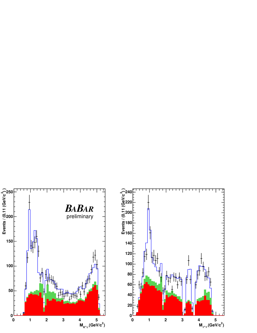
The expected significant contributions to the Dalitz plot can be identified from previous studies of this final state. Our model includes the following resonances: , , , , and a nonresonant amplitude. The masses and widths of the resonances are fixed to their world average values [10]. In the fits we use as the reference component and hence its magnitude and phase are fixed to 1 and 0, respectively. We use the same lineshapes described in Sec. 7.1 to model the resonance dynamics, except for , where we use the LASS amplitude model. The dynamics of the S-wave are not very well established and form an area of some disagreement within the community. Some favor the existence of the pole [17], whilst others strongly oppose it. All, however, agree that there is strong evidence of resonant behavior around 1430 , the . The LASS experiment studied scattering and as part of this study produced a description of the S-wave that consists of a resonant part, the , and an effective-range term [18, 19]. This amplitude is only measured up to around 2 in mass, and so we curtail the effective-range term at the lower edge of the veto. Since the LASS amplitude contains both a resonant and nonresonant part, the results for are not purely due to this resonance, but to the S-wave as a whole. This model, with five two-body components plus a uniform nonresonant component, with the LASS amplitude for the will be referred to as the “nominal” model.
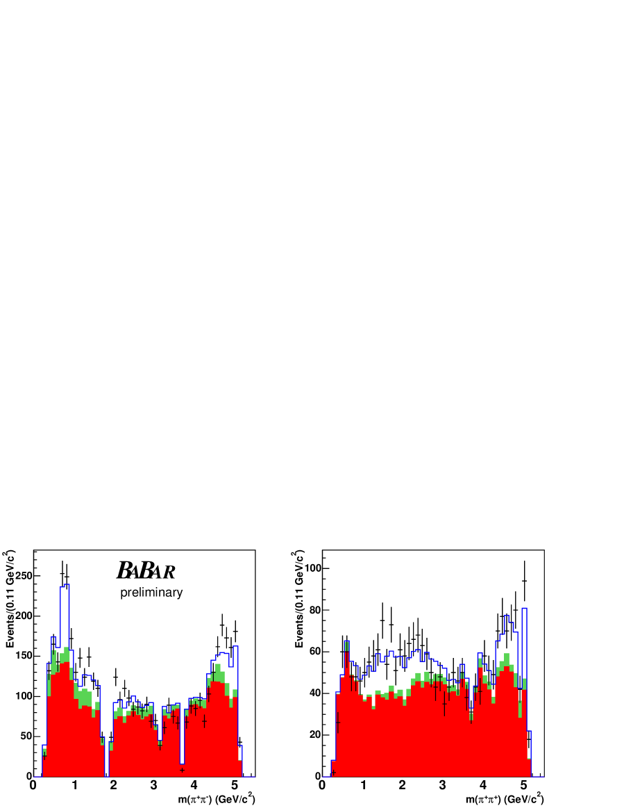
The nominal fit shows very good agreement with the data; a comparison can be seen in Figure 4. The preliminary results of the nominal fit to the 3174 events in the signal box can be seen in Table 6 along with the total branching fraction (BF) and the average efficiency across the Dalitz plot weighted by the fitted signal distribution. We have also used a relativistic Breit-Wigner or a Flatté lineshape for the resonance with and without the addition of a resonance, as suggested in Ref [17], to model the S-wave but found the fits to be poor representations of the data.
| Average Efficiency (%) | |
|---|---|
| Total BF () | |
| Component | Fit Result |
| Fit Fraction (%) | |
| Phase | 0.0 (Fixed) |
| Fit Fraction (%) | |
| Phase | |
| Fit Fraction (%) | |
| Phase | |
| Fit Fraction (%) | |
| Phase | |
| Fit Fraction (%) | |
| Phase | |
| NR Fit Fraction (%) | |
| NR Phase |
We refit the data removing each component in turn and find, in each case, that the fit worsens considerably. In some cases the parameters of the other components can vary dramatically. Table 7 details the results of these omission tests. We also test for the possibility that there are further resonances in the Dalitz plot by repeating the fit using the nominal model but adding an additional component. The possible additional states we test for are the , and resonances in the mass spectrum and the , and resonances in the mass spectrum. The results of these fits are shown in Table 8. In all cases the is slightly better than in the original fit. These checks are performed only on the sample.
| Nominal | No | No | No | No | No | No NR | |
| () ((nominal)) | — | 55.4 | 156.9 | 25.0 | 79.9 | 17.0 | 21.5 |
| Fit Fraction (%) | — | ||||||
| Fit Fraction (%) | — | ||||||
| Phase | — | ||||||
| Fit Fraction (%) | — | ||||||
| Phase | — | ||||||
| Fit Fraction (%) | — | ||||||
| Phase | (Fixed) | — | |||||
| Fit Fraction (%) | — | ||||||
| Phase | — | ||||||
| NR Fit Fraction (%) | — | ||||||
| NR Phase | — |
| Nominal | With | With | With | With | With | With | |
| () ((nominal)) | — | ||||||
| Fit Fraction (%) | |||||||
| Fit Fraction (%) | |||||||
| Phase | |||||||
| Fit Fraction (%) | |||||||
| Phase | |||||||
| Fit Fraction (%) | |||||||
| Phase | |||||||
| Fit Fraction (%) | |||||||
| Phase | |||||||
| NR Fit Fraction (%) | |||||||
| NR Phase | |||||||
| Fit Fraction (%) | — | — | — | — | — | — | |
| Phase | — | — | — | — | — | — | |
| Fit Fraction (%) | — | — | — | — | — | — | |
| Phase | — | — | — | — | — | — | |
| Fit Fraction (%) | — | — | — | — | — | — | |
| Phase | — | — | — | — | — | — | |
| Fit Fraction (%) | — | — | — | — | — | — | |
| Phase | — | — | — | — | — | — | |
| Fit Fraction (%) | — | — | — | — | — | — | |
| Phase | — | — | — | — | — | — | |
| Fit Fraction (%) | — | — | — | — | — | — | |
| Phase | — | — | — | — | — | — |
8 Systematic Studies
The charged particle tracking and particle identification uncertainties are 2.4% and 3.0%, respectively. There are also global systematic errors in the efficiencies due to the criteria applied to the event-shape variables (1.0%) and to and (1.0%). We also take into account the statistical uncertainty on the efficiency (due to the weighting by the amplitude model) for the individual and total branching fraction results (7% for , 6% for ). The uncertainty in the number of events is evaluated to be 1.1%.
The systematic error on the efficiency variation across the Dalitz plot is calculated by performing a series of fits to the data where we vary the contents of each bin in the efficiency histogram according to binomial errors. This introduces an absolute uncertainty of to for the phases, and a fractional uncertainty of % to for the fit fractions. However, for the average efficiency, and hence for the total branching fraction, this is a very small effect, evaluated as 0.1%.
The systematic uncertainty introduced by the background and background has two components, each of which can potentially affect the fitted magnitudes and phases differently. The first component arises from the uncertainty in the overall normalisation of these backgrounds, whilst the second component arises from the uncertainty on the shapes of the background distributions in the Dalitz plot. The uncertainties on the fit fractions and phases due to the normalisation uncertainty are estimated by varying the measured background fractions in the signal box by their statistical errors. The maximum associated absolute uncertainty for the phase is () for () due to the background normalisation uncertainty and due to the background normalisation uncertainty. These uncertainties are added in quadrature. The fit fractions are affected in a less uniform manner, with relative uncertainties in the range % to % (% to %) for (). The uncertainties on the fit fractions and phases due to the Dalitz-plot background distribution uncertainty is estimated in the same way as the efficiency variation, namely varying the contents of the histogram bins in accordance with their Poisson errors. To be conservative, each phase for has been given an associated uncertainty of 0.1 due to the background distribution uncertainty and 0.1 due to the background distribution uncertainty, which are then added in quadrature. For the variations between modes are larger and each mode is therefore treated individually. The range of uncertainties in the phases is to due to background and to due to background, which are again added in quadrature. The fit fractions are affected in a less uniform manner, with the relative uncertainties ranging from % to % (% to %) for ().
Possible biases due to the fitting procedure are investigated using extensive Monte Carlo simulations. We assign an absolute systematic error up to 3% for the fit fractions and 0.1 for the phases.
9 Summary
Tables 3 and 6 show the preliminary results from the nominal fits together with their statistical and systematic errors.
For the decay the nominal fit to the Dalitz plot is performed with the resonances , , , and a uniform nonresonant contribution. The total branching fraction is consistent with the previously measured value [2, 10]. We can estimate the branching fraction of by multiplying its fit fraction by the total branching fraction for . We find this to be , which is consistent with the previously measured value [20, 10]. The removal of any of the fit components gives worse likelihood values, especially for the , and resonances. It is found that the and resonances have no contribution to this Dalitz plot, while there is some evidence for a contribution from the .
For the decay the nominal fit to the Dalitz plot is performed with the resonances , , , , , a uniform nonresonant component and the LASS parameterization of the scalar component of the spectrum. The total branching fraction result is consistent with the previously measured value [2, 10]. We can estimate the branching fraction of by multiplying its fit fraction by the total branching fraction for . This yields a value of , which is smaller than that reported by earlier analyses that do not fit over the full Dalitz region but is consistent with the Dalitz analysis reported by Belle [4]. The resonance behavior around is successfully modeled with the LASS parameterization of the S-wave. The removal of any of the fit components results in a significant worsening of the fit likelihood and a large change in one or more of the remaining amplitudes. Addition of further resonances (, , , , or ) does not cause a significant change in the fit likelihood, and in most cases the extra component is measured to be compatible with having zero fit fraction. In addition, their presence in the fit does not significantly alter any of the other parameters and consequently has no significant effect on the fit fractions of the original components. The fit is stable with respect to different parameterizations of the Flatté line shape of the .
Future iterations of the analysis will use the information from the separate and samples to make measurements of the charge asymmetries of the various intermediate decay modes, potentially allowing observation of direct violation.
10 Acknowledgments
We are grateful for the extraordinary contributions of our PEP-II colleagues in achieving the excellent luminosity and machine conditions that have made this work possible. The success of this project also relies critically on the expertise and dedication of the computing organizations that support BABAR. The collaborating institutions wish to thank SLAC for its support and the kind hospitality extended to them. This work is supported by the US Department of Energy and National Science Foundation, the Natural Sciences and Engineering Research Council (Canada), Institute of High Energy Physics (China), the Commissariat à l’Energie Atomique and Institut National de Physique Nucléaire et de Physique des Particules (France), the Bundesministerium für Bildung und Forschung and Deutsche Forschungsgemeinschaft (Germany), the Istituto Nazionale di Fisica Nucleare (Italy), the Foundation for Fundamental Research on Matter (The Netherlands), the Research Council of Norway, the Ministry of Science and Technology of the Russian Federation, and the Particle Physics and Astronomy Research Council (United Kingdom). Individuals have received support from CONACyT (Mexico), the A. P. Sloan Foundation, the Research Corporation, and the Alexander von Humboldt Foundation.
References
- [1] Belle Collaboration, K. Abe et al., Phys. Rev. D 65, 092005 (2002)
-
[2]
BABAR Collaboration, B. Aubert et al.,
presented at FPCP 2002, hep-ex/0206004;
BABAR Collaboration, B. Aubert et al., Phys. Rev. Lett. 91, 051810 (2003) - [3] Belle Collaboration, K. Abe et al., Phys. Rev. D 69, 012001 (2004)
- [4] Belle Collaboration, K. Abe et al., presented at HEP 2003, BELLE-CONF-0338
- [5] BABAR Collaboration, B. Aubert et al., “The BABAR Detector,” Nucl. Instr. Meth. A 479, 1 (2002)
- [6] PEP-II Conceptual Design Report, SLAC-R-418 (1993)
-
[7]
R.A. Fisher,
Annals Eugen. 7, 179 (1936);
G. Cowan, Statistical Data Analysis, (Oxford University Press, 1998), p51 - [8] CLEO Collaboration, D. M. Asner, et al., Phys. Rev. D 53, 1039 (1996)
- [9] ARGUS Collaboration, H. Albrecht, et al., Z. Phys. C48, 543 (1990)
- [10] Particle Data Group, S. Eidelman et al., Phys. Lett. B 592, 1 (2004)
- [11] J. Blatt and V. Weisskopf, “Theoretical Nuclear Physics”, John Wiley and Sons, New York, 1956.
- [12] S.M. Flatté, Phys. Lett. B 63, 224 (1976)
- [13] BES Collaboration, “The pole in ”, submitted to Phys. Lett. B , hep-ex/0406038
- [14] D. Alde et al., Phys. Lett. B 397, 350 (1997)
- [15] G. Colangelo et al., Nucl. Phys. B 603, 125 (2001)
- [16] E791 Collaboration, E.M. Aitala et al., Phys. Rev. Lett. 86, 770 (2001)
- [17] D.V. Bugg, Phys. Lett. B 572, 1 (2003)
- [18] D. Aston et al., Nucl. Phys. B 296, 493 (1988)
- [19] W.M. Dunwoodie, Private Communication.
- [20] BABAR Collaboration, B. Aubert et al., Phys. Rev. Lett. 93, 051802 (2004)