Cracow 2004

PER ASPERA AD ASTRA

Despite the fact that Bremsstrahlung radiation has been observed many years ago, it is still the subject of interest of many theoretical and experimental groups. Due to the high sensitivity of the $NN~{}\to~{}NN\gamma$ reaction to the nucleon – nucleon potential, Bremsstrahlung radiation is used as a tool to investigate details of the nucleon – nucleon interaction. Such investigations can be performed at the cooler synchrotron COSY in the Research Centre Jülich, by dint of the COSY–11 detection system.
For the first time at the COSY–11 experiment signals from $\gamma$ – quanta were observed in the time – of – flight distribution of neutral particles measured with the neutral particle detector.
In this thesis the results of the identification of Bremsstrahlung radiation emitted via the $dp~{}\to~{}dp\gamma$ reaction in data taken with a proton target and a deuteron beam are presented and discussed.
The time resolution of the neutral particle detector and its timing calibration are crucial for the identification of the $dp~{}\to~{}dp\gamma$ reaction. Therefore, methods of determining the relative timing between individual modules – constituting the neutron detector – and of the general time offset with respect to the other detector components are described. Furthermore the accuracy of the momentum determination of the registered neutron which defines the precision of the event reconstruction was extracted from the data.

Chapter 1 Introduction

In collisions between nucleons electromagnetic radiation can be emitted due to the rapid change of the nucleon velocity. This radiation is referred to as bremsstrahlung radiation. Although it has been observed many years ago, it is still the subject of interest of many experimental and theoretical groups [1, 2, 3, 4]. Due to the high sensitivity of the $NN~{}\to~{}NN\gamma$ reaction to the nucleon–nucleon potential, bremsstrahlung radiation is used as a tool to investigate details of the NN interaction and to discriminate between various potential models [1, 2].

Such investigations can be performed at the cooler synchrotron COSY in the Research Center Jülich, by means of the facilities installed there like the internal COSY–11 detection setup. Although the COSY–11 facility is designed for threshold meson production covering a small solid angle in the laboratory system the special configuration allows also the study of reaction channels at high excess energies. The main aim of this thesis is an identification of bremsstrahlung radiation in a data sample taken by the COSY–11 collaboration during a measurement in January 2003 [5, 6]. The measurement was carried out at a hydrogen cluster target [7] using a deuteron beam with a momentum of 3.204 GeV/c. The registration of gamma quanta became possible because the COSY–11 detection system has been extended by a neutral–particle–detector. This detector enables not only to measure the bremsstrahlung radiation created in the collision of nucleons but also opens wide possibilities to investigate the isospin dependence of the meson production in the hadronic interactions [8]. For example at present the COSY–11 facility permits to investigate $\eta$–meson production in proton–proton and proton–neutron collisions [9, 10]. Neutrons and gamma quanta registered in the neutral–particle–detector are identified via the time–of–flight on the 7 m distance between the target and the detector. In case of a neutron the time–of–flight and the hit position enables to determine its four–momentum vector. Since the time resolution of the detector and its timing calibration are crucial for the identification of the studied reactions, the data analysis of the $dp~{}\to~{}dp\gamma$ reaction will be preceded by the detailed presentation of the method used for the time calibration of this detector.

The present thesis is divided into six chapters. The second chapter — following the introduction — describes briefly the motivations to investigate the $NN~{}\to~{}NN\gamma$ process, in particular, in view of the study of the proton–$\eta$ interaction by the COSY–11 group.

Description of the detection system, with a special emphasis on the structure of the neutron detector and the basis of its functioning will be presented in the third chapter.

The fourth chapter is devoted to the time calibration of the neutral–particle–counter. The method of determining the relative timing between the individual modules and the general time offset with respect to the other detectors will be depicted. This chapter describes also the determination of the momentum resolution of the registered neutrons.

The results of the identification of the $dp~{}\to~{}dp\gamma$ reaction in data taken in January 2003 are presented in the fifth chapter, where also a detailed description of the data analysis is included.

The sixth chapter comprises summary and perspectives, in particular a possibility to study the pentaquark state $\Theta^{+}$ at the COSY–11 facility is discussed.

Chapter 2 Motivation

For many years experimental and theoretical studies have been devoted to distinguish among various potential models and estimate of the off-shell amplitudes. The idea of using nucleon–nucleon bremsstrahlung as a tool for investigating this problem has attracted attention since calculations of the cross sections of the $NN~{}\to~{}NN\gamma$ reaction are highly sensitive to the $NN$ potential.

We would like to study this process also in view of another important issue related to the $\eta$–proton interaction.

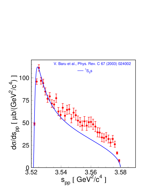
Figure 2.1: Differential cross section for the $p~{}p~{}\to~{}p~{}p~{}\eta$ reaction as a function of the invariant mass of proton–proton system. Data are from ref. [11] and the line corresponds to the model of reference [12]. Picture adapted from [11].

Figure 2.1 shows a differential cross section for the $pp~{}\to~{}pp\eta$ reaction as a function of the invariant mass of the proton–proton system. The measurement has been performed at an excess energy of Q = 15.5 MeV. The theoretical description does not agree with data in the whole range of invariant mass of the proton–proton system. It has been pointed out that the difference between the data and the theoretical predictions originates from proton–$\eta$ interaction in the final state. In order to prove that this conclusion does not depend on the applied model it would be desirable to compare this distribution with the one obtained for the $ppX$ system, where $X$ does not interact strongly with protons. Therefore best suited for this purpose would be the $pp\gamma$ system. Let us assume, that the differential cross section for the $pp~{}\to~{}pp\gamma$ reaction as a function of proton–gamma invariant mass are determined. If the theoretical model, used for the calculations presented by the solid line in figure 2.1 were in perfect agreement with those data, it would corraborate the assertion that the disagreement between data and theory in the $pp\eta$ case is due to the p–$\eta$ interaction.
Studies of the $pp$–bremsstrahlung by means of the COSY–11 facility haven’t been performed, but production of bremsstrahlung radiation in proton–proton collisions was investigated at the COSY–TOF facility [3]. Data have been taken at a proton beam momentum of 797 MeV/c using a wide angle spectrometer. At the COSY–11 facility as a first step of investigations of the bremsstrahlung radiation the $dp~{}\to~{}dp\gamma$ reaction is studied, and the main point of the present work is an identification of dp$\gamma$ events in data taken during the experiment devoted to the measurement of the $\eta$–meson production in deuteron–proton collisions.

Figure 2.2: Total cross section for the $dp~{}\to~{}dp\gamma$ reaction as a function of the excess energy. Original data are taken from [4].

A similar experiment — measurement of the $dp~{}\to~{}dp\gamma$ reaction — has been performed by the WASA/PROMICE collaboration at the storage ring CELSIUS, with deuteron beam energies between 437 MeV and 559 MeV. In these studies angular and spectral distributions are divided into two groups that can be attributed to a quasifree $np~{}\to~{}np\gamma$ process, and to a gamma production process with all three nucleons involved, viz: $dp~{}\to~{}dp\gamma$. The results of these investigations — the total cross section for the $dp~{}\to~{}dp\gamma$ reaction — are given in figure 2.2.

In this work the feasibility of the bremsstrahlung measurement at the COSY–11 detection setup will be proven, and as soon as the analysis is finished the total cross section data–base for the $dp~{}\to~{}dp\gamma$ reaction (fig. 2.2) will be extended by one point at Q = 557 MeV.

Chapter 3 Experimental setup

3.1 COSY–11 facility—general remarks

The experiment described in this thesis has been performed at the COSY–11 facility [13], an internal magnetic spectrometer installed at the cooler synchrotron COSY in Jülich [14]. The COSY–11 detection system is schematically depicted in figure 3.1. Details of the functioning of all detector components and the method of measurement can be found in references [13, 15, 16]. Therefore, here the used experimental technique will be only briefly presented.

The synchrotron accelerates protons and deuterons up to a momentum of 3.4 GeV/c. At the highest momentum a few $10^{10}$ accelerated particles pass through the target $\sim 10^{6}$ times per second.
The hydrogen ($H_{2}$) or deuteron ($D_{2}$) cluster target (see figure 3.2) is installed in front of the dipole magnet. The positively charged products of the reaction are bent in the magnetic field of the dipole and leave the vacuum chamber through thin exit foils, whereas the beam — due to the much larger momentum — remains on its orbit inside the ring. The charged ejectiles are detected in drift chambers (D1, D2, D3) [13] and scintillator hodoscopes (S1, S2, S3) [13, 15]. Neutrons and gamma quanta are registered in the neutron detector (N). In order to separate neutrons and gamma quanta from charged particles veto detector (V) is used. An array of silicon pad detectors ($Si_{spec}$) is used for the registration of the spectator protons. Protons scattered under large angle are measured in another position sensitive silicon pad detector $(Si_{mon})$.

The experiments performed at COSY–11 base on the measurement of four-momenta of the outgoing particles. Unregistered short lived mesons and hyperons are identified via the missing mass technique.

For each charged particle, which gave signals in drift chambers, the momentum vector can be determined. First the trajectories of the particles are reconstructed [17], and then knowing the magnetic field of the dipole, the momentum vector is reconstructed. In case of two close tracks, the information about the energy loss from S1, S2, and S3 is used to inspect the efficiency of the track reconstruction. Particle’s velocity determination is based on the time-of-flight measurement between S1 (or S2) and S3 detectors. Knowing the velocity and the momentum of the particle, its mass can be calculated, and hence the particle can be identified. After the particle identification the time of the reaction at the target is obtained from the known trajectory, velocity, and the time measured by the S1 detector. The neutron detector delivers the information about the time at which the registered neutron or gamma quanta induced a hadronic or electromagnetic reaction.

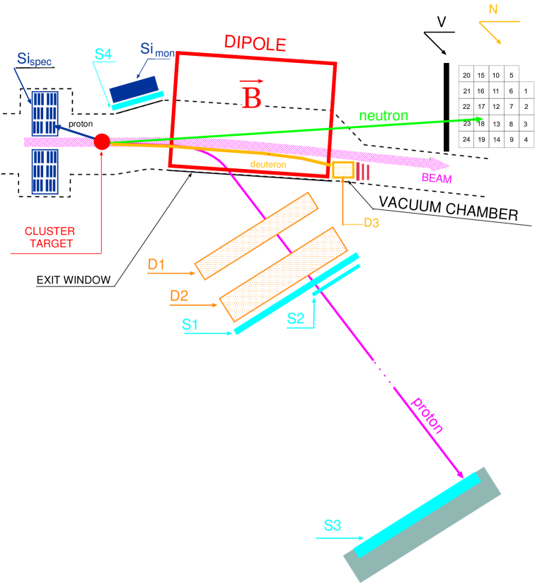
Figure 3.1: Scheme of the COSY–11 detection system. Protons are registered in two drift chambers D1, D2 and in the scintillator hodoscopes S1, S2, S3. An array of silicon pad detectors $(Si_{spec})$ is used for the registration of the spectator protons. Neutrons are registered in the neutron modular detector (N). In order to distinguish neutrons from charged particles a veto detector (V) is used. Deuterons with larger momentum are registered in deuteron chamber D3.

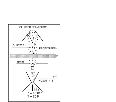
Figure 3.2: Schematic view of the cluster target.

The time of the reaction combined with this information allows to calculate the time–of–flight (TOF^N) of the neutron (or gamma) between the target and the neutron detector, and — in case of neutrons — to determine the absolute value of the momentum (p) what can be expressed as:

$$p=m\cdot{l\over{TOF^{N}}}\cdot{1\over{\sqrt{1-({l\over{TOF^{N}}})^{2}}}},$$ (3.1)

where m denotes the mass of the particle, $l$ stands for the the distance between the target and the neutron detector and $TOF^{N}$ is the time–of–flight of the particle.

In order to calculate the four–momentum of the spectator proton — in case of quasi–free reactions with proton beam and deuteron target — its kinetic energy (T) is directly measured as the energy loss in the silicon detector $(Si_{spec})$. Knowing the proton kinetic energy one can calculate its momentum using the following relationship:

$$p=\sqrt{{(T+m)}^{2}-m^{2}},$$ (3.2)

where $m$ denotes the proton mass, and $T$ is the kinetic energy. In case of the measurements with deuteron beam and proton target the trajectory of the spectator proton may be reconstructed from signals from the drift chambers D1 and D2 and hence in this case its momentum can also be determined.

To evaluate the luminosity, the elastically scattered protons are measured at the same time. With one proton detected in the drift chambers and scintillator hodoscopes and the other proton in the silicon detector $Si_{mon}$ resulting in the determination of the hit position, the elastically scattered protons can be well separated.

3.2 Functioning of the neutron detector

In this section I would like to emphasize the neutron detector, since the time calibration of this detector constitutes one of the main goals of this thesis.

Previously, the neutron detector was built out of 12 detection units, with light guides and photomultipliers mounted on one side of the module. In order to improve the time resolution of the detector additional light guides and photomulipliers were installed, such that the light signals from scintillation layers are read out at both sides of the module. The present neutron detector consists of 24 modules, like the shown in figure 3.3. Each module is built out of eleven plates of scintillator material with dimensions 240 mm x 90 mm x 4 mm interlaced with eleven plates of lead with the same dimensions. The scintillators are read out at both edges of the module by light guides — made of plexiglass — whose shape changes from rectangular to cylindrycal, in order to accumulate the produced light on the circular photocathode of a photomultiplier.

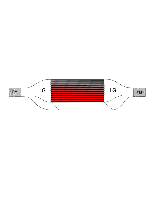
Figure 3.3: Schematic view of a single module of the neutron detector. LG and PM denote light guides and photomultipliers, respectively. Picture is taken from [18].

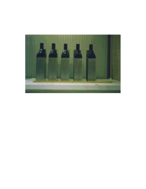
Figure 3.4: Photo of single modules of the neutron detector, at the stage when the scintillator/lead structure was well visible.

The neutron detector is positioned at a distance of 7 m behind the target in the configuration schematically depicted in figure 3.5. As can be deduced from figure 3.6 the maximum efficiency, for a given total thickness, for the registration of the neutron — in the kinetic energy range of interest for the COSY–11 experiments ($\sim$ 300 MeV – $\sim$ 700 MeV) — would be achieved for the homogeneous mixture of lead and scintillator. In order to optimize the efficiency and the cost of the detector the plate thickness has been chosen to be 4 mm. This results in an efficiency which is only few per cent smaller than the maximum possible.

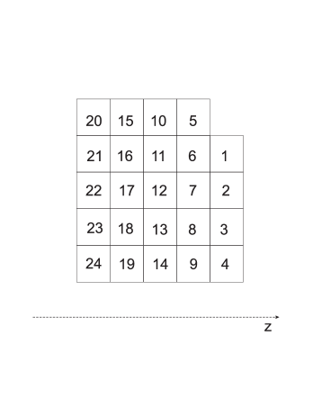
Figure 3.5: Schematic view of the neutron detector from above. The squares with numbers represent single detection modules. The z axis is defined by the beam direction.

Figure 3.6: Calculated efficiencies of the 20 cm thick neutron detector as a function of neutron kinetic energy for various layer thicknesses of the scintillator and lead plates. The solid line with triangles is for pure scintillator. Diamonds denote a layer thickness of 0.5 mm, closed circles of 2 mm, open circles of 5 mm, and crosses of 25 mm. The figure has been adapted from [19].

The functioning of the detector was already confirmed in experiments carried out with a deuteron beam and hydrogen target. Figure 3.7 shows experimental distributions of the number of hits per individual detection unit, for neutral (left) and charged particles (right). As expected the counting rate of modules in the middle part of the detector is much higher than these for the modules on the edges. In particular the smallest rate is observed in modules No. 5, 10, 15, and 20, because this row is partly out of the geometrical acceptance of the dipole yoke. The number of hits per segment from experiment is in perfect agreement with the corresponding spectra which were simulated using a GEANT–3 code (see figure 3.8).

Figure 3.7: Number of hits per individual module. Experimental spectra obtained for neutral particles (left) and charged particles (right) are shown.

Figure 3.8: Number of hits per individual module from Monte-Carlo studies obtained for neutral particles (left) and charged particles (right). The simulation was performed for the $dp~{}\to~{}ppn_{sp}$ reaction taking into account reactions of the ejectiles with the dipole and all detector materials.

Chapter 4 Calibration of the neutron detector

The installation of the neutral particle detector at the COSY–11 facility enables to study a plethora of new reaction channels. This detector is designed to deliver the time at which the registered neutron or gamma quantum induced a hadronic or electromagnetic reaction, respectively. This information combined with the time of the reaction at target place — deduced using other detectors — enables to calculate the energy of the detected neutron. In this section a method of time calibration will be demonstrated and results achieved by its application will be presented and discussed. Information about the deposited energy is not used in the data analysis because the smearing of the neutron energy determined in this manner is by more than order of magnitude larger than this established from the time–of–flight method.

4.1 Time calibration of the neutron detector

4.1.1 Time signals from a single detection unit

As already discussed in section 3.2 the neutron detector at the COSY–11 facility is built out of 24 modules such as the one shown in the figure below.

The time ($T^{exp}$) from a single module is calculated as an average time measured by the upper and lower photomultiplier. Namely:

$$T^{exp}={{{T}^{up}_{TDC}+{T}^{dw}_{TDC}}\over 2},$$ (4.1)

where $T_{TDC}$ denote the time difference between the arrival of the photomultiplier and trigger signals to the Time–to–Digital–Converter (TDC).

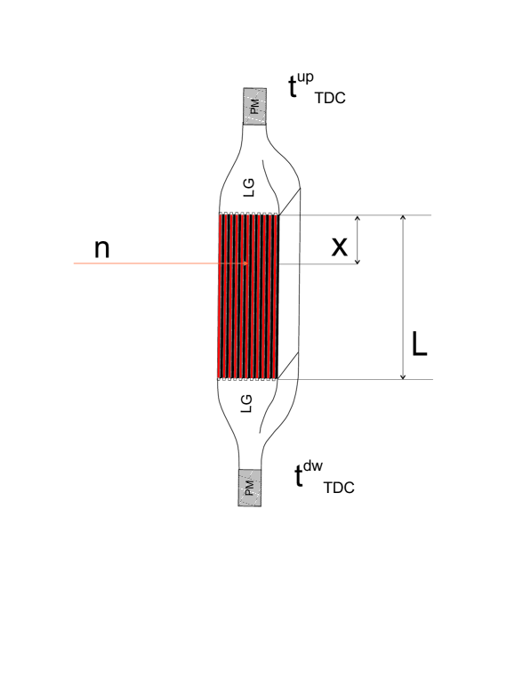
Figure 4.1: Definition of variables $x$ and $L$ used in the text. The scheme of the detection module is the same as in figure 3.3.

This can be expressed as:

$${T}^{up}_{TDC}={t}_{real}+\mbox{offset}^{up}+{{x}\over c_{L}}-T_{trigger},$$ (4.2)

$${T}^{dw}_{TDC}={t}_{real}+\mbox{offset}^{dw}+{{L-x}\over c_{L}}-T_{trigger},$$ (4.3)

where $L$ stands for the length of a single module, $x$ denotes the distance between the upper edge of the active part of the detector and the point at which a neutron induced the hadronic reaction, $t_{real}$ is the time at which the scintillator light was produced, $T_{trigger}$ represents the time at which the trigger signal arrives at the TDC converter, and c_L denotes the velocity of the light signal propagation inside the scintillator plates. The parameters offset^up and offset^dw denote the time of propagation of signals from the upper and lower edge of the scintillator to the TDC unit.

Applying equations 4.1, 4.2, and 4.3 one can calculate a relation between $T^{exp}$ and $t_{real}$:

$$T^{exp}=t_{real}+{{\mbox{offset}^{up}+\mbox{offset}^{dw}+{{L}\over c_{L}}}\over 2}-T_{trigger}=t_{real}+\mbox{offset}-T_{trigger}$$ (4.4)

The value of “offset” comprises all delays due to the utilized electronic circuits, and it needs to be established for each segment. It is worth to note, that this time of the neutron detector signal is independent of the hit position, as it can be deduced from equation 4.4 and was proven experimentally, and depends on the difference between the time of light generation and the trigger only.

4.1.2 Relative timing between modules

Instead of determining the value of “offset” from equation 4.4 for each detection unit separately, the relative timing between modules will be first established and then the general time offset connecting the timing of all segments with the other detectors of the COSY–11 setup will be found. In order to establish relative time offsets for all single detection units, distributions of time differences between neighbouring modules were derived from experimental data. A time difference measured between two modules can be expressed as:

$$\Delta_{ij}=T^{exp}_{i}-T^{exp}_{j}={t}_{i}^{real}-{t}_{j}^{real}+(\mbox{offset}_{i}-\mbox{offset}_{j}),$$ (4.5)

where $T^{exp}_{i}$ and $T^{exp}_{j}$ stand for the time registered by the $i^{th}$ and $j^{th}$ module, respectively. Example of ${\Delta}_{ij}$ spectra determined from a measurement carried out in January 2003 with a hydrogen target and a deuteron beam accelerated to the momentum of $p_{b}$ = 3.204 GeV/c are presented in figure 4.2. The time differences were calculated assuming that all constants (offset) are equal to zero (see eq. 4.5). One can note that the peaks are shifted and additionally the distributions contain long tails. The tails reflect the velocity distribution of the secondary particles. Corresponding spectra of time differences between the modules, shown in the figure 4.3, were generated using a GEANT–3 code. To produce these spectra the quasi–free $dp~{}\to~{}ppn_{sp}$ reaction has been simulated. The details are described in the appendix A. The values of the relative time offsets were determined using a dedicated program written in the Fortran 90 language [22, 23]. It adjusts values of offsets such that time differences obtained from experimental data and from simulation equals to each other for each pair of detection units. Furthermore, from the width of the spectra one can receive the information about the time resolution of a single module, which was found to be 0.4 ns [22].

Figure 4.2: Distribution of the time difference between the $6^{th}$ and the $11^{th}$, the $7^{th}$ and the $12^{th}$, and the $8^{th}$ and the $13^{th}$ module of the neutron detector, as determined before the calibration.

Figure 4.3: Simulated distribution of the time difference between the $6^{th}$ and the $11^{th}$, the $7^{th}$ and the $12^{th}$, and the $8^{th}$ and the $13^{th}$ module of the neutron detector.

-0.5cm

Figure 4.4: Distribution of the time difference between the $6^{th}$ and the $11^{th}$, the $7^{th}$ and the $12^{th}$, and the $8^{th}$ and the $13^{th}$ module of the neutron detector, as obtained after the calibration.

Figure 4.4 presents experimental distributions of time differences between neighbouring modules as determined after the calibration. Examining figure 4.3 and 4.4 it is evident that now the peaks are positioned precisely at the value expected from simulation.

4.1.3 General time offset

For the determination of the momentum of neutrons eg. in the analysis of reactions like $dp~{}\to~{}ppn\gamma$, the time between the reaction moment and the hit time in the neutron detector has to be determined for each event. The time of the reaction can be deduced from the time when the charged particle crosses the S1 detector (see fig. 3.1) assuming that this particles trajectory and velocity can be reconstructed. To perform the calculation of the time–of–flight between target and neutron counter a general time offset of the neutron detector with respect to the S1 detector has to be established. For this purpose the quasi–free $dp~{}\to~{}ppn_{sp}$ reaction will be used. In this type of reactions the proton bound in a deuteron scatters elastically on a target proton, whereas the neutron considered as a spectator does not interact with the proton, but escapes untouched and hits the neutron detector.

Data have been taken at a beam momentum of 3.204 GeV/c close to thereshold of the $dp~{}\to~{}dp\eta$ process. Events corresponding to the $dp~{}\to~{}ppn_{sp}$ reaction have been identified by measuring the outgoing charged as well as neutral ejectiles.

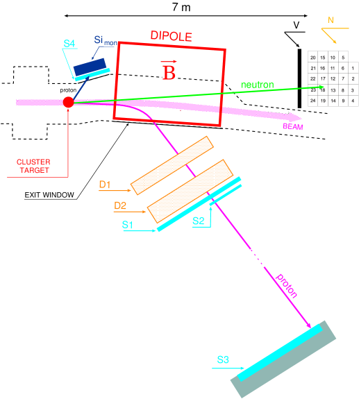
Figure 4.5: Schematic view of the COSY–11 detection system. Only detectors used for the measurement of elastic scattered protons and spectator neutrons are shown.

Fast protons are detected by means of the drift chambers (D) and scintillator hodoscopes (S1-S3). Protons scattered under large angles are measured in a position sensitive silicon detector $(Si_{mon})$. Neutrons are registered in the scintillator–lead sandwich detector (N).

The time-of-flight between the target and the neutron detector $({TOF}^{neut})$ is calculated as a difference between the time of the module in the neutron detector which fired as the first one ($t_{n}^{real}$) and the time of the reaction $(t^{real}_{r})$.

$${TOF}^{neut}=t_{n}^{real}-t^{real}_{r}$$ (4.6)

Time of the reaction is obtained from backtracking of protons through the known magnetic field and the time measured by the S1 detector ($T^{S1}$). Thus $t^{real}_{r}$ can be expressed as:

$$t^{real}_{r}=t_{S1}-TOF=T^{S1}-\mbox{offset}^{S1}+T_{trigger}-TOF,$$ (4.7)

where $TOF$ denotes the time–of–flight between the S1 counter and the target, and offset^S1 denotes all delays of signals from the S1 detector. Since time in the neutron detector reads:

$$t_{n}^{real}=T_{n}-\mbox{offset}^{N}+T_{trigger}$$ (4.8)

we have:

$${TOF}^{neut}=T_{n}+TOF-T^{S1}-\mbox{offset}^{N}+\mbox{offset}^{S1}=T_{n}+TOF-T^{S1}+\mbox{offset}^{G}$$ (4.9)

By offset^G the general time offset of the neutron detector in respect to S1 is denoted. In order to establish this global time offset, the time–of–flight spectrum derived from experimental data for the $dp~{}\to~{}ppn_{sp}$ reaction was compared with the corresponding distribution which was reconstructed from the signals simulated in the detectors (see figure 4.6 left). To arrive at the same statistic as was achieved in experiment, $8\cdot 10^{6}$ events for the $dp~{}\to~{}ppn_{sp}$ reaction were simulated using a GEANT–3 code. In the simulation the time resolution of a single module of $\sigma~{}=~{}0.4$ ns was taken into account.

Figure 4.6: (left) Time–of–flight distribution between the target and the neutron detector as obtained before the general time offset had been determined. The dashed histogram denotes the experimental data whereas the solid one depicts the result of the simulation. (right) Experimental time-of-flight distribution (dashed histogram) calculated between the target and the neutron detector with general time offset equal to 13.6 ns compared to the Monte–Carlo simulation (solid histogram). The latter was normalized in number of counts to the experimental data.

The simulated spectrum was normalized so that the integrals of both distributions are equal. With a general time offset of 13.6 ns the experimental distribution corresponds to the simulated one as shown in figure 4.6 (right). The main cause of the smearing of the considered time distribution is the Fermi momentum of the nucleon inside the deuteron. The time resolution and dimensions of the detector are of minor importance.

4.2 Momentum resolution

The experimental resolution of the missing mass determination eg. in the analysis of reactions like $pn~{}\to~{}pn\eta^{\prime}$ strongly rely on the accurate measurement of the momentum of the neutrons [9]. Therefore, the momentum resolution of the neutron detector has to be elaborated. After the neutron and gamma quanta are identified the momentum of neutrons is calculated from the time–of–flight between the target and the neutron detector according to the formula 3.1.

Monte Carlo studies of the $dp~{}\to~{}ppn_{sp}$ reaction have been performed in order to establish the momentum resolution of the neutron detector. Figure 4.7 presents the difference between the generated neutron momentum ($P_{gen}$) and the reconstructed neutron momentum from signals simulated in the detectors ($P_{rec}$).

$$\Delta P=P_{gen}-P_{rec}$$ (4.10)

The value of ($P_{rec}$) was calculated taking into account the time resolution of the neutron detector ($\sigma$ = 0.4 ns) as well as the time resolution of the S1 counter ($\sigma$ = 0.25 ns).

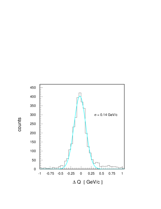
Figure 4.7: Difference between generated ($P_{gen}$) and reconstructed ($P_{rec}$) neutron momenta for the $dp~{}\to~{}ppn_{sp}$ reaction simulated at deuteron beam momentum of 3.204 GeV/c.

The distribution of $\Delta P$ was fitted by a Gaussian function resulting in a momentum resolution of $\sigma$(P) = 0.14 GeV/c. Consequently the fractional momentum resolution $\sigma$(P)/P for neutrons with momentum value of 1.6 GeV/c is equal to 8%. This fractional resolution changes with the momentum of the neutron (see Appendix B) and eg. for the neutrons produced at threshold for the $pn~{}\to~{}pn\eta$ reaction it amounts to 3$\%$.

Chapter 5 Analysis of the experimental data

For the first time at the COSY–11 experiments signals from $\gamma$–quanta were observed in the time–of–fligth distribution (for the neutral particles) measured between the target and the neutral particle detector. A corresponding spectrum is shown in figure 5.1(left). The data are from an experiment carried out using a deuteron target and a proton beam with a momentum of 2.075 GeV/c [9]. In addition to a broad distribution originating from neutrons, a sharp peak from ${\gamma}$ rays is seen at a value of about 25 ns. A Monte Carlo simulation performed for the $pn~{}\to~{}pn\eta$ reaction, which is one of the possible processes contributing to the neutron time-of-flight distribution, is shown in figure 5.1(right)

Figure 5.1: Time–of–flight distribution determined between the target and the neutron detector.
(left) Experimental spectra, and (right) Monte Carlo simulation. Figure adapted from [20]

In this chapter results of the analysis aiming for the identification of bremsstrahlung radiation in the data taken in January 2003 will be presented. The measurement was carried out with a deuteron beam and hydrogen cluster target at the cooler synchrotron COSY–Jülich by means of the COSY–11 detection system, and its primordial aim was to investigate the $dp~{}\to~{}dp\eta$ reaction close to the threshold [5]. The experiment was performed at four different deuteron beam momenta between $p_{beam}$ = 3.165 and 3.204 GeV/c. During the run with a beam momentum of $p_{beam}$ = 3.204 GeV/c, an additional trigger with neutron detector — referred to T8 — was set up for the registration of charged ejectiles in coincidences with neutrons or gamma quanta. These conditions can be written symbolically as:

$$T8={S1}_{\mu=2}\wedge N_{\mu\geq 2}\wedge S3_{\mu=1},$$

which means that two signals in the S1 detector, one signal in the S3 detector and, at least two signals in the neutron detector were demanded.

Possible reactions with gamma quanta in the final state can be divided into two groups, viz: free $dp~{}\to~{}dp\gamma$ and $dp~{}\to~{}^{3}He\gamma$ reactions, and quasi–free $dp~{}\to~{}dp_{sp}\gamma$, $dp~{}\to~{}pp\gamma n_{sp}$, $dp~{}\to~{}pn\gamma p_{sp}$ reactions. In case of quasi–free reactions one of the nucleons bound in a beam deuteron is treated as a spectator ($p_{sp},n_{sp}$) and does not take part in the reaction.

As a first step of the data analysis events with simultaneous signals in any of the drift chambers and the neutron detector were selected. Figure 5.2 presents the time–of–flight distributions between the target and the neutron detector obtained assuming that in coincidence with a neutral particle also a proton (left) or deuteron (right) was identified based on signals from drift chambers and scintillator hodoscopes. The signals from $\gamma$–quanta do not appear in the distributions which are predominantly due to quasi–free elastic $dp~{}\to~{}ppn_{sp}$ and $dp~{}\to~{}dn\pi^{+}$ reactions.

Figure 5.2: Experimental time–of–flight distributions determined between the target and the neutron detector obtained under the condition that additionally one proton (left) or one deuteron (right) was registered in drift chambers.

The charged ejectiles can be well identified as shown in the figure 5.3. Three clear peaks evidently visible in this figure correspond to the squared mass of pion, proton, and deuteron. The mass of the particle is calculated from its momentum — reconstructed from tracking back through magnetic field to the target point — and velocity determined from the time–of–flight measured between S1 and S3 detector.

Figure 5.3: Distribution of the squared mass of charged particles originating from the deuteron–proton reaction performed at a beam momentum of 3.204 GeV/c.

5.1 Identification of the $dp~{}\to~{}dp\gamma$ reaction

In order to identify the $dp~{}\to~{}dp\gamma$ reaction events with two tracks in drift chambers and a simultaneous signal in a neutron detector have been selected. In figure 5.4 squared mass of one particle is plotted versus squared mass of the other registered particle. Base on this figure measured reactions can be grouped according to the type of ejectiles.

Figure 5.4: Scatter plot of invariant masses determined for events with two charged particles measured in coincidence.

Thus reactions with two protons, proton and pion, proton and deuteron, and pion and deuteron can be cleary separated. Figure 5.5 shows the experimental distribution of the time–of–flight between the target and neutral–particle detector with the requirement that two charged particles were registered and that one of them was identified as a proton and the other as a deuteron. In this case due to the baryon number conservation, there is only one possible source of a signal in a neutron detector, namely a gamma quantum. In fact a clear peak around the time of 24.5 ns is visible, and this is just the value corresponding to the time–of–flight of light on a distance of 7m. The gamma quanta may originate from the bremsstrahlung reaction ($dp~{}\to~{}dp\gamma$) or from the decay of mesons produced eg. via $dp\to~{}dp\pi^{0}~{}\to~{}dp\gamma\gamma$ or $dp~{}\to~{}dp\pi^{0}\pi^{0}~{}\to~{}dp4\gamma$ reactions. It is possible to distiguish between these hypothesis calculating the missing mass produced in the $dp~{}\to~{}dpX$ reaction.

Figure 5.5: Time–of–flight distribution determined between the target and the neutron detector obtained under the assumption that additionally to a signal in the neutron detector, one proton and one deuteron were identified from the signals in the drift chambers.

Knowing the four momenta of a proton and a deuteron in the initial and final state, and employing the principle of momentum and energy conservation one can calculate the squared mass of the unmeasured particle or group of particles:

$$m_{x}^{2}=E_{x}^{2}-{\vec{p_{x}}}^{2}={(E_{b}+E_{t}-E_{d}-E_{p})}^{2}-{(\vec{p}_{b}+\vec{p}_{t}-\vec{p}_{d}-\vec{p}_{p})}^{2}$$ (5.1)

where,
$E_{b},\vec{p}_{b}$ is the energy and momentum of deuteron beam,
$E_{t},\vec{p}_{t}$ is the energy and momentum of proton target,
$E_{d},\vec{p}_{d}$ is the energy and momentum of outgoing deuteron, and
$E_{p},\vec{p}_{p}$ is the energy and momentum of outgoing proton.

Figure 5.6 shows the squared missing mass distribution as obtained for the $dp~{}\to~{}dpX$ reaction. A significant peak around 0 $MeV^{2}/c^{4}$ — the squared mass of the gamma quantum — constitutes an evidence for events associated to the deuteron–proton bremsstrahlung ($dp\gamma$). In addition a broad structure at higher masses originating from two pions emitted from the reaction $dp~{}\to~{}dp\pi^{0}\pi^{0}$ is visible.

Figure 5.6: Squared missing mass distribution for the $dp~{}\to~{}dpX$ reaction.

One of the most important information is the energy spectrum of the gamma quanta. The energy of gamma quanta can be measured with a very poor accuracy, however it can be calculated using a simple relation, after selecting events corresponding to the $dp~{}\to~{}dp\gamma$ reaction, namely:

$$E_{\gamma}=E_{b}+E_{t}-E_{d}-E_{p}$$ (5.2)

where,
$E_{b}$ is the energy of deuteron beam,
$E_{t}$ is the energy of proton target,
$E_{d}$ is the energy of outgoing deuteron, and
$E_{p}$ is the energy of outgoing proton.

Figure 5.7 shows the determined spectrum. One sees that the registered gamma quanta populate predominantly the energy range between 0.8 and 0.9 GeV, which is partially due to the acceptance of the COSY–11 system which decreases rapidly with increasing kinetic energy shared by the ejectiles. The detailed conclusions concerning the real energy distribution of the produced gammas will require careful acceptance corrections which will be performed in the near future. At present we can consider the observed distribution as an evidence that the produced quanta are high energetic.

Figure 5.7: Experimental distribution of gamma energy for the $dp~{}\to~{}dp\gamma$ reaction. The spectrum is not corrected for the detection acceptance.

Chapter 6 Summary and perspectives

The experiment which was described in this thesis has been performed at the cooler synchrotron COSY in the Research Center Jülich by means of the COSY–11 detection system.
The results of the identification of bremsstrahlung radiation in data taken with a proton target and a deuteron beam have been presented and discussed. For the first time — using COSY-11 facility — events associated with the $dp~{}\to~{}dp\gamma$ reaction have been observed. For the quantitative determination of the total cross section of the $dp~{}\to~{}dp\gamma$ reaction the luminosity and detection acceptance remains to be established. There are also plans to analyse the data in view of bremsstrahlung radiation in a quasi–free $np~{}\to~{}np\gamma$ reaction.
The second point of this work was the time calibration of the neutron detector. As shown in the chapter 4, the general time offset of neutron detector with respect to the S1 detector was found to be 13.6 ns. The resolution of the neutron momentum determination by means of the neutral particle counter — the crucial factor in neutron momentum determination — was found to be 0.14 GeV/c at a neutron momentum of 1.6 GeV/c, the dependence of the fractional momentum resolution as a function of a neutron momentum is presented in Appendix B.

The installation of the neutron detector enables not only to study the isospin dependence of the meson production [9] and bremsstrahlung radiation, but also to investigate the production of the resonance $\Theta^{+}$ in the elementary proton–proton interaction. A signature of the $\Theta^{+}$ production may be the presence of a 1.54 GeV/c² peak in the $n~{}K^{+}$ invariant mass distribution for the $pp~{}\to~{}nK^{+}\Sigma^{+}$ reaction. The data analysis aiming for the determination of the n K⁺ invariant mass distribution has just started. In order to determine the acceptance of the COSY–11 detection system for the $pp~{}\to~{}nK^{+}\Sigma^{+}$ reaction we have simulated the response of the detectors for $6\cdot 10^{6}$ events generated in the target. The solid histogram in figure 6.1(left) illustrates the distribution of the invariant mass $nK^{+}$ for the generated events while the dashed line depicts the spectrum which was reconstructed from the signals simulated in the detectors.

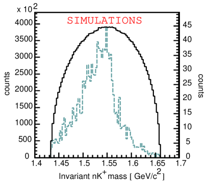
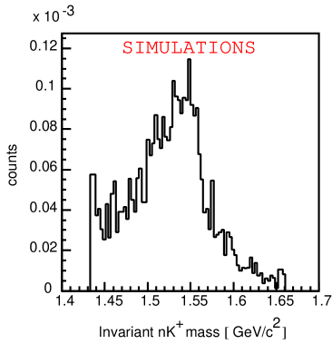
Figure 6.1: (left) Phase space distribution of the invariant mass of the $nK^{+}$ system of the $pp~{}\to~{}nK^{+}\Sigma^{+}$ reaction (solid line) and its convolution with the COSY–11 acceptance (dashed line). (right) The acceptance of the COSY–11 detection setup for the $pp~{}\to~{}nK^{+}\Sigma^{+}$ reaction [21].

The ratio of the obtained invariant mass distributions results in the differential acceptance of COSY–11 facility for detecting the $pp~{}\to~{}nK^{+}\Sigma^{+}$ reaction as shown in figure 6.1(right).

The total acceptance of COSY–11 detection system for the $pp~{}\to~{}nK^{+}\Sigma^{+}$ reaction measured at the beam momentum of 3.257 GeV/c is equal to $10^{-4}$ [20].

Additionally, the simulation of the invariant mass distribution of the process $pp~{}\to~{}\Sigma^{+}\Theta^{+}~{}\to~{}nK^{+}\Sigma^{+}$ has been performed, taking into account the width of $\Theta^{+}$ equal to 5 MeV [24]. The results of the Monte–Carlo calculation are shown in figure 6.2(left).

The expected signal from the $pp~{}\to~{}\Sigma^{+}\Theta^{+}~{}\to~{}n~{}K^{+}\Sigma{+}$ reaction together with the background originating from the direct $pp~{}\to nK^{+}\Sigma^{+}$ reaction is presented in figure 6.2(right).
Here it is assumed arbitrarily that the total cross section for the $pp~{}\to~{}\Sigma^{+}\Theta^{+}$ reaction is ten times smaller than the one for $pp~{}\to~{}nK^{+}\Sigma^{+}$. If the performed appraisals are realistic, one should observed a clear signal in the experiment originating in the $\Theta^{+}$ production as it is noticeable in the right panel of figure 6.2.

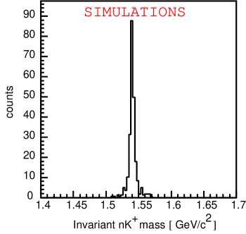
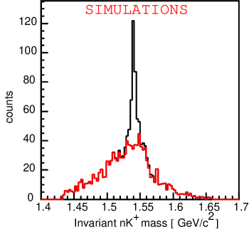
Figure 6.2: (left) Invariant mass distribution of the $nK^{+}$ system for the $pp~{}\to~{}\Sigma^{+}\Theta^{+}~{}\to~{}nK^{+}\Sigma^{+}$ reaction. (right) The expected full invariant mass distribution of the $nK^{+}$ system [21].

A. Kinematics of the $dp~{}\to~{}ppn_{sp}$ reaction

The quasi–free reaction $dp~{}\to~{}ppn_{sp}$ has been used to determine (i) the relative timing between modules, (ii) the general time offset of the neutron detector, and (iii) to establish the momentum resolution of this detector. Due to the Fermi motion of the nucleons bound in the deuteron the simulation of the quasi–free reaction proceeds in following steps :
The components of the Fermi momentum of a nucleon in Cartesian coordinate system are equal to:

$$p_{fx}=p_{F}\cdot\sin\theta\cos\phi$$

$$p_{fy}=p_{F}\cdot\sin\theta\sin\phi$$

$$p_{fz}=p_{F}\cdot\cos\theta$$

As a first step the value of p_F (absolute Fermi momentum) is generated according to the momentum distribution of nucleon inside the deuteron derived from the PARIS potential model [18, 25]. Next the azimuthal angle $\phi$ and cosine of polar angle $\Theta$ ($\cos\Theta$) which define the momentum direction, are generated assuming an uniform distribution. Further the nucleon Fermi momentum inside the deuteron is related to the nucleon momentum in laboratory frame by Lorentz transformation [26]:

$$\vec{p_{f}}^{lab}=\vec{p}_{f}+\vec{\beta}_{d}\gamma(\gamma/(\gamma+1)\vec{\beta}_{d}\cdot\vec{p}_{f}+E_{f})$$

$$E_{f}^{lab}=\gamma(E_{f}+\vec{\beta}_{d}\cdot\vec{p}_{f})$$

where $\beta_{d}$ is the velocity of the deuteron in the laboratory frame and $\gamma$ is equal to:

$$\gamma=1/\sqrt{1-\beta_{d}^{2}}$$

After the momenta of the nucleons inside the deuteron are converted into the LAB system, the proton from the deuteron scatters elastically on a proton target, whereas the neutron does not take part in the reaction, but with momentum possessed at the time of the reaction remains untouched. In order to simulate the proton–proton elastic scattering now we calculate the proton momentum in the proton–proton system using the transformation equation:

$$|\vec{p}_{cm}|=\sqrt{(M^{2}-4m_{p}^{2})/4}$$

where M is the total mass of the colliding protons:

$$M=\sqrt{(\sqrt{\vec{p_{f}}^{{lab}^{2}}+m_{p}^{2}}+m_{p})^{2}-\vec{p_{f}}^{{lab}^{2}}}$$

Once more $\cos\Theta^{cm}$ and $\phi^{cm}$, which define the momentum direction of protons after the scattering in the proton–proton system are generated assuming an uniform distribution. Thus, the components of the proton momentun after scattering are equal to:

$$p_{x}^{cm^{\prime}}=|\vec{p^{cm}}|\sin\theta^{cm}\cos\phi^{cm}$$

$$p_{y}^{cm^{\prime}}=|\vec{p}^{cm}|\sin\theta^{cm}\sin\phi^{cm}$$

$$p_{z}^{cm^{\prime}}=|\vec{p}^{cm}|\cos\theta^{cm}$$

As a last step the proton momentum after scattering in the proton–proton system is related with momentum in laboratory frame by Lorentz transformation:

$$\vec{p^{lab^{\prime}}}=\vec{p^{cm^{\prime}}}+\vec{\beta^{cm}}\gamma^{cm}(\gamma^{cm}/(\gamma^{cm}+1)\vec{\beta^{cm}}\cdot\vec{p^{cm^{\prime}}}+E^{cm^{\prime}}),$$

where

$$\vec{\beta^{cm}}={{\vec{p^{lab}_{f}}}\over{\sqrt{{\vec{p^{lab}_{f}}}^{2}+m^{2}_{p}}+m_{p}}},$$

and

$$\gamma^{cm}={{\sqrt{{\vec{p^{lab}_{f}}}^{2}+m^{2}_{p}}+m_{p}}\over M}.$$

B. Resolution of the measurement of the neutron momentum

The momentum resolution of the neutron detector is a crucial factor in the neutron momentum determination and as shown in figure 6.3 it strongly depends on the momentum of the neutron.

Figure 6.3: Fractional momentum resolution of the neutron detector as a function of neutron momentum.

The momentum of the neutron is calculated from the time–of–flight between the target and the neutron detector and can be expressed as:

$$p=m\cdot{l\over{t^{N}}}\cdot{1\over{\sqrt{1-({l\over{t^{N}}})^{2}}}},$$

where $m$ denotes mass of the particle, $l$ stands for the distance between the target and the neutron detector and $t^{N}$ is the time–of–flight of the particle. A fractional momentum resolution is given by the equation:

$${{\sigma p}\over p}={{{{dp}\over{dt}}\cdot\sigma_{t}}\over p},$$

where $\sigma_{t}$ accounts for both the time resolution of the neutron and S1 detectors and can be written as:

$$\sigma_{t}=\sqrt{\sigma_{n}^{2}+\sigma_{S1}^{2}}$$

The result presented in figure 6.3 was obtained assuming that $\sigma_{n}$ = 0.4 ns, $\sigma_{S1}$ = 0.25 ns, and $l$ = 7 m.

C. Dalitz plot distribution for the $dp\gamma$ system at $\sqrt{s}$ = 3.37 GeV

As a first step for establishing of the double differential acceptance of the COSY–11 facility for the measurement of the $dp~{}\to~{}dp\gamma$ reaction a Dalitz plot distribution for the $dp~{}\to~{}dp\gamma$ reaction was calculated. Figure 6.4 presents the result of calculations assuming that the phase space volume is homogeneously populated. Modifications of this distribution due to the COSY–11 detection setup acceptance remain to be determined.

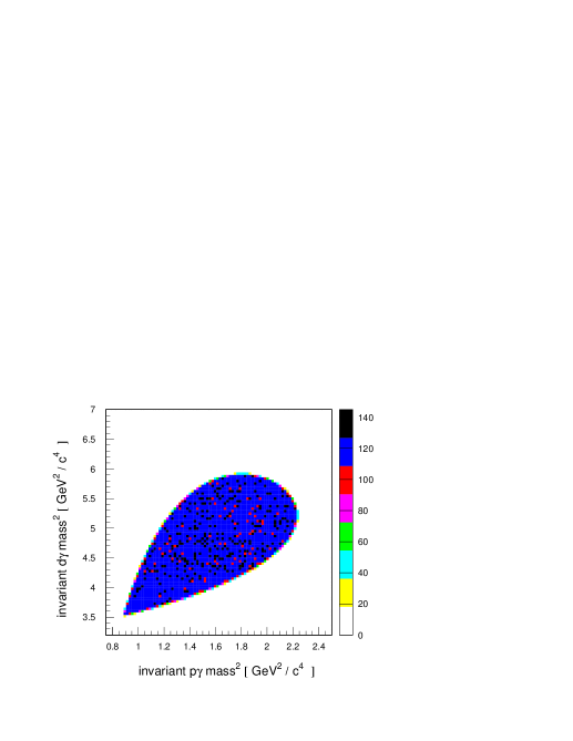
Figure 6.4: Dalitz plot distribution as generated for the $dp~{}\to~{}dp\gamma$ reaction.

Squared of the invariant masses of the $p\gamma$ and $d\gamma$ system can be calculated according to the below equations:

$$S_{p\gamma}={(E_{p}+E_{\gamma})}^{2}-{(\vec{p_{p}}+\vec{p_{\gamma}})}^{2}$$

$$S_{d\gamma}={(E_{d}+E_{\gamma})}^{2}-{(\vec{p_{d}}+\vec{p_{\gamma}})}^{2}$$

It is interesting to note that minimum values for the S_pγ and S_dγ are equal to:

$$S_{p\gamma}^{min}=M_{p}^{2}$$

$$S_{d\gamma}^{min}=M_{d}^{2}$$

References

- [1] N. A. Khokholov et al., Phys. Rev. C 68 054002 (2003).
- [2] M. D. Cozma et al., Phys. Rev. C 68 044003 (2003).
- [3] R. Bilger et al., Phys. Lett B 429 195–200 (1998).
- [4] J. Greiff et al., Phys. Rev. C 65 034009 (2002).
- [5] J. Smyrski, COSY Proposal No. 90 (2001).
- [6] C. Piskor–Ignatowicz, P. Moskal, J. Smyrski, ”Study of the d– interaction via reaction.” Ann. Rep. 2003, IKP, FZ–Jülich (2004).
- [7] H. Dombrowski et al., Nucl. Instr. Meth. A 386 228 (1997).
- [8] P. Moskal et al., Prog. Part. Phys. 49 1–90 (2002).
- [9] P. Moskal et al., e-Print Archive: nucl–ex/0311003.
- [10] M. Janusz, Diploma Thesis, Jagellonian University, Cracow (2004).
- [11] P. Moskal et al., Phys. Rev. C 69 025203 (2004).
- [12] V. Baru et al., Phys. Rev. C 67 024002 (2003).
- [13] S. Brauksiepe et al., Nucl. Instr. Meth. A 376 397 (1996).
- [14] R. Maier, Nucl. Instr. Meth. A 390 1–8 ().
- [15] P. Moskal, Ph.D. Thesis, Jagellonian University, Cracow (1998).
- [16] M. Wolke, Ph.D. Thesis, Universität Bonn, Bonn (1998).
- [17] M. Sokołowski et al., ”Track Reconstruction in a System of Drift Chambers.” Ann. Rep. 1990, IKP, FZ–Jülich, Jül–4052 219 (1991).
- [18] R. Czyżykiewicz, Diploma Thesis, Jagellonian University, Cracow (2002).
- [19] T. Blaich et al., Nucl. Instr. Meth. A 314 136–154 (1992).
-
[20]
J.Przerwa, P. Moskal, ”Study of the Bremmstrahlung radiation in the quasi-free
reaction.”
poster presented at Spring Conference of the German Physical Society (DPG), Cologne, March 2004.
Verhandlungen der DPG (VI) 39, HK 11.12 (2004);
P. Moskal, J. Przerwa, ”Study of the nucleon-nucleon bremsstrahlung radiation at COSY–11” Ann. Rep. 2003, IKP, FZ–Jülich, (2004),
avaiable at: http://ikpe1101.ikp.kfa-juelich.de. -
[21]
J. Przerwa, R. Czyżykiewicz, P. Moskal, C. Piskor-Ignatowicz,
”Searching for the pentaquark at COSY–11”
Ann. Rep. 2003, IKP, FZ–Jülich, (2004);
J. Przerwa, R. Czyżykiewicz, P. Moskal, ”Online analysis of the reaction at COSY–11.” Ann. Rep. 2003, IKP, FZ–Jülich, (2004),
avaiable at: http://ikpe1101.ikp.kfa-juelich.de. - [22] T. Rożek, P. Moskal, ”Time calibration of the COSY–11 neutron detector.” Ann. Rep. 2002, IKP, FZ–Jülich, Jül–4052 (2003).
- [23] T. Rożek — private communication.
- [24] M. Poliakov, talk presented at CANU meeting, Bad Honnef (2003).
- [25] M. Lacombe et al., Phys. Lett. 101 B 139 (1981).
- [26] E. Byckling, K. Kajantie — ”Particle Kinematics”, John Wiley Sons Ltd. (1973).