BES RESULTS ON $J/\psi$ DECAYS AND
CHARMONIUM TRANSITIONS

Abstract

Results are reported based on samples of 58 million $J/\psi$ and 14 million $\psi(2S)$ decays obtained by the BESII experiment. Improved branching fraction measurements are determined, including branching fractions for $J/\psi\to\pi^{+}\pi^{-}\pi^{0}$, $\psi(2S)\rightarrow\pi^{0}J/\psi$, $\eta J/\psi$, $\pi^{0}\pi^{0}J/\psi$, anything $J/\psi$, and $\psi(2S)\rightarrow\gamma\chi_{c1},\gamma\chi_{c2}\rightarrow\gamma\gamma J/\psi$. The decay $J/\psi\to\omega\pi^{+}\pi^{-}$ is studied. At low $\pi\pi$ mass, a large, broad peak due to the $\sigma$ is observed, and its pole position is determined. Results are presented on $\psi(2S)$ and $J/\psi$ hadronic decays to $K^{0}_{S}pK^{-}\bar{n}$ and $K^{0}_{S}\bar{p}K^{+}n$ final states. No significant $\Theta(1540)$ signal, the pentaquark candidate, is observed, and upper limits are set. An enhancement near the $m_{p}+M_{\Lambda}$ mass threshold is observed in the $p\bar{\Lambda}$ invariant mass spectrum from $J/\psi\rightarrow pK^{-}\bar{\Lambda}+c.c.$ decays. It can be fit with an S-wave Breit-Wigner resonance with a mass $m=2075\pm 12\>({\rm stat})\pm 5\>({\rm syst})$ MeV and a width of $\Gamma=90\pm 35\>({\rm stat})\pm 9\>({\rm syst})$ MeV.

Received (20 July 2004)

1 Introduction

The Beijing Spectrometer (BES) is a general purpose solenoidal detector at the Beijing Electron Positron Collider (BEPC). BEPC operates in the center of mass energy range from 2 to 5 GeV with a luminosity at the $J/\psi$ energy of approximately $5\times 10^{30}$ cm^-2s^-1. BES (BESI) is described in detail in Ref. bes1, and the upgraded BES detector (BESII) is described in Ref. bes2.

2 $B(J/\psi\rightarrow\pi^{+}\pi^{-}\pi^{0}$)

The largest $J/\psi$ decay involving hadronic resonances is $J/\psi\rightarrow\rho(770)\pi$. Its branching fraction has been reported by many experimental groups [3] assuming all $\pi^{+}\pi^{-}\pi^{0}$ final states come from $\rho(770)\pi$. The precision of these measurements varies from $13\%$ to 25%. Here, we present two independent measurements of this branching fraction using $J/\psi$ and $\psi(2S)$ decays.

2.1 Absolute measurement of $J/\psi\rightarrow\pi^{+}\pi^{-}\pi^{0}$ decays

Events with two oppositely charged tracks and at least two good photons are selected. A 5-constraint (5C) kinematic fit is made under the $\pi^{+}\pi^{-}\gamma\gamma$ hypothesis with the invariant mass of the two photons being constrained to the $\pi^{0}$ mass, and the fit $\chi^{2}_{\pi^{+}\pi^{-}\pi^{0}}$ is required to be less than 15. After these requirements, 219691 $\pi^{+}\pi^{-}\pi^{0}$ candidates are selected. The branching fraction is $B(J/\psi\rightarrow\pi^{+}\pi^{-}\pi^{0})=(21.84\pm 0.05\pm 2.01)\times 10^{-3}$, where the first error is statistical and the second systematic.

The Dalitz plot of $m_{\pi^{+}\pi^{0}}$ versus $m_{\pi^{-}\pi^{0}}$ is shown in Fig. 1. Three bands are clearly visible in the plot, corresponding to $J/\psi\to\rho\pi$; $J/\psi\rightarrow\pi^{+}\pi^{-}\pi^{0}$ is strongly dominated by $\rho\pi$.

figure=dalitz.eps,height=4.5cm

Figure 1: The Dalitz plot for $J/\psi\to\pi^{+}\pi^{-}\pi^{0}$.

2.2 Relative measurement of $J/\psi\rightarrow\pi^{+}\pi^{-}\pi^{0}$

The relative measurement is based on a sample of 14 million $\psi(2S)$ events. The $\psi(2S)$ is a copious source of $J/\psi$ decays: the branching fraction of $\psi(2S)\rightarrow\pi^{+}\pi^{-}J/\psi$ is the largest single $\psi(2S)$ decay channel. Therefore, we can determine the branching fraction of $J/\psi\rightarrow\pi^{+}\pi^{-}\pi^{0}$ from a comparison of the following two processes:

$$\psi(2S)\rightarrow\pi^{+}\pi^{-} J/\psi$$

$$\hookrightarrow \pi^{+}\pi^{-}\pi^{0}~{}~{}~{}~{}~{}~{}~{}~{}~{}~{}~{}~{}~{}~{}~{}~{}(I)$$

$${\rm and} \hookrightarrow \mu^{+}\mu^{-}~{}~{}~{}~{}~{}~{}~{}~{}~{}~{}~{}~{}~{}~{}~{}~{}~{}(II)$$

Using the relative measurement, many systematic errors mostly cancel. Therefore, the precision of the branching fraction $J/\psi\rightarrow\pi^{+}\pi^{-}\pi^{0}$ from the relative measurement is comparable with that of the direct $J/\psi$ decay, although the size of $\psi(2S)$ sample is smaller.

For process I, a 5C kinematic fit is performed for each candidate event, and the event probability given by the fit must be greater than 0.01. A 4C kinematic fit is performed for $\psi(2S)\rightarrow\pi^{+}\pi^{-}\mu^{+}\mu^{-}$ candidate events, and the probability given by the fit must be greater than 0.01. The branching fraction is $B(J/\psi\rightarrow\pi^{+}\pi^{-}\pi^{0})=(20.91\pm 0.21\pm 1.16)\times 10^{-3}.$

The results of the two measurements are in good agreement. Their weighted mean is

$$B(J/\psi\rightarrow\pi^{+}\pi^{-}\pi^{0})=(2.10\pm 0.12)\%.$$

The result obtained is higher than those of previous measurements and has better precision. For more detail, see Ref. 3pi.

3 $J/\psi\rightarrow\omega\pi^{+}\pi^{-}$

There has been evidence for a low mass pole in the early DM2 [5] and BESI [6] data on $J/\psi\to\omega\pi^{+}\pi^{-}$. Here results on $J/\psi\to\omega\pi^{+}\pi^{-}$ from $5.8\times 10^{7}J/\psi$ events collected with the BESII detector are presented.

The $\omega$ is observed in its $\pi^{+}\pi^{-}\pi^{0}$ decay mode. Events are required to have four good charged tracks with total charge zero and more than one good photon. The TOF and $dE/dx$ information are used to identify pions; they largely reject kaons from background reactions such as $K^{+}K^{-}\pi^{+}\pi^{-}\pi^{0}$. Events with a $2\gamma$ invariant mass $|M_{\gamma\gamma}-M_{\pi^{0}}|<40$ MeV/$c^{2}$ are fitted with a 5C kinematic fit to $\pi^{+}\pi^{-}\pi^{+}\pi^{-}\pi^{0}$ with the two photons being constrained to the $\pi^{0}$ mass. Events with $\chi^{2}_{5C}<40$ are selected. The resulting $\pi^{+}\pi^{-}\pi^{0}$ mass distribution for is shown in Fig. 2(a). The $\omega$ signal is selected by requiring $|M_{\pi^{+}\pi^{-}\pi^{0}}-M_{\omega}|\leq 40$ MeV/$c^{2}$.

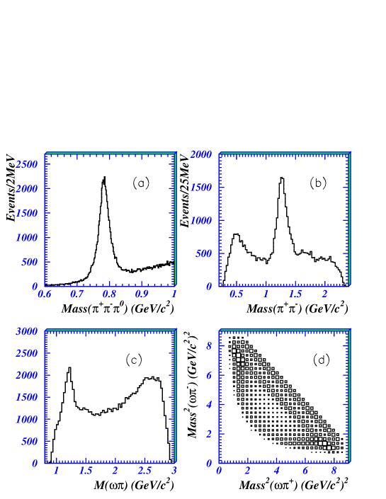
Figure 2: $J/\psi\to\omega\pi^{+}\pi^{-}$ (a.) Distribution of $\pi^{+}\pi^{-}\pi^{0}$ mass. (b.) Distribution of the $\pi^{+}\pi^{-}$ invariant mass recoiling against the $\omega$. (c.) Distribution of $\omega\pi$ invariant mass. (d.) Dalitz plot.

Fig. 2(b) shows the $\pi^{+}\pi^{-}$ invariant mass spectrum which recoils against the $\omega$, and Fig. 2(c) shows the $\omega\pi$ invariant mass. The Dalitz plot of this channel is shown in Fig. 2(d). There is a large $f_{2}(1270)$ peak in Fig. 2(b) and a strong $b_{1}(1235)$ peak in Fig. 2(c). At low $\pi\pi$ masses in Fig. 2(b), a broad enhancement which is due to the $\sigma$ pole is clearly seen. This peak is evident as a strong band along the upper right-hand edge of the Dalitz plot in Fig. 2(d).

Partial wave analyses (PWA) are performed on this channel using two methods. In the first method, the whole mass region of $M_{\pi^{+}\pi^{-}}$ which recoils against the $\omega$ is analyzed, the $\omega$ decay information is used, and the background is subtracted by sideband estimation. For the second method, the region $M_{\pi^{+}\pi^{-}}<1.5$ GeV is analyzed, and the background is fitted by $5\pi$ phase space. In both methods, different parameterizations of the $\sigma$ pole are also studied.

The mass and width of the $\sigma$ are different when using different $\sigma$ parameterizations. However, the pole position of the $\sigma$ is stable; different analysis methods and different parameterizations of the $\sigma$ amplitude give consistent results for the $\sigma$ pole. From a simple mean of the six analyses, the pole position of the $\sigma$ is determined to be $(541\pm 39$ - $i$ $(252\pm 42))$ MeV. Here, the errors cover the statistical and systematic errors in the six analyses, as well as the error in the extrapolation to the pole. The systematic errors dominate. More detail may be found in Ref. sigma.

4 $\psi(2S)\rightarrow\gamma\gamma J/\psi$ and $\psi(2S)\rightarrow XJ/\psi$

Experimental results for the processes $\psi(2S)\rightarrow\pi^{0}J/\psi$, $\eta J/\psi$, and $\gamma\chi_{c1,2}$ are few and were mainly taken in the 1970s and 80s. [3] Here, we report on the analysis of $\psi(2S)\rightarrow\pi^{0}J/\psi$, $\eta J/\psi$, and $\gamma\chi_{c1,2}$ decays based on a sample of $14.0\times 10^{6}$ $\psi(2S)$ events collected with the BESII detector. Events with two charged tracks identified as an electron pair or muon pair and two or three photon candidates are selected. A five constraint (5C) kinematic fit to the hypothesis $\psi(2S)\rightarrow\gamma\gamma l^{+}l^{-}$ with the invariant mass of the lepton pair constrained to $J/\psi$ mass is performed, and the fit probability is required to be greater than 0.01.

Fig. 3 shows, after a cut to remove the huge background from $\psi(2S)\rightarrow\gamma\chi_{c1,c2}$ under the $\psi(2S)\rightarrow\pi^{0}J/\psi$ signal, the distribution of invariant mass, $M_{\gamma\gamma}$. A Breit Wigner with a double Gaussian mass resolution function to describe the $\pi^{0}$ resonance plus a background polynomial is fitted to the data. Similar analyses are made for the other channels.

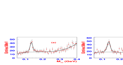
Figure 3: Two photon invariant mass distribution for candidate $\psi(2S)\rightarrow\pi^{0}J/\psi$ events for (a) $\gamma\gamma e^{+}e^{-}$ and (b) $\gamma\gamma\mu^{+}\mu^{-}$.

Results from $\psi(2S)\rightarrow\gamma\gamma J/\psi$ Channel $\pi^{0}J/\psi$ $\eta J/\psi$ Final state $\gamma\gamma e^{+}e^{-}$ $\gamma\gamma\mu^{+}\mu^{-}$ $\gamma\gamma e^{+}e^{-}$ $\gamma\gamma\mu^{+}\mu^{-}$ B (%) $0.139\pm 0.020\pm 0.013$ $0.147\pm 0.019\pm 0.013$ $2.91\pm 0.12\pm 0.21$ $3.06\pm 0.14\pm 0.25$ Combined (%) $0.143\pm 0.014\pm 0.013$ $2.98\pm 0.09\pm 0.23$ PDG (%)[3] $0.096\pm 0.021$ $3.16\pm 0.22$ Channel $\gamma\chi_{c1}$ $\gamma\chi_{c2}$ Final state $\gamma\gamma e^{+}e^{-}$ $\gamma\gamma\mu^{+}\mu^{-}$ $\gamma\gamma e^{+}e^{-}$ $\gamma\gamma\mu^{+}\mu^{-}$ B (%) $8.73\pm 0.21\pm 1.00$ $9.11\pm 0.24\pm 1.12$ $7.90\pm 0.26\pm 0.88$ $8.12\pm 0.23\pm 0.99$ Combined (%) $8.90\pm 0.16\pm 1.05$ $8.02\pm 0.17\pm 0.94$ PDG (%)[3] $8.4\pm 0.6$ $6.4\pm 0.6$

Using the fitting results and the efficiencies and correction factors for each channel, the branching fractions listed in Table 4 are determined. The BES $B(\psi(2S)\rightarrow\pi^{0}J/\psi)$ measurement has improved precision by more than a factor of two compared with other experiments, and the $\psi(2S)\rightarrow\eta J/\psi$ branching fraction is the most accurate single measurement. More details on this analysis may be found in Ref. ggJ.

In another analysis, based on a sample of approximately $4\times 10^{6}$ $\psi(2S)$ events obtained with the BESI detector, [9] a different technique is used for measuring branching fractions for the inclusive decay $\psi(2S)\rightarrow{\rm anything}J/\psi$, and the exclusive processes for the cases where $X=\eta$ and $X=\pi\pi$, as well as the cascade processes $\psi(2S)\rightarrow\gamma\chi_{c0/1/2}$, $\chi_{c0/1/2}\rightarrow\gamma J/\psi$. Inclusive $\mu^{+}\mu^{-}$ pairs are reconstructed, and the number of $\psi(2S)\rightarrow J/\psi X$ events is determined from the $J/\psi\rightarrow\mu^{+}\mu^{-}$ peak in the $\mu^{+}\mu^{-}$ invariant mass distribution. The exclusive branching fractions are determined from fits to the distribution of masses recoiling from the $J/\psi$ with Monte-Carlo determined distributions for each individual channel.

The mass recoiling against the $J/\psi$ candidates, $m_{X}$ is determined from energy and momentum conservation. To determine the number of exclusive decays and separate $\psi(2S)\rightarrow J/\psi\pi^{0}\pi^{0}$ and $\psi(2S)\rightarrow J/\psi\pi^{+}\pi^{-}$ events, $m_{X}$ histograms for events with and without additional charged tracks, shown in Figs. 5 and 5, are fit simultaneously. To reduce background and improve the quality of the track momentum measurements, events used for this part of the analysis are required to have a kinematic fit $\chi^{2}<7$. The channels of interest are normalized to the observed number of $\pi^{+}\pi^{-}J/\psi$ events; ratios of the studied branching fractions to that for $B(\psi(2S)\rightarrow\pi^{+}\pi^{-}J/\psi)$ are reported. This has that advantage that many of the systematic errors largely cancel.

Figure 4: Fit of the $m_{X}$ distribution events with no additional charged tracks. Shown are the data (points with error bars), the component histograms, and the final fit. For the components, the large, long-dash histogram is $\psi(2S)\rightarrow J/\psi\pi\pi$, the narrow, dash-dot histogram is $\psi(2S)\rightarrow J/\psi\eta$, the broad, short-dashed histogram is $\psi(2S)\rightarrow\gamma\chi_{c1},\chi_{c1}\rightarrow\gamma J/\psi$, the broad, hatched histogram is $\psi(2S)\rightarrow\gamma\chi_{c2},\chi_{c2}\rightarrow\gamma J/\psi$, and the lowest cross-hatched histogram is the combined $e^{+}e^{-}\rightarrow\gamma\mu^{+}\mu^{-}$ and $e^{+}e^{-}\rightarrow\psi(2S),\psi(2S)\rightarrow(\gamma)\mu^{+}\mu^{-}$ background. The final fit is the solid histogram.

Figure 5: Fit of the $m_{X}$ distribution for events with any number of additional charged tracks. Shown are the data (points with error bars), the component histograms, and the final fit (solid histogram). The dashed histogram is $\psi(2S)\rightarrow J/\psi\pi^{+}\pi^{-}$, and the hatched histogram is $\psi(2S)\rightarrow J/\psi\eta$. There is very little evidence for $\psi(2S)\rightarrow\gamma\chi_{c1/2},\chi_{c1/2}\rightarrow\gamma J/\psi$. This distribution is composed predominantly of $\psi(2S)\rightarrow J/\psi\pi^{+}\pi^{-}$.

Final branching ratios and branching fractions. PDG04-exp results are single measurements or averages of measurements, while PDG04-fit are results of their global fit to many experimental measurements. The BES results in the second half of the table are calculated using the PDG04 value of $B_{\pi\pi}=B(\psi(2S)\rightarrow J/\psi\pi^{+}\pi^{-})=(31.7\pm 1.1)\%$. Case This result PDG04-exp PDG04-fit $B(J/\psi\>({\rm anything})/B_{\pi\pi}$ $1.867\pm 0.026\pm 0.055$ $2.016\pm 0.150$ $1.821\pm 0.036$ $B(J/\psi\pi^{0}\pi^{0})/B_{\pi\pi}$ $0.570\pm 0.009\pm 0.026$ - $0.59\pm 0.05$ $B(J/\psi\eta)/B_{\pi\pi}$ $0.098\pm 0.005\pm 0.010$ $0.091\pm 0.021$ $0.100\pm 0.008$ $B(\gamma\chi_{c1})B(\chi_{c1}\rightarrow\gamma J/\psi)/B_{\pi\pi}$ $0.126\pm 0.003\pm 0.038$ $0.085\pm 0.021$ $0.084\pm 0.006$ $B(\gamma\chi_{c2})B(\chi_{c2}\rightarrow\gamma J/\psi)/B_{\pi\pi}$ $0.060\pm 0.000\pm 0.028$ $0.039\pm 0.012$ $0.041\pm 0.003$ $B(J/\psi\>({\rm anything})$ (%) $59.2\pm 0.8\pm 2.7$ $55\pm 7$ $57.6\pm 2.0$ $B(J/\psi\pi^{0}\pi^{0})$ (%) $18.1\pm 0.3\pm 1.0$ – $18.8\pm 1.2$ $B(J/\psi\eta)$ (%) $3.11\pm 0.17\pm 0.31$ $2.9\pm 0.5$ $3.16\pm 0.22$ $B(\gamma\chi_{c1})B(\chi_{c1}\rightarrow\gamma J/\psi)$ (%) $4.0\pm 0.1\pm 1.2$ $2.66\pm 0.16$ $2.67\pm 0.15$ $B(\gamma\chi_{c2})B(\chi_{c2}\rightarrow\gamma J/\psi)$ (%) $1.91\pm 0.01\pm 0.86$ $1.20\pm 0.13$ $1.30\pm 0.08$

The final branching fraction ratios and branching fractions are shown in Table 4, along with the PDG experimental averages and global fit results. The results for $B(J/\psi\>{\rm anything})/B(\psi(2S)\rightarrow\pi^{+}\pi^{-}J/\psi)$ and $B(\eta J/\psi)/B(\psi(2S)\rightarrow\pi^{+}\pi^{-}J/\psi)$ have smaller errors than the previous results. The agreement for both the ratios of branching fractions and the calculated branching fractions using the PDG result for $\psi(2S)\rightarrow B(\pi^{+}\pi^{-}J/\psi)$ with the PDG fit results is good, and the determination of $B(\eta J/\psi)$ agrees well with the determination from $\psi(2S)\rightarrow\gamma\gamma J/\psi$ decays above. More details on this analysis may be found in Ref. Xjpsi.

5 Pentaquark Search

The pentaquark,[11] the main topic of the opening session of this conference, has generated much excitement. BES has searched for the pentaquark state $\Theta(1540)$ in $\psi(2S)$ and $J/\psi$ decays to $K^{0}_{S}pK^{-}\bar{n}$ and $K^{0}_{S}\bar{p}K^{+}n$ final states using samples of 14 million $\psi(2S)$ and 58 million $J/\psi$ events taken with BES II. These processes could contain $\Theta$ decays to $K^{0}_{S}p,~{}K^{+}n~{}(uudd\bar{s})$ and $\bar{\Theta}$ decays to $K^{0}_{S}\bar{p},~{}K^{-}n~{}(\bar{u}\bar{u}\bar{d}\bar{d}s)$.

The anti-neutron and neutron are not detected. The $K^{0}_{S}$ meson in the event is identified through the decay $K^{0}_{S}\to\pi^{+}\pi^{-}$. Candidate events are kinematically fitted under the assumption of a missing $\bar{n}(n)$ to obtain better mass resolution and to suppress the backgrounds. Events with missing mass close to the $\bar{n}(n)$’s mass are selected. We use the same criteria and treatment for both $\psi(2S)$ and $J/\psi$ data.

Figure 6: Scatter plot of $K^{-}n~{}(K^{0}_{S}\bar{p})$ versus $K^{0}_{S}p~{}(K^{+}n)$ for $\psi(2S)\to K^{0}_{S}pK^{-}\bar{n}$ + $K^{0}_{S}\bar{p}K^{+}n$ modes.

The scatter plot of $K^{-}n~{}(K^{0}_{S}\bar{p})$ versus $K^{0}_{S}p~{}(K^{+}n)$ for $\psi(2S)\to K^{0}_{S}pK^{-}\bar{n}$ + $K^{0}_{S}\bar{p}K^{+}n$ modes is shown in Fig. 6. Zero events fall within the signal region, shown as a square centered at $(1.540,1.540)$ GeV/c², and we set an upper limit at the 90% confidence level (C.L.) on the branching ratio:

$${\cal B}(\psi(2S)\to\Theta\bar{\Theta}\to K^{0}_{S}pK^{-}\bar{n}+K^{0}_{S}\bar{p}K^{+}n)<0.84\times 10^{-5}.$$

Another possibility is that the $\psi(2S)$ decays to only one $\Theta$ or $\bar{\Theta}$ state. To determine the number of $\Theta(1540)$ events from single $\Theta$ or $\bar{\Theta}$ production, we count the number of events within regions of 1.52 - 1.56 GeV$/c^{2}$ in the projections of Fig. 6 and set upper limits, shown in Table 5.

Summary of upper limits. Decay mode   $\psi(2S)$ $J/\psi$ $\to\Theta\bar{\Theta}\to K^{0}_{S}pK^{-}\bar{n}x+K^{0}_{S}\bar{p}K^{+}n$ $0.88\times 10^{-5}$ $1.1\times 10^{-5}$ $\to\Theta K^{-}\bar{n}\to K^{0}_{S}pK^{-}\bar{n}$ $1.0\times 10^{-5}$ $2.1\times 10^{-5}$ $\to\bar{\Theta}K^{+}n\to K^{0}_{S}\bar{p}K^{+}n$ $2.6\times 10^{-5}$ $5.6\times 10^{-5}$ $\to K^{0}_{S}p\bar{\Theta}\to K^{0}_{S}pK^{-}\bar{n}$ $0.60\times 10^{-5}$ $1.1\times 10^{-5}$ $\to K^{0}_{S}\bar{p}\Theta\to K^{0}_{S}\bar{p}K^{+}n$ $0.70\times 10^{-5}$ $1.6\times 10^{-5}$

For the decays of $J/\psi\to K^{0}_{S}pK^{-}\bar{n}$ and $K^{0}_{S}\bar{p}K^{+}n$, we use the same criteria and analysis method as those used for the $\psi(2S)$ data to study possible $\Theta(1540)$ production. There is no significant $\Theta(1540)$ signal, and we determine upper limits on the branching fractions at the 90% C.L., shown in Table 5. Full details may be found in Ref. penta.

6 Enhancement in the $p\bar{\Lambda}$ invariant mass spectrum in $J/\psi\rightarrow pK^{-}\bar{\Lambda}$ and in $\psi(2S)\rightarrow pK^{-}\bar{\Lambda}$ decays

An anomalous enhancement near the mass threshold in the $p\bar{p}$ invariant mass spectrum was observed by the BES II experiment in $J/\psi\rightarrow\gamma p\bar{p}$ decays. [13] This enhancement can be fitted with an S-wave Breit-Wigner resonance function with a mass around 1860 MeV and a width $\Gamma<30$ MeV, and has been interpreted as a possible baryonium state. [14] Similar $p\bar{p}$ mass-threshold enhancements have been observed in the decays $B^{+}\rightarrow K^{+}p\bar{p}$ and $\bar{B}^{0}\rightarrow D^{0}p\bar{p}$ by the Belle Collaboration.  [15, 17] It is, therefore, of special interest to search for possible resonant structures in other baryon-antibaryon final states. The Belle Collaboration recently observed a near-threshold enhancement in the $p\bar{\Lambda}$ mass spectrum from $B\rightarrow p\bar{\Lambda}\pi$ decays. [16] We report the observation of an enhancement near threshold in the $p\bar{\Lambda}$ invariant mass spectrum in $J/\psi\rightarrow pK^{-}\bar{\Lambda}$ and in $\psi(2S)\rightarrow pK^{-}\bar{\Lambda}$ decays. The results are based on an analysis of $5.8\times 10^{7}$ $J/\psi$ and $1.4\times 10^{7}$ $\psi(2S)$ decays detected in BESII.

The $J/\psi\rightarrow pK^{-}{\bar{\Lambda}}$ candidate events are required to have four good charged tracks with total charge zero. Events are subjected to a four-constraint (4C) kinematic fit with the corresponding mass assignments for each track. For events with ambiguous particle identification, all possible 4C combinations are formed, and the combination with the smallest $\chi^{2}$ is chosen. A sample of $5421$ $J/\psi\rightarrow pK^{-}{\bar{\Lambda}}$ candidates survive the final selection. Monte Carlo studies indicate that the background in the selected event sample is at the $1\sim 2\%$ level.

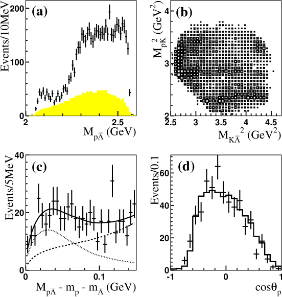
Figure 7: (a) The points with error bars indicate the measured $p\bar{\Lambda}$ mass spectrum; the shaded histogram indicates phase space MC events (arbitrary normalization). (b) The Dalitz plot for the selected event sample. (c) A fit (solid line) to the data. The dotted curve indicates the Breit-Wigner signal and the dashed curve the phase space ‘background.’ (d) The $\cos\theta_{p}$ distribution under the enhancement, the points are data and the histogram is the MC (normalized to data)

The $p\bar{\Lambda}$ invariant mass spectrum for the selected events is shown in Fig. 7(a), where an enhancement is evident near the mass threshold. No corresponding structure is seen in a sample of $J/\psi\rightarrow pK^{-}\bar{\Lambda}$ MC events generated with a uniform phase space distribution. The $pK^{-}\bar{\Lambda}$ Dalitz plot is shown in Fig. 7(b). In addition to bands for the well established $\Lambda^{*}(1520)$ and $\Lambda^{*}(1690)$, there is a significant $N^{*}$ band near the $K^{-}\bar{\Lambda}$ mass threshold, and a $p\bar{\Lambda}$ mass enhancement, isolated from the $\Lambda^{*}$ and $N^{*}$ bands, in the right-upper part of the Dalitz plot.

This enhancement can be fit with an acceptance weighted S-wave Breit-Wigner function, together with a function describing the phase space contribution, as shown in Fig. 7(c). The fit gives a peak mass of $m=2075\pm 12\pm 5$ MeV and a width $\Gamma=90\pm 35\pm 9$ MeV. The significance is about $7\sigma$. A P-wave Breit-Wigner resonance functions can also fit the enhancement. The $\cos\theta_{p}$ distribution, shown in Fig. 7(d), where $\theta_{p}$ is the decay angle of p in the $p\bar{\Lambda}$ CM frame, agrees well with that of a MC sample of $J/\psi\rightarrow KX\rightarrow Kp\bar{\Lambda}$. Since the MC $\cos\theta_{p}$ distribution is generated as a uniform S-wave distribution and the detected MC distribution agrees with data in Fig. 7(d), the observed distribution for the enhancement is consistent with S-wave decays to $p\bar{\Lambda}$.

Evidence of a similar enhancement is observed in $\psi(2S)\rightarrow pK^{-}\bar{\Lambda}$ when the same analysis is performed on the $\psi(2S)$ data sample. More detail can be found in Ref. pklambda.

References

- [1] J. Z. Bai et al., (BES Collab.), Nuc. Inst. Meth. A344, 319 (1994).
- [2] J. Z. Bai et al., (BES Collab.), Nuc. Inst. Meth. A458, 627 (2001).
- [3] S. Eidelman et al., (Particle Data Group), Phys. Lett. B592, 1 (2004).
- [4] J. Z. Bai et al., (BES Collab.), accepted by Phys. Rev. D, hep-ex/0402013.
- [5] J.E. Augustin et al., Nucl. Phys. B320, 1 (1989).
- [6] Ning Wu (BES Collab.), Proceedings of the XXXVIth Rencontres de Moriond, Les Arcs, France, March 17-24, (2001).
- [7] M. Ablikim et al., (BES Collab.), accepted by Phys. Lett. B, hep-ex/0406038.
- [8] M. Ablikim et al., (BES Collab.), accepted by Phys. Rev. D, hep-ex/0403023.
- [9] J.Z. Bai et al., (BES Collab.), Nucl. Inst. Meth. A344, 319 (1994).
- [10] M. Ablikim et al., BES Collab., accepted by Phys. Rev. D, hep-ex/0404020.
- [11] T. Nakano et al. (LEPS Collab.), Phys. Rev. Lett. 91, 012002 (2003).
- [12] M. Ablikim et al., (BES Collab.), accepted by Phys. Rev. D, hep-ex/0402012.
- [13] J.Z. Bai et al., (BES Collab.), Phys. Rev. Lett. 91, 022001 (2003).
- [14] Alakabha Datta, Patrick J. O’Donnell, Phys. Lett. B567, 273 (2003).
- [15] K. Abe et al., (Belle Collab.), Phys. Rev. Lett. 88, 181803 (2002).
- [16] M.Z. Wang et al., (Belle Collab.), Phys. Rev. Lett. 90, 201802 (2003).
- [17] K. Abe et al., (Belle Collab.), Phys. Rev. Lett. 89, 151802 (2002).
- [18] M. Ablikim et al., (BES Collab.), accepted by Phys. Rev. Lett., hep-ex/0405050.