Quark helicity distributions in the nucleon for up, down, and strange quarks from semi–inclusive deep–inelastic scattering

Abstract

Polarized deep–inelastic scattering data on longitudinally polarized hydrogen and deuterium targets have been used to determine double spin asymmetries of cross sections. Inclusive and semi–inclusive asymmetries for the production of positive and negative pions from hydrogen were obtained in a re–analysis of previously published data. Inclusive and semi–inclusive asymmetries for the production of negative and positive pions and kaons were measured on a polarized deuterium target. The separate helicity densities for the up and down quarks and the anti–up, anti–down, and strange sea quarks were computed from these asymmetries in a “leading order” QCD analysis. The polarization of the up–quark is positive and that of the down–quark is negative. All extracted sea quark polarizations are consistent with zero, and the light quark sea helicity densities are flavor symmetric within the experimental uncertainties. First and second moments of the extracted quark helicity densities in the measured range are consistent with fits of inclusive data.

I Introduction

Understanding the internal structure of the nucleon remains a fundamental challenge of contemporary hadron physics. From studies of deep-inelastic lepton-nucleon scattering(DIS), much has been learned about the quark-gluon structure of the nucleon, but a clear picture of the origins of its spin has yet to emerge. The pioneering experiments to explore the spin structure of the nucleon performed at SLAC Alguard et al. (1976); Baum et al. (1983) were measurements of inclusive spin asymmetries, in which only the scattered lepton is observed. Until recently, inclusive measurements have provided most of the current knowledge of nucleon spin structure. The objective of these studies was to determine the fraction of the spin of the nucleon which is carried by the quarks. The nucleon spin can be decomposed conceptually into the angular momentum contributions of its constituents according to the equation

$$\langle s^{N}_{z}\rangle=\frac{1}{2}=\frac{1}{2}{\Delta\Sigma}+{L_{q}}+{J_{g}},$$ (1)

where the three terms give the contributions to the nucleon spin from the quark spins, the quark orbital angular momentum, and the total angular momentum of the gluons, respectively. Early calculations based on relativistic quark models Jaffe and Manohar (1990); Suzuki and Weise (1998) suggested $\Delta\Sigma\approx 2/3$, while more precise experiments on DIS at CERN, performed by the European Muon Collaboration (EMC) Ashman et al. (1988, 1989), led to the conclusion that $\Delta\Sigma\approx 0.1-0.2$.

With these indications of the complexity of the spin structure, it was quickly realized that a simple leading order (LO) analysis that did not include contributions from gluons was incomplete. More recent next-to-leading order (NLO) treatments provide a picture more appropriate to our present understanding of QCD. The focus has been on the polarized structure function $g_{1}(x,Q^{2})$ for the proton, given by Altarelli et al. (1997)

$$\begin{split}g_{1}(x,Q^{2})&=\frac{\langle e^{2}\rangle}{2}[C_{NS}(x,\alpha_{s}(Q^{2}))\otimes\Delta q_{NS}(x,Q^{2})\\ &+C_{S}(x,\alpha_{s}(Q^{2}))\otimes\Delta\Sigma(x,Q^{2})\\ &+2n_{f}C_{g}(x,\alpha_{s}(Q^{2}))\otimes\Delta g(x,Q^{2})],\end{split}$$ (2)

where $\langle e^{2}\rangle=n_{f}^{-1}\Sigma_{i=1}^{n^{f}}e^{2}_{i}$, $e_{i}$ is the electric charge of the quark of flavor $q$, the operator $\otimes$ denotes convolution over $x$, $\Delta q_{NS}$ and $\Delta\Sigma$ are respectively the nonsinglet and singlet quark helicity distributions, and $\Delta g$ is the gluon helicity distribution. Here $x$ is the usual Bjorken scaling variable, $-Q^{2}$ is the squared four–momentum transfer, and $n_{f}$ is the number of active quark flavors. The coefficient functions $C_{NS}$, $C_{S}$, and $C_{g}$ have been computed up to next-to-leading order Mertig and van Neerven (1996); Vogelsang (1996) in $\alpha_{s}$. At NLO they as well as their associated parton distributions depend on the renormalization and factorization schemes. While the physical observables are scheme independent, parton distributions will be strongly scheme dependent, but connected from scheme to scheme by well-defined relationships. In a recent NLO analysis Adeva et al. (1998a) of available data for $g_{1}$, the SMC group presented results for the first moment of $g_{1}$, which is given by

$$\begin{split}\int_{0}^{1}dx\>g_{1}(x,Q^{2})&=\frac{\langle e^{2}\rangle}{2}[C_{NS}(Q^{2},\alpha_{s}(Q^{2})){\Delta}q_{NS}(Q^{2})\\ +&C_{S}(Q^{2},\alpha_{s}(Q^{2}))a_{0}(Q^{2})],\end{split}$$ (3)

where the $Q^{2}$ dependent quantities $C_{NS}$, $C_{S}$, and ${\Delta}q_{NS}$ are the first moments over $x$. In the Adler–Bardeen scheme used by the SMC group the singlet axial charge $a_{0}$ is

$$a_{0}(Q^{2})=\Delta\Sigma-3\frac{\alpha_{s}(Q^{2})}{2\pi}\Delta g(Q^{2}),$$ (4)

where $\Delta\Sigma$ is the first moment of the singlet quark distribution, and $\Delta g(Q^{2})$ the gluonic first moment. The SMC group finds that the analysis of the $Q^{2}$ evolution of the world data base gives $\Delta\Sigma=0.38^{+0.03}_{-0.03}$ (stat)${}^{+0.03}_{-0.02}$(syst)${}^{+0.03}_{-0.05}$(th) and $\Delta g(1{\mathrm{GeV}}^{2})=0.99^{+1.17}_{-0.31}$ (stat)${}^{+0.42}_{-0.22}$(syst)${}^{+1.43}_{-0.45}$(th). The resulting value of the singlet axial charge is $a_{0}=0.23\pm 0.07$(stat)$\pm 0.19$(syst). While this result strongly constrains the total quark spin contribution to the nucleon spin, the limited information it provides on the flavor structure of $\Delta\Sigma$ is critically dependent on the assumptions of $SU(3)$ flavor symmetry in the interpretation of hyperon beta–decay which are made to constrain $\Delta q_{NS}$. A central issue in the analysis of the inclusive data from these experiments is their sensitivity to $SU(3)$ symmetry breaking, and the reliability of estimates of the contributions to the first moments coming from the unmeasured low $x$ region.

With rare exceptions, the experiments listed above have studied inclusive polarized DIS where only the scattered lepton is detected. Their sensitivity is limited to the polarization of the combination of quarks and antiquarks because the scattering cross section depends on the square of the charge of the target parton. The key to further progress is more specific probes of the individual contributions of Eq. (1) to the proton spin. Determination of the polarization of the gluons is clearly of high priority, and a more precise measurement will eliminate a major current ambiguity in the implications of existing inclusive data. A more direct determination of the strange quark polarization will avoid the need for the use of data from hyperon decay and the assumption of $SU(3)$ flavor symmetry. Measurements which are sensitive to quark flavors will allow the separation of quark and antiquark polarizations. The HERMES experiment attempts to achieve these objectives by emphasizing semi-inclusive DIS, in which a $\pi,K,$ or $p$ is observed in coincidence with the scattered lepton. The added dimension of flavor in the final hadron provides a valuable probe of the flavor dependence and other features of parton helicity distributions. With the advanced state of inclusive measurements and the HERMES data with its added dimension in the flavor sector, important issues such as measurements of moments of matrix elements and their accessibility to measurement can be revisited. Indeed, the results reported here, which address the issue of the flavor dependence of quark helicity densities, mark the logical next step in unraveling the spin structure of the proton.

This paper begins with a brief development of the formalism required to describe semi–inclusive DIS. It is followed by a description of the HERMES experiment and the analysis procedures for flavor tagging which produce a comprehensive set of spin asymmetries and a detailed flavor decomposition of the quark helicity densities in the nucleon. The formalism and experiment are described in sections II and III. Sections IV and V detail the analysis procedures and the resulting cross section asymmetries. The extraction of the helicity distributions is explained in section VI, while section VII summarizes an alternative approach to measuring strange quark distributions. Partial first and second moments of the extracted helicity distributions and of their singlet and non–singlet combinations in the measured kinematic range are given in section VIII, where they are also compared to other existing measurements and to results from global QCD fits. The conclusions from these results are discussed in section IX. The formalism used for the QED radiative and detector smearing corrections is presented in some detail in App. A and tables with the numerical results of the present analysis are given in App. B.

II Polarized DIS

II.1 Polarized Inclusive DIS Formalism

The main process studied here is depicted in Fig. 1. An incoming positron or electron emits a spacelike virtual photon, which is absorbed by a quark in the nucleon. The nucleon is broken up, and the struck quark and the target remnant fragment into hadrons in the final state. Only the lepton is detected in inclusive measurements while detection of one or more hadrons in the final state in semi–inclusive measurements adds important information on the scattering process. Contributions from Z⁰ exchange can be neglected at the energy of the present experiment.

The kinematic variables relevant for this process are listed in Tab. 1. The formalism for DIS is developed in many texts on particle physics Halzen and Martin (1984); Roberts (1990); Thomas and Weise (2001). Here, the formalism for polarized DIS is briefly summarized in order to introduce the various measured quantities.

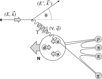
Figure 1: Diagram of the deep-inelastic scattering process. The incoming lepton emits a virtual photon which is absorbed by one of the quarks in the nucleon. In the case depicted, the struck quark fragments into a pion in the final state. In semi–inclusive processes, the scattered lepton and part of the hadronic final state are detected in coincidence.

The inclusive DIS cross–section can be written as follows:

$$\frac{d^{2}\sigma}{dx\,dQ^{2}}\propto\,L_{\mu\nu}\,W^{\mu\nu}\,,$$ (5)

where $L_{\mu\nu}$ is a tensor that describes the emission of the virtual photon by the lepton and other radiative processes; it can be calculated in Quantum Electro Dynamics (QED). The tensor $W^{\mu\nu}$ describes the absorption of the virtual photon by the target; it contains all of the information related to the structure of the target. Symmetry considerations and conservation laws determine the form of $W^{\mu\nu}$ (cf. Roberts (1990); Thomas and Weise (2001)), which for a spin–$1/2$ target and pure electromagnetic interaction reads:

$$\begin{split}\!W_{\mu\nu}&=\left(-g_{\mu\nu}-\frac{q_{\mu}\,q_{\nu}}{Q^{2}}\right)F_{1}\\ +&\left(P_{\mu}+\frac{P\cdot q}{Q^{2}}\,q_{\mu}\right)\left(P_{\nu}+\frac{P\cdot q}{Q^{2}}\,q_{\nu}\right)\frac{F_{2}}{P\cdot q}\\ +&\,i\epsilon_{\mu\nu\alpha\beta}\,q^{\alpha}\frac{M}{P\cdot q}\left[S^{\beta}\,g_{1}+\left(S^{\beta}-\frac{S\cdot q}{P\cdot q}\,P^{\beta}\right)g_{2}\right]\,.\end{split}$$ (6)

Table 1: Kinematic variables in deep inelastic scattering

$k=(E,\vec{k})$, $k^{\prime}=(E^{\prime},\vec{k^{\prime}})$	4–momenta of the initial and final state leptons
$\theta,\;\phi$	Polar and azimuthal angle of the scattered lepton
$P\stackrel{{\scriptstyle\mathrm{lab}}}{{=}}(M,0)$	4–momentum of the initial target nucleon
$q=k-k^{\prime}$	4–momentum of the virtual photon
$Q^{2}\equiv-q^{2}$ $\stackrel{{\scriptstyle\mathrm{lab}}}{{=}}4EE^{\prime}\sin^{2}\frac{\theta}{2}$	Negative squared 4–momentum transfer
$\nu\equiv\frac{P\cdot q}{M}\stackrel{{\scriptstyle\mathrm{lab}}}{{=}}E-E^{\prime}$	Energy of the virtual photon
$x=\frac{Q^{2}}{2\,P\cdot q}=\frac{Q^{2}}{2\,M\nu}$	Bjorken scaling variable
$y\equiv\frac{P\cdot q}{P\cdot k}\stackrel{{\scriptstyle\mathrm{lab}}}{{=}}\frac{\nu}{E}$	Fractional energy of the virtual photon
$W^{2}=(P+q)^{2}$ $=M^{2}+2M\nu-Q^{2}$	Squared invariant mass of the photon–nucleon system
$p=(E_{h},\vec{p})$	4–momentum of a hadron in the final state
$z=\frac{P\cdot p}{P\cdot q}\stackrel{{\scriptstyle\mathrm{lab}}}{{=}}\frac{E_{h}}{\nu}$	Fractional energy of the observed final state hadron
$x_{F}=\frac{p_{CM}^{\|}}{|\vec{q}|}\stackrel{{\scriptstyle\mathrm{lab}}}{{\simeq}}\frac{2\,p_{CM}^{\|}}{W}$	Longitudinal momentum fraction of the hadron

In this expression, $F_{1}$ and $F_{2}$ are unpolarized structure functions, while $g_{1}$ and $g_{2}$ are polarized structure functions that contribute to the cross section only if both the target and the beam are polarized. The usual Minkowski metric is given by $g_{\mu\nu}$, and $\epsilon_{\mu\nu\alpha\beta}$ is the totally anti–symmetric tensor. The four–vector $S$ is the spin of the nucleon, and $q$ and $P$ are defined in Tab. 1. In general, the structure functions depend on $\nu$ and $Q^{2}$. They can also be defined in terms of the dimensionless scaling variables $y$, the fractional energy transfer to the nucleon, and $x$, the Bjorken scaling variable. The latter is equal to the fraction of the nucleon’s light-cone momentum carried by the struck quark.

The structure functions are given in the quark–parton model (QPM) by:

$$F_{1}(x) =\frac{1}{2}\sum_{q}e_{q}^{2}\;(q^{+}(x)+q^{-}(x))=\frac{1}{2}\sum_{q}e_{q}^{2}\;q(x)\,,$$ (7)

$$g_{1}(x) =\frac{1}{2}\sum_{q}e_{q}^{2}\;(q^{+}(x)-q^{-}(x))=\frac{1}{2}\sum_{q}e_{q}^{2}\;\Delta q(x)\,,$$ (8)

where the sum is over quark and antiquark flavors, and $e_{q}$ is the charge of the quark (or antiquark) in units of the elementary charge $e$. The functions $q^{+}(x)$ ($q^{-}(x)$) are the number densities of quarks or antiquarks with their spins in the same (opposite) direction as the spin of the nucleon. The structure function $F_{1}(x)$ measures the total quark number density in the nucleon, whereas $g_{1}(x)$ is the helicity difference quark number density. Both densities are measured as a function of the momentum fraction carried by the quark. The structure functions $F_{1}(x)$ and $F_{2}(x)$ are related by the equation

$$2x\>F_{1}(x)=\frac{1+\gamma^{2}}{1+R}\,F_{2}(x)\,,$$ (9)

which reduces to the well–known Callan–Gross relation Callan and Gross (1969) in the Bjorken limit. $R(x,Q^{2})$ is the ratio of longitudinal to transverse DIS cross sections, and $\gamma\equiv\sqrt{Q^{2}/\nu^{2}}$. The structure function $g_{2}(x)$ vanishes in the quark–parton model since it is related to $Q$ suppressed longitudinal–transverse interference, which is absent in the simple QPM.

In typical experiments the polarized cross sections are not measured directly. Rather, their asymmetry

$$A_{1}=\frac{\sigma_{1/2}-\sigma_{3/2}}{\sigma_{1/2}+\sigma_{3/2}}$$ (10)

is measured, where $\sigma_{1/2}$ is the photo–absorption cross section for photons whose spin is antiparallel to the target nucleon spin, while $\sigma_{3/2}$ is the corresponding cross section for photons whose spin is parallel to the target nucleon spin. Angular momentum conservation requires that in an infinite momentum frame, the spin-1 photon be absorbed by only quarks whose spin is oriented in the opposite direction of the photon spin. Consequently, a measurement of the difference of these two cross sections is related to the polarized structure function $g_{1}$:

$$g_{1}\propto\sigma_{1/2}-\sigma_{3/2}\,.$$ (11)

The structure function $F_{1}$ is proportional to the sum of the cross sections, $\sigma_{1/2}+\sigma_{3/2}$, with the result that the spin structure function $g_{1}$ can be deduced from $A_{1}$ by using a parameterization of $F_{1}$ based on world data.

The picture of the structure functions described to this point is based on the quark–parton model of point–like constituents in the nucleon. The model can be extended to a more general picture that includes quark interactions through gluons in the framework of quantum chromodynamics (QCD). In this QCD inspired parton model, scaling is violated and the quark densities become $Q^{2}$ dependent. However, in leading order of the strong coupling constant, Eqs. (7) and (8) still hold if the replacements $F_{1}(x)\longrightarrow F_{1}(x,Q^{2})$ etc. are made. To this order the structure functions describe the nucleon structure in any hard interaction involving nucleons; they are universal.

II.2 Relation to the Inclusive Asymmetries

While the spin orientation of the nucleon and the virtual photon is the configuration of primary interest, in any experiment only the polarizations of the target and the beam can be controlled and measured directly. The measured asymmetry $A_{\mathrm{meas}}$ of count rates in the anti–aligned and aligned configuration of beam and target polarizations is related to the asymmetry $A_{\|}$ of cross sections via

$$A_{\mathrm{meas}}=p_{B}\,p_{T}\,f_{D}\;A_{\|}\,,$$ (12)

where the kinematic dependencies on $x$ and $Q^{2}$ have been dropped for clarity. The factors $p_{B}$ and $p_{T}$ are the beam and target polarizations, and $f_{D}$ is the target dilution factor. This quantity $f_{D}$ is the cross section fraction that is due to polarizable nucleons in the target (1 for H, 0.925 for D, and $\sim 1/3$ for ³He in gas targets; generally smaller for other commonly used polarized targets). In this experiment the dilution factor $f_{D}$ is not further reduced by extraneous unpolarized materials in the target such as windows, etc.

The asymmetry in the lepton–nucleon system, $A_{\|}$, is related to the physically significant asymmetry $A_{1}$ for photo–absorption on the nucleon level by

$$A_{\|}=D(1+\eta\gamma)\;A_{1}\,,$$ (13)

where $\eta\equiv\epsilon\,\gamma\,y/[1-(1-y)\,\epsilon]$ is a kinematic factor, and $g_{2}\approx 0$ is assumed. The factor $D$ depends on $x$ and $Q^{2}$, and accounts for the degree of polarization transfer from the lepton to the virtual photon. It is called the depolarization factor and is given by

$$D=\frac{1-(1-y)\,\epsilon}{1+\epsilon\,R}\,,$$ (14)

where $\epsilon$ is the polarization parameter of the virtual photon,

$$\epsilon=\left[1+\frac{2\,\vec{q}^{\,2}}{Q^{2}}\,\tan^{2}\frac{\theta}{2}\right]^{-1}=\frac{1-y-\frac{1}{4}\,\gamma^{2}y^{2}}{1-y+\frac{1}{4}\,y^{2}\,(\gamma^{2}+2)}\,.$$ (15)

The photon–nucleon asymmetry $A_{1}$ is related to the structure function $g_{1}$ by

$$A_{1}=\frac{g_{1}}{F_{1}}\,,$$ (16)

when $g_{2}=0$. This approximation is justified in view of the small measured values of $g_{2}(x)$ Abe et al. (1996, 1997a); Anthony et al. (2003) and the kinematic suppression of its contributions in the present experiment. The residual effect of the small non–zero value of $g_{2}(x)$ is included in the systematic uncertainty on $A_{1}$ as described in section V.

II.3 Polarized Semi–Inclusive DIS Formalism

As noted in section I, inclusive polarized DIS is sensitive only to the sum of the quark and antiquark distribution functions because the scattering cross section depends on the squared charge of the (anti–)quarks. The polarizations of the individual flavors and anti–flavors are accessible in fits to only the inclusive data, where additional assumptions are used; e.g. the Bjorken sum rule is imposed and the quark sea is assumed to be $SU(3)$ symmetric Glück et al. (2001).

The contributions from the various quarks and antiquarks can be separated more directly if hadrons in the final state are detected in coincidence with the scattered lepton. Measured fragmentation functions reveal a statistical correlation between the flavor of the struck quark and the hadron type formed in the fragmentation process. This reflects the enhanced probability that the hadron will contain the flavor of the struck quark. For example, the presence of a $\pi^{+}$ in the final state indicates that it is likely that a $u$–quark or a $\bar{d}$–quark was struck in the scattering because the $\pi^{+}$ is a $(u\bar{d})$ bound state. The technique of detecting hadrons in the final state to isolate contributions to the nucleon spin by specific quark and antiquark flavors is called flavor tagging. Note that in this case scattering from a $u$–quark is favored both by its charge ($2e/3$) and by the fact that the $\bar{d}$–quark is a sea quark and hence has a reduced probability of existing in the proton in the $x$ range covered in the analysis presented here ($0.023<x<0.6$).

While the cross section asymmetry $A_{1}$ is of interest for inclusive polarized DIS, the relevant quantity for polarized semi–inclusive DIS (SIDIS) is the asymmetry in the cross sections of produced hadrons in the final state:

$$A_{1}^{h}=\frac{\sigma_{1/2}^{h}-\sigma_{3/2}^{h}}{\sigma_{1/2}^{h}+\sigma_{3/2}^{h}}$$ (17)

in analogy to Eq. (10), but where $\sigma^{h}$ now refers to the semi–inclusive cross section of produced hadrons of type $h$ instead of the inclusive cross–section.

In analogy to Eq. (5) , the semi-inclusive DIS cross section can be written as

$$\frac{d^{5}\sigma}{dx\,dQ^{2}\,dz\,dp^{2}_{T}\,d\phi}\propto\,L_{\mu\nu}\,W^{\mu\nu}_{h}\,,$$ (18)

where the hadron tensor, $W^{\mu\nu}_{h}$ now contains additional degrees of freedom corresponding to the fractional energy $z$ of the final state hadron, the component $p_{T}$ of the final hadron three momentum transverse to that of the virtual photon, and the azimuthal angle $\phi$ of the hadron production plane relative to the lepton scattering plane. Integration over $\phi$ and $p_{T}^{2}$ produces the cross section relevant to the present experiment. The assumption of factorization permits the separation of the hadron degrees of freedom from the variables associated with the lepton vertex. Consequently, kinematic factors depending only on $x$ and $Q^{2}$, e.g. the depolarization factor $D$, are carried over directly from inclusive scattering in relating the semi-inclusive asymmetry $A^{h}_{\|}$ to $A^{h}_{1}$.

In leading order, the resulting cross sections $\sigma_{1/2}^{h}$ and $\sigma_{3/2}^{h}$ can be written in terms of the quark distribution functions and fragmentation functions $D_{q}^{h}(z,Q^{2})$:

$$\frac{d^{3}\sigma_{1/2(3/2)}^{h}}{dx\,dQ^{2}\,dz}\propto\sum_{q}e_{q}^{2}\,q^{+(-)}(x,Q^{2})\,D_{q}^{h}(z,Q^{2})\,,$$ (19)

where the dependence on the kinematics is made explicit. The fragmentation function $D_{q}^{h}$ is a measure of the probability that a quark of flavor $q$ will fragment into a hadron of type $h$.

A procedure identical to that described in the previous subsection relates the measured quantity $A_{\mathrm{meas}}^{h}$ to the photon–nucleon asymmetry $A_{1}^{h}$. The latter can be expressed in terms of the quark helicity densities $\Delta q$ and the fragmentation functions:

$$A_{1}^{h}(x,Q^{2}\!,z)=\frac{\sum_{q}e_{q}^{2}\,\Delta q(x,Q^{2})\,D_{q}^{h}(z,Q^{2})}{\sum_{q^{\prime}}e_{q^{\prime}}^{2}\,q^{\prime}(x,Q^{2})\,D_{q^{\prime}}^{h}(z,Q^{2})}\,.$$ (20)

This equation can be rewritten as follows:

$$A_{1}^{h}(x,Q^{2}\!,z)=\sum_{q}{\cal P}_{q}^{h}(x,Q^{2}\!,z)\,\frac{\Delta q(x,Q^{2})}{q(x,Q^{2})}\,,$$ (21)

where the quark polarizations ($\Delta q/q$) are factored out and purities $\mathcal{P}_{q}^{h}$ are introduced. The purity is the conditional probability that a hadron of type $h$ observed in the final state originated from a struck quark of flavor $q$ in the case that the beam/target is unpolarized. It is related to the fragmentation functions by:

$${\cal P}_{q}^{h}(x,Q^{2}\!,z)=\frac{e_{q}^{2}\,q(x,Q^{2})\,D_{q}^{h}(z,Q^{2})}{\sum_{q^{\prime}}\,e_{q^{\prime}}^{2}\,q^{\prime}(x,Q^{2})\,D_{q^{\prime}}^{h}(z,Q^{2})}\,.$$ (22)

This concept of a purity is generalized to inclusive scattering by setting the fragmentation functions to unity in Eq. (22). This allows the inclusion of the inclusive data in the same formalism.

The determination of the quark polarizations using flavor tagging based on Eq. (21) trades the assumptions used in global fits to inclusive data for the modeling of the fragmentation process. The purity formalism based on Eq. (19) additionally implies the factorization of the hard scattering reaction and the fragmentation process. In the analysis presented here the purities were calculated from a Monte Carlo simulation of the entire scattering process. The determination of the purities and the extraction of the quark polarizations on the basis of Eq. (21) are explained in detail in section VI.

III Experiment

The HERMES experiment is located in the East Hall of the HERA facility at DESY (see Fig. 2). Although HERA accelerates both electrons (or positrons) and protons, only the lepton beam is used by HERMES in a fixed–target configuration. The proton beam passes through the mid–plane of the experiment. The target is a gas cell internal to the lepton ring. There are three major components to the HERMES experiment: the polarized beam, the polarized target, and the spectrometer. All three are described in detail elsewhere. As this paper reports on data collected from the years 1996 until 2000, the following describes the experimental status during this time.

III.1 Polarized Beam

Detailed descriptions of the polarized beam, the beam polarimeters, and the spin rotators are given in Refs. Buon and Steffen (1986); Barber et al. (1993, 1994); Beckmann et al. (2002).

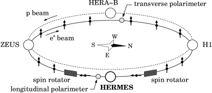
Figure 2: Schematic diagram of the HERA accelerator layout until 2000 with the location of the four experiments. Also shown are the locations of the spin–rotators and the two polarimeters.

The electron/positron beam at HERA is self–polarized by the Sokolov–Ternov mechanism Sokolov and Ternov (1964), which exploits a slight asymmetry in the emission of synchrotron radiation, depending on whether the spin of the electron/positron in the spin flip associated with the emission is parallel or anti–parallel to the magnetic guide field. This very small asymmetry (one part in $10^{10}$ Düren (1995)), causes the polarization of the beam to grow asymptotically, with a time constant that depends on the final polarization of the beam. This time constant is used in dedicated runs to verify the calibration of the polarimeters that measure the degree of polarization of the beam.

Polarizing the lepton beam at HERA is therefore a matter of minimizing depolarizing effects rather than one of producing an a priori polarized beam and keeping it polarized. An unpolarized beam is injected into the storage ring and polarization builds up over time, typically in 30–40 minutes.

The Sokolov–Ternov mechanism polarizes the beam in the transverse direction, i.e. the beam spin orientation is perpendicular to the momentum. The beam spin orientation is rotated into the longitudinal direction just upstream of HERMES, and is rotated back into the transverse direction downstream of the spectrometer. The locations of the spin rotators are indicated in Fig. 2.

The beam polarization is measured continuously by two instruments, both based on asymmetries in the Compton backscattering of polarized laser light from the lepton beam. The transverse polarimeter Barber et al. (1993, 1994), measures the polarization of the lepton beam at a point where it is polarized in the transverse direction. The interaction point (IP) of the polarized light with the lepton beam is located about $120\,\mathrm{m}$ downstream of the HERA West Hall (see Fig. 2). The polarimeter uses a spatial (up–down) asymmetry in the back–scattering of laser light from the polarized lepton beam. Back–scattered photons are measured in a split lead–scintillator sampling calorimeter, where the change in the position of the photons with initial circular polarization determines the polarization of the lepton beam. The calorimeter is located $70\,\mathrm{m}$ downstream of the IP.

A second polarimeter Beckmann et al. (2002) some $90\,\mathrm{m}$ downstream of the HERMES target (and just before the spin is rotated back to the transverse direction) measures the polarization of the beam when it is in the longitudinal orientation. This polarimeter is also based on Compton back–scattering of laser light, but in this case the asymmetry is in the total cross–section, and not in the spatial distribution. The larger asymmetry in this case allows a more precise measurement of the beam polarization. The higher precision is reflected in the smaller systematic uncertainties of the polarization measurements in the years 1999 and 2000. Additionally, this second polarimeter provides the possibility to measure the polarization of each individual positron bunch in HERA. This feature is particularly useful for the optimization of the beam polarization when the HERA lepton beam is in collision with the HERA proton beam. The existence of two polarimeters also allows a cross–check of the polarization measurement to be made.

The beam polarization was typically greater than $50\,\%$ in the later years of the experiment, attaining values near $60\,\%$ for many fills of the storage ring. Average beam polarizations, the precision of the polarization measurement, as well as the charge of the HERA lepton beam for each year are given in Tab. 2.

Table 2: Beam polarization and HERA lepton beam charge for each year of HERMES running covered in this paper. The numbers are weighted by the luminosity so that the value at the beginning of the fill dominates. Polarization values were larger at the end of the fill. The fractional uncertainties quoted are the ones used in the data analysis.

	Lepton	Average	Fractional
Year	beam charge	Polarization	Uncertainty
1996	$e^{+}$	$52.8\,\%$	$3.4\,\%$
1997	$e^{+}$	$53.1\,\%$	$3.4\,\%$
1998	$e^{-}$	$52.1\,\%$	$3.4\,\%$
1999	$e^{+}$	$53.3\,\%$	$1.8\,\%$
2000	$e^{+}$	$53.3\,\%$	$1.9\,\%$

III.2 Polarized Target

HERMES has used two types of polarized targets over the years. In 1995 an optically pumped polarized ³He target was installed DeSchepper et al. (1998). Since these data are not used in the present analysis, no description of this target is given here. In 1996–97, polarized hydrogen was used, while in 1998–2000 the target was polarized deuterium. In both cases, the source of polarized atoms was an atomic beam source (ABS). The ABS and the Breit–Rabi polarimeter (BRP) used to monitor the degree of polarization are described in Nass et al. (2003); Baumgarten et al. (2002a); Baumgarten et al. (2002b). A schematic diagram of the polarized target is shown in Fig. 3. Briefly, the atomic beam source is based on the Stern–Gerlach effect. Neutral atomic hydrogen or deuterium is produced in a dissociator and is formed into a beam using a cooled nozzle, collimators and a series of differential pumping stations. A succession of magnetic sextupoles and radio–frequency (RF) fields are used to select one (or two) particular atomic hyperfine states that have a given nuclear polarization.

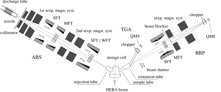
Figure 3: Diagram of the HERMES polarized target. Shown are the atomic beam source (ABS), the target gas analyzer (TGA) and the Breit–Rabi polarimeter (BRP). SFT, MFT, and WFT label the strong, medium, and weak field transitions in the ABS and the BRP.

The ABS feeds a storage cell Baumgarten et al. (2003a) which serves to increase the density by two orders of magnitude. This storage cell is located in the HERA ring vacuum and it is cooled to a temperature between $70\,\mathrm{K}$ (deuterium) and $100\,\mathrm{K}$ (hydrogen). The cell is $40\,\mathrm{cm}$ long and had elliptical cross–sectional dimensions of $29\times 9.8\,\mathrm{mm}^{2}$ in 1996–1999 and $21\times 8.9\,\mathrm{mm}^{2}$ in 2000.

The polarization and the atomic fraction of the target were monitored by sampling the gas in the target cell using the target gas analyzer (TGA) and the BRP. The TGA is a quadrupole mass spectrometer (QMS) which measures the relative fluxes of atomic and molecular hydrogen or deuterium and thereby determines the molecular fraction of the target gas. The BRP works essentially in reverse to the ABS. Single atomic hyperfine states are isolated using magnetic and RF fields and the atoms in each hyperfine state are counted using again a QMS. The electromagnetic fields are varied in a sequence such that atoms in each hyperfine state are counted in succession. More details are given in Baumgarten et al. (2002a); Baumgarten et al. (2002b); Simani (2002); Baumgarten et al. (2003b). Tab. 3 lists the target type, average polarization, and uncertainty for each data set. The differences in the systematic uncertainties are largely due to varying running conditions and the quality of the target cell in use.

Table 3: Target type and polarization for each year of HERMES running. These values are weighted by the luminosity. The uncertainty quoted is the one used in the data analysis.

		Average	Fractional
Year	Type	Polarization	Uncertainty
1996	H	$75.9\,\%$	$5.5\,\%$
1997	H	$85.0\,\%$	$3.8\,\%$
1998	D	$85.6\,\%$	$7.5\,\%$
1999	D	$83.2\,\%$	$7.0\,\%$
2000	D	$+85.1,-84.0\,\%$	$3.5\,\%$

III.3 The HERMES Spectrometer

The HERMES spectrometer is described in detail in Ackerstaff et al. (1998a). It is a forward spectrometer with large acceptance that can detect the scattered electron/positron as well as hadrons in coincidence. This allows semi–inclusive measurements of the polarized DIS process, which are the focus of this paper. A diagram of the spectrometer is shown in Fig. 4.

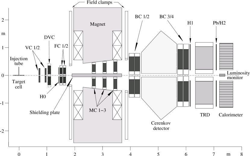
Figure 4: Side view of the HERMES spectrometer. The positron beam enters from the left. The spectrometer is split into two halves, one above the beam and one below, by a flux exclusion plate to protect the beams from the magnetic field. See the text for further details on the detectors.

Briefly, the HERMES spectrometer consists of multiple tracking stages before and after a $1.3\,\mathrm{Tm}$ dipole magnet, as well as extensive particle identification. The geometrical acceptance of the spectrometer is $\pm 170\,{\mathrm{mrad}}$ in the horizontal direction and between $\pm 40\,{\mathrm{mrad}}$ and $\pm 140\,{\mathrm{mrad}}$ in the vertical. The range of scattering angles is therefore $40\,{\mathrm{mrad}}$ to $220\,{\mathrm{mrad}}$. The spectrometer is split into two halves (top/bottom) due to the need for a flux shielding plate in the mid–plane of the magnet to eliminate deflection of the primary lepton and proton beams, which pass through the spectrometer. The lepton beam passes along the central axis of the spectrometer. The proton beam traverses the spectrometer parallel to the lepton beam but displaced horizontally by 71.4 cm.

III.3.1 Particle Tracking

The tracking system serves several functions:

• Determine the event vertex to ensure the event came from the target gas, not from the walls of the target cell or from the collimators upstream of the target.

• Measure the scattering angles of all particles.

• Measure the particle momentum from the deflection of the track in the spectrometer magnet.

• Identify hits in the PID detectors associated with each track.

The tracking system consists of 51 planes of wire chambers and six planes of microstrip gas detectors. Because of the width of the tracking detectors in the rear section of the spectrometer, it was not possible to use horizontal wires in these chambers. Instead, wires tilted $\pm 30^{\circ}$ from the vertical were used ($U$ and $V$ planes), together with vertical wires ($X$ planes). All chambers have this geometry to simplify the tracking algorithm (see below).

The majority of the tracking detectors are horizontal drift chambers with alternating anode and cathode wires between two cathode foils. The chambers are assembled in modules of six layers in three coordinate doublets ($XX^{\prime}$, $UU^{\prime}$, and $VV^{\prime}$). The primed planes are offset by a half–cell to resolve left–right ambiguities.

In order starting at the target, the tracking chambers are:

Vertex Chambers (VC1/2):

The main purpose of the vertex chambers van Hunen (1999); Blouw et al. (1999) is to measure the scattering angle to high precision and determine the vertex position of the interaction. Because of severe geometrical constraints and the high flux of particles in the region so close to the target, microstrip gas chambers (MSGC) were chosen for the VCs. Each of the upper and lower VC detectors consist of six planes grouped into two modules (VUX and XUV for VC1 and VC2 respectively). The pitch of the strips is $0.193\,\mathrm{mm}$.

Drift Vertex Chambers (DVC):

The drift vertex chambers have a cell size of $6\,\mathrm{mm}$ in each module in the $XX^{\prime}UU^{\prime}VV^{\prime}$ geometry.

Front Chambers (FC1/2):

The front chambers Brack et al. (2001) are drift chambers mounted on the front face of the spectrometer magnet. The cell size is $7\,\mathrm{mm}$ in the $XX^{\prime}UU^{\prime}VV^{\prime}$ geometry.

Magnet Chambers (MC1–3):

The magnet chambers Andreev et al. (2001) are located in the magnet gap. The MCs are proportional wire chambers with a cell width of $2\,\mathrm{mm}$. Each module consists of three planes in the $UXV$ geometry.

Back Chambers (BC1–4):

The back chambers Bernreuther et al. (1998) are large drift chambers located behind the spectrometer magnet. The cell width is $15\,\mathrm{mm}$ in the $UU^{\prime}XX^{\prime}VV^{\prime}$ geometry.

A tracking algorithm Wander (1996) defines tracks in front of and behind the magnet and the momentum of the scattered particles can therefore be determined. The MSGCs contained in the VCs were not available after 1998 due to radiation damage. In their place, vertex determination was accomplished by a refined tracking algorithm that used data from the FCs together with the point defined by the the intersection of the track in the rear of the spectrometer (the back–track) with the mid–plane of the magnet as an additional tracking parameter. The tracking algorithm is described in more detail in section IV.

Note that the magnet chambers are used only to track particles that do not reach the back of the spectrometer. They are useful for the measurement of partial tracks (mostly low–energy pions) that can, under certain conditions, increase the acceptance for the reconstruction of short–lived particles, such as $\Lambda$ particles. However, these chambers as well as the vertex and the drift vertex chambers are not used in the analysis reported in this paper.

Multiple scattering, and bremsstrahlung in the case of electrons or positrons, in the windows and other detector and target cell material which the particle tracks traverse limit the momentum resolution of the spectrometer. After its installation in 1998, the RICH detector because of its aerogel radiator assembly and heavy gas radiator increased this limit significantly. Plots of the momentum and angular resolution are shown in section IV.

III.3.2 Particle Identification

There are several particle identification (PID) detectors in the HERMES spectrometer. Electrons and positrons are identified by the combination of a lead–glass calorimeter, a scintillator hodoscope preceded by two radiation lengths of lead (the pre–shower detector), and a transition–radiation detector (TRD). A Čerenkov detector was used primarily for pion identification. The threshold detector was replaced by a Ring–Imaging Čerenkov (RICH) detector in 1998. The RICH allowed pions, kaons, and protons to be separated. Both Čerenkov detectors also helped in lepton identification.

The Calorimeter:

The calorimeter Avakian et al. (1998) has the following functions: suppress hadrons by a factor of 10 in the trigger and 100 offline; measure the energy of electrons/positrons and also of photons from other sources, e.g. $\pi^{0}$ and $\eta$ decays. It consists of two halves each containing 420 blocks (42 $\times$ 10) of radiation resistant F101 lead–glass. The blocks are $9\times 9$ cm² by 50 cm deep (about 18 radiation lengths). Each block is viewed from the back by a photomultiplier tube.

The response of the calorimeter blocks was studied in a test beam with a $3\times 3$ array. The response to electrons was found to be linear within $1\,\%$ over the energy range $1$–$30\,{\mathrm{GeV}}$. The energy resolution was measured to be $\sigma(E)/E\,[\%]=(5.1\pm 1.1)/\sqrt{E[{\mathrm{GeV}}]}+(1.5\pm 0.5)$

The Pre–Shower Detector:

The calorimeter is preceded by a scintillator hodoscope (H2) that has two radiation lengths of lead in front of it. The hodoscope H2 therefore acts as a pre–shower detector and contributes to the lepton identification. This detector consists of 42 vertical scintillator modules in each of two halves. Each paddle is $1\,\mathrm{cm}$ thick and $9.3\times 91\,\mathrm{cm}^{2}$ in area.

The lead preceding the hodoscope initiates showers for leptons but with a much reduced probability for hadrons. Pions deposit only about $2\,{\mathrm{MeV}}$ of energy on average while electrons/positrons deposit roughly $20$–$40\,{\mathrm{MeV}}$. H2 suppresses hadrons by a factor of about 10 with $95\,\%$ efficiency for detection of electrons/positrons.

Transition Radiation Detector:

The transition radiation detector (TRD) rejects hadrons by a factor exceeding 300 at $90\,\%$ electron/positron detection efficiency. Each of the upper and lower halves of the spectrometer contains six TRD modules with an active area of $325\times 75\,\mathrm{cm}^{2}$. Each module consists of a radiator and a proportional wire chamber to detect the TR photons. The radiators consist of a pseudo–random but predominantly two–dimensional array of polyethylene fibers with $17$–$20\,\mathrm{\mu m}$ diameter. The proportional chambers have a wire spacing of $1.27\,\mathrm{cm}$, use Xe:CH₄ (90:10) gas, and are $2.54\,\mathrm{cm}$ thick.

Čerenkov Detector:

In 1995–97, a threshold Čerenkov detector was operated, which was located between the two sets of back tracking chambers. During the 1996 and 1997 data taking periods, a mixture of $70\,\%$ nitrogen and $30\,\%$ C₄F₁₀ was used as the radiator, resulting in momentum thresholds for pions, kaons, and protons of 3.8, 13.6, and $25.8\,{\mathrm{GeV}}$ respectively.

As for the other components of the spectrometer, the Čerenkov detector consists of two identical units in the upper and lower half of the spectrometer. The numbers given in the following refer to one detector half. An array of 20 spherical mirrors (radius of curvature: $156\,\mathrm{cm}$) mounted at the rear of the gas volume focused the Čerenkov photons onto phototubes of diameter $12.7\,\mathrm{cm}$. Hinterberger–Winston light cones with an entrance diameter of $21.7\,\mathrm{cm}$ helped maximize light collection. The mean number of photoelectrons for a $\beta\approx 1$ particle was measured to be around five.

RICH:

The threshold Čerenkov detector was replaced in 1998 by a ring imaging Čerenkov detector (RICH) which allowed kaons and protons to be identified as well as pions Akopov et al. (2002). The RICH uses a novel two–radiator design to achieve separation of pions, kaons, and protons over the entire kinematic range of interest ($4$–$13.8\,{\mathrm{GeV}}$; see Fig. 10). One of the radiators is C₄F₁₀ gas with an index of refraction of $n=1.0014$, while the second radiator consists of aerogel tiles with index of refraction $n=1.03$ mounted just behind the entrance window. The aerogel tiles are $1.1\,\mathrm{cm}$ thick and they are stacked in five layers for a total length of $5.5\,\mathrm{cm}$. A mirror array with a radius of curvature of $220\,\mathrm{cm}$ focuses the Čerenkov photons onto $1934$ photomultiplier tubes of $1.92\,\mathrm{cm}$ diameter per detector half. Details on the analysis of the RICH data are given in section IV.

PID Detector Performance:

Plots of the responses of the PID detectors are shown in Fig. 5. A description of the PID analysis, integrating all the detectors, is given in section IV.

Figure 5: Typical PID detector responses. The distributions are based on a small set of the data collected in 2000, except for the threshold Čerenkov response, which was computed from a data set of similar size collected in 1997. The truncated mean is shown in the case of the TRD. The relative size of the lepton (dashed line) and hadron distributions (solid line) was scaled to the flux ratio in the respective data–taking periods to give a better idea of the level of contamination possible from each detector. The flux ratio of electrons to hadrons is typically $\sim 10\,\%$ for these data.

III.3.3 Event Trigger

Before discussing the trigger itself, two more detectors used specifically for the trigger must be introduced: two scintillator hodoscopes H0 and H1. The hodoscope H1 is identical to H2 except that it does not have any lead in front of it. It is situated between BC4 and the TRD. The scintillator H0 was added after the first year of running to help discriminate against particles traveling backwards in the spectrometer. These particles originate in showers initiated by the proton beam. The H0 hodoscope is placed just in front of the magnet and therefore has enough separation from H1 and H2 that it can determine whether a particle is going forward or backwards in the spectrometer.

The DIS trigger selects electron/positron events by requiring hits in the three scintillator hodoscopes (H0, H1, and H2) together with sufficient energy deposited in two adjacent columns of the calorimeter, in coincidence with the accelerator bunch signal (HERA clock). The requirement of hits in H0 and H1 suppresses neutral particle background. The calorimeter has a high efficiency for electromagnetic showers, but relatively low efficiency for hadronic showers. The calorimeter threshold was set at $1.4\,{\mathrm{GeV}}$ ($3.5\,{\mathrm{GeV}}$ for the first period in 1996).

III.3.4 Luminosity Monitor

The luminosity was measured using elastic scattering of beam particles by the electrons in the target gas: Bhabha scattering and annihilation for a positron beam, Møller scattering for an electron beam Benisch et al. (2001). The scattered particles exit the beam pipe $7.2\,\mathrm{m}$ downstream of the target. They are detected in coincidence by a pair of small calorimeters with a horizontal acceptance of $4.6$–$8.9\,{\mathrm{mrad}}$. The calorimeters consist of Čerenkov crystals of NaBi(WO₄)₂ that are highly resistant to radiation damage.

III.3.5 Data Acquisition System and Event Structure

The backbone of the data acquisition system is constructed in Fastbus. It consists of 10 front–end crates, an event collector crate, and an event receiver crate, connected to the online workstation cluster via two SCSI interfaces. CERN Host Interfaces (CHI) act as Fastbus masters, and their performance is enhanced by Struck Fastbus Readout Engines (FRE) containing two Motorola 96002 DSPs.

The drift chambers were read out by LeCroy multi–hit, multi–event 16–bit 96 channel TDCs (model 1877). Charge from the photomultipliers and from the TRD was digitized by LeCroy multi–event 64 channel 1881M multi block ADCs. These ADCs and the TDCs are capable of sparsifying the data, i.e. online suppressing channels with pedestal levels from the readout. The magnet chamber readout was instrumented with the LeCroy VME based PCOS4 system. The vertex chamber data arrived from the detector as a 16 bit ECL STR330/ECL data stream and were processed in one of the VC DSPs. Double buffering was implemented in the dual DSPs of the Fastbus masters. Event collection on one DSP was done in conjunction with readout from the second DSP to the DAQ computer.

In addition to the standard readout, a series of asynchronous independent events from the luminosity monitor and from monitoring equipment could be read out at rates exceeding $5\,\mathrm{kHz}$. One VME branch with 4 crates and three CAMAC branches with 9 crates were used for these events. The DAQ dead–time was typically less than $10\,\%$ with a total trigger rate of about $300\,\mathrm{Hz}$.

The data are arranged into the following time structure:

• Burst: Events are grouped into bursts, defined as the interval between two successive reads of the experiment scalers. A burst is roughly $10\,\mathrm{s}$ long. Data quality is checked on the burst level.

• Run: The size of the files stored on disk and tape is adjusted so that an integral number of runs can fit on a tape. At high instantaneous luminosity, one run can be as short as $10\,\mathrm{min}$. A run is the basic unit of data for analysis. Calibration constants are applied at the run level, although not all detectors are calibrated with this time granularity.

• Fill: Runs are grouped into fills, which are simply defined as data collected during a given fill of the electron storage ring.

IV Data Analysis

IV.1 Data Quality

The data used to compute the asymmetries and multiplicities were selected by a number of quality criteria applied at the burst level:

• the beam polarization was between $30\,\%$ and $80\,\%$, and the beam current was between 5 and 50 mA. (The upper bounds are beyond values observed during data–taking. They are imposed to reject faulty records.),

• the trigger dead–time was less than $50\,\%$ and the data acquisition worked satisfactorily,

• the PID system and the tracking detectors worked properly,

• there were no high voltage trips in any of the detectors,

• the experiment was in polarized running mode,

and the target system was required to be fully operational. This requirement resulted in polarizations in excess of $75\,\%$ for both the hydrogen and deuterium targets. See Refs. Simani (2002); Wendland (2003) for more details on the selection of good quality data.

IV.2 Tracking Algorithm

Particle tracks were reconstructed using the pattern of hits in the front and back tracking systems Wander (1996). In the first step of this procedure, the partial front and back tracks, which are approximately straight lines, are reconstructed separately in each of the $U$, $V$, and $X$ orientations. The algorithm is based on a fast tree search. For each orientation, the algorithm begins by considering the entire plane and successively doubles the resolution by discarding the halves without a hit. In each step the combined patterns of all planes in a given orientation are compared to a data base of physically possible tracks and only corresponding patterns are kept. After about $11$ steps the search reaches a resolution that is sufficient for track finding. The projections in the three planes are then combined to form the partial tracks in the front and the back respectively.

The front and back tracks are associated by matching pairs that intersect in the center of the magnet within a given tolerance. For each associated pair, the front track is forced to agree with the magnet mid–point of the back track, and the front track is recomputed accordingly. This procedure improves the resolution of the front tracking system, which relies on the FC chambers since only they were installed and operational during the entire data taking period from 1996 until 2000. Because the tracking information from the other chambers was not available for this entire period, they were not used in order to avoid possible biases for different data taking periods. The particle momentum is determined using another data base of $520,000$ tracks which contains the momentum as a function of the front and back track parameters. Multiple scattering in the spectrometer material leads to reduced resolutions of less than $0.03$ for the reconstructed track momenta and less than $1.5\,{\mathrm{mrad}}$ for the reconstructed scattering angles. Fig. 6 shows the resolutions for the deuterium data sample as obtained from a Monte Carlo simulation of the entire spectrometer. The momentum and angular resolution of the hydrogen data are better, because of the shorter radiation length of the Čerenkov detector compared to the RICH.

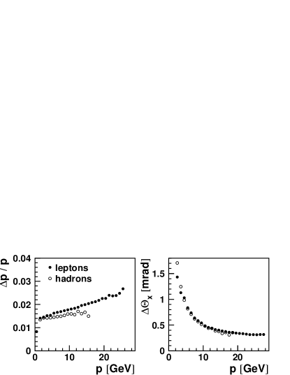
Figure 6: Tracking system resolution for lepton and hadron tracks for the detector configuration used since 1998. In the left panel the relative momentum resolution is displayed, and the right panel shows the resolution in the horizontal scattering angle $\theta_{x}$, both as a function of the track momentum $p$.

IV.3 Particle Identification Algorithm

The PID system discriminates between electrons/positrons (referred to as leptons in the following), pions, kaons, and other hadrons. It provides a factor of about 10 in hadron suppression at the trigger level to keep data acquisition rates reasonable. The hadron rate from photo production exceeds the DIS rate by a factor of up to 400:1 in some kinematic regions. In offline analysis, the HERMES PID system suppresses hadrons misidentified as leptons by as much as $10^{4}$ with respect to the total number of hadrons, while identifying leptons with efficiencies exceeding $98\,\%$.

The identification of hadrons and leptons is based on a Bayesian algorithm that uses the conditional probability $P(A|B)$ defined as the probability that $A$ is true, given that $B$ was observed. For each track the conditional probability $P(H_{l(h)}|E,p,\theta)$ that the track is a lepton (hadron) is calculated as

$$P(H_{l(h)}|E,p,\theta)=\frac{P(H_{l(h)}|p,\theta)\;P(E|H_{l(h)},p)}{\sum_{i=l,h}P(H_{i}|p,\theta)\;P(E|H_{i},p)}\,.$$ (23)

Here $H_{l(h)}$ is the hypothesis that the track is a lepton (hadron), $E$ the response of the considered detector, and $p$ and $\theta$ are the track’s momentum and polar angle. The parent distributions $P(E|H_{l(h)},p)$ of each detector (i.e. the typical detector responses) were extracted from data with stringent restrictions on the other PID detectors to isolate a particular particle type. See Fig. 5 for plots of the individual PID detector responses.

In a first approximation, uniform fluxes $P(H_{l}|p,\theta)=P(H_{h}|p,\theta)$ are assumed so that the ratio

$$\log_{10}\frac{P(H_{l}|E,p,\theta)}{P(H_{h}|E,p,\theta)}$$ (24)

reduces to:

$$\mathrm{PID}_{det}=\log_{10}\frac{P(E|H_{l},p)}{P(E|H_{h},p)}\,.$$ (25)

The quantity PID_det is defined for the calorimeter ($cal$), the pre–shower detector ($pre$), the Čerenkov detector ($cer$) (the RICH detector ($ric$) since 1998), and the TRD ($trd$). In the case of the RICH and the TRD this ratio is the sum over the $\mathrm{PID}$ values of the two radiators and the six TRD modules respectively. The $\mathrm{PID}$ distribution of the TRD ($\mathrm{PID5}$) is shown in Fig. 7 versus the sum of the $\mathrm{PID}$ values of the calorimeter, the pre–shower, and the threshold Čerenkov/RICH ($\mathrm{PID3}$). The leptons (small bump) are seen to be clearly separable from the hadrons (large peak).

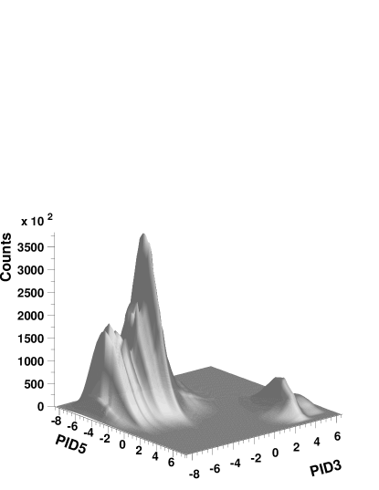
Figure 7: Two–dimensional distribution of PID values for all particles in the acceptance. The quantities $\mathrm{PID3}$ and $\mathrm{PID5}$ are defined as $\mathrm{PID3}\equiv\mathrm{PID}_{cal}+\mathrm{PID}_{pre}+\mathrm{PID}_{ric}$ and $\mathrm{PID5}\equiv\mathrm{PID}_{trd}$.

The particle fluxes $P(H_{l(h)}|p,\theta)$ were computed in an iterative procedure by comparing the calculated ratio Eq. (24) to data and varying the fluxes. These fluxes were then combined with $\mathrm{PID3+PID5}$ to form the total $\mathrm{PID}$ value

$$\mathrm{PID}=\mathrm{PID3}+\mathrm{PID5}-\log_{10}\Phi\,,$$ (26)

where $\Phi=P(H_{h}|p,\theta)/P(H_{l}|p,\theta)$ is the ratio of hadron and lepton fluxes. A plot of the quantity PID which was used to discriminate hadrons and leptons is shown in Fig. 8, where the two peaks for hadrons and leptons are seen to be well separated. Hadrons and leptons were identified with limits requiring $\mathrm{PID}<0$ and $\mathrm{PID}>1$ respectively.

Figure 8: The distribution of the total $\mathrm{PID}$ value. This logarithmic ratio of probabilities includes the particle fluxes and the responses of all PID detectors. The left hand peak is the hadron peak, while the right hand peak originates from leptons. The limits that were applied in the analysis are shown as vertical lines.

The lepton restriction provided excellent discrimination of DIS leptons from the large hadron background, with efficiencies larger than $98\,\%$ and contaminations below $1.0\,\%$ over the entire range in $x$ (see Fig. 9). Semi–inclusive hadrons were identified with efficiencies larger than $99\,\%$ and lepton contaminations smaller than $1.0\,\%$, which were determined Wendland (2003) from data collected during the normal operation of the experiment.

Figure 9: Identification efficiency and hadron contamination of the DIS lepton sample as a function of $x$. Because correlations between the responses of the PID detectors were neglected, the contaminations are uncertain by a factor of two. The deuteron data have slightly worse efficiencies and contaminations because of the better hadron–lepton discrimination of the threshold Čerenkov counter compared to the RICH.

IV.4 The Čerenkov detectors and hadron identification

The threshold Čerenkov detector identified pions with momenta between $4$ and $13.8\,{\mathrm{GeV}}$. A hadron track was identified as a pion, if the number of detected photo–electrons was above the noise level. The contamination of the pion sample by other hadrons as well as leptons is negligible.

The RICH detector identifies pions, kaons, and protons in the momentum range $2\,{\mathrm{GeV}}<p<15\,{\mathrm{GeV}}$. In the semi–inclusive analysis reported in this paper a momentum range of $4\,{\mathrm{GeV}}<p<13.8\,{\mathrm{GeV}}$ was used for consistency with the threshold Čerenkov detector. The pattern of Čerenkov photons emitted by tracks passing through the aerogel or the gas radiators on the photomultiplier matrix was associated with tracks using inverse ray tracing. For each particle track, each hadron hypothesis, and each hypothesis for the radiator emitting the photons, aerogel or gas, the photon emission angle was computed. The average Čerenkov angles $\langle\theta\rangle^{a,g}_{\pi,K,p}$ were calculated for each radiator ($a,g$) and particle hypothesis ($\pi,K,p$) by including only photons with emission angles within $2\,\sigma_{\theta}$ about the theoretically expected emission angle $\theta^{\mathrm{theo};a,g}_{\pi,K,p}$, where $\sigma_{\theta}\simeq 8\,{\mathrm{mrad}}$ is the single photon resolution. This procedure rejects background photons, and photons due to other tracks or the other radiator. Fig. 10 shows the distribution of angles in the two radiators as a function of the particle momentum.

Figure 10: Čerenkov angles associated with the three particle hypotheses as a function of the particle momentum. The characteristic angles of Čerenkov light emitted in the aerogel ($n=1.03$) are given by the solid lines. The characteristic angles for emission in the gas ($n=1.0014$) are shown as the dashed lines. The corresponding histogram entries are experimentally determined angles of a sample of SIDIS hadrons.

Based on the Gaussian likelihood,

$$\mathcal{L}^{a,g}_{i}=\exp\left[-\left(\theta^{\mathrm{theo};a,g}_{i}-\langle\theta\rangle^{a,g}_{i}\right)^{2}\frac{1}{2\sigma^{2}_{\langle\theta\rangle^{a,g}_{i}}}\right]$$ (27)

a particle hypothesis $i=\pi,K,p$ with the largest total likelihood $\mathcal{L}_{i}^{\mathrm{tot}}=\mathcal{L}_{i}^{a}\cdot\mathcal{L}_{i}^{g}$ is assigned to each hadron track.

Identification efficiencies and probabilities for contamination of hadron populations from misidentification of other hadrons were estimated with a Monte Carlo simulation which had been calibrated with pion and kaon tracks from experimentally reconstructed $\rho^{0}$, $\phi$, $K_{s}^{0}$ meson and $\Lambda$ hyperon decays. In the analysis, each pion and kaon track was assigned a weight $\omega_{i}^{K,\pi}$ accordingly. The number of counts of pions and kaons,

$$N_{K,\pi}=\sum_{i}\omega_{i}^{K,\pi}$$ (28)

were computed as the sums of these weights.

V Asymmetries

V.1 Measured Asymmetries

In the data sample that satisfied the data quality criteria described in the previous section, events were selected for analysis if they passed the DIS trigger (see section III). Tracks with a minimum energy of $3.5\,{\mathrm{GeV}}$ in the calorimeter that were identified as leptons by the PID system were selected as candidates for the scattered DIS particle by imposing additional requirements on the track kinematics. A requirement of $Q^{2}>1\,{\mathrm{GeV}}^{2}$ selected hard scattering events. Events from the nucleon resonance region were eliminated by requiring $W^{2}>10\,{\mathrm{GeV}}^{2}$. The requirement $y<0.85$ reduced the number of events with large radiative corrections.

Hadron tracks coincident with the DIS positron were identified as semi–inclusive hadrons if the fractional energy $z$ of the hadron was larger than $0.2$ and $x_{F}$ was larger than $0.1$. These limits suppress contributions from target fragmentation. Hadrons from exclusive processes, such as diffractive vector meson production, were suppressed by requiring that $z$ be smaller than $0.8$.

The final statistics of inclusive DIS events and SIDIS hadrons are given in Tab. 4. The numbers are presented in terms of statistically equivalent numbers of events $N_{\mathrm{eq}}$. This quantity is the number of unweighted events with the same relative error as the sum of weighted events $N$,

$$\frac{\sigma_{N_{\mathrm{eq}}}}{N_{\mathrm{eq}}}\equiv\frac{\sqrt{N_{\mathrm{eq}}}}{N_{\mathrm{eq}}}=\frac{\sqrt{\sum_{i}(\omega_{i})^{2}}}{\sum_{i^{\prime}}\omega_{i^{\prime}}}\equiv\frac{\sigma_{N}}{N}\,.$$ (29)

The weights $\omega_{i}$ are defined in section IV.4 for hadrons identified by the RICH detector in semi–inclusive events. For pions identified by the threshold Čerenkov counter, for undifferentiated hadrons, and for inclusive DIS events $\omega_{i}=1$. An additional weight factor of $\pm 1$ is applied according to the event classification as signal or charge–symmetric background (see below).

Table 4: Statistically equivalent number of counts of DIS events and SIDIS hadrons for the hydrogen and the deuterium data.

		SIDIS events
Target	DIS evts.	$\pi^{+}$	$\pi^{-}$	$K^{+}$	$K^{-}$
H	$1.7\times 10^{6}$	$117\times 10^{3}$	$82\times 10^{3}$
D	$6.7\times 10^{6}$	$491\times 10^{3}$	$385\times 10^{3}$	$76\times 10^{3}$	$33\times 10^{3}$

The inclusive (semi–inclusive) data samples were used to calculate the measured positron–nucleon asymmetry $A^{(h)}_{\|}$ in bins of $x$ (or $z$),

$$A_{\|}^{(h)}=\frac{N_{(h)}^{\stackrel{{\scriptstyle\rightarrow}}{{\Leftarrow}}}L^{\stackrel{{\scriptstyle\rightarrow}}{{\Rightarrow}}}-N_{(h)}^{\stackrel{{\scriptstyle\rightarrow}}{{\Rightarrow}}}L^{\stackrel{{\scriptstyle\rightarrow}}{{\Leftarrow}}}}{N_{(h)}^{\stackrel{{\scriptstyle\rightarrow}}{{\Leftarrow}}}L_{P}^{\stackrel{{\scriptstyle\rightarrow}}{{\Rightarrow}}}+N_{(h)}^{\stackrel{{\scriptstyle\rightarrow}}{{\Rightarrow}}}L_{P}^{\stackrel{{\scriptstyle\rightarrow}}{{\Leftarrow}}}}\,.$$ (30)

Here $N^{\stackrel{{\scriptstyle\rightarrow}}{{\Rightarrow}}}$ ($N^{\stackrel{{\scriptstyle\rightarrow}}{{\Leftarrow}}}$) is the number of DIS events for target spin orientation parallel (anti–parallel) to the beam spin orientation, and $N_{h}^{\stackrel{{\scriptstyle\rightarrow}}{{\Rightarrow}}}$ ($N_{h}^{\stackrel{{\scriptstyle\rightarrow}}{{\Leftarrow}}}$) are the corresponding numbers of semi–inclusive DIS hadrons. The luminosity $L^{\stackrel{{\scriptstyle\rightarrow}}{{\Rightarrow}}}$ ($L^{\stackrel{{\scriptstyle\rightarrow}}{{\Leftarrow}}}$) for the parallel (anti–parallel) spin state is corrected for dead time, while $L_{P}^{\stackrel{{\scriptstyle\rightarrow}}{{\Rightarrow}}}$ ($L_{P}^{\stackrel{{\scriptstyle\rightarrow}}{{\Leftarrow}}}$) is the luminosity corrected for dead time and weighted by the product of beam and target polarizations for the parallel (anti–parallel) spin state. Values for the beam and target polarizations are given in Tabs. 2 and 3. The bins in $x$ used in the analysis are defined in Tab. 5.

Table 5: The bins in $x$ used in the analyses presented in this paper.

bin	1	2	3	4	5	6	7	8	9
$x_{\mathrm{low}}$	0.023	0.040	0.055	0.075	0.1	0.14	0.2	0.3	0.4
$x_{\mathrm{up}}$	0.040	0.055	0.075	0.1	0.14	0.2	0.3	0.4	0.6

In the deuteron — a spin–1 particle — another polarized structure function $b_{1}^{d}$ arises from binding effects associated with the D-wave component of the ground state Hoodbhoy et al. (1989). This structure function may contribute to the cross section if the target is polarized with a population of states with spin–projection $S_{z}=0$ that is not precisely 1/3, i.e. a substantial tensor polarization. Because the maximum vector polarization can only be accomplished with a high tensor polarization in a spin 1 target, measurements in HERMES, of necessity, can include significant contributions from the tensor analyzing power of the target. For inclusive scattering, the spin asymmetry is of the form

$$A_{1}=\frac{\sigma_{1/2}-\sigma_{3/2}}{\sigma_{1/2}+\sigma_{3/2}}[1+\frac{1}{2}TA_{T}]$$ (31)

where $T$ is the tensor polarization, and $A_{T}$ is the tensor analyzing power. The $b_{1}$ structure function is measured by $A_{T}$, i.e. $A_{T}\approx 2b_{1}/3F_{1}$. Studies by the HERMES collaboration indicate that $b_{1}^{d}$ is small Contalbrigo (2002), and that the tensor contribution to the the inclusive deuteron asymmetry is less than $\approx 0.5-1.0\%$ of the measured asymmetry. For this reason, tensor contributions were assumed to be negligible for all the spin asymmetries presented here.

V.2 Charge–Symmetric Background

The particle count rates were corrected for charge symmetric background processes (e.g. $\gamma\rightarrow e^{+}+e^{-}$). The rate for this background was estimated by considering lepton tracks with a charge opposite to the beam charge that passed the DIS restrictions. It was assumed that these leptons stemmed from pair–production processes. The rate for the charge symmetric background process (where the particle is detected with the same charge as the beam but originating from pair production) is the same. The number of events with an opposite sign lepton is therefore an estimate of the number of charge symmetric events that masquerade as DIS events. They were subtracted from the inclusive DIS count rate. Hadrons that were coincident with the background DIS track and that passed the SIDIS limits were also subtracted from the corresponding SIDIS hadron sample. The DIS background rate was $\sim 6\,\%$ with respect to the total DIS rate in the smallest $x$–bin, falling off quickly with increasing $x$. The overall background fraction from this source was $1.4\,\%$.

V.3 Azimuthal Acceptance Correction

The measured semi–inclusive asymmetries were corrected for acceptance effects due to the nonisotropic azimuthal acceptance of the spectrometer. These acceptance effects arise because of an azimuthal dependence of the polarized and unpolarized semi–inclusive cross sections due, e.g. to non–zero intrinsic transverse parton momenta Mulders and Tangerman (1996). Taking into account the azimuthal dependence, the measured semi–inclusive asymmetry given in Eq. (30) is modified Oganessyan et al. (2003),

$$\frac{A_{\|}^{h}+\frac{C_{1}}{C_{0}}\langle\cos\phi\rangle_{LL}}{1+\frac{C_{1}}{C_{0}}\langle\cos\phi\rangle_{UU}}=\frac{N_{(h)}^{\stackrel{{\scriptstyle\rightarrow}}{{\Leftarrow}}}L^{\stackrel{{\scriptstyle\rightarrow}}{{\Rightarrow}}}-N_{(h)}^{\stackrel{{\scriptstyle\rightarrow}}{{\Rightarrow}}}L^{\stackrel{{\scriptstyle\rightarrow}}{{\Leftarrow}}}}{N_{(h)}^{\stackrel{{\scriptstyle\rightarrow}}{{\Leftarrow}}}L_{P}^{\stackrel{{\scriptstyle\rightarrow}}{{\Rightarrow}}}+N_{(h)}^{\stackrel{{\scriptstyle\rightarrow}}{{\Rightarrow}}}L_{P}^{\stackrel{{\scriptstyle\rightarrow}}{{\Leftarrow}}}}\,,$$ (32)

where $\langle\cos\phi\rangle_{LL}$ and $\langle\cos\phi\rangle_{UU}$ are the $\cos\phi$ moments of the semi–inclusive polarized and unpolarized cross section, respectively and $C_{0}$ and $C_{1}$ are the lowest order Fourier coefficients of the spectrometer’s azimuthal acceptance.

The semi–inclusive asymmetries $A_{\|}^{h}$ were corrected for the unpolarized moment $\langle\cos\phi\rangle_{UU}$ using a determination of the moments from HERMES data. The polarized moment $\langle\cos\phi\rangle_{LL}$ was found to be negligible as expected in Ref. Oganessyan et al. (2003). The correction for the unpolarized moment to the asymmetries is $10\,\%$ for $x<0.1$. In the measured $x$ range the absolute correction of the semi–inclusive asymmetries is small, because of the small size of the asymmetries at low $x$ (see below) and because the correction is small for $x>0.1$. The correction to the asymmetries as function of $z$ is about $10\,\%$ at small $z$ and becomes smaller for larger values of $z$.

V.4 Radiative and Detector Smearing Effects

The asymmetries were corrected for detector smearing and QED radiative effects to obtain the Born asymmetries which correspond to pure single photon exchange in the scattering process. The corrections were applied using an unfolding algorithm that accounts for the kinematic migration of the events. As opposed to iterative techniques described in Ref. Akushevich and Shumeiko (1994) for example, this algorithm does not require a fit of the data. The final Born asymmetries shown in Figs. 13 and 14 depend only on the measured data, on the detector model, on the known unpolarized cross sections, and on the models for the background processes. Another advantage is the unambiguous determination of the statistical variances and covariances on the Born asymmetries based on the simulated event migration. A description of the unfolding algorithm and the input Monte Carlo data is found in App. A.

Figure 11: The observed asymmetries $A_{\|}$ and $A_{\|}^{\pi^{+}}$ on the proton target compared with the corresponding Born asymmetries. The Born asymmetries are offset horizontally for better presentation. See the text for details.

Figure 12: Uncertainty inflation caused by detector smearing and QED radiative effects. The left hand panel shows the uncertainty inflation of the inclusive asymmetry for the proton and the right hand panel that of the positive pion asymmetry. In both panels the open triangles present the uncertainty inflation caused by detector effects, the open squares present the inflation caused by QED radiative effects, and the filled circles show the total uncertainty inflation.

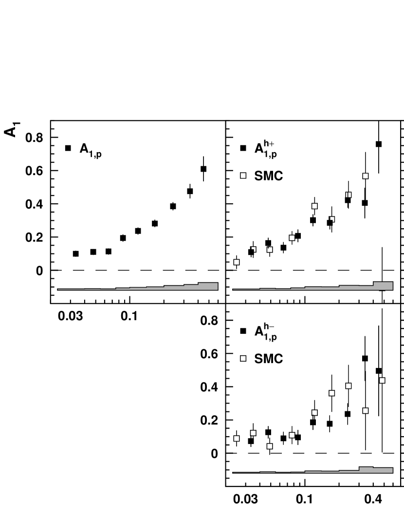
Figure 13: The inclusive and semi–inclusive Born level asymmetries on the proton, corrected for instrumental smearing and QED radiative effects. The error bars give the statistical uncertainties, and the shaded bands indicate the systematic uncertainty. The open squares show the positive and negative hadron asymmetries measured by the SMC collaboration, limited to the HERMES $x$–range Adeva et al. (1998b).

The impact of the unfolding on the asymmetries is illustrated with the inclusive and the positive pion asymmetries on the proton in Fig. 11. The unfolding procedure shifts the central asymmetry values only by a small amount. This is expected for cross section asymmetries. Smearing results in a loss of information about more rapid fluctuations that may be present in the data. Therefore correcting for this loss by effectively enhancing “higher frequency” components inevitably results in an inflation of the uncertainty of each data point. The uncertainty inflation introduced by the unfolding is shown in Fig. 12. The uncertainty at low $x$ is significantly increased by the QED background in the case of the inclusive asymmetry. At large values of $x$ and in the case of the semi–inclusive asymmetries, the inflation by QED radiation is mainly due to inter–bin event migration. Detector smearing effects, which are largest at high $x$, increase the uncertainties through inter–bin migration and a small number of events that migrate into the acceptance. Uncertainty inflation due to interbin migration increases rapidly as the bin size is reduced to be comparable to the instrumental resolution.

It should be noted that this unfolding procedure is more rigorous than the procedure applied in previous DIS experiments and previous analyses of this experiment. The size of the uncertainties is larger in the current analysis due to the explicit inclusion of correlations between $x$–bins and the model–independence of the unfolding procedure. This should be borne in mind when comparing the current data to other results.

V.5 Results for the Asymmetries

The asymmetries $A^{(h)}_{\|}$ are related to the inclusive and semi–inclusive photon–nucleon asymmetries $A^{(h)}_{1}$ through the kinematical factors $\eta$ and $\gamma$ and the depolarization factor $D$ (see Eq. (13)). The Born level asymmetries $A_{1}^{(h)}$ on the proton and on the deuteron targets are shown in Figs. 13 and 14 and are listed in Tabs. 12 and 13 in App. B, respectively. The present results on the proton target supersede earlier results published in Ackerstaff et al. (1999).

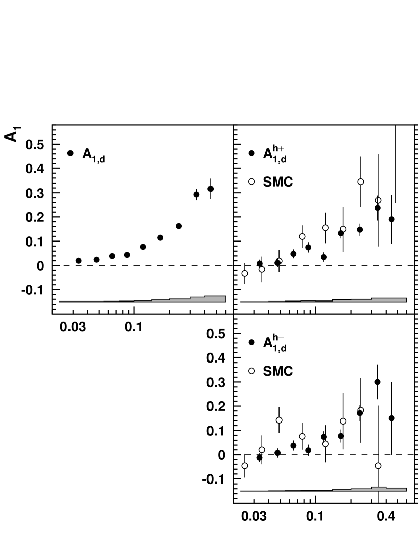
Figure 14: The inclusive and semi–inclusive Born level asymmetries on the deuteron. One data point at $x=0.45$ for the $K^{-}$ asymmetry including its large error bar is outside the displayed range; all data points are listed in Tab. 13. See Fig. 13 for details.

The inclusive asymmetries on the proton and the deuteron are determined with high precision. On both targets, they are large and positive. A detailed discussion and a determination of the spin structure functions $g_{1}$ from inclusive scattering data is given in Ref. Airapetian et al. (1998) for the proton and a forthcoming paper in the case of the deuteron.

The asymmetries for undifferentiated positive and negative hadrons on both targets are compared with measurements performed by the SMC collaboration Adeva et al. (1998b). The statistical uncertainties of the HERMES data are significantly better than those of the SMC data. Pion asymmetries on the proton and pion and kaon asymmetries on the deuteron were measured for the first time. The pion asymmetries are determined with good precision, whereas the kaon asymmetries have larger statistical uncertainties. Except for the $K^{-}$ asymmetry, all asymmetries are seen to be mostly positive, which is attributed to the dominance of scattering off the $u$–quark. The fragmentation into negative kaons ($\bar{u}s$–mesons) has in comparison to the other hadrons an increased sensitivity to scattering off $\bar{u}$ and $s$–quarks, which makes the $K^{-}$ asymmetry a useful tool to determine the polarization of these flavors.

V.6 $z$–Dependence of the Asymmetries

Because the ratio of favored to unfavored fragmentation functions is known to vary substantially with $z$, a $z$–dependence of the asymmetries could be induced by the variation of the relative contributions of the various quark flavors to fragmentation. The observation of a $z$–dependence of the asymmetries could also be caused by hadrons in the semi–inclusive data sample that originate from target fragmentation as opposed to current fragmentation, which is associated with the struck quark. Furthermore, hadrons from non–partonic processes such as diffractive interactions could play an important role in the semi–inclusive DIS data sample Szczurek et al. (2001). For example, at high fractional energies $z$, it is possible that hadrons from exclusive processes are misinterpreted as SIDIS hadrons.

Figure 15: The semi–inclusive Born asymmetries for positive and negative pion production on the proton as a function of $z$. The error bars indicate the statistical uncertainties and the error band represents the systematic uncertainties. The solid line is the z dependence from the Monte Carlo simulation of the asymmetries.

To explore these possibilities, and to test the Jetset fragmentation model used here (see section VI.1) in the Monte Carlo simulation of the scattering process, the semi–inclusive asymmetries were extracted in bins of $z$. They were calculated with the same kinematical limits described above, except for the requirement on $x_{F}$, which is highly correlated with the limit on $z$ and was therefore discarded. Events were accepted over the range $0.023<x<0.6$. The semi–inclusive pion asymmetries for the proton are shown in Fig. 15 together with a curve of the asymmetries from the Monte Carlo simulation. The agreement between experimental and simulated data provide confirmation that the fragmentation process is consistently modeled.

V.7 Systematic Uncertainties in $A_{1}$

Systematic uncertainties in the observed lepton–nucleon asymmetries $A_{\|}^{(h)}$ arise from the systematic uncertainties in the beam and target polarizations. The unfolding of the observed asymmetries also increases these uncertainties. A systematic uncertainty due to the RICH hadron identification was estimated to be small as the effect of neglecting the hadron misidentification (neglecting the off–diagonal elements of $\omega$ appearing in Eq. (28)) was found to be negligible. Therefore, it was not included in the semi–inclusive deuterium asymmetries.

Table 6: The fractional systematic uncertainties on $A_{1}$ averaged over $x$.

Source	Hydrogen data	Deuterium data
Beam polarization	$4.2\,\%$	$2.3\,\%$
Target polarization	$5.1\,\%$	$5.2\,\%$
Azimuthal acc. (SIDIS)	$3.0\,\%$	$3.1\,\%$
QED rad. corr. (DIS)	$2.0\,\%$	$2.0\,\%$
QED rad. corr. (SIDIS)	$1.0\,\%$	$1.0\,\%$
Detector smearing	$2.0\,\%$	$2.0\,\%$
$R$	$1.1\,\%$	$1.1\,\%$
$g_{2}$	$0.6\,\%$	$1.4\,\%$

Additional uncertainties arise due to the finite MC statistics, when the corrections for detector smearing and QED radiation are applied. They are included in the statistical error bars in the figures and are listed in a separate column in the tables shown in the appendix.

In forming the photon–nucleon asymmetries $A_{1}^{(h)}$, systematic uncertainties due to the parameterization of the ratio $R$ and the neglect of the contribution from the second polarized structure function $g_{2}$ were included Beckmann (2000); Wendland (2003). The relative systematic uncertainties are summarized in Tab. 6. The total systematic uncertainties on the asymmetries are shown as the error bands in the figures.

The interpretation of the extracted asymmetries may be complicated by contributions of pseudo–scalar mesons from the decay of exclusively produced vector mesons, mostly $\rho^{0}$’s producing charged pions. The geometric acceptance of the spectrometer is insufficient to identify and separate these events, as typically only one of the decay mesons is detected. However, the fractional contributions of diffractive vector mesons to the semi–inclusive yields were estimated using a Pythia6 event generator Sjöstrand et al. (2001) that has been tuned for the HERMES kinematics Aschenauer et al. (in preparation). The results range from 2%(3%) at large $x$ to 10%(6%) at small $x$ for pions(kaons) for both proton and deuteron targets. Although some data of limited precision for double–spin asymmetries in $\rho^{0}$ and $\phi$ production have been measured by HERMES Airapetian et al. (2003), no information is available on the effects of target polarization on the angular distributions for the production and decay of vector mesons. Therefore it was not possible at this time to estimate the effect of the decay of exclusively produced vector mesons on the semi–inclusive asymmetries.

The measurement of asymmetries as opposed to total cross sections has the advantage that acceptance effects largely cancel. Nevertheless, the forward acceptance of the spectrometer restricts the topology of the DIS electron and the SIDIS hadron in the final state. It was suggested Bass (2003) that a resulting cutoff in transverse hadron momentum leads to a bias in the contributions of photon gluon fusion (PGF) and QCD Compton (QCDC) processes to the total DIS cross section. This bias could lead to an incorrect measurement of the polarizations of the quarks using SIDIS asymmetries. The momentum cut ($4\,{\mathrm{GeV}}<p<13.8\,{\mathrm{GeV}}$) on the coincident hadron tracks for particle identification using the Čerenkov/ RICH (cf. section IV.4) could potentially introduce further bias.

Figure 16: Born level Monte Carlo asymmetries on the proton in the experimental acceptance and in $4\pi$. The left hand plot compares the semi–inclusive asymmetries $A_{1,p}^{\pi^{+}}$ and the right hand plot the semi–inclusive asymmetries $A_{1,p}^{\pi^{-}}$. The asymmetries in the experimental acceptance also include the hadron momentum cut. For display purposes the full data points have been offset horizontally. The lower panels present the same data in the form of the difference in the asymmetries divided by the total experimental uncertainty $\sigma_{born}$ in the corresponding measured Born asymmetry.

Possible effects on the asymmetries due to the acceptance of the HERMES spectrometer were studied with the HERMES Monte Carlo simulation. Born level data were generated using a scenario in which contributions to the cross sections from PGF and QCDC processes were found to be smaller than $7\,\%$ and $18\,\%$ respectively. These values were obtained in a scheme of cut offs against divergences in the corresponding QCD matrix elements which require quark-antiquark pairs to have masses $m_{q\overline{q}}>1\,{\mathrm{GeV}}$ and $>\,0.005\,W^{2}$. This is to be compared with the default values used in the purity analysis of $m_{q\overline{q}}>2\,{\mathrm{GeV}}$ and $>\,0.005\,W^{2}$. In this default case the contributions from PGF and QCDC processes were less than $1.5\,\%$ and $3\,\%$ respectively. In the scenario employed for the acceptance study the effect of the experimental acceptance was determined to be negligible compared to the uncertainties in the data. The semi–inclusive $\pi^{+}$ and $\pi^{-}$ asymmetries in $4\pi$ and inside the acceptance are compared in Fig. 16. Acceptance effects on the Born level asymmetries are small and corrections are not necessary.

VI Quark Helicity Distributions

VI.1 Quark Polarizations and Quark Helicity Densities

A “leading order” analysis which included the PDF and QCDC processes discussed in the previous section was used to compute quark polarizations from the Born asymmetries. The contribution of exclusively produced vector mesons is not distinguished in this extraction. The analysis based on Eq. (19) combines the Born asymmetries in an over–constrained system of equations,

$$\vec{A}_{1}(x)=\left[\mathcal{N}(x)\mathcal{P}(x)\right]\vec{Q}(x)\,,$$ (33)

where the elements of the vector $\vec{A}_{1}(x)$ are the measured inclusive and semi–inclusive Born asymmetries and the vector $\vec{Q}(x)$ contains the unknown quark polarizations. The matrix $\mathcal{N}$ is the nuclear mixing matrix that accounts for the probabilities for scattering off a given nucleon in the deuteron nucleus and the nucleon’s relative polarization. The matrix $\mathcal{P}$ contains as elements the effective purities for the proton and the neutron. These elements were obtained by integrating Eq. (19) over the range in $z$ and $Q^{2}$ giving

$$A_{1}^{h}(x)=\sum_{q}{\cal P}_{q}^{h}(x)\,\frac{\Delta q(x)}{q(x)}\,,$$ (34)

where ${\cal P}_{q}^{h}(x)$ is now the effective spin–independent purity

$${\cal P}_{q}^{h}(x)=\frac{e_{q}^{2}\,q(x)\,\int_{0.2}^{0.8}D_{q}^{h}(z)\mathrm{d}z}{\sum_{q^{\prime}}\,e_{q^{\prime}}^{2}\,q^{\prime}(x)\,\int_{0.2}^{0.8}D_{q^{\prime}}^{h}(z)\mathrm{d}z}\,.$$ (35)

The vector $\vec{A}_{1}(x)$ includes the inclusive and the semi–inclusive pion asymmetries on the proton, and the inclusive and the semi–inclusive pion and kaon asymmetries on the deuteron:

$$\vec{A}_{1}(x)=\left(A_{1,p}(x),\,A_{1,p}^{\pi^{+}}(x),\,\dots,\,A_{1,d}^{K^{-}}(x)\right)\,.$$ (36)

The semi–inclusive asymmetries of undifferentiated hadrons were not included in the fit because they are largely redundant with the pion and kaon asymmetries and thus do not improve the precision of the results.

The nuclear mixing matrix $\mathcal{N}$ combines the proton and neutron purities into effective proton and deuteron purities. The relation is trivial for the proton. In the case of the deuteron purities, the matrix takes into account the different probabilities for scattering off the proton and the neutron as well as the effective polarizations of the nucleons. The probabilities were computed with hadron multiplicities measured at HERMES and using the NMC parameterization of $F_{2}$ Arneodo et al. (1995). The D–state admixture in the deuteron wave function of $(5\pm 1)\,\%$ Desplanques (1988); Machleidt et al. (1987) leads to effective polarizations of the nucleons in the deuteron of $p_{p,D}=p_{n,D}=(0.925\pm 0.015)\,p_{D}$.

The purities depend on the unpolarized quark densities and the fragmentation functions. The former have been measured with high precision in a large number of unpolarized DIS experiments. The CTEQ5L parton distributions Lai et al. (2000) incorporating these data were used in the purity determination. Much is known about fragmentation to mesons at collider energies. However, the application of this information to fixed target energies presents difficulties, especially regarding strange fragmentation, which at lower energies no longer resembles that of lighter quarks. A recent treatment Kretzer et al. (2002) using extracted fragmentation functions in an analysis of inclusive and semi–inclusive pion asymmetries for the proton demonstrates the shortcomings of using the limited avaiable data base for fragmentation functions. Hence the interpretaton of the present asymmetry data requires a description of fragmentation that is constrained by meson multiplicities measured at a similar energy. Such multiplicities within the HERMES acceptance are available, but those for kaons not yet available corrected to $4\pi$ acceptance. Hence the approach taken here was to tune the parameters of the LUND string model implemented in the Jetset 7.4 package Sjostrand (1994) to fit HERMES multiplicities as observed in the detector acceptance.

In the LUND model, mesons are generated as the string connecting the diquark remnant and the struck quark is stretched. Quark–antiquark pairs are generated at each breaking of the string. Even though the leading hadron is often generated at one of the string breaks and not at the end, the flavor composition of any hadron observed at substantial $z$ retains a strong correlation with the flavor of the struck quark. It is this correlation which provides semi–inclusive flavor tagging. Contrary to some speculations based on a misunderstanding of the Jetset code Kotzinian (2003), this feature of the Lund string model is independent of $W^{2}$ in lepton–nucleon scattering. The quarks associated with either half of the string retain the information on the flavor of the struck quark. The LUND model has proved to be a reliable widely accepted means of describing the fragmentation process.

The string breaking parameters of the LUND model were tuned to fit the hadron multiplicities measured at HERMES in order to achieve a description of the fragmentation process at HERMES energies Menden (2001).

Figure 17: Multiplicities of charged pions and kaons in the HERMES acceptance compared with Monte Carlo data as function of $z$. Statistical uncertainties in the data are too small to be visible. The multiplicities shown were not corrected for radiative and instrumental effects.

A comparison of the measured and the simulated hadron multiplicities is shown in Fig. 17. The tuned Monte Carlo simulation reproduces the positive and negative pion multiplicities and the negative kaon multiplicities while the simulated positive kaon multiplicities are smaller than those measured. A similar disagreement is also reported by the EMC experiment Arneodo et al. (1985).

The purities were computed in each $x$–bin $i$ from the described tuned Monte Carlo simulation of the entire scattering process as

$$P_{q}^{h}(x_{i})=\frac{N_{q}^{h}(x_{i})}{\sum_{q^{\prime}}N_{q^{\prime}}^{h}(x_{i})}\,.$$ (37)

In this expression, $N_{q}^{h}$ is the number of hadrons of type $h$ in bin $i$ passing all kinematic restrictions when a quark of flavor $q$ was struck in the scattering process. The purities include effects from the acceptance of the spectrometer. In Fig. 18 the purities for the proton and the neutron are shown.

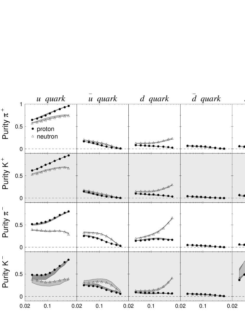
Figure 18: Purities for positive and negative pions and kaons on a proton and a free neutron target. Each column corresponds to scattering off a certain quark flavor. The shaded bands indicate the estimated systematic uncertainties due to the fragmentation parameters. The estimate derives from a comparison of two parameter sets. See text for details.

It is evident from these plots that the $u$–quark dominates the production of hadrons, due to its charge of $2/3$ and its large number density $u(x)$ in the nucleon. In particular the large contribution by the $u$–quark to $\pi^{+}$ production from both proton and neutron targets provides excellent sensitivity to the polarization of the $u$–quark. The $d$–quark becomes accessible through the production of negative pions, which also separates the $\bar{u}$ and $\bar{d}$ flavors. More generally, contributions from the sea quarks can be separated from the valence quarks through the charge of the final state hadrons. Finally the measurement of negative kaons is sensitive to strange quarks and the anti–strange quark can be accessed through positive kaons in the final state. However, large uncertainties in the strange sea distributions are expected, because the strange and anti–strange purities are small in comparison to those for the other flavors. Some of the strange quark purities vary rapidly with $Q^{2}$.

The quark polarizations $[\Delta q/q](x)$ are obtained by solving Eq. (33). A combined fit was carried out for all $x$–bins to account for the statistical correlations of the Born asymmetries (cf. Eq. (59)). Accordingly, the vectors $\vec{A}_{1}$ and $\mathcal{N}\,\mathcal{P}\vec{Q}$ are arranged such that they contain consecutively their respective values in all $x$–bins,

$$\vec{A}_{1}=\left(\vec{A}_{1}(x_{1}),\,\vec{A}_{1}(x_{2}),\,\dots,\,\vec{A}_{1}(x_{9})\right)\,,$$ (38)

and analogously for $\mathcal{N}\,\mathcal{P}\vec{Q}$. The polarizations follow by minimizing

$$\chi^{2}=\left(\vec{A}_{1}-\mathcal{N}\mathcal{P}\,\vec{Q}\right)^{T}{\cal V}^{-1}_{A}\left(\vec{A}_{1}-\mathcal{N}\mathcal{P}\,\vec{Q}\right)\,.$$ (39)

where ${\cal V}_{A}$ is the statistical covariance matrix (Eq. (59)) of the asymmetry vector $\vec{A}_{1}$. It accounts for the correlations of the various inclusive and semi–inclusive asymmetries as well as the inter–bin correlations.

The systematic uncertainties of the asymmetries were not included in the calculation of $\chi^{2}$. The dominant contribution to these uncertainties arises from the beam and target polarizations, which affect the asymmetries in a nonlinear manner. It is natural to linearly approximate these contributions as off-diagonal inter-bin correlations in the systematic covariance matrix of the set of asymmetries for all bins. However, when such a matrix is included in the fit based on linear recursion, the inaccuracies in this linearization were found to introduce a significant bias in the fit. Hence, the systematic uncertainties were excluded from the fit, but were included in the propagation of all of the uncertainties in the asymmetries into those on the results of the fit.

It was found that the data do not significantly constrain $\Delta\bar{s}(x)$. The results presented here were extracted with the constraint $\Delta\bar{s}(x)\equiv 0$. A comparison of the fit using this constraint with a fit without assumptions on the polarizations of the quark flavors showed that the constraint had negligible impact on the final results for the unconstrained flavors and their uncertainties. In addition the resulting polarizations were found to be in good agreement with the results of a fit under the assumption of a symmetrically polarized strange sea $[\Delta{s}/s](x)=[\Delta{\bar{s}}/\bar{s}](x)$.

Assuming an unpolarized anti–strange sea the vector of polarizations $\vec{Q}(x)$ in each $x$–bin is given by

$$\vec{Q}(x)=\left(\frac{\Delta u}{u}(x),\,\frac{\Delta d}{d}(x),\,\frac{\Delta\bar{u}}{\bar{u}}(x),\,\frac{\Delta\bar{d}}{\bar{d}}(x),\,\frac{\Delta s}{s}(x)\right)\,.$$ (40)

As a further constraint the polarizations of the $\bar{u}$, $\bar{d}$, and $s$–quarks were fixed at zero for values of $x>0.3$. The effects of this and of fixing the $\bar{s}$ polarization at zero were included in the systematic error. The constraints reduced the number of free parameters by fifteen, leaving $39$ parameters in the fit. The solution obtained by applying linear regression is

$$\vec{Q}=\left({\cal P}^{T}_{ef}({\cal V}_{A})^{-1}{\cal P}_{ef}\right)^{-1}{\cal P}^{T}_{ef}({\cal V}_{A})^{-1}\vec{A^{\prime}_{1}},$$ (41)

where $\vec{A^{\prime}_{1}}\equiv\vec{A}_{1}-{\cal N}{\cal P}\vec{Q}_{fix}$, ${\cal P}_{ef}\equiv{\cal N}{\cal P}$, and $\vec{Q}_{fix}$ is the set of constrained polarizations. The covariance matrix of the quark polarizations propagated from the Born asymmetries is

$${\cal V}(\vec{Q})= \left[\left({\cal P}^{T}_{ef}({\cal V}_{A})^{-1}{\cal P}_{ef}\right)^{-1}{\cal P}^{T}_{ef}({\cal V}_{A})^{-1}\right]{\cal V}_{A}^{tot}$$ (42)

$$\times\left[({\cal V}_{A})^{-1}{\cal P}_{ef}\left({\cal P}^{T}_{ef}({\cal V}_{A})^{-1}{\cal P}_{ef}\right)^{-1}\right],$$

where the covariance matrix ${\cal V}_{A}^{tot}$ includes the statistical and the systematic covariances, ${\cal V}_{A}^{tot}={\cal V}_{A}+{\cal V}_{A}^{sy}$. The resulting solution is shown in Fig. 19. The value of the $\chi^{2}/ndf$ of the fit is $0.91$. The reasonable $\chi^{2}$ value confirms the consistency of the data set with the quark parton model formalism of section II.C. Removing the inclusive asymmetries from the fit has only a small effect on the quark polarizations and their uncertainties.

The polarization of the $u$–quarks is positive in the measured range of $x$ with the largest polarizations at high $x$ where the valence quarks dominate. The polarization of the $d$–quark is negative and also reaches the largest (negative) polarizations in the range where the valence quarks dominate. The polarization of the light sea flavors $\bar{u}$ and $\bar{d}$, and the polarization of the strange sea are consistent with zero. The values of $\chi^{2}/ndf$ for the zero hypotheses are $7.4/7$, $11.2/7$, and $4.3/7$ for the $\bar{u}$, the $\bar{d}$, and the $s$–quark, respectively.

Figure 19: The quark polarizations in the 5 parameter $\times$ 9 $x$–bins fit. The polarizations, shown as a function of $x$, were computed from the HERMES inclusive and semi–inclusive asymmetries. The error bars are the statistical uncertainties. The band represents the total systematic uncertainty, where the light gray area is the systematic error due to the uncertainties on the fragmentation model, and the dark gray area is from the contribution of the Born asymmetries.

The quark polarizations in Fig. 19 are presented at the measured $Q^{2}$–values in each bin of $x$. The $Q^{2}$–dependence is predicted by QCD to be weak and the inclusive and semi–inclusive asymmetries measured by HERMES (cf. Figs. 13, 14 and Ref. Ackerstaff et al. (1999)) and SMC Adeva et al. (1998b) at very different average $Q^{2}$ show no significant $Q^{2}$–dependence when compared to each other. The quark polarizations $[\Delta q/q](x)$ are thus assumed to be $Q^{2}$–independent.

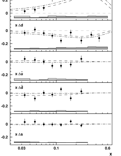
Figure 20: The quark helicity distributions $x\,\Delta q(x,Q_{0}^{2})$ evaluated at a common value of $Q^{2}_{0}=2.5\,{\mathrm{GeV}}^{2}$ as a function of $x$. The dashed line is the GRSV2000 parameterization (LO, valence scenario) Glück et al. (2001) scaled with $1/(1+R)$ and the dashed–dotted line is the Blümlein–Böttcher (BB) parameterization (LO, scenario 1) Blümlein and Böttcher (2002). See Fig. 19 for explanations of the uncertainties shown.

The quark helicity densities $\Delta q(x,Q_{0}^{2})$ are evaluated at a common $Q_{0}^{2}=2.5\,{\mathrm{GeV}}^{2}$ using the CTEQ5L unpolarized parton distributions. Because the CTEQ5L compilation is based on fits to experimental data for $F_{2}(x)$, the relationship between $F_{2}(x)$ and $F_{1}(x)$ as given by Eq. (9) is here taken into account. The factor $C_{R}\equiv(1+R)/(1+\gamma^{2})$ connects CTEQ5L tabulations with the parton distributions $q(x)$ required here. In the present analysis the parameterization for $R(x,Q^{2})$ given in Ref. Abe et al. (1999) was used. The results are presented in Fig. 20. The data are compared with two parton helicity distributions Glück et al. (2001); Blümlein and Böttcher (2002) derived from LO fits to inclusive data. The GRSV2000 parameterization, which was fitted using the assumption $R=0$, is shown with the scaling factor $1/(1+R)$ to match the present analysis. While in the Blümlein–Böttcher (BB) analysis equal helicity densities for all sea flavors are assumed, in the GRSV2000 “valence fit” a different assumption is used, which leads to a breaking of flavor symmetry for the sea quark helicity densities. In Tab. 7 the $\chi^{2}$–values of the comparison of the measured densities with these parameterizations and the zero hypothesis are given.

Table 7: Comparison of the measured quark helicity densities with the parameterizations obtained from LO QCD fits to inclusive data and with the zero hypothesis. Listed are the reduced values $\chi^{2}/ndf$ for each hypothesis.

	$x\Delta u(x)$	$x\Delta d(x)$	$x\Delta\bar{u}(x)$	$x\Delta\bar{d}(x)$	$x\Delta s(x)$
GRSV2000 val.	$1.45$	$0.93$	$1.54$	$1.44$	$0.60$
BB (scenario 1)	$1.02$	$1.06$	$0.97$	$1.32$	$0.95$
$x\Delta q(x)\equiv 0$	$13.19$	$2.50$	$1.06$	$1.60$	$0.61$
$ndf$	$9$	$9$	$7$	$7$	$7$

The measured densities are in good agreement with the parameterizations. The data slightly favor the BB parameterization of the $u$– and $\bar{u}$–flavors, while for the other flavors the agreement with both parameterizations is equally good. Within its uncertainties the measured strange density is in agreement with the very small non–zero values of the parameterizations as well as with the zero hypothesis.

The total systematic uncertainties in the quark polarizations and the quark helicity densities include contributions from the input asymmetries and systematic uncertainties on the purities, which may arise from the unpolarized parton distributions and the fragmentation model. Since the applied CTEQ5L PDFs Lai et al. (2000) are provided without uncertainties, no systematic uncertainty from this source was assigned to the purities.

The uncertainties of the fragmentation model would be ideally calculated by surveying the (unknown) $\chi^{2}$–surface of the space of Jetset parameters that were used to tune the Monte Carlo simulation. At the time of publication such a computationally intensive scan was not available. Instead the uncertainties were estimated by comparing the purities obtained using the best tune of Jetset parameters described above to a parameter set which was derived earlier Ackerstaff et al. (1999). This earlier parameter set was also obtained from a similar procedure of optimizing the agreement between simulated and measured hadron multiplicities. However, because of the lack of hadron discrimation in a wide momentum range before the availability of the RICH detector and limited available computer power, this earlier parameter tune optimized only three Jetset parameters, while in the current tune Menden (2001) eleven parameters were optimized from their default settings. The differences in the resulting purities from using these two different tunes of Jetset parameters are shown as the shaded bands in Fig. 18.

The contributions from this systematic uncertainty estimate on the purities to the total systematic uncertainties of the resulting helicity densities and quark polarizations are shown as the light shaded bands in Figs. 19, 20, and Fig. 21. In the case of the $u$ and $d$ quark, the resulting uncertainty contributions due to the fragmentation model are small compared with those related to the systematic uncertainties on the asymmetries. They are of equal or larger size in the case of the sea quarks and they dominate in case of the light sea quark helicity difference discussed in the following subsection.

VI.2 Isospin Asymmetry in Helicity Densities of Light Sea Quarks

In the unpolarized sector, the breaking of flavor symmetry for the light sea quarks $(\bar{d}(x)-\bar{u}(x)>0)$ and consequently the violation of the Gottfried sum rule is experimentally well established Baldit et al. (1994); Ackerstaff et al. (1998b); Towell et al. (2001) and is described by various non–perturbative models. Two comprehensive reviews of these models can be found in Steffens and Thomas (1997); Kumano (1998). Such models also predict a flavor asymmetry in the light sea helicity densities. Sizeable asymmetries of similar magnitude are predicted by the chiral quark soliton model ($\chi$QSM) Christov et al. (1996); Dressler et al. (2000); Diakonov et al. (1996, 1997); Wakamatsu (2003a, b), which is an effective theory where baryons appear as soliton solutions of the chiral Lagrangian, a statistical model Bourrely et al. (2002) that describes the nucleon as a gas of massless partons, models based on the meson cloud picture Fries et al. (2002); Cao and Signal (2003) as well as the chiral chromodielectric model, which is a bag–like confinement model Barone et al. (2003). The meson cloud model published in Cao and Signal (2003) deviates most from all other mentioned models as it predicts an asymmetry which is smaller in magnitude but has the opposite sign $\Delta\bar{u}(x)-\Delta\bar{d}(x)<0$ to the other models, which all predict a positive value of this quantity.

The measured (semi–)inclusive asymmetries discussed above were used in a modified fit to compute this flavor asymmetry. In this fit the parameter $[\Delta\bar{u}/\bar{u}](x)$ was replaced by $[(\Delta\bar{u}-\Delta\bar{d})/(\bar{u}-\bar{d})](x)$ and the system of linear equations (33) was solved for the following vector $\vec{Q}^{\prime}(x)$ of quark polarizations:

$$\vec{Q}^{\prime}(x)=\\ \left(\frac{\Delta u}{u}(x),\,\frac{\Delta d}{d}(x),\,\frac{\Delta\bar{u}-\Delta\bar{d}}{\bar{u}-\bar{d}}(x),\,\frac{\Delta\bar{d}}{\bar{d}}(x),\,\frac{\Delta s}{s}(x)\right)\,.$$ (43)

The flavor asymmetry $x\,[\Delta\bar{u}(x)-\Delta\bar{d}(x)]$ is presented in Fig. 21. For comparison the same quantities calculated in the $\chi$QSM Dressler et al. (2000) and in a meson cloud model Cao and Signal (2003) are shown. These models were chosen for presentation as they indicate the most positive and most negative predictions. All other cited model predictions yield similar $x$–dependences and positive values $\Delta\bar{u}(x)-\Delta\bar{d}(x)>0$. Because of the close similarity of these model curves when plotted at the scale of Fig. 21 they are not displayed in this figure.

The value of the $\chi^{2}/ndf$ for the symmetry hypothesis $\Delta\bar{u}(x)=\Delta\bar{d}(x)$ is $7.7/7$. The $\chi^{2}/ndf$ values of the comparisons with the predictions shown for the $\chi$QSM and for the meson cloud model are $17.6/7$ and $8.1/7$, respectively, where the value for the $\chi$QSM takes into account its uncertainty. This analysis of the HERMES data therefore favors a symmetric polarized light flavor sea and exclude the prediction of the $\chi$QSM at the 97% confidence level.

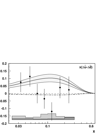
Figure 21: The flavor asymmetry in the helicity densities of the light sea evaluated at $Q_{0}^{2}=2.5\,{\mathrm{GeV}}^{2}$. The data are compared with predictions in the $\chi$QSM Dressler et al. (2000) and a meson cloud model Cao and Signal (2003). The solid line with the surrounding shaded band show the $\chi$QSM prediction together with its $\pm 1\,\sigma$ uncertainties while the dash–dotted line shows the prediction in the meson cloud model. The uncertainties in the data are presented as in Fig. 19.

VII $\Delta s$ from the Isoscalar Extraction Method

The strange quark polarization in the nucleon is one of the most interesting quantities that can be determined from SIDIS data. Kaon asymmetries provide the largest sensitivity to the strange quark polarization because the kaon contains a valence strange (anti–)quark. Unfortunately, experimental data on separate favored and disfavored fragmentation of strange quarks into kaons are scarce at best in the kinematic region of HERMES, thereby introducing large systematic uncertainties on the strange quark purities (cf. Fig. 18). This section presents an alternative approach for the extraction of the strange quark polarization, which uses only data on the asymmetry of the total ($K^{+}+K^{-}$) charged kaon flux for a deuterium target, and which does not rely on a Monte Carlo model of the fragmentation process.

The total strange quark helicity density $\Delta S(x)\equiv\Delta s(x)+\Delta\bar{s}(x)$ carries no isospin. It can hence be extracted from scattering data off a deuterium target alone, which is isoscalar. Furthermore, the fragmentation functions $D_{q=u,d,s}^{K^{+}+K^{-}}$ for the total kaon flux were measured at $e^{+}e^{-}$ collider experiments with satisfactory precision.

The analysis is performed as a two component extraction of the non–strange and total strange quark polarizations, $[\Delta Q/Q](x)$ and $[\Delta S/S](x)$. Here, $Q(x)\equiv u(x)+\bar{u}(x)+d(x)+\bar{d}(x)$. Only two measured asymmetries, the inclusive $A_{1,d}$ and the semi–inclusive $A_{1,d}^{K^{+}+K^{-}}$ asymmetries on the deuterium target, are used for the extraction. The same purity approach detailed in sections II and VI is used, except in the present case the purity matrix ${\cal P}(x)$ consists of a $2\times 2$ matrix only:

$${\cal P}(x)=\left(\begin{array}[]{cc}P_{Q}(x)&P_{S}(x)\\ P_{Q}^{K^{+}+K^{-}}(x)&P_{S}^{K^{+}+K^{-}}(x)\end{array}\right)\,.$$ (44)

Due to row–wise unitarity, there are only two independent elements in this matrix.

Based on the wealth of $e^{+}e^{-}$ collider data, parameterizations of the total charged kaon fragmentation functions $D_{q+\bar{q}}^{K^{+}+K^{-}}\!(z,Q^{2})$ are available as a function of $z$ and $Q^{2}$ Binnewies et al. (1995); Kniehl et al. (2000). The light quarks $u,d,s$ are assumed to be massless in the analyses of the $e^{+}e^{-}$ collider data Binnewies et al. (1995); Kniehl et al. (2000). This is justified in view of the high center–of–mass energies available in these experiments. However, this approximation is not valid for the lower energies available at fixed target experiments. Here, fragmentation of non–strange quarks into kaons is suppressed by an additional factor $\lambda_{s}<1$, in order to account for the lower probability to generate an $s\bar{s}$ quark pair rather than a lighter $u\bar{u}$ pair. A value of $\lambda_{s}=0.2$ was assumed for the HERMES kinematic domain, based on results from deep–inelastic muon and neutrino scattering experiments at similar center–of–mass energies Allasia et al. (1983); Arneodo et al. (1987); Adams et al. (1994). This approach allows one to compute $P_{Q}^{K^{+}+K^{-}}(x)$ directly according to Eq. (22) instead of using a Monte Carlo model of the fragmentation process. In this analysis, the elements of the $2\times 2$ purity matrix were calculated at the central kinematic values $\langle x\rangle$ and $\langle Q^{2}\rangle$ in each $x$–bin, using the LO parameterizations of the kaon fragmentation functions from Ref. Binnewies et al. (1995) and the CTEQ5L unpolarized parton densities from Ref. Lai et al. (2000).

By computing the purities from parameterizations of the fragmentation functions instead of from a Monte Carlo model, one does not take into account acceptance effects on the measured asymmetries. However, as explained in section V, the effects of the limited polar acceptance of the HERMES spectrometer on selected semi-inclusive asymmetries are negligible. The asymmetries were corrected for azimuthal acceptance effects. The precision of the method presented in this section is limited by the statistical uncertainties of the measured kaon asymmetries, and the knowledge of the strangeness suppression factor $\lambda_{s}$.

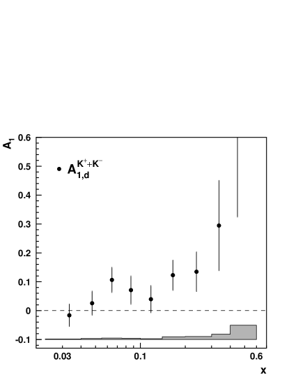
Figure 22: The semi–inclusive Born level asymmetry $A_{1,d}^{K^{+}+K^{-}}$ for the total charged kaon flux on a deuterium target, corrected for instrumental smearing and QED radiative effects. The uncertainties are presented analogously to Fig. 13.

Fig. 22 shows the semi–inclusive $K^{+}+K^{-}$ asymmetry on a deuterium target, corrected for effects of QED radiation and detector smearing, and azimuthal detector acceptance. The same kinematic limits and extraction method as described in section V were applied. The numerical values can be found in Tab. 13 in App. B. Combined with the inclusive asymmetry $A_{1,d}$ shown in Fig. 14, the total strange quark polarization $[\Delta S/S](x)$ was extracted from this data set. The average strange quark helicity density

$$\begin{split}\frac{1}{2}\left[\Delta s(x)+\Delta\bar{s}(x)\right]&=\frac{\Delta S}{S}(x)\cdot\frac{s(x)+\bar{s}(x)}{2}\\ &=\frac{\Delta S}{S}(x)\cdot s(x)\end{split}$$ (45)

is obtained by multiplication with the unpolarized strange quark density $s(x)=\bar{s}(x)$. The second equality in Eq. (45) holds because the unpolarized strange quark density is symmetric by construction for the quark and anti–quark in the parameterization employed Lai et al. (2000). The resulting average strange quark helicity density is shown in Fig. 23. In analogy to the determination of the polarizations of the sea flavors in the previous section, this extraction was restricted to the range $0.023\leq x\leq 0.3$.

The uncertainty in the strangeness suppression factor contributes the dominant part of the systematic uncertainty on the extracted values of $x\,\Delta S(x)$. It was estimated by varying $\lambda_{s}$ in the range $0.15\leq\lambda_{s}\leq 0.3$ covered by the experimental results Allasia et al. (1983); Arneodo et al. (1987); Adams et al. (1994). This contribution to the total systematic uncertainty is shown as the unshaded band in Fig. 23. The remaining contribution shown as the shaded band arises from the systematic uncertainties on the Born level asymmetries treated in the previous section.

The results from the five flavor fit to the full data set on both the proton and deuteron targets are also shown in Fig. 23.

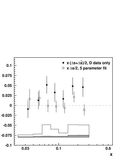
Figure 23: The average strange quark helicity density $x\cdot[\Delta s(x)+\Delta\bar{s}(x)]/2$ from the isoscalar extraction method (full points). For comparison the open symbols denote the results from a five parameter fit (see text), which are offset horizontally for presentation. The band in the bottom part gives the total systematic uncertainty on the results from the isoscalar extraction. The dark shaded area corresponds to the uncertainty from the input asymmetries, and the open part relates to the uncertainty in $\lambda_{s}$.

A comparision of the first moments of the helicity densities in the measured $x$ region provides a good measure of the agreement between the two methods. It should be noted that these two analyses use the same input data. For the five flavor fit, from Tab. 8, $\Delta s(5par)=0.028\pm 0.033\pm 0.009$. This is to be compared with $\Delta S(iso)=0.129\pm 0.042\pm 0.129$ where the systematic uncertainty is dominated by that in $\lambda_{s}$ cited above. Considering statistical and systematic uncertainties, both results are consistent with zero. (After this analysis was completed it was learned that the charged kaon multiplicities were consistent with a value somewhat larger than this range.) The helicity densities from the isoscalar method and from the full five flavor separation agree within their uncertainties. The isoscalar method yields results that are consistent with a vanishing total strange quark helicity density $[\Delta s(x)+\Delta\bar{s}(x)]=0$. In analogy to the previous section, the $\chi^{2}/ndf$ value for this hypothesis is $5.3/7$ for the results from the isoscalar extraction method. Neither the isoscalar nor the five flavor measurement provides any indication of a negative polarization of the strange sea.

VIII Moments of Helicity Distributions

VIII.1 Determination of the Moments

In the measured region, the $n$–th moment of the helicity distributions is given by

$$\Delta^{(n)}q(Q_{0}^{2})=\sum_{i}\left[\frac{\Delta q}{q}(x_{i})\int_{\xi_{i}}^{\xi_{i+1}}\!\!\!dx\>x^{n-1}\>q(x,Q_{0}^{2})\right]\,,$$ (46)

where the quark polarization $[\Delta q/q](x_{i})$ is assumed to be constant in each $x$–bin $i$ $[\xi_{i},\xi_{i+1}]$, and $q(x,Q_{0}^{2})$ is obtained from the CTEQ5L LO parameterization of the unpolarized quark densities from Ref. Lai et al. (2000) at a fixed scale of $Q_{0}^{2}=2.5\>\text{GeV}^{2}$. For simplicity, the first moment $\Delta^{(1)}q(Q_{0}^{2})$ is denoted $\Delta q(Q_{0}^{2})$ hereafter.

The simultaneous fit of all quark flavors in all $x$–bins yields the correlations between different $x$–bins as well as between different quark flavors, which are taken into account for the computation of the uncertainties on the moments. Specifically, from the solution of Eq. (39) one obtains the statistical and systematic covariance matrices ${\cal V}_{Q}^{\mathrm{stat}}$ and ${\cal V}_{Q}^{\mathrm{sys}}$ for the quark polarizations. The statistical and systematic uncertainties on the moments, $\delta^{\,\mathrm{stat}}_{\Delta q}$ and $\delta^{\,\mathrm{sys}}_{\Delta q}$, are obtained from these covariance matrices as

$$\left(\delta^{\,\mathrm{stat/sys}}_{\Delta q}\right)^{2}=\sum_{i,j}{\cal V}_{Q}^{\mathrm{stat/sys}}\!\left({\textstyle\frac{\Delta q}{q}(x_{i}),\frac{\Delta q}{q}(x_{j})}\right)\\ \times\int_{\xi_{i}}^{\xi_{i+1}}\!\!\!dx\>x^{n-1}\>q(x,Q_{0}^{2})\int_{\xi_{j}}^{\xi_{j+1}}\!\!\!dx\>x^{n-1}\>q(x,Q_{0}^{2})\,,$$ (47)

where $i$ and $j$ run over all $x$–bins. By the inclusion of the correlations between different $x$–bins the total uncertainties on the moments are reduced by 22 – 39 %, depending on the quark flavor. This can be understood as a partial compensation of the uncertainty enlargement on the asymmetries due to inter–bin event migration in the unfolding procedure (cf. section V.4 and App. A): The net migration of events from $x$–bin $i$ into $x$–bin $j$ causes these bins to be anticorrelated and hence reduces the resulting uncertainty in Eq. (47).

Theoretical predictions are often made in terms of the first moments of the isospin singlet, the isovector, and the octet combinations,

$$\Delta\Sigma =\Delta u+\Delta\bar{u}+\Delta d+\Delta\bar{d}+\Delta s+\Delta\bar{s}\,,$$ (48)

$$\Delta q_{3} =\Delta u+\Delta\bar{u}-(\Delta d+\Delta\bar{d})\,,$$ (49)

$$\Delta q_{8} =\Delta u+\Delta\bar{u}+\Delta d+\Delta\bar{d}-2(\Delta s+\Delta\bar{s})\,.$$ (50)

The resulting values in the measured range $0.023\leq x\leq 0.6$ are tabulated together with the first and second moments of the individual helicity densities in Tab. 8. For the sea flavors, the measured range is $0.023\leq x\leq 0.3$. The contributions from $0.3<x\leq 0.6$ to these moments have been fixed at zero. The valence distributions are obtained as $\Delta u_{\mathrm{v}}\equiv\Delta u-\Delta\bar{u}$ and $\Delta d_{\mathrm{v}}\equiv\Delta d-\Delta\bar{d}$. In the computation of the uncertainties of these flavor combinations the correlations between the individual helicity densities are taken into account. The corresponding statistical and systematic correlations for the first and second moments are listed in Tabs. 16 and 17 in the Appendix.

Table 8: First and second moments of various helicity distributions in the measured range at a scale of $Q_{0}^{2}=2.5\>\text{GeV}^{2}$.

	Moments in measured range
$\Delta u$	$0.601\pm 0.039\pm 0.049$
$\Delta\bar{u}$	$-0.002\pm 0.036\pm 0.023$
$\Delta d$	$-0.226\pm 0.039\pm 0.050$
$\Delta\bar{d}$	$-0.054\pm 0.033\pm 0.011$
$\Delta s$	$0.028\pm 0.033\pm 0.009$
$\Delta u+\Delta\bar{u}$	$0.599\pm 0.022\pm 0.065$
$\Delta d+\Delta\bar{d}$	$-0.280\pm 0.026\pm 0.057$
$\Delta u_{\mathrm{v}}$	$0.603\pm 0.071\pm 0.040$
$\Delta d_{\mathrm{v}}$	$-0.172\pm 0.068\pm 0.045$
$\Delta\bar{u}-\Delta\bar{d}$	$0.048\pm 0.057\pm 0.028$
$\Delta\Sigma$	$0.347\pm 0.024\pm 0.066$
$\Delta q_{3}$	$0.880\pm 0.045\pm 0.107$
$\Delta q_{8}$	$0.262\pm 0.078\pm 0.045$
$\Delta^{(2)}u$	$0.142\pm 0.009\pm 0.011$
$\Delta^{(2)}\bar{u}$	$-0.001\pm 0.005\pm 0.002$
$\Delta^{(2)}d$	$-0.049\pm 0.010\pm 0.013$
$\Delta^{(2)}\bar{d}$	$-0.003\pm 0.004\pm 0.001$
$\Delta^{(2)}s$	$0.001\pm 0.003\pm 0.001$
$\Delta^{(2)}u_{\mathrm{v}}$	$0.144\pm 0.013\pm 0.011$
$\Delta^{(2)}d_{\mathrm{v}}$	$-0.047\pm 0.012\pm 0.012$

VIII.2 Comments on Extrapolations outside the Measured Range

In order to compute the full moments for the complete $x$–range $0\leq x\leq 1$, the contributions outside the measured region would have to be estimated. For this, one has to rely on models in the kinematic regions where no data exist. In particular, the extrapolation towards $x=0$ is very problematic with many competing models making contradictory predictions Close and Roberts (1994); Bass and Landshoff (1994); Ball et al. (1995). This may be compared to the situation regarding the behavior of the unpolarized structure function $F_{2}(x,Q^{2})$ towards low values of $x$ before the HERA data became available (see for instance Bartels and Feltesse (1992)).

While in our earlier publication Ackerstaff et al. (1999) we chose one particular model (based on Regge theory), we do not pursue this approach any longer. The reason for this is the very strong model dependence which cannot be quantified reliably in terms of an associated systematic uncertainty, as some of the models yield diverging integrals in the low–$x$ range Abe et al. (1997b).

To illustrate this more clearly, we performed a study of the robustness of a global QCD fit similar to Blümlein and Böttcher (2002) (LO, scenario 1), which does include preliminary HERMES inclusive data taken on a polarized deuterium target Weiskopf (2002). In this study, the fit was repeated with artificially offset values for the parameters $\eta^{\prime}_{u_{\mathrm{v}}}=0.730$ and $\eta^{\prime}_{d_{\mathrm{v}}}=-0.270$ as compared to their default settings $\eta_{u_{\mathrm{v}}}=0.926$ and $\eta_{d_{\mathrm{v}}}=-0.341$, obtained from the constants $F$ and $D$ measured in weak neutron and hyperon $\beta$–decays. The parameterizations for the helicity densities in the QCD fit are constructed such that the parameters $\eta_{u_{\mathrm{v}}}$ and $\eta_{d_{\mathrm{v}}}$ give the first moments of the helicity valence quark distributions, $\eta_{u_{\mathrm{v}}}\equiv\int_{0}^{1}dx\;\Delta u_{\mathrm{v}}(x,Q^{2})$ and $\eta_{d_{\mathrm{v}}}\equiv\int_{0}^{1}dx\;\Delta d_{\mathrm{v}}(x,Q^{2})$.

This modification implies a $21\,\%$ change of the value of the Bjorken Sum Rule (BJSR) Bjorken (1966, 1970)

$$I_{3}\equiv\Delta q_{3}=\int_{0}^{1}\!\!dx\;\Delta q_{3}(x)=\left|\frac{g_{A}}{g_{V}}\right|$$ (51)

from its physical value $I_{3}=|g_{A}/g_{V}|=1.267$ to $I^{\prime}_{3}=1.0$. The unmodified fit agrees well with the obtained helicity distributions in the measured range as illustrated in Fig. 20 and Tab. 7 in section VI.1. This consistency is also reflected in the good agreement of the first moments in the measured range of the valence quark helicity densities $\Delta u_{\mathrm{v}}$ and $\Delta d_{\mathrm{v}}$ as well as the isotriplet flavor combination $\Delta q_{3}$ from the BB LO parameterization with the present results from semi-inclusive data, as listed in Tab. 9. It is, however, remarkable that the moments of the same quantities computed from the modified fit yield almost as good consistency with the measured results, despite the significant changes in the boundary conditions $\eta_{u_{\mathrm{v}}}$ and $\eta_{d_{\mathrm{v}}}$.

Table 9: Comparison of first moments of the LO QCD fit Blümlein and Böttcher (2002) and a modified version of it (see text) with the measured results, in the range $0.023\leq x\leq 0.6$. The values in square brackets give the absolute deviation of the moments of the QCD fits from the measured SIDIS values in units of their combined statistical and systematic uncertainties.

	Original fit		Modified fit		Measured SIDIS
$\Delta u_{\mathrm{v}}$	$0.601$	$[0.02\,\sigma]$	$0.569$	$[0.40\,\sigma]$	$0.603\pm 0.081$
$\Delta d_{\mathrm{v}}$	$-0.215$	$[0.50\,\sigma]$	$-0.220$	$[0.56\,\sigma]$	$-0.172\pm 0.082$
$\Delta q_{3}$	$0.816$	$[0.52\,\sigma]$	$0.789$	$[0.74\,\sigma]$	$0.880\pm 0.116$

While the QCD fit appears to be stable in the kinematic region where it is rather well constrained by data (the data sets entering the fit Blümlein and Böttcher (2002) cover a range $0.005\leq x\leq 0.75$) it seems to exhibit enough freedom in the unmeasured regions to allow for a drastic reduction of the total integral $I_{3}$ from $1.267$ to $1.0$. Table 10 lists the fractional contributions to the moments from the original and the modified QCD fit in the range $0<x<0.023$. In order to match the smaller value of $I_{3}^{\prime}=1.0$, the low–$x$ contributions to all moments are significantly reduced in the modified fit. In particular, the low–$x$ contribution from the original fit $\int_{0}^{0.023}\!\!dx\;\Delta q_{3}(x)=0.411$ reduces to $\int_{0}^{0.023}\!\!dx\;\Delta q_{3}^{\prime}(x)=0.178$ in the modified fit. For comparison, the high–$x$ extrapolation $\int_{0.6}^{1}dx\;\Delta q_{3}(x)=0.041$ vs. $\int_{0.6}^{1}dx\;\Delta q_{3}^{\prime}(x)=0.033$ is only slightly reduced and despite the large covered $x$–range its contribution to the total moment is small.

Table 10: Fractional contributions from the low–$x$ range $(0<x<0.023)$ to the first moments obtained from the original and modified global QCD fit (see text).

	Original fit	Modified fit
$\Delta u_{\mathrm{v}}$	$31\,\%$	$18\,\%$
$\Delta d_{\mathrm{v}}$	$36\,\%$	$18\,\%$
$\Delta q_{3}$	$32\,\%$	$18\,\%$

This study provides information about the “flexibility” of the chosen parameterizations rather than covering the full range of competing theoretical models for the extrapolations into the unmeasured kinematic regions. Yet, it demonstrates the arbitrariness of these extrapolations, in particular to the small $x$ range. In the measured region, our experimental result on $\Delta q_{3}$ agrees within $0.52\,\sigma$ with the integral of this quantity from the original QCD fit over the same $x$–range (see Tab. 9). We nevertheless refrain from interpreting this as an experimental confirmation of the BJSR Eq. (51), as the above example has shown that one can obtain a similar level of agreement with a $21\,\%$ reduction of the predicted value, thereby rendering a sound estimate of the associated systematic uncertainty impossible. For the same reason we restrict all results for the first and second moments to the experimentally covered $x$–region, albeit the weight of the low–$x$ extrapolation becomes smaller for the higher moments.

We finally remark that in Knauf et al. (2002) a reverse approach to this problem is presented, where the authors assume the validity of the BJSR Eq. (51) and use experimental data at $x>0.005$ to restrict the exponent $\lambda=-0.40\pm 0.31$ in an assumed power–like behaviour of the polarized structure function $g_{1}(x)\sim x^{\lambda}$, based on Regge theory.

VIII.3 Comparison with other Results

SMC is the only other experiment that has published results from SIDIS on the quark helicity distributions in the nucleon Adeva et al. (1998b). Due to limited statistics and the lack of discrimination between different hadron types, SMC could extract quark helicity distributions only under the assumption of $SU(3)$ flavor symmetry for the sea quark flavors, i.e. $\Delta\bar{u}(x)\equiv\Delta\bar{d}(x)\equiv\Delta s(x)\equiv\Delta\bar{s}(x)$. It is only because of this assumption that their precision in sea quark polarization is comparable to that of the present work.

The first and second moments for the valence and $\bar{u}$ sea quark helicity densities in the measured range of the HERMES data are compared in Table 11 to the results from the SMC experiment, which were integrated over the same kinematic region. It should be noted that SMC evaluated their moments according to a somewhat simpler expression Pretz (1997)

$$\Delta^{(n)}q(Q_{0}^{2})=\sum_{i}(\xi_{i+1}-\xi_{i})\>x_{i}^{n-1}\>\Delta q(x_{i},Q_{0}^{2})\,,$$ (52)

where the notations have been adapted to match the definition in Eq. (46). The integration procedure assumes constant helicity densities $\Delta q(x)$ over the entire width of an $x$–bin. In particular towards the upper experimental limit on $x$, where the $x$–bins are widest, the values determined for the helicity densities $\Delta u_{\mathrm{v}}(x)$ and $\Delta d_{\mathrm{v}}(x)$ in some cases violate the positivity limits given by the unpolarized parton densities at the upper $x$–bin limits (see Fig. 2 in Adeva et al. (1998b)). This causes larger values for the moments when computed according to Eq. (52) as compared to Eq. (46). Nevertheless the results from the two experiments are in good agreement within their combined uncertainties, while the present data set has an improved precision. When comparing the precision of the results from both experiments, note that the HERMES results are free of symmetry assumptions regarding the sea quark helicity densities and that they are based on a new unfolding technique to account for the proper propagation of uncertainties while handling QED radiative and instrumental smearing effects.

Table 11: Comparison of first and second moments in the measured range from this analysis with results from the SMC experiment. The SMC values were extrapolated to the same value of $Q_{0}^{2}=2.5\>\text{GeV}^{2}$ and integrated over the HERMES $x$–range.

	HERMES	SMC
$\Delta u_{\mathrm{v}}$	$0.603\pm 0.071\pm 0.040$	$0.614\pm 0.082\pm 0.068$
$\Delta d_{\mathrm{v}}$	$-0.172\pm 0.068\pm 0.045$	$-0.334\pm 0.112\pm 0.089$
$\Delta\bar{u}$	$-0.002\pm 0.036\pm 0.023$	$0.015\pm 0.034\pm 0.024$
$\Delta^{(2)}u_{\mathrm{v}}$	$0.144\pm 0.013\pm 0.011$	$0.152\pm 0.016\pm 0.013$
$\Delta^{(2)}d_{\mathrm{v}}$	$-0.047\pm 0.012\pm 0.012$	$-0.056\pm 0.026\pm 0.015$

IX Summary

This paper describes the most precise available measurements of semi–inclusive asymmetries in polarized deep inelastic electron/positron scattering. Results from both inclusive and semi–inclusive measurements are presented. The unique semi–inclusive data are particularly important for the unbiased extraction of sea quark helicity densities in the nucleon.

Data were collected on longitudinally polarized atomic hydrogen and deuterium gas targets. Good particle identification in the HERMES spectrometer allows hadrons that are coincident with the scattered lepton to be separated into pion and kaon samples. This gives sensitivity to the individual quark and antiquark helicity distribution functions for light and strange quark flavors.

An unfolding technique — new to this type of measurement — was applied for instrumental smearing and QED radiative effects. It takes into account event migrations between bins. This algorithm provides more rigorous, yet larger, estimates of the inflation of the uncertainties on the Born asymmetries with respect to the measured asymmetries than correction methods previously applied. The unfolding procedure also yields previously unavailable estimates of the statistical correlations between different kinematic bins. All asymmetries were found to be positive and increase with $x$, with the exception of the $K^{-}$ asymmetry which is consistent with zero over the entire measured range. The present data on undiscriminated hadrons agree well with earlier measurements by SMC at higher $Q^{2}$, albeit with much improved precision.

A “leading order” QCD analysis that relies on the technique of flavor tagging was used to extract helicity distribution functions. The results presented here allow for the first time the independent determination of five out of six quark polarizations in the nucleon. Quark polarizations $[\Delta q/q](x)$ were obtained using purities that were calculated in a Monte Carlo based on parameterizations of unpolarized parton densities and a modeling of hadron multiplicities measured at HERMES. The polarization $[\Delta u/u](x)$ was found to be positive and rising over the entire range in $x$, while $[\Delta d/d](x)$ is negative. These first results on the individual sea quark polarizations $[\Delta\bar{u}/\bar{u}](x)$, $[\Delta\bar{d}/\bar{d}](x)$, and $[\Delta s/s](x)$ are consistent with zero.

Furthermore, the “LO” approach presented here results in helicity quark distributions that are fully consistent with global QCD fits to world data on inclusive DIS asymmetries. While the BB fit favors a slightly negative strange quark helicity density $\Delta s(x)$, the data yield a small positive result. However, it should be noted that those particular fits invoke $SU(3)$ symmetry to relate the triplet $a_{3}$ and octet $a_{8}$ axial couplings to the weak decay constants $F$ and $D$, assume a $SU(3)$ symmetric sea, and require a model for the gluon helicity density $\Delta g(x)$. Because of these assumptions and taking into account the combined statistical and systematic uncertainties on the present experimental result, no significant discrepancy remains. However, the results from the present semi–inclusive scattering data might reveal the possible biases of global fits for certain quark flavors. Within the experimental uncertainty all obtained quark helicity densities $\Delta q(x)$ are in good agreement with the most recent parameterizations.

To confirm the results for the helicity distribution of the strange sea, a different isoscalar analysis leading to $\Delta s(x)+\Delta\bar{s}(x)$ was performed. This technique does not depend on a Monte Carlo modeling of the strange fragmentation functions. Instead, parameterizations of strange and non–strange fragmentation functions measured at $e^{+}e^{-}$ colliders at higher energies were utilized. The results for the two analyses are in reasonable agreement.

The first direct experimental extraction of the helicity density asymmetry $\Delta\bar{u}(x)-\Delta\bar{d}(x)$ in the light quark sea, which is predicted to be non zero by many models in analogy to the unpolarized sector ($\bar{u}(x)\neq\bar{d}(x)$), does not establish broken $SU(2)$ flavor symmetry. The data disfavor the substantial positive asymmetry predicted by the $\chi$QSM model and are consistent with the small negative asymmetry characteristic of the meson cloud model.

Moments were computed in the measured kinematic range for the quark helicity distributions and singlet and non–singlet flavor combinations. The moments of the valence and sea quark helicity densities $\Delta u_{\mathrm{v}}$, $\Delta d_{\mathrm{v}}$, and $\Delta\bar{u}$ agree with previous results from the SMC experiment. In the measured range, the non–singlet flavor combination $\Delta q_{3}$ is in good agreement with the same quantity computed from global QCD fits, which in turn by construction fulfill the Bjorken sum rule. However, because extrapolations into the unmeasured kinematic regions are not sufficiently constrained by the data reported here, an experimental confirmation of this fundamental sum rule was not possible. For the same reason we do not quote a total value for the singlet quantity $\Delta\Sigma$, which gives the total contribution from quark spins to the spin of the nucleon. In the measured range, a value of $\Delta\Sigma=0.347\pm 0.024\pm 0.066$ was obtained.

In conclusion, HERMES has made detailed semi–inclusive measurements of polarization asymmetries in deep inelastic lepton scattering. These measurements allow quark helicity distribution functions to be extracted with fewer and different model assumptions than in previous inclusive measurements.

Acknowledgements

We gratefully acknowledge the DESY management for its support, the staffs at DESY and the collaborating institutions for their significant effort. This work was supported by the FWO–Flanders, Belgium; the Natural Sciences and Engineering Research Council of Canada; the ESOP, INTAS and TMR network contributions from the European Union; the German Bundesministerium für Bildung und Forschung; the Italian Istituto Nazionale di Fisica Nucleare (INFN); Monbusho International Scientific Research Program, JSPS and Toray Science Foundation of Japan; the Dutch Foundation for Fundamenteel Onderzoek der Materie (FOM); the U.K. Particle Physics and Astronomy Research Council; and the U.S. Department of Energy and National Science Foundation.

Appendix A Unfolding of Radiative and Detector Smearing Effects

Corrections to the asymmetries for higher order QED and detector smearing effects were carried out using an unfolding algorithm as indicated in section V.4. However, the algorithm is complex, because the known absolute cross sections of the spin–dependent background processes must be normalized to the data by comparing simulated and measured unpolarized yields based on world data for $F_{2}$. The procedure uses two sets of Monte Carlo data. Born data were generated with the GRSV2000 (LO, standard scenario) spin–dependent parton distributions Glück et al. (2001) and the LUND fragmentation model implemented in Jetset 7.4 Sjostrand (1994). Within the acceptance of the HERMES spectrometer ($|\theta_{x}|<170\,\mathrm{mrad}$, $40\,\mathrm{mrad}<|\theta_{y}|<140\,\mathrm{mrad}$) an equivalent number of $11.5\,\mathrm{M}$ DIS events were generated on hydrogen and deuterium targets. The second Monte Carlo data set included, in addition, internal radiative effects and a simulation of the HERMES spectrometer. Radiative effects were simulated with RADGEN Akushevich et al. (1998), and the spectrometer simulation was done using GEANT Brun et al. (1978). An equivalent number of $5.4\,\mathrm{M}$ DIS events was available for analysis for each target. The total MC statistics are sufficiently large that the uncertainty on the Born asymmetries from this source is small (cf. Tabs. 12, 13 and 14).

Based on the latter Monte Carlo data, matrices $n_{{{\stackrel{{\scriptstyle\rightarrow}}{{\Rightarrow}}}({\stackrel{{\scriptstyle\rightarrow}}{{\Leftarrow}}})}}(i,j)$ with dimensions $n_{X}\times(n_{B}+1)$ were constructed for the parallel (${\stackrel{{\scriptstyle\rightarrow}}{{\Rightarrow}}}$) and anti–parallel (${\stackrel{{\scriptstyle\rightarrow}}{{\Leftarrow}}}$) spin–states, which describe the count rates that fall in both bin $j$ of Born kinematics and bin $i$ of eXperimental kinematics. The experimental kinematics reflect the radiative and instrumental effects. The bins $j=1,\dots,\,n_{B}$ describe the migration of DIS events, where both the experimental and the Born kinematics are within the acceptance. Here, acceptance refers to both the geometrical acceptance of the spectrometer and the phase space defined by the DIS and SIDIS cuts. The additional bin $j=0$ contains background rates that feed into the experimental bins through QED radiative and detector smearing effects. For example, in the case of the inclusive data sample on the proton, the background stems from elastic and inelastic scattering events that are radiated (through QED effects) or smeared (by interactions in the detector) into the acceptance. The experimental rates in the parallel and anti–parallel spin states in bin $i$ are given by the sum $n_{{{\stackrel{{\scriptstyle\rightarrow}}{{\Rightarrow}}}({\stackrel{{\scriptstyle\rightarrow}}{{\Leftarrow}}})}}^{X}(i)=\sum_{j=0}^{n_{B}}\,n_{{{\stackrel{{\scriptstyle\rightarrow}}{{\Rightarrow}}}({\stackrel{{\scriptstyle\rightarrow}}{{\Leftarrow}}})}}(i,j)$. The corresponding Born rates, $n_{{{\stackrel{{\scriptstyle\rightarrow}}{{\Rightarrow}}}({\stackrel{{\scriptstyle\rightarrow}}{{\Leftarrow}}})}}^{B}(j)$, in each spin state and bin $j$ were calculated from the Born Monte Carlo data.

These data, normalized with respect to each other provide access to the migration matrices ${\cal S}_{{{\stackrel{{\scriptstyle\rightarrow}}{{\Rightarrow}}}({\stackrel{{\scriptstyle\rightarrow}}{{\Leftarrow}}})}}(i,j)$, which are given by

$${\cal S}_{{{\stackrel{{\scriptstyle\rightarrow}}{{\Rightarrow}}}({\stackrel{{\scriptstyle\rightarrow}}{{\Leftarrow}}})}}(i,j)\equiv\frac{\partial\sigma^{X}_{{{\stackrel{{\scriptstyle\rightarrow}}{{\Rightarrow}}}({\stackrel{{\scriptstyle\rightarrow}}{{\Leftarrow}}})}}(i)}{\partial\sigma^{B}_{{{\stackrel{{\scriptstyle\rightarrow}}{{\Rightarrow}}}({\stackrel{{\scriptstyle\rightarrow}}{{\Leftarrow}}})}}(j)}\,,\\ \quad i=1,\dots,\,n_{X},\;j=1,\dots,\,n_{B}\,.$$ (53)

In terms of $n_{{{\stackrel{{\scriptstyle\rightarrow}}{{\Rightarrow}}}({\stackrel{{\scriptstyle\rightarrow}}{{\Leftarrow}}})}}(i,j)$ and $n_{{{\stackrel{{\scriptstyle\rightarrow}}{{\Rightarrow}}}({\stackrel{{\scriptstyle\rightarrow}}{{\Leftarrow}}})}}^{B}(j)$, these matrices can be written as

$${\cal S}_{{{\stackrel{{\scriptstyle\rightarrow}}{{\Rightarrow}}}({\stackrel{{\scriptstyle\rightarrow}}{{\Leftarrow}}})}}(i,j)=\frac{n_{{{\stackrel{{\scriptstyle\rightarrow}}{{\Rightarrow}}}({\stackrel{{\scriptstyle\rightarrow}}{{\Leftarrow}}})}}(i,j)}{n_{{{\stackrel{{\scriptstyle\rightarrow}}{{\Rightarrow}}}({\stackrel{{\scriptstyle\rightarrow}}{{\Leftarrow}}})}}^{B}(j)}\,,$$ (54)

provided the first derivatives are constant. The matrices ${\cal S}_{{{\stackrel{{\scriptstyle\rightarrow}}{{\Rightarrow}}}({\stackrel{{\scriptstyle\rightarrow}}{{\Leftarrow}}})}}$ describe the kinematical migration inside of the acceptance. Backgrounds are taken into account through the normalization with the Born rates $n_{{{\stackrel{{\scriptstyle\rightarrow}}{{\Rightarrow}}}({\stackrel{{\scriptstyle\rightarrow}}{{\Leftarrow}}})}}^{B}$ and as will be seen below in the $j=0$ row of $n_{{{\stackrel{{\scriptstyle\rightarrow}}{{\Rightarrow}}}({\stackrel{{\scriptstyle\rightarrow}}{{\Leftarrow}}})}}(i,j)$. The ${\cal S}_{{{\stackrel{{\scriptstyle\rightarrow}}{{\Rightarrow}}}({\stackrel{{\scriptstyle\rightarrow}}{{\Leftarrow}}})}}$ matrices are insensitive to the Monte Carlo model of the Born distributions, because both the numerator and the denominator scale with the relative number of Born events generated in bin number $j$.

The unknown Born rates $B_{{\stackrel{{\scriptstyle\rightarrow}}{{\Rightarrow}}}({\stackrel{{\scriptstyle\rightarrow}}{{\Leftarrow}}})}(j)$ are related to the measured asymmetries (Eq. (30) corrected for the azimuthal acceptance effects) through the migration matrices, the unpolarized experimental rates $n_{u}^{X}(i)\equiv n_{\stackrel{{\scriptstyle\rightarrow}}{{\Leftarrow}}}^{X}(i)+n_{\stackrel{{\scriptstyle\rightarrow}}{{\Rightarrow}}}^{X}(i)$ and the spin–dependent background $n_{p}(i,0)\equiv n_{\stackrel{{\scriptstyle\rightarrow}}{{\Leftarrow}}}(i,0)-n_{\stackrel{{\scriptstyle\rightarrow}}{{\Rightarrow}}}(i,0)$:

$$\sum_{j=1}^{n_{B}}\left[{\cal S}_{\stackrel{{\scriptstyle\rightarrow}}{{\Leftarrow}}}(i,j)B_{\stackrel{{\scriptstyle\rightarrow}}{{\Leftarrow}}}(j)-{\cal S}_{\stackrel{{\scriptstyle\rightarrow}}{{\Rightarrow}}}(i,j)B_{\stackrel{{\scriptstyle\rightarrow}}{{\Rightarrow}}}(j)\right]=\\ A_{\|}^{X}(i)\,n_{u}^{X}(i)-n_{p}(i,0),\quad i=1,\dots,\,n_{X}\,.$$ (55)

Here the unpolarized Born rate $B_{\stackrel{{\scriptstyle\rightarrow}}{{\Leftarrow}}}(j)+B_{\stackrel{{\scriptstyle\rightarrow}}{{\Rightarrow}}}(j)\equiv B_{u}(j)$ is known from previous experiments and incorporated in the Monte Carlo simulation: $B_{u}(j)=n_{u}^{B}(j)\equiv n_{\stackrel{{\scriptstyle\rightarrow}}{{\Leftarrow}}}^{B}+n_{\stackrel{{\scriptstyle\rightarrow}}{{\Rightarrow}}}^{B}$. The

Figure 24: Matrices $n_{u}(i,j)=n_{\stackrel{{\scriptstyle\rightarrow}}{{\Rightarrow}}}(i,j)+n_{\stackrel{{\scriptstyle\rightarrow}}{{\Leftarrow}}}(i,j)$ for DIS events and SIDIS $\pi^{+}$ events on the proton. The binning shown corresponds to the 9 bins in $x$ that were used in the asymmetry and $\Delta q$ analysis (Tab. 5). See the text for details.

background term in the sum was moved to the right hand side of the equation $n_{p}(i,0)={\cal S}_{\stackrel{{\scriptstyle\rightarrow}}{{\Leftarrow}}}(i,0)B_{\stackrel{{\scriptstyle\rightarrow}}{{\Leftarrow}}}(0)-{\cal S}_{\stackrel{{\scriptstyle\rightarrow}}{{\Rightarrow}}}(i,0)B_{\stackrel{{\scriptstyle\rightarrow}}{{\Rightarrow}}}(0)$. The rate $B_{\stackrel{{\scriptstyle\rightarrow}}{{\Rightarrow}}}(j)$ may now be eliminated in favor of $B_{\stackrel{{\scriptstyle\rightarrow}}{{\Leftarrow}}}(j)$ and $B_{u}(j)$:

$$\begin{split}\sum_{j=1}^{n_{B}}\left[{\cal S}_{\stackrel{{\scriptstyle\rightarrow}}{{\Leftarrow}}}(i,j)+{\cal S}_{\stackrel{{\scriptstyle\rightarrow}}{{\Rightarrow}}}(i,j)\right]B_{\stackrel{{\scriptstyle\rightarrow}}{{\Leftarrow}}}(j)=A_{\|}^{X}(i)\,n_{u}^{X}(i)&\\ -n_{p}(i,0)+\sum_{j=1}^{n_{B}}{\cal S}_{\stackrel{{\scriptstyle\rightarrow}}{{\Rightarrow}}}(i,j)\,n_{u}^{B}(j),\quad i=1,\dots,\,\,n_{X}&\,.\end{split}$$ (56)

The Born asymmetry is found by solving Eq. (56) for $B_{\stackrel{{\scriptstyle\rightarrow}}{{\Leftarrow}}}(j)$ and substituting into

$$A_{\|}^{B}(j)=\frac{2B_{\stackrel{{\scriptstyle\rightarrow}}{{\Leftarrow}}}(j)-B_{u}(j)}{B_{u}(j)}\,.$$ (57)

The final expression for the unfolded asymmetry is then:

$$A {}^{B}_{\|}(j)=-1+\frac{2}{n^{B}_{u}(j)}\sum_{i=1}^{n_{X}}\,[{\cal S}^{\prime}]^{-1}(j,i)\>\times$$ (58)

$$\left[A^{X}_{\|}(i)\,n_{u}^{X}(i)\,-n_{p}(i,0)+\sum_{k=1}^{n_{B}}\,{\cal S}_{\stackrel{{\scriptstyle\rightarrow}}{{\Rightarrow}}}(i,k)\,n_{u}^{B}(k)\right]\,,$$

for $j=1,\dots,\,n_{B}$, where ${\cal S}^{\prime}(i,j)$ is the square submatrix without the column $j=0$ of ${\cal S}(i,j)\equiv{\cal S}_{\stackrel{{\scriptstyle\rightarrow}}{{\Leftarrow}}}(i,j)+{\cal S}_{\stackrel{{\scriptstyle\rightarrow}}{{\Rightarrow}}}(i,j)$. Generally the inverse of the migration matrix may be ill–defined Blobel (2002). However, in this case the migration due to QED and detector effects is sufficiently small that the matrix inversion yields satisfactory results.

Fig. 24 presents the matrices $n_{u}(i,j)$ for DIS events and SIDIS $\pi^{+}$ events on the proton calculated in the $x$–Bjorken bins of the analysis presented in this paper. The background that migrates into the acceptance ($j=0$) is seen to be large in case of the DIS events. Only little background is present in the case of the SIDIS events, where the hadron–tag rejects elastic events that are present in the inclusive case. The inter–bin migration is of similar size in both data–samples. QED radiative effects, specifically initial and final–state bremsstrahlung, cause migration to smaller values of observed $x$ only. Multiple scattering and finite resolution effects in the detector also increase but may in some cases decrease the observed $x$ with respect to the Born $x$.

The statistical covariance matrix of the Born asymmetry follows from Eq. (58)

$${\cal V} (A^{B}_{\|}(j),A^{B}_{\|}(k))=$$ (59)

$$\sum_{i_{1}=1}^{n_{X}}\sum_{i_{2}=1}^{n_{X}}{\cal D}(j,i){\cal D}(k,i)\,\sigma(A^{X}_{\|}(i_{1}))\,\sigma(A^{X}_{\|}(i_{2})),$$

where ${\cal D}(j,i)$ is the dilution matrix,

$${\cal D}(j,i)\equiv\frac{\partial A^{B}_{\|}(j)}{\partial A^{X}_{\|}(i)}=\frac{2[{\cal S}^{\prime}]^{-1}(j,i)\,n_{u}^{X}(i)}{n_{u}^{B}(j)}\,.$$ (60)

These expressions unambiguously determine the statistical uncertainties on the Born asymmetries, unlike previous methods that compute the corrections bin–by–bin. In a similar manner, systematic uncertainties due to beam and target polarization, as well as for the azimuthal acceptance correction were determined for the measured aysmetries. The systematic covariances from these sources follow via the dilution matrix. For the beam and target polarization measurements the uncertainty in the Born asymmetries is

$${\cal V}_{P_{T(B)}}(A^{B}_{\|}(j),A^{B}_{\|}(k))=$$ (61)

$$\sum_{i_{1}=1}^{n_{X}}\sum_{i_{2}=1}^{n_{X}}{\cal D}(j,i){\cal D}(k,i)\,\sigma_{P_{T(B)}}(A^{X}_{\|}(i_{1}))\,\sigma_{P_{T(B)}}(A^{X}_{\|}(i_{2})).$$

The double sum over the experimental uncertainties is a consequence of the complete correlation of the beam and target polarization measurements among the $x$ bins. In the case of the azimuthal acceptance correction, the systematic uncertainty was assumed to be uncorrelated between the bins.

Appendix B Tables of Results

Table 12: Inclusive and semi–inclusive Born level asymmetries on the proton target.

$\langle x\rangle$	$\langle Q^{2}\rangle\,/\>\mathrm{GeV}^{2}$		$A_{1,p}$	$\pm\mathrm{stat.}$	$\pm\mathrm{syst.}$	$\pm\mathrm{MC}$
$0.033$	$1.22$		$0.0996$	$0.0176$	$0.0091$	$0.0037$
$0.048$	$1.45$		$0.1102$	$0.0175$	$0.0093$	$0.0043$
$0.065$	$1.68$		$0.1131$	$0.0181$	$0.0088$	$0.0050$
$0.087$	$1.93$		$0.1941$	$0.0208$	$0.0143$	$0.0063$
$0.118$	$2.34$		$0.2366$	$0.0205$	$0.0178$	$0.0061$
$0.166$	$3.16$		$0.2819$	$0.0216$	$0.0208$	$0.0054$
$0.240$	$4.54$		$0.3854$	$0.0239$	$0.0283$	$0.0045$
$0.340$	$6.56$		$0.4760$	$0.0430$	$0.0344$	$0.0054$
$0.447$	$9.18$		$0.6102$	$0.0750$	$0.0467$	$0.0059$
$\langle x\rangle$	$\langle Q^{2}\rangle\,/\>\mathrm{GeV}^{2}$	$\langle z\rangle$	$A_{1,p}^{h^{+}}$	$\pm\mathrm{stat.}$	$\pm\mathrm{syst.}$	$\pm\mathrm{MC}$	$A_{1,p}^{h^{-}}$	$\pm\mathrm{stat.}$	$\pm\mathrm{syst.}$	$\pm\mathrm{MC}$
$0.034$	$1.21$	$0.356$	$0.1097$	$0.0299$	$0.0077$	$0.0067$	$0.0724$	$0.0341$	$0.0054$	$0.0073$
$0.048$	$1.44$	$0.375$	$0.1640$	$0.0316$	$0.0113$	$0.0075$	$0.1262$	$0.0365$	$0.0087$	$0.0085$
$0.065$	$1.72$	$0.386$	$0.1361$	$0.0329$	$0.0096$	$0.0083$	$0.0901$	$0.0382$	$0.0057$	$0.0094$
$0.087$	$2.06$	$0.393$	$0.2075$	$0.0370$	$0.0147$	$0.0095$	$0.0953$	$0.0442$	$0.0066$	$0.0111$
$0.118$	$2.58$	$0.395$	$0.3011$	$0.0356$	$0.0212$	$0.0088$	$0.1860$	$0.0445$	$0.0135$	$0.0109$
$0.166$	$3.52$	$0.390$	$0.2851$	$0.0384$	$0.0209$	$0.0082$	$0.1770$	$0.0498$	$0.0127$	$0.0104$
$0.239$	$5.03$	$0.388$	$0.4223$	$0.0456$	$0.0292$	$0.0075$	$0.2360$	$0.0639$	$0.0165$	$0.0106$
$0.338$	$7.09$	$0.377$	$0.4046$	$0.0914$	$0.0291$	$0.0101$	$0.5696$	$0.1339$	$0.0387$	$0.0157$
$0.448$	$9.76$	$0.364$	$0.7586$	$0.1756$	$0.0519$	$0.0122$	$0.4957$	$0.2715$	$0.0341$	$0.0231$
$\langle x\rangle$	$\langle Q^{2}\rangle\,/\>\mathrm{GeV}^{2}$	$\langle z\rangle$	$A_{1,p}^{\pi^{+}}$	$\pm\mathrm{stat.}$	$\pm\mathrm{syst.}$	$\pm\mathrm{MC}$	$A_{1,p}^{\pi^{-}}$	$\pm\mathrm{stat.}$	$\pm\mathrm{syst.}$	$\pm\mathrm{MC}$
$0.033$	$1.22$	$0.364$	$0.0800$	$0.0353$	$0.0058$	$0.0077$	$0.0675$	$0.0388$	$0.0053$	$0.0081$
$0.047$	$1.50$	$0.416$	$0.1336$	$0.0387$	$0.0091$	$0.0088$	$0.1450$	$0.0431$	$0.0095$	$0.0092$
$0.064$	$1.87$	$0.449$	$0.0829$	$0.0408$	$0.0067$	$0.0093$	$0.0649$	$0.0461$	$0.0039$	$0.0100$
$0.087$	$2.38$	$0.471$	$0.2312$	$0.0459$	$0.0157$	$0.0102$	$0.0714$	$0.0536$	$0.0047$	$0.0109$
$0.118$	$3.08$	$0.487$	$0.3163$	$0.0458$	$0.0212$	$0.0093$	$0.0754$	$0.0547$	$0.0057$	$0.0101$
$0.166$	$4.22$	$0.490$	$0.3017$	$0.0525$	$0.0201$	$0.0090$	$0.1572$	$0.0645$	$0.0105$	$0.0102$
$0.238$	$5.83$	$0.504$	$0.2784$	$0.0695$	$0.0197$	$0.0092$	$0.2696$	$0.0889$	$0.0187$	$0.0108$
$0.337$	$7.97$	$0.506$	$0.5566$	$0.1530$	$0.0373$	$0.0138$	$0.3461$	$0.1995$	$0.0233$	$0.0177$
$0.449$	$10.49$	$0.496$	$0.8651$	$0.3185$	$0.0558$	$0.0175$	$0.4490$	$0.4343$	$0.0352$	$0.0270$

Table 13: Inclusive and semi–inclusive Born level asymmetries on the deuterium target.

$\langle x\rangle$	$\langle Q^{2}\rangle\,/\>\mathrm{GeV}^{2}$		$A_{1,d}$	$\pm\mathrm{stat.}$	$\pm\mathrm{syst.}$	$\pm\mathrm{MC}$
$0.033$	$1.22$		$0.0203$	$0.0078$	$0.0015$	$0.0034$
$0.048$	$1.45$		$0.0248$	$0.0080$	$0.0017$	$0.0040$
$0.065$	$1.69$		$0.0396$	$0.0085$	$0.0023$	$0.0048$
$0.087$	$1.95$		$0.0440$	$0.0100$	$0.0031$	$0.0061$
$0.118$	$2.35$		$0.0777$	$0.0099$	$0.0054$	$0.0060$
$0.166$	$3.18$		$0.1137$	$0.0107$	$0.0081$	$0.0054$
$0.240$	$4.55$		$0.1621$	$0.0121$	$0.0114$	$0.0046$
$0.339$	$6.58$		$0.2932$	$0.0228$	$0.0195$	$0.0057$
$0.446$	$9.16$		$0.3161$	$0.0412$	$0.0236$	$0.0065$
$\langle x\rangle$	$\langle Q^{2}\rangle\,/\>\mathrm{GeV}^{2}$	$\langle z\rangle$	$A_{1,d}^{h^{+}}$	$\pm\mathrm{stat.}$	$\pm\mathrm{syst.}$	$\pm\mathrm{MC}$	$A_{1,d}^{h^{-}}$	$\pm\mathrm{stat.}$	$\pm\mathrm{syst.}$	$\pm\mathrm{MC}$
$0.033$	$1.21$	$0.355$	$0.0080$	$0.0146$	$0.0007$	$0.0068$	$-0.0125$	$0.0162$	$0.0013$	$0.0071$
$0.048$	$1.44$	$0.374$	$0.0112$	$0.0156$	$0.0018$	$0.0077$	$0.0074$	$0.0174$	$0.0014$	$0.0084$
$0.065$	$1.73$	$0.384$	$0.0484$	$0.0162$	$0.0028$	$0.0085$	$0.0380$	$0.0185$	$0.0022$	$0.0095$
$0.087$	$2.07$	$0.391$	$0.0754$	$0.0185$	$0.0043$	$0.0101$	$0.0179$	$0.0212$	$0.0033$	$0.0113$
$0.118$	$2.60$	$0.394$	$0.0350$	$0.0179$	$0.0038$	$0.0094$	$0.0739$	$0.0213$	$0.0040$	$0.0108$
$0.166$	$3.56$	$0.392$	$0.1326$	$0.0194$	$0.0087$	$0.0087$	$0.0775$	$0.0245$	$0.0065$	$0.0106$
$0.238$	$5.04$	$0.388$	$0.1469$	$0.0237$	$0.0104$	$0.0081$	$0.1712$	$0.0315$	$0.0103$	$0.0107$
$0.338$	$7.12$	$0.382$	$0.2372$	$0.0504$	$0.0151$	$0.0115$	$0.3001$	$0.0700$	$0.0175$	$0.0168$
$0.446$	$9.61$	$0.380$	$0.1901$	$0.0995$	$0.0149$	$0.0147$	$0.1499$	$0.1481$	$0.0128$	$0.0242$
$\langle x\rangle$	$\langle Q^{2}\rangle\,/\>\mathrm{GeV}^{2}$	$\langle z\rangle$	$A_{1,d}^{\pi^{+}}$	$\pm\mathrm{stat.}$	$\pm\mathrm{syst.}$	$\pm\mathrm{MC}$	$A_{1,d}^{\pi^{-}}$	$\pm\mathrm{stat.}$	$\pm\mathrm{syst.}$	$\pm\mathrm{MC}$
$0.033$	$1.22$	$0.353$	$-0.0172$	$0.0175$	$0.0011$	$0.0076$	$-0.0113$	$0.0183$	$0.0014$	$0.0078$
$0.047$	$1.50$	$0.405$	$0.0180$	$0.0192$	$0.0022$	$0.0089$	$-0.0231$	$0.0203$	$0.0012$	$0.0093$
$0.064$	$1.87$	$0.437$	$0.0130$	$0.0201$	$0.0016$	$0.0095$	$0.0457$	$0.0218$	$0.0028$	$0.0100$
$0.087$	$2.36$	$0.458$	$0.0449$	$0.0226$	$0.0029$	$0.0106$	$0.0056$	$0.0245$	$0.0020$	$0.0110$
$0.118$	$3.07$	$0.472$	$0.0966$	$0.0223$	$0.0061$	$0.0096$	$0.0884$	$0.0249$	$0.0045$	$0.0103$
$0.165$	$4.18$	$0.479$	$0.1207$	$0.0257$	$0.0079$	$0.0093$	$0.0144$	$0.0298$	$0.0035$	$0.0105$
$0.238$	$5.80$	$0.488$	$0.1089$	$0.0343$	$0.0073$	$0.0097$	$0.2039$	$0.0413$	$0.0116$	$0.0111$
$0.338$	$7.93$	$0.494$	$0.3179$	$0.0815$	$0.0202$	$0.0153$	$0.3860$	$0.0988$	$0.0209$	$0.0186$
$0.446$	$10.24$	$0.503$	$0.0856$	$0.1695$	$0.0115$	$0.0215$	$-0.1323$	$0.2159$	$0.0182$	$0.0282$
$\langle x\rangle$	$\langle Q^{2}\rangle\,/\>\mathrm{GeV}^{2}$	$\langle z\rangle$	$A_{1,d}^{K^{+}}$	$\pm\mathrm{stat.}$	$\pm\mathrm{syst.}$	$\pm\mathrm{MC}$	$A_{1,d}^{K^{-}}$	$\pm\mathrm{stat.}$	$\pm\mathrm{syst.}$	$\pm\mathrm{MC}$
$0.033$	$1.22$	$0.383$	$0.0048$	$0.0479$	$0.0022$	$0.0202$	$-0.0471$	$0.0597$	$0.0039$	$0.0212$
$0.048$	$1.50$	$0.424$	$0.0171$	$0.0496$	$0.0043$	$0.0232$	$0.0312$	$0.0661$	$0.0041$	$0.0246$
$0.065$	$1.86$	$0.457$	$0.1469$	$0.0504$	$0.0083$	$0.0245$	$0.0097$	$0.0701$	$0.0051$	$0.0262$
$0.086$	$2.33$	$0.484$	$0.1220$	$0.0561$	$0.0079$	$0.0270$	$-0.0554$	$0.0811$	$0.0046$	$0.0290$
$0.118$	$3.08$	$0.489$	$0.0399$	$0.0534$	$0.0046$	$0.0239$	$0.0292$	$0.0830$	$0.0029$	$0.0274$
$0.165$	$4.23$	$0.493$	$0.1436$	$0.0593$	$0.0104$	$0.0229$	$0.0722$	$0.0993$	$0.0069$	$0.0279$
$0.238$	$5.81$	$0.503$	$0.1445$	$0.0773$	$0.0120$	$0.0235$	$0.0871$	$0.1411$	$0.0067$	$0.0313$
$0.336$	$7.76$	$0.516$	$0.4389$	$0.1747$	$0.0270$	$0.0373$	$-0.2504$	$0.3422$	$0.0202$	$0.0621$
$0.448$	$10.20$	$0.510$	$0.4641$	$0.3692$	$0.0400$	$0.0536$	$1.4585$	$0.7001$	$0.0859$	$0.1010$
$\langle x\rangle$	$\langle Q^{2}\rangle\,/\>\mathrm{GeV}^{2}$	$\langle z\rangle$	$A_{1,d}^{K^{+}+K^{-}}$	$\pm\mathrm{stat.}$	$\pm\mathrm{syst.}$	$\pm\mathrm{MC}$
$0.033$	$1.22$	$0.372$	$-0.0161$	$0.0372$	$0.0016$	$0.0148$
$0.047$	$1.50$	$0.415$	$0.0257$	$0.0395$	$0.0036$	$0.0168$
$0.064$	$1.87$	$0.446$	$0.1064$	$0.0408$	$0.0049$	$0.0182$
$0.086$	$2.36$	$0.470$	$0.0709$	$0.0460$	$0.0042$	$0.0201$
$0.118$	$3.11$	$0.475$	$0.0395$	$0.0447$	$0.0030$	$0.0180$
$0.165$	$4.26$	$0.481$	$0.1226$	$0.0506$	$0.0095$	$0.0177$
$0.238$	$5.87$	$0.489$	$0.1347$	$0.0671$	$0.0103$	$0.0189$
$0.336$	$7.81$	$0.504$	$0.2945$	$0.1540$	$0.0183$	$0.0316$
$0.447$	$10.26$	$0.499$	$0.6517$	$0.3254$	$0.0491$	$0.0467$

Table 14: The quark polarizations $[\Delta q/q](x)$, and the quark helicity densities $x\cdot\Delta q(x,Q_{0}^{2})$ evolved to $Q_{0}^{2}=2.5\,{\mathrm{GeV}}^{2}$. The systematic uncertainty due to the purities ($[\pm\mathit{Pur}]$) is included in the total systematic uncertainty ($\pm\mathrm{sys}$).

$\langle x\rangle$	$\Delta{u}/u$	$\pm\mathrm{stat}$	$\pm\mathrm{sys}$	$[\pm\mathit{Pur}]$	$\pm\mathrm{MC}$	$x\cdot\Delta{u}$	$\pm\mathrm{stat}$	$\pm\mathrm{sys}$	$[\pm\mathit{Pur}]$	$\pm\mathrm{MC}$
$0.033$	$0.0855$	$0.1180$	$0.0856$	$0.0837$	$0.0129$	$0.0296$	$0.0408$	$0.0300$	$0.0290$	$0.0045$
$0.048$	$0.1368$	$0.1107$	$0.0217$	$0.0037$	$0.0077$	$0.0515$	$0.0417$	$0.0101$	$0.0014$	$0.0029$
$0.065$	$0.1913$	$0.0978$	$0.0356$	$0.0264$	$0.0051$	$0.0785$	$0.0401$	$0.0160$	$0.0108$	$0.0021$
$0.087$	$0.4864$	$0.0909$	$0.0784$	$0.0703$	$0.0057$	$0.2185$	$0.0408$	$0.0357$	$0.0316$	$0.0026$
$0.118$	$0.5086$	$0.0774$	$0.0633$	$0.0501$	$0.0057$	$0.2525$	$0.0385$	$0.0317$	$0.0249$	$0.0029$
$0.166$	$0.4731$	$0.0757$	$0.0436$	$0.0267$	$0.0045$	$0.2623$	$0.0420$	$0.0244$	$0.0148$	$0.0025$
$0.239$	$0.4445$	$0.0855$	$0.0364$	$0.0109$	$0.0028$	$0.2652$	$0.0510$	$0.0217$	$0.0065$	$0.0017$
$0.339$	$0.5805$	$0.0650$	$0.0558$	$0.0050$	$0.0091$	$0.3241$	$0.0363$	$0.0313$	$0.0028$	$0.0051$
$0.447$	$0.7272$	$0.1087$	$0.0684$	$0.0139$	$0.0084$	$0.3121$	$0.0467$	$0.0294$	$0.0060$	$0.0036$
$\langle x\rangle$	$\Delta{d}/d$	$\pm\mathrm{stat}$	$\pm\mathrm{sys}$	$[\pm\mathit{Pur}]$	$\pm\mathrm{MC}$	$x\cdot\Delta{d}$	$\pm\mathrm{stat}$	$\pm\mathrm{sys}$	$[\pm\mathit{Pur}]$	$\pm\mathrm{MC}$
$0.033$	$-0.1236$	$0.1529$	$0.0390$	$0.0199$	$0.0153$	$-0.0337$	$0.0416$	$0.0128$	$0.0054$	$0.0042$
$0.048$	$0.0588$	$0.1452$	$0.0543$	$0.0435$	$0.0115$	$0.0167$	$0.0411$	$0.0166$	$0.0123$	$0.0032$
$0.065$	$-0.1336$	$0.1307$	$0.0362$	$0.0189$	$0.0122$	$-0.0394$	$0.0385$	$0.0120$	$0.0056$	$0.0036$
$0.087$	$-0.2572$	$0.1303$	$0.0495$	$0.0165$	$0.0190$	$-0.0789$	$0.0400$	$0.0159$	$0.0051$	$0.0058$
$0.118$	$-0.4876$	$0.1185$	$0.0841$	$0.0592$	$0.0210$	$-0.1552$	$0.0377$	$0.0271$	$0.0188$	$0.0067$
$0.166$	$-0.0918$	$0.1337$	$0.0675$	$0.0091$	$0.0169$	$-0.0296$	$0.0431$	$0.0219$	$0.0029$	$0.0055$
$0.239$	$-0.5218$	$0.1646$	$0.0822$	$0.0015$	$0.0125$	$-0.1536$	$0.0484$	$0.0242$	$0.0004$	$0.0037$
$0.339$	$-0.2799$	$0.1988$	$0.1694$	$0.0166$	$0.0400$	$-0.0628$	$0.0446$	$0.0382$	$0.0037$	$0.0090$
$0.447$	$-0.8133$	$0.4074$	$0.2454$	$0.0564$	$0.0404$	$-0.1158$	$0.0580$	$0.0349$	$0.0080$	$0.0057$
$\langle x\rangle$	$\Delta{\bar{u}}/\bar{u}$	$\pm\mathrm{stat}$	$\pm\mathrm{sys}$	$[\pm\mathit{Pur}]$	$\pm\mathrm{MC}$	$x\cdot\Delta{\bar{u}}$	$\pm\mathrm{stat}$	$\pm\mathrm{sys}$	$[\pm\mathit{Pur}]$	$\pm\mathrm{MC}$
$0.033$	$0.3382$	$0.3342$	$0.2189$	$0.2169$	$0.0520$	$0.0437$	$0.0432$	$0.0283$	$0.0280$	$0.0067$
$0.048$	$0.2484$	$0.3677$	$0.0471$	$0.0074$	$0.0448$	$0.0288$	$0.0426$	$0.0058$	$0.0009$	$0.0052$
$0.065$	$0.0166$	$0.3938$	$0.1200$	$0.1132$	$0.0512$	$0.0017$	$0.0403$	$0.0126$	$0.0116$	$0.0052$
$0.087$	$-0.7151$	$0.4585$	$0.3508$	$0.3468$	$0.0546$	$-0.0624$	$0.0400$	$0.0307$	$0.0302$	$0.0048$
$0.118$	$-0.8989$	$0.5391$	$0.3395$	$0.3324$	$0.0626$	$-0.0621$	$0.0372$	$0.0235$	$0.0229$	$0.0043$
$0.166$	$-0.9022$	$0.8403$	$0.3491$	$0.3307$	$0.0815$	$-0.0432$	$0.0402$	$0.0168$	$0.0158$	$0.0039$
$0.239$	$1.4742$	$1.6410$	$0.3868$	$0.2844$	$0.1302$	$0.0446$	$0.0496$	$0.0117$	$0.0086$	$0.0039$
$\langle x\rangle$	$\Delta{\bar{d}}/\bar{d}$	$\pm\mathrm{stat}$	$\pm\mathrm{sys}$	$[\pm\mathit{Pur}]$	$\pm\mathrm{MC}$	$x\cdot\Delta{\bar{d}}$	$\pm\mathrm{stat}$	$\pm\mathrm{sys}$	$[\pm\mathit{Pur}]$	$\pm\mathrm{MC}$
$0.033$	$-0.2281$	$0.2819$	$0.0380$	$0.0198$	$0.0200$	$-0.0338$	$0.0417$	$0.0067$	$0.0029$	$0.0030$
$0.048$	$-0.6238$	$0.2921$	$0.1076$	$0.1033$	$0.0387$	$-0.0862$	$0.0404$	$0.0151$	$0.0143$	$0.0053$
$0.065$	$0.0174$	$0.2847$	$0.0513$	$0.0457$	$0.0446$	$0.0022$	$0.0367$	$0.0068$	$0.0059$	$0.0058$
$0.087$	$-0.2239$	$0.3103$	$0.0605$	$0.0550$	$0.0482$	$-0.0267$	$0.0370$	$0.0073$	$0.0065$	$0.0057$
$0.118$	$0.5412$	$0.3144$	$0.1621$	$0.1588$	$0.0449$	$0.0577$	$0.0335$	$0.0173$	$0.0169$	$0.0048$
$0.166$	$-0.9546$	$0.4561$	$0.0734$	$0.0545$	$0.0590$	$-0.0828$	$0.0396$	$0.0064$	$0.0047$	$0.0051$
$0.239$	$0.4523$	$0.8380$	$0.1470$	$0.0323$	$0.1075$	$0.0237$	$0.0439$	$0.0077$	$0.0017$	$0.0056$
$\langle x\rangle$	$\Delta{s}/s$	$\pm\mathrm{stat}$	$\pm\mathrm{sys}$	$[\pm\mathit{Pur}]$	$\pm\mathrm{MC}$	$x\cdot\Delta{s}$	$\pm\mathrm{stat}$	$\pm\mathrm{sys}$	$[\pm\mathit{Pur}]$	$\pm\mathrm{MC}$
$0.033$	$0.4734$	$0.7492$	$0.1871$	$0.1659$	$0.0596$	$0.0317$	$0.0502$	$0.0134$	$0.0111$	$0.0040$
$0.048$	$0.6071$	$0.6361$	$0.1952$	$0.1908$	$0.0462$	$0.0365$	$0.0382$	$0.0118$	$0.0115$	$0.0028$
$0.065$	$-0.0537$	$0.5805$	$0.0441$	$0.0329$	$0.0550$	$-0.0029$	$0.0312$	$0.0024$	$0.0018$	$0.0030$
$0.087$	$-0.1243$	$0.6248$	$0.1422$	$0.1366$	$0.0661$	$-0.0059$	$0.0295$	$0.0067$	$0.0065$	$0.0031$
$0.118$	$-0.3359$	$0.6516$	$0.0756$	$0.0689$	$0.0772$	$-0.0133$	$0.0258$	$0.0030$	$0.0027$	$0.0031$
$0.166$	$1.3956$	$0.8851$	$0.0912$	$0.0252$	$0.0780$	$0.0418$	$0.0265$	$0.0027$	$0.0008$	$0.0023$
$0.239$	$-1.2674$	$1.5039$	$0.3911$	$0.3781$	$0.1220$	$-0.0230$	$0.0273$	$0.0071$	$0.0069$	$0.0022$

Table 15: The light sea flavor helicity asymmetry evolved to $Q_{0}^{2}=2.5\,{\mathrm{GeV}}^{2}$. The systematic uncertainty due to the purities ($[\pm\mathit{Pur}]$) is included in the total systematic uncertainty ($\pm\mathrm{sys}$).

$\langle x\rangle$	$x\cdot(\Delta{\bar{u}}-\Delta{\bar{d}})$	$\pm\mathrm{stat}$	$\pm\mathrm{sys}$	$[\pm\mathit{Pur}]$	$\pm\mathrm{MC}$
$0.033$	$0.0748$	$0.0653$	$0.0252$	$0.0242$	$0.0093$
$0.048$	$0.1133$	$0.0670$	$0.0153$	$0.0132$	$0.0102$
$0.065$	$-0.0005$	$0.0639$	$0.0180$	$0.0174$	$0.0106$
$0.087$	$-0.0355$	$0.0655$	$0.0370$	$0.0367$	$0.0100$
$0.118$	$-0.1198$	$0.0606$	$0.0404$	$0.0399$	$0.0088$
$0.166$	$0.0397$	$0.0709$	$0.0221$	$0.0211$	$0.0088$
$0.239$	$0.0241$	$0.0885$	$0.0178$	$0.0077$	$0.0097$

Table 16: The statistical ($\rho_{\mathrm{stat}}$) and systematic ($\rho_{\mathrm{syst}}$) correlations of the first moments of the extracted helicity distributions in the measured $x$–range.

$\rho_{\mathrm{stat}}$	$\Delta u$	$\Delta d$	$\Delta\bar{u}$	$\Delta\bar{d}$	$\Delta s$
$\Delta u$	1.000	-0.564	-0.827	0.346	0.075
$\Delta d$	-0.564	1.000	0.301	-0.758	0.032
$\Delta\bar{u}$	-0.827	0.301	1.000	-0.385	-0.257
$\Delta\bar{d}$	0.346	-0.758	-0.385	1.000	-0.196
$\Delta s$	0.075	0.032	-0.257	-0.196	1.000

$\rho_{\mathrm{syst}}$	$\Delta u$	$\Delta d$	$\Delta\bar{u}$	$\Delta\bar{d}$	$\Delta s$
$\Delta u$	1.000	-0.732	0.577	-0.176	0.388
$\Delta d$	-0.732	1.000	-0.170	0.548	0.190
$\Delta\bar{u}$	0.577	-0.170	1.000	0.228	0.524
$\Delta\bar{d}$	-0.176	0.548	0.228	1.000	0.450
$\Delta s$	0.388	0.190	0.524	0.450	1.000

.

Table 17: The statistical ($\rho_{\mathrm{stat}}$) and systematic ($\rho_{\mathrm{syst}}$) correlations of the second moments of the extracted helicity distributions in the measured $x$–range.

$\rho_{\mathrm{stat}}$	$\Delta^{(2)}u$	$\Delta^{(2)}d$	$\Delta^{(2)}\bar{u}$	$\Delta^{(2)}\bar{d}$	$\Delta^{(2)}s$
$\Delta^{(2)}u$	1.000	-0.803	-0.522	0.277	0.048
$\Delta^{(2)}d$	-0.803	1.000	0.207	-0.413	0.036
$\Delta^{(2)}\bar{u}$	-0.522	0.207	1.000	-0.508	-0.213
$\Delta^{(2)}\bar{d}$	0.277	-0.413	-0.508	1.000	-0.197
$\Delta^{(2)}s$	0.048	0.036	-0.213	-0.197	1.000

$\rho_{\mathrm{syst}}$	$\Delta^{(2)}u$	$\Delta^{(2)}d$	$\Delta^{(2)}\bar{u}$	$\Delta^{(2)}\bar{d}$	$\Delta^{(2)}s$
$\Delta^{(2)}u$	1.000	-0.847	0.430	-0.399	0.149
$\Delta^{(2)}d$	-0.847	1.000	-0.372	0.522	0.134
$\Delta^{(2)}\bar{u}$	0.430	-0.372	1.000	0.097	0.325
$\Delta^{(2)}\bar{d}$	-0.399	0.522	0.097	1.000	0.354
$\Delta^{(2)}s$	0.149	0.134	0.325	0.354	1.000

.

References

- Alguard et al. (1976) M. Alguard et al. (E80), Phys. Rev. Lett. 37, 1261 (1976).
- Baum et al. (1983) G. Baum et al. (E130), Phys. Rev. Lett. 51, 1135 (1983).
- Jaffe and Manohar (1990) R. L. Jaffe and A. Manohar, Nucl. Phys. B 337, 509 (1990).
- Suzuki and Weise (1998) K. Suzuki and W. Weise, Nucl. Phys. A 634, 141 (1998).
- Ashman et al. (1988) J. Ashman et al. (EMC), Phys. Lett. B 206, 364 (1988).
- Ashman et al. (1989) J. Ashman et al. (EMC), Nucl. Phys. B 328, 1 (1989).
- Altarelli et al. (1997) G. Altarelli, R. D. Ball, F. Forte, and G. Ridolfi, Nucl. Phys. B 496, 337 (1997).
- Mertig and van Neerven (1996) R. Mertig and W. L. van Neerven, Z. Phys. C 70, 637 (1996).
- Vogelsang (1996) W. Vogelsang, Phys. Rev. D 54, 2023 (1996).
- Adeva et al. (1998a) B. Adeva et al. (SMC), Phys. Rev. D 58, 112002 (1998a).
- Halzen and Martin (1984) F. Halzen and A. Martin, Quarks and Leptons: An Introductory Course in Modern Particle Physics (John Wiley and Sons, 1984).
- Roberts (1990) R. Roberts, The Structure of the Proton: Deep Inelastic Scattering (Cambridge University Press, 1990).
- Thomas and Weise (2001) A. Thomas and W. Weise, The Structure of the Nucleon (Wiley-VCH, 2001).
- Callan and Gross (1969) C. Callan and D. Gross, Phys. Rev. Lett. 22, 156 (1969).
- Abe et al. (1996) K. Abe et al. (E143), Phys. Rev. Lett. 76, 587 (1996).
- Abe et al. (1997a) K. Abe et al. (E154), Phys. Lett. B 404, 377 (1997a).
- Anthony et al. (2003) P. Anthony et al. (E155), Phys. Lett. B 553, 18 (2003).
- Glück et al. (2001) M. Glück, E. Reya, M. Stratmann, and W. Vogelsang, Phys. Rev. D 63, 094005 (2001).
- Buon and Steffen (1986) J. Buon and K. Steffen, Nucl. Inst. & Meth. A 245, 248 (1986).
- Barber et al. (1993) D. Barber et al., Nucl. Inst. & Meth. A 329, 79 (1993).
- Barber et al. (1994) D. Barber et al., Nucl. Inst. & Meth. A 338, 166 (1994).
- Beckmann et al. (2002) M. Beckmann et al., Nucl. Inst. & Meth. A 479, 334 (2002).
- Sokolov and Ternov (1964) A. Sokolov and I. Ternov, Sov. Phys. Doklady 8, 1203 (1964).
- Düren (1995) M. Düren, Habilitation Thesis, Friedrich–Alexander–Universität Erlangen–Nürnberg (1995), DESY HERMES–95–02.
- DeSchepper et al. (1998) D. DeSchepper et al., Nucl. Inst. & Meth. A 419, 16 (1998).
- Nass et al. (2003) A. Nass et al., Nucl. Inst. & Meth. A 505, 633 (2003).
- Baumgarten et al. (2002a) C. Baumgarten et al., Nucl. Inst. & Meth. A 482, 606 (2002a).
- Baumgarten et al. (2002b) C. Baumgarten et al., Nucl. Inst. & Meth. A 489, 1 (2002b).
- Baumgarten et al. (2003a) C. Baumgarten et al., Nucl. Inst. & Meth. A 496, 277 (2003a).
- Simani (2002) M. C. Simani, Ph.D. thesis, Vrije Universiteit Amsterdam (2002).
- Baumgarten et al. (2003b) C. Baumgarten et al., Nucl. Inst. & Meth. A (2003b), in press.
- Ackerstaff et al. (1998a) K. Ackerstaff et al. (HERMES), Nucl. Inst. & Meth. A 417, 230 (1998a).
- van Hunen (1999) J. van Hunen (HERMES), Nucl. Inst. & Meth. A 409, 95 (1999).
- Blouw et al. (1999) J. Blouw et al., Nucl. Inst. & Meth. A 434, 227 (1999).
- Brack et al. (2001) J. Brack et al., Nucl. Inst. & Meth. A 469, 47 (2001).
- Andreev et al. (2001) A. Andreev et al., Nucl. Inst. & Meth. A 465, 482 (2001).
- Bernreuther et al. (1998) S. Bernreuther et al., Nucl. Inst. & Meth. A 416, 45 (1998).
- Wander (1996) W. Wander, Ph.D. thesis, Friedrich–Alexander–Universität Erlangen–Nürnberg (1996).
- Avakian et al. (1998) H. Avakian et al., Nucl. Inst. & Meth. A 417, 69 (1998).
- Akopov et al. (2002) N. Akopov et al., Nucl. Inst. & Meth. A 479, 511 (2002).
- Benisch et al. (2001) T. Benisch et al., Nucl. Inst. & Meth. A 471, 314 (2001).
- Wendland (2003) J. Wendland, Ph.D. thesis, Simon Fraser University, Burnaby (2003), DESY–THESIS 2003–032.
- Hoodbhoy et al. (1989) P. Hoodbhoy, R. L. Jaffe, and A. Manohar, Nucl. Phys. B 312, 571 (1989).
- Contalbrigo (2002) M. Contalbrigo (HERMES), in Proc. of the 15th International Spin Physics Symposium, September 9–14, 2002, Brookhaven National Laboratory (2002), eprint hep-ex/0211014.
- Mulders and Tangerman (1996) P. Mulders and R. Tangerman, Nucl. Phys. B 461, 197 (1996).
- Oganessyan et al. (2003) K. A. Oganessyan, L. S. Asilyan, M. Anselmino, and E. De Sanctis, Phys. Lett. B 564, 60 (2003).
- Akushevich and Shumeiko (1994) I. V. Akushevich and N. M. Shumeiko, J. Phys. G 20, 513 (1994).
- Adeva et al. (1998b) B. Adeva et al. (SMC), Phys. Lett. B 420, 180 (1998b).
- Ackerstaff et al. (1999) K. Ackerstaff et al. (HERMES), Phys. Lett. B 464, 123 (1999).
- Airapetian et al. (1998) A. Airapetian et al. (HERMES), Phys. Lett. B 442, 484 (1998).
- Szczurek et al. (2001) A. Szczurek, V. Uleshchenko, and J. Speth, Phys. Rev. D 63, 114005 (2001).
- Beckmann (2000) M. Beckmann, Ph.D. thesis, Albert–Ludwigs–Universität Freiburg im Brsg. (2000), DESY–THESIS 2000–029.
- Sjöstrand et al. (2001) T. Sjöstrand et al., Comput. Phys. Commun. 135, 238 (2001).
- Aschenauer et al. (in preparation) E.-C. Aschenauer, P. Liebing, and T. Sjöstrand (in preparation).
- Airapetian et al. (2003) A. Airapetian et al. (HERMES), Eur. Phys. J. C 29, 171 (2003).
- Bass (2003) S. D. Bass, Phys. Rev. D 67, 097502 (2003).
- Arneodo et al. (1995) M. Arneodo et al. (NMC), Phys. Lett. B 364, 107 (1995).
- Desplanques (1988) B. Desplanques, Phys. Lett. B 203, 200 (1988).
- Machleidt et al. (1987) R. Machleidt et al., Phys. Rep. 149, 1 (1987).
- Lai et al. (2000) H. Lai et al., Eur. Phys. J. C 12, 375 (2000).
- Kretzer et al. (2002) S. Kretzer, E. Leader, and E. Christova (2002), eprint hep-ph/0209055.
- Sjostrand (1994) T. Sjostrand, Comp. Phys. Comm. 82, 74 (1994).
- Kotzinian (2003) A. Kotzinian, Phys. Lett. B 552, 172 (2003).
- Menden (2001) F. Menden, Ph.D. thesis, Albert–Ludwigs–Universität Freiburg im Breisgau (2001), DESY–THESIS 2001–060. Two parameters of the all––tune were subsequently changed for this work: and .
- Arneodo et al. (1985) M. Arneodo et al. (EMC), Phys. Lett. B 150, 458 (1985).
- Blümlein and Böttcher (2002) J. Blümlein and H. Böttcher, Nucl. Phys. B 636, 225 (2002).
- Abe et al. (1999) K. Abe et al., Phys. Lett. B 452, 194 (1999).
- Baldit et al. (1994) A. Baldit et al. (NA51), Phys. Lett. B 332, 244 (1994).
- Ackerstaff et al. (1998b) K. Ackerstaff et al. (HERMES), Phys. Rev. Lett. 81, 5519 (1998b).
- Towell et al. (2001) R. S. Towell et al. (E866), Phys. Rev. D. 64, 052002 (2001).
- Steffens and Thomas (1997) F. M. Steffens and A. W. Thomas, Phys. Rev. C 55, 900 (1997).
- Kumano (1998) S. Kumano, Phys. Rep. 303, 183 (1998).
- Christov et al. (1996) C. V. Christov et al., Prog. Part. Nucl. Phys. 37, 91 (1996).
- Dressler et al. (2000) B. Dressler, K. Goeke, M. Polyakov, and C. Weiss, Eur. Phys. J. C 14, 147 (2000).
- Diakonov et al. (1996) D. Diakonov, V. Petrov, P. Pobylitsa, M. Polyakov, and C. Weiss, Nucl. Phys. B 480, 341 (1996).
- Diakonov et al. (1997) D. Diakonov, V. Petrov, P. Pobylitsa, M. Polyakov, and C. Weiss, Phys. Rev. D 56, 4069 (1997).
- Wakamatsu (2003a) M. Wakamatsu, Phys. Rev. D 67, 034005 (2003a).
- Wakamatsu (2003b) M. Wakamatsu, Phys. Rev. D 67, 034006 (2003b).
- Bourrely et al. (2002) C. Bourrely, J. Soffer, and F. Buccella, Eur. Phys. J. C 23, 487 (2002).
- Fries et al. (2002) R. J. Fries, A. Schäfer, and C. Weiss (2002), eprint hep-ph/0204060.
- Cao and Signal (2003) F.-G. Cao and A. I. Signal, Phys. Rev. D 68, 074002 (2003).
- Barone et al. (2003) V. Barone, T. Calarco, A. Drago, and M. C. Simani, Phys. Lett. B 571, 50 (2003).
- Binnewies et al. (1995) J. Binnewies, B. Kniehl, and G. Kramer, Phys. Rev. D 52, 4947 (1995).
- Kniehl et al. (2000) B. Kniehl, G. Kramer, and B. Pötter, Nucl. Phys. B 582, 514 (2000).
- Allasia et al. (1983) D. Allasia et al. (Amsterdam-Bergen-Bologna-Padova-Pisa-Saclay-Torino), Nucl. Phys. B 224, 1 (1983).
- Arneodo et al. (1987) M. Arneodo et al. (EMC), Z. Phys. C 34, 283 (1987).
- Adams et al. (1994) M. Adams et al. (E665), Z. Phys. C 61, 539 (1994).
- Close and Roberts (1994) F. Close and R. Roberts, Phys. Lett. B 336, 257 (1994).
- Bass and Landshoff (1994) S. D. Bass and P. V. Landshoff, Phys. Lett. B 336, 537 (1994).
- Ball et al. (1995) R. D. Ball, S. Forte, and G. Ridolfi, Nucl. Phys. B 444, 287 (1995).
- Bartels and Feltesse (1992) J. Bartels and J. Feltesse, in Proc. of the Workshop Physics at HERA, October 29–30, 1991, Eds. W. Buchmüller and G. Ingelman, Vol. 1 (1992), pp. 131–146.
- Abe et al. (1997b) K. Abe et al. (E154), Phys. Rev. Lett. 79, 26 (1997b).
- Weiskopf (2002) C. Weiskopf (HERMES), in Proc. of the 9th International Workshop on Deep Inelastic Scattering and QCD (DIS2001), April 27–May 1, 2001, Bologna, Italy (2002), pp. 555–560.
- Bjorken (1966) J. Bjorken, Phys. Rev. 148, 1467 (1966).
- Bjorken (1970) J. Bjorken, Phys. Rev. D 1, 1376 (1970).
- Knauf et al. (2002) A. Knauf, M. Meyer-Hermann, and G. Soff, Phys. Lett. B 549, 109 (2002).
- Pretz (1997) J. Pretz, Ph.D. thesis, Johannes–Gutenberg–Universität Mainz (1997).
- Akushevich et al. (1998) I. Akushevich, H. Böttcher, and D. Ryckbosch (1998), eprint hep-ph/9906408.
- Brun et al. (1978) R. Brun, R. Hagelberg, M. Hansroul, and J. Lassalle (1978), CERN-DD-78-2-REV.
- Blobel (2002) V. Blobel, in Proc. of the Conference on Advanced Statistical Techniques in Particle Physics, March 18–22, 2002, Grey College, Durham (2002), eprint hep-ex/0208022.