Computation of confidence levels
for exclusion or discovery of a signal with the method
of fractional event counting
P.Bock
Physikalisches Institut der Universität Heidelberg, Germany
Abstract
A method is described, which computes from an observed sample of events upper limits for production rates of particles, or, in case of appearance of a signal, the probability for an upwards fluctuation of the background. For any candidate, a weight is defined, and the computation is based on the sum of observed weights. Candidates may be distributed over many decay channels with different detection efficiencies, physical observables and different or poorly known background. Systematic errors with any possible correlations are taken into account and they are incorporated into the weight definition. It is investigated, under which conditions a Bayesian treatment of systematic errors is correct. Some numerical examples are given and compared with the results of other methods. Simple approximate formulas for observed and expected confidence levels are given for the limiting case of high count rates. A special procedure is introduced, which analyses input data in terms of polynomial distributions. It extracts confidence levels for a signal or background hypothesis on the basis of spectral shapes only, normalizing the total rate to the number of observed events.
1 Introduction
The operation of high energy accelerators like the LEP storage ring, HERA or the Tevatron opened the field of searches for new particles beyond the standard model. The search for the last missing standard model particle, the Higgs boson, was extended up to a mass of 114 GeV at LEP [8]. The analyses are often quite complex, because many physical channels have to be combined and sophisticated and efficient event taggers have been developed to find certain event topologies. In case of a data excess over expected background, the question comes up immediately, whether an upwards fluctuation of the background can be ruled out or an event excess can be attributed to the particle which is searched for.
A lot of literature exists which adresses these questions (see the summaries given in refs. [1] to [3]. Many publications refer to simple counting experiments.
In this paper, the method of fractional event counting is described, which uses a weighted sum over the observed events as the indicator for a signal. The weights (or filter function) are extracted from physical variables of the candidates, and they have to be defined to use the experimental information in a statistically optimal way. The weight optimization is done without use of observed data and is based on Monte Carlo predictions for the signal and background. The event weighting allows it to avoid hard cuts in event accpetance which may be subjective: precuts can be placed in phase space regions where the weight is very small.
This paper summarises the current status of the method, because it has been used in some analyses (refs. [4] to [6]). Recently, the sensitivity of the method was improved by incorparating systematic errors in the filter function. In the past, systematic errors were finally folded in, but the basic candidate weights were defined without it.
2 Specification of the filter function
2.1 Discriminating variables
The aim of any statistical analysis of a search experiment is the distinction between two physical hypotheses:
-
•
(A) The data consist of background and the physical signal.
-
•
(B) The data consist of background only.
A discriminating variable, , is introduced to order observed events according to their signal likeness. This variable can be the particle mass in the search for a resonance, a likelihood constructed from some physical observables or the output variable of a neural network. It is assumed that theoretical predictions for the spectral distributions of signal and background, and , exist.
Data may be available for more than one decay mode of a particle and searches may be performed at several acclerator energies by more than one experiment. All these results have to be combined. The data will therefore be ordered according to search channels. The variable will vary from channel to channel.
All searches are assumed to be statistically independent. It is therefore never allowed that the same event appears twice. If an overlap exists, for instance between two final states looked at, the two corresponding channels must be rearranged into three: exclusive selection of events in the two original channels and the overlap between the two with a new definition of .
In most cases the signal and background spectra of will be available in form of Monte Carlo histograms and . Here, the index is used to identify a channel and indicates the value of its discriminating variable. The trivial case of event counting corresponds to the limitation to one histogram bin. Throughout this paper it is assumed that histograms are normalized to the expected rates, any bin contains the local mean rate. It may be that the total signal rate has to be varied during the analysis. For later convienience, signal efficiencies per bin can be defined as
Branching ratios of decays, channel dependent cross sections and different luminosities are incorporated into the definition.
If a likelihood or neural network definition does not contain the particle mass explicitly, but a reconstructed mass exists and is not correlated strongly to the likelihood, the mass and likelihood distributions and can be combined to define . This will be described in section 2.3.
Instead of any , a monotone function of it can be used as discriminating variable too. Apart from binning effects, the final results will be independent of such a redefinition. This will be shown in the next subsection. The choice of is rather arbitrary and has to be based on physical arguments and numerical convenience.
2.2 Event weights
From and , event weights will be computed. The definition of is not unique. Every new filter gives another result for the same experiment, and all procedures are correct on statistical average. However, different definitions do not have the same performance and the filter should be optimized to get the best separation between hypotheses (A) and (B).
If the are known, the total weight of an event sample, often called ’test statistics’ X, is defined as
The sum extends over all candidates of an experimental data set or a Gedanken experiment. The indices indicate the channels and are the bins to which the events belong.
If an experiment would be repeated many times, the resulting total weights show statistical fluctuations. They have to be described with probability density functions and . These functions refer to the hypotheses (B) (background only) and (A) (the signal exists). They are related to the input histograms and and depend on the filter specification. Implicitly they depend on the total signal and background rates. Their computation will be described in detail in the next section.
Confidence levels for a background or a signal plus background compatibility of a special data set with the test statistics can be computed with
| (1) |
These definitions are based on the frequentist approach. If a hypothesis is true, the median value of the corresponding confidence level is 1/2. A small value of indicates a data deficit, if hypothesis (A) is true: is the frequency of a downward fluctuation of at least to , and somewhat unprecisely it is said that hypothesis (A) is ruled out with probability . Vice versa, if is close to 1, a data excess over background is observed which will appear with frequency , if no signal exists.
It is now straight forward to optimize the definition of in the limit of high rates. According to the central limit theorem the functions and have approximately Gaussian shape:
| (2) |
The expectation values of are given by
| (3) |
The sums extend over all channels and bins. The statistical errors introduce the variances
| (4) |
Criteria for optimal discrimination between hypotheses (A) and (B) are:
-
•
(i) The mean confidence level for interpretation of an arbitrary test statistics from the background source (B) as signal plus background (A),
, should be a minimum. -
•
(ii) The mean confidence level for interpretation of an arbitrary test statistics from the combined signal and background source (A) as background (B), , should be a maximum.
The first confidence level is simply the mean probability that an arbitrary Gedanken experiment with signal and background events has a total weight less than or equal to the weight of an arbitrary experiment counting background. The second confidence level is complementary so that both optimization criteria are identical.
In the high rate limit the probability densities at are negligible and one gets with equations (1) to (4):
On the left hand side, the following conventions are introduced: The brackets indicate the statistical mean value. Both physical models appear in the equation. The events consist of background, which is indicated by the index ’’ on the left hand side, but they are analysed by the observer in terms of signal and background (). The double integral can be simplified to
| (5) |
where
is the expectation value of for signal events. The probability depends on the ratio only which has to be maximized. Because a common scale factor in all cancels out in the confidence levels, the mean value can be fixed. The optimization criterion is then, with a Lagrangian factor ,
After multiplication with a common constant factor the result becomes simply
| (6) |
The factor 2 appears because the width of the background distribution enters twice. The weight for a specific channel and bin is independent of the use of any other channel or bin.
Equations (6) and (1) to (4) are sufficient to compute confidence levels for a data set in the high rate approximation.
The above optimization is not unique. There are other possibilities:
-
•
(iii) One may look for a bound on a predicted rate at a requested confidence level . A fixed is equivalent to a cut in the signal plus background distribution of at , where is the number of standard deviations equivalent to . The probability for an upwards fluctuation of the background above the cut should be a minimum. In the high rate limit the expected value of this probability is
(7) Countrary to eq.(5), a sample of signal and background events is analysed in terms of background. The confidence level is not averaged over the whole signal plus background distribution, it is computed at a fractile of it, which is related to . One gets the condition
-
•
(iv) One can optimize the chance to find a signal, which exceeds the background prediction at a requested confidence level . This confidence level corresponds to a cut in the weight distribution at . The maximum chance to detect a signal is obtained by minimizing the probability for a downward fluctuation below :
(8) -
•
(v) The measurement of a hypothetical signal rate is most significant, if the ratio
is maximal. This request corresponds to the special case in item (iv): the probability that the total weight of signal and background events exceeds the median background level is maximized.
The functional form of is obtained in the same way as eq.(6). After requesting a fixed sum to set the scale, computation of the derivatives with with respect to , absorption of all and independent sums into common constants and a final renormalization one finds in any case the functional form
| (9) |
This general result contains a free rate parameter , which has to be tuned to fulfill a specific optimization criterion (i) to (v). The confidence levels are invariant against multiplication of all with a common factor. For definiteness, the normalization constant is introduced to adjust the the overall maximum weight to 1, but this factor could also be dropped. To garantee a positive denominator in any case, should be positive.
In general, is not equal to the signal rate , but it is proportional to it: . For condition (v) (best rate measurement) one gets . In the special case (iii) with , the observation of a signal at its median value and minimum upwards fluctuation of the background, the result is , which means that the weight is proportional to the signal to background ratio. Equation (6) is contained as the special case , which is a good compromise.
If no signal exists at all, an observer will try to find the lowest possible upper limit for it. Requesting a definite number of standard deviations for the limit and assuming that only background is observed at its median level, the observer has to solve the equation
The error depends on the expected limit . Derivation of the last equation with respect to and setting gives eq.(9) with . This is a self consistency relation between the expected rate limit and the parameter , which depends on .
Solution (9) depends on the to
ratio only and is therefore invariant against transformations,
which rescale both distributions with the same
( dependent)
factor.
It was derived in the high rate limit, but can be applied at low rates too. In this region it is not expected to be optimal anymore but it is still very close to the optimum and it gives still bias free results. Of course, the simple analytic formulas for the confidence integrals and the results for the values given here will break down.
Throughout this paper it is the understanding that the weight algorithm, including the parameter , is fixed a priory and not fitted to observed data. This makes it necessary to generalize the criteria (i) to (v) to non-Gaussian distributions and to compute the functions and the expected confidence levels and numerically, using theoretical predictions for , and . The parameter has to be varied until a requested optimization criterium is fulfilled.
This ambiguity in defining the weight function is very confusing. As will be shown later, the optimization procedure allows variations of within rather wide regions, if little numerical tolerances of the expected confidence levels are accepted. Nevertheless, the result for a specific data set is dependent. At large rates, this effect if often small. However, in low statistics experiments the analyses become rather ambigious. On statistical average all results would be correct, but one has to select one parameter without introducting subjectivity.
In many cases the signal to background ratio () is the suitable choice. This is especially true, if some signal is observed, but no theoretical prediction for the cross section exists. An expected signal rate is not needed to define and the function can be used to compute the probability for an upwards fluctuation of the background to the measured test statistics.
If a definite signal prediction has to be checked, the value is the appropriate choice.
For the determination of upper bounds the expected limit can be minimized. An example is given in sect. 4.2. This strategy works, if the background is sufficiently large.
2.3 Two discriminating variables
In the case of two weakly correlated physical variables like particle mass and likelihood , a likelihood inspired definition of , following equation (6), is
| (10) |
where the ’s are probility density functions and the indices indicate the physical observables and signal (s) or background (b). This procedure has been used in Higgs searches of the OPAL collaboration [7]. Equivalently, the definition may be based onto formula (9). If a larger correlation between and exists, it can be reduced by a linear transformation in the space before applying (10).
The common use of eqs.(10) and (6) has the property that the weights and the discriminating variable are identical, if the two physical variables are really uncorrelated, i.e. the product ansatz is correct. Any deviation indicates the presence of correlations or unacceptably large fluctuations in the Monte Carlo samples used to generate the histograms. ***Indeed the observation of a few anomalies triggered additional Monte Carlo simulations in ref.[7]
2.4 Related approaches
An alternative approach, quite often used, is the ordering of experiments according to the likelihood ratio between the signal plus background and the background interpretation of a data set (ref. [13] to [15]). Poisson statistics gives for this ratio
| (11) |
where is the total signal rate and is the number of candidates observed in the bin combination . The likelihood ratio method is equivalent to a weighted event counting with the filter function
| (12) |
The power expansion in terms of the signal to background ratio is
This can be compared with twice the expansion of eq.(6) It turns out that the first two terms agree and the difference of the third terms is only so that the results of both methods will be very similar in most cases.
Significant differences are possible, if one or more candidates are present in phase space regions where . †††An effect of this type, introduced by one candidate, is visible in an earlier LEP combination of Higgs searches [6]. It had no impact on the final result because the candidate mass lies well above the combined mass limit..
Because eq.(12) has a singularity, it can produce spurious discoveries, if the background distribution has a systematic fluctuation in it, which is not handled properly in the statistical analysis. The methods presented here do not check at all whether the underlying distributions are consistent with the observed pattern. They take the theoretical distributions for shure and ignore the fact that in a very low background region the systematic background error may be substantial. Contrary to (12) ,eq.(9) approaches a constant event weight in the limit and is thus robust against this kind of effects.
3 Weight distributions
3.1 Folding procedure
After the weight function has been specified, density distributions have to be transformed into distributions of , called for one event. The symbol stands for or . The histogram conversion is illustrated in fig.2. The cumulated integral at a special value is illustrated by the shadowed area. In case of histograms, all bins with have to be counted. A cumulated spectrum can be converted into the differential one by taking bin-to-bin differences. The central values of the bins will be assigned to all predicted and observed events in that bin. The analytic formula for a continuous function is
| (13) |
The sum appears because the backward transformation from to is not unique. All solutions of the equation contribute.
Differential histograms may have many gaps, but these are never populated by Monte Carlo or data events. The extremest case would be a delta function at for simple event counting. Because the distributions are not constant inside the bins, binning effects can finally introduce relative errors of the order of 1/(number of bins) in rate limits.
The distribution of for a fixed number of events can now be computed from the distribution for one event by iterative folding:
| (14) |
The integration limits garantee that the arguments can not become negative or exceed their upper limits. In general, these equations have no analytic solutions and must be evaluated numerically by matrix multiplication. The stepwise evolution of for a Gaussian signal and constant background is shown in fig. 2. The singularity at the upper end of , due to the maximum in the distribution, survives as a step for and as a vertical slope at the upper end for . At all discontinuities have disappeared.
If the rates are large, many folding operations are necessary, but the results are needed for an interval only, whose lower and upper bounds have to be selected to reach a requested accuracy. It is then a faster procedure, to double the event numbers in every folding step until the minimal value of is reached, and to keep the distributions for with integer for subsequent use. It is not necessary to compute folding integrals for any . Distributions in the high region can be computed partly with interpolations because the shapes are almost stable. To speed up numerical computations, it is also possible to combine two histogram bins into one, if the number of bins per standard deviation exceeds a cut with increasing . This process can be iterated.
Finally the Poisson distribution for appearance of events has to be taken into account. If is the mean rate, the final probability density is
| (15) |
For given , only the terms with max can contribute.
The last formula is used to compute the complete distribution function for background events.
It can be written down for signal events too, and the result has to be folded with to get the overall distribution for signal and background, .
It would be a nasty job to repeat many folding operations, if the signal rate has to be modified iteratively. Therefore, the distributions for fixed numbers of signal events, now called , are folded with the complete background distribution from (15). To compute confidence levels, only the cumulated distributions are needed:
| (16) |
The cumulated distribution for the sum of signal and background is then
| (17) |
These results can now be used to compute the expected confidence levels (5),(7) and (8), needed to tune the parameter:
The parameter is the request in criterion (iii) or (iv) and has to be computed from it by inversion of (1).
The expectation values needed for criteria (i) and (ii) are
As already shown, both expectation values have their optimum at the same value of , which may now be a bit different from .
3.2 Some analytic results
The functions and their statistical moments are known analytically in a few cases. All refer to the limit , which means either a small signal to background ratio or the lowest probability for a background fluctuation up to the median signal plus background level (criterion (iii)). In any case a constant background is assumed.
-
•
Gaussian signal.
The distribution, its mean value and its mean square for one signal event are(18) At the signal maximum the weight is set to 1. The background events are distributed according to
(19) This equation contains a normalization factor and with it gives the total background rate per interval. The width refers to the signal and is the differential background rate. The expression is not integrable at , because an infinite number of events is taken into account far away from the signal. After truncation of the spectrum the integral converges. The total mean and variance of are finite even without the cutoff.
-
•
Breit Wigner resonance over a constant background.
The convention here isThe distribution, the mean and mean square of for one signal event are
The background distribution is
- •
From these results one gets the parameters needed for the high rate estimates of confidence levels in sect.[2]:
-
•
Gaussian signal
-
•
Breit Wigner signal
-
•
Two-dimensional Gaussian
4 Applications
4.1 Upper limits without background subtraction
If nothing is known about size and spectral shape of the background, upper limits for a signal rate can be obtained by ignoring the background in (17). The function has to be replaced by
| (20) |
Apart from trivial event counting the only meaningful ansatz for the weigths, valid for one search channel, is
| (21) |
The upper rate limit is obtained by solving (20) for , if is given.
The 95% exclusion limits () for Gaussian and
Breit-Wigner
distributions are shown as functions of the
test statistics in fig.4.
For comparison, the figure contains some dots marking the 95% confidence
limits from Poisson statistics without spectral sensitivity.
In this case, the abscissa values are the observed event numbers.
Fig. 4 shows a 95% signal exclusion plot, which has been computed from three observed events, using their measured masses and varying a hypothetical reconance mass. Accidentically, two of the mass values are almost identical. The mass resolution is assumed to be Gaussian.
The results obtained with eq.(20) are given by the solid line. The curve has kinks at the rate limit 5.2. This effect is visible in fig.4 too. It is due to the singularity of the distribution at (see fig. 2). At the positions of the candidates, the rate limits are slightly worse compared to the Poissonian limits of 4.74 for one and 6.30 for two observed events. These more pessimistic results from fractional counting arise from theoretical configurations with low test statistics, which have more events in it than the observed numbers one and two. This is the prize one has to pay for mass selectivity. In mass regions away from the observed candidates the rate limits from fractional counting are more stringent than the Poissonian limits.
The problem of getting mass selective rate limits without background subtraction has been addressed earlier. Gross and Yepes [10] use fractional event counting too. The weight is defined as the probability that an arbitrary event has a larger mass difference with respect to the hypothetical particle than the candidate. In the original publication the incorrect assumption had been made that the confidence limit for an integer number of fractional counts is equal to the Poissonian limit. The exclusions were too stringent. Nevertheless, the ansatz for the weight is a legal alternative, and the rate limits obtained with it, using the folding procedure (20), are added in fig. 4. The algorithm produces sharp spikes at the candidate masses.
Another formalism to construct confidence levels was given by Grivaz and Diberder [11]. They use a formula which looks like the integral (20), truncated at the number of observed events:
Here, the ’s are probabilities that an arbitrary mass configuration is less likely than the configuration of the measured events closest to the hypothetical mass. The ’s are taken from the distributions of masses. The algorithm is not equivalent to independent event counting. The authors have shown that the expression can not be interpreted directly as a confidence limit. It has some bias, which can be corrected for. Numerical results are included in fig.4. They are very similar to those of this work.
4.2 Upper limits with background subtraction
If the background is known without any systematic error, a rate limit corresponding to a confidencve level could be determined from the condition
| (22) |
The dependence is given by (17), which contains the Poisson distribution.
As is well known, this procedure becomes problematic, if the observed weight sum is less than the expectation from background. Equation (22) may have no solution, which means that the frequency of appearance of the observation is less than for any signal rate . Mathematically, this is allowed and could be due to a statistical fluctuation. The problem may even survive if systematic errors are added.
At this point a subjective element is introduced: To garantee that even in exceptional cases the rate limit is conservative, the criterion for its determination is often sharpened to [12, 13, 14]:
-
•
The probability to observe a weight sum less than or equal to the measured value , if the background contribution alone is already , has to be less than .
This ansatz is motivated by the Bayesain treatment of background subtraction in counting experiments [12] and it gives an overcoverage by definition. To apply this condition, the following equation has to be solved for :
| (23) |
Contrary to condition (22), this equation has a unique solution for any value of .
Alternative prodedures have been published which avoid the overcoverage as much as possible. The unified approach of Cousins and Feldman gives confidence belts instead of one-sided limits and has been applied to the Poisson and the Gaussian distribution [16]. At low rates , the confidence intervals are not central, and the upper limits are higher than those computed with (22). The results are more stringent than those of (23). Algorithms with optimized coverage for the Bayesian procedure have been investigated by Roe and Woodroofe and a connection to (23) in the Poisson case has been found [17].
The reason for adopting (23) is safetiness of upper limits. If no event is observed at all, eq.(23) simplifies to , and any systematic background error cancels out.
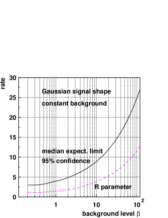
Figure 5 shows the 95% exclusion limits on () for a Gaussian signal and constant background. The background level is varied. It is parametrized by its mean contribution to the test statistics . Asymptotic limits can be obtained in the following way: The expected background contribution can be subtracted from the observed test statistics before the rate limit is computed with 20. This would shift the result without background subtraction by an amount . These asymptotic limits are reached for .
To get the results in fig.5, the weight definition (21) was used again, which is equivalent to in eq.(9)
According to the previous section, this is not the best choice for the filter. Figure 6 shows the optimization of the parameter for one special background level. It is based on the median expected limit , the rate which corresponds to , if background is observed at its median level . Only a very weak dependence of on of the order of a few per mille can be seen. The limits from a real observation can vary by several %, however, depending on the positions of the events, and in general they are a monotone function of .
Fig. 7 gives the median expected limits as a function of . The lower curve indicates the parameters used to get these results. At large , one has . The difference to the above estimate is due to the fact that finally the limit computation is based onto and not onto . Below , the optimization becomes problematic. Poisson fluctuations play a significant role. There are several local minima of , if is varied, and no solution has an obvious advantage over the other. The values given in fig.7 have to be considered as upper bounds on ; they are downward extrapolations consistent with , which is the unique result around .
Fig. 8 is completely analog to fig.5,
but now the optimized values from
fig. 7 are
used in the analysis. It should be noted that the test statistics
is not the same in figs. 5 and 8, and
in the latter case it is also dependent. The dashed curve for
corresponds to the Poisson distribution, because for any
finite and the algorithm does normal event counting.
For small finite the results depend strongly on . This ambiguity is illustrated in fig. 9. The example of fig.4 with 3 measured particle masses is analysed again. This time it is assumed that a background of 3 events is predicted within the mass region of the plot, and this background is subtracted. It corresponds to . Three exclusion curves are shown, which look completely different, but are all legal results. The parameter gives an exclusion which looks somewhat obscure, but it lies above the bound from fig.7, which is approximately . The second exclusion curve corresponds to this value. The third curve for corresponds, apart from background subtraction, to the result in fig. 4. This weight definition is known to be non-optimal. In spite of this, it is recommended to keep the maximal mass resolution and to use in low statistics experiments.
5 Confidence levels from the shapes of distributions
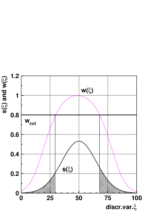
The algorithms described in sect. [2] do not check the correctness of the distributions. A large value of of a measured test statistics , normally indicating a discovery, might also be due to an accumulation of mismodelled low weight background events. A statistical test which does not compare the total observed rate with a prediction and is sensitive to the local signal to background ratios only, can be done in the following way: The probability for an event, observed at , to be a signal event, is
An arbitrary set of events obeys the polynomial distribution. From the observed candidates a likelihood
can be formed. A confidence level can be defined as the probability that an arbitrary experiment with the same number of candidates gives at most the likelihood of the observed configuration. This analysis can be done with a background or a signal plus background interpretation of data. Values of between 0.16 and 0.84 indicate consistency with the tested model within 1 standard deviation. If has a normal value for the background interpretation, but a low value for a signal plus background interpretation, a discovery is ruled out, even if is close to 1. Vice versa, a large for the background interpretation supports a discovery. If has normal values for both interpretations, the test is not conclusive, either because the spectral shapes of signal and background are similar or because the expected signal rate is too small.
To compute the confidence levels, the distribution functions of are needed. The variable can be replaced by its logarithm. The test corresponds then to fractional counting of a fixed number of events with
The folding procedure is the same as in sect.[2]. The algorithm has the same disadvantage as the likelihood ratio method: a singularity, this time at =0. To avoid numerical problems, has to exceed a minimum value. A continuous upwards shift of this cut removes one candidate after the other from the sample, until the results are not anymore conclusive. The values of jump at the discontiuities.
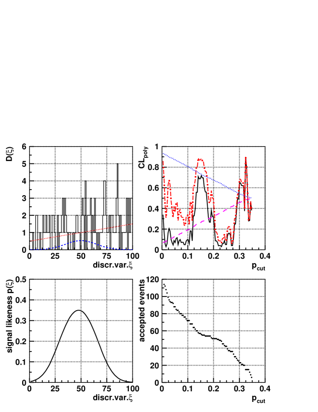
As a toy example, fig.10a shows a Gaussian signal peak, a linearly falling background and a pattern of candidates. The mean values are 100 (background) and 20 (signal), the resolution is 15 bins. Compared to the background model, the sample contains too many events (130). The toy experiment is analysed at the hypothetical signal position. The normal analysis gives confidence levels and , which might be a weak indication for a signal. Fig.10c shows the confidence levels as function of . The smooth curves are two theoretical predictions: background events at the median level of the test statistics are analysed in terms of signal and background (lower curve) and signal plus background is investigated assuming all events are background (upper curve). The number of accepted events as a function of is given too. The falling sensitivity with decreasing number of events is obvious from the pictures. Over all, the comparison of the observed distributions with the median expectations shows somewhat better agreement with the background prediction and the test does not support a signal interpretation. Probably the background is underestimated.
6 Systematic errors
6.1 Parametrization of systematic errors
The treatment here is limited to symmetric systematic errors, described by Gaussian distributions. As a consequence, confidence levels shifts are proportional to the mean squares of errors, if the latter are small. Asymmetric errors modify the expectation values and in first order and have larger impacts.
The errors are classified according to sources . In principle every source may influence the spectra of signal and background in all channels. It is parametrized by error functions and , whose absolute values are the rms errors, given binwise.
For the technical handling the following rules are introduced:
-
•
Errors from the same source are treated as fully correlated between different bins of a signal or background histogram. The signs of the error functions give the signs of the correlations.
-
•
Errors from the same source are treated as fully correlated between signal and background.
-
•
Errors from the same source are treated as fully correlated between different search channels.
-
•
Errors from different sources are treated as completely uncorrelated.
-
•
The total relative error is much less than 100%.
One comment on the independency of error sources is indicated. It could be that the spectra and are available in an analytic form depending on parameters with correlated systematic errors. The error matrix can be diagonalized to remove the correlations. The assumption of independent sources is therefore no limitation.
Examples for complete independency are statistical uncertainties of Monte Carlo simulations. Considering signal and background, the number of error sources is twice the number of channels.
The last assumption on the error size is somewhat critical. For instance, the error due to a mass resolution becomes asymmetric far away from the mass peak and it has the same order of magnitude as the spectrum itself. However, it will be shown later that bins, where this happens, may be dropped anyway.
The effect of systematic errors on confidence levels are most easily studied with Monte Carlo simulations. To this aim, the input spectra have to be modified according to
| (24) | |||
where the are Gaussian random numbers of mean zero and variance one.
A major problem of eqs.(24) is the fact that error functions corresponding to likelihood or neural network variables are not well known, if known at all. Usually, systematic errors are evaluated by modifying Monte Carlo simulations and counting the rate changes above an effective selection cut. In this situation, an additional approximation is needed:
-
•
For a given channel, the errors have the same dependence on the discriminating variable as the signal or background distributions:
(25)
Here, relative errors are introduced which are source and channel specific, but bin independent. In general this ansatz is not true and dictated by lack of knowledge. Nevertheless it has been applied in searches (for the Higgs boson, see ref.[8] and references therein).
6.2 Correction of confidence levels in the frequentist approach
In this subsection it is assumed that the test statistics is a continuous variable. The distribution functions and are not allowed to have delta function like singularities.
In the following considerations, the event source and the analysis hypothesis are the same: background events are analysed in terms of background, the analogous is done for the combination of signal and background. The indices at the functions are dropped for simplicity.
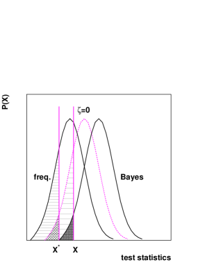
If correct production rates are used and the analysis hypothesis is correct, the values are uniformly distributed between zero and one. This is not true if many potential observers use parameters shifted by systematic errors. The distribution functions of reconstructed confidence levels get observer dependent slopes. Because has a lower and an upper bound, the function , averaged over all observers, peaks at 0 and 1. Without any correction observers claim to often data deficits or excesses, as illustrated in fig.11.
It is obvious how a correction can be done (see fig.11): The distribution has to be integrated up to the reconstructed confidence level of a certain observer and the integral is the corrected confidence level:
| (26) |
This procedure has to be applied independently to and . The problem is now that an individual observer can not reconstruct the function , because it is based on smearing of the true physical parameters, which are unknown. The observer will take his own spectra , instead of the true ones to evaluate the correction of . This replacement is unavoidable and causes deviations of the average distribution from uniformity.
In the high rate approximation with Gaussian distributions, the ansatz (26) should reproduce the naive result that statistical and systematic errors have to be added in quadrature. This is the case indeed, but the proof needs an additional assumption.
As already mentioned, an observer will start with original signal and background spectra , from which the weights are contructed. The mean value and the rms error of are denoted by and , respectively. The signal and background distributions will be modified according to eqs.(24). The new spectra are used to redefine the event weights. The original spectra can be inserted into eqs.(3) with the modification that the new filter function is used. The mean value of the test statistics and its rms error will be shifted to and . The complete folding according to sect.3.1 gives the function , which expresses the original confidence levels as a function of the modified test statistics . The modified spectra have to be analysed too, resulting in the the distributions with the statistical parameters , and its integral . For clarity, it is written down explicitly that depends on the Monte Carlo variables .
The frequency distribution of is constant by definition, because it describes the outcome of repeated measurements analysed with the same weight function. Any modified spectrum gives therefore a contribution
to the integral (26). The variable in the integration (26) may by replaced by , and a summation has to be performed over all Monte Carlo experiments. This leads to the final result
| (28) |
The integrand contains the parameter . It has to be computed from the condition
| (29) |
which fixes the reconstructed confidence level to .
One needs now a relationship between the shifted and original distributions of the test statistics, (for ) and (at ), and eq. (29) has to be solved. Without loss of generality, we restrict to one random variable. Both distributions are approximated by Gaussians, and the ansatz for its arguments, which is the mentioned assumption, is
where is the systematic error of the expectation value of the test statistics. The request of constant , eq.(29), leads to a linear relationship between the integration limits , and the random variable . Eq.(28) becomes
After a shift of the integration variable and inversion of the order of integrations one obtains the desired result
6.3 Bayesian handling of systematic errors
Usually systematic errors are treated with the method introduced by Cousins and Highland [18]. It is trivial to generalize the Poissonian case, described in the original publications, to the situation with event discriminators in many channels.
As mentioned, an observer does not know the true spectra, but only his own estimates . The set of stochastic variables describes now the possible variants of the true spectra. Again a function is introduced, which is here the Bayesian probability that the set is the correct one. The reconstructed confidence levels depend on . Now two different statistical methods are mixed: To include systematic errors, the confidence levels from the frequentist approach are folded with the observers believing about the true spectra:
| (30) |
Here, is the measurement of the observer.
Theoretical spectra enter the analysis twice: they are needed to construct the filter function and the absolute rates are used in the statistical analysis of sect.3.1. It is always a matter for debates whether systematic errors should be assigned to the weight definition , and it became practice to keep this filter fixed [6, 8]. The argument for this is that the filter definition is arbitrary and, on statistical average, the results are correct for any fixed definition. Within the frequentist approach, this argument is not correct for a principle reason: It is logically impossible that different potential observers use the same numerical parameters for data analysis. Every observer will construct his own filter function, and the only agreement which could be reached, is a common value of the ratio relevant for eq.(9). However, the comparison of the frequentist and the Bayesian approaches is simpler with a fixed weight definition, which is adopted in the following. One has therefore and .
Equations (30) and (28) look completely different. This rises the question, under which circumstances the Cousins and Highland approach gives a uniform distribution of confidence levels.
A wide class of densities, for which both approaches agree, can be constructed assuming shape invariance of the distribution:
| (31) |
The denominators are the rms errors of the test statistics and
is a common function. A constant reconstructed confidence level means
that the ratio
is the same for
and :
| (32) |
The ansatz for the systematic error within the frequentist approach is
| (33) |
The variable has a Gaussian distribution. The arbitrary
function with
describes non-Gaussian
systematic errors. Equivalently, for the Bayesian treatment the
parametrization is
| (34) |
A sufficient condition for the equivalence of (30) and (28) is
| (35) |
for any and . The minus sign on the left hand side appears
for the following reason:
The variable parametrizes a shift from the original
distributions to the functions used by an arbitrary observer.
In the Bayesian interpretation, the direction of the shift has to be
inverted.
Equations (31),(32), (33)
and (34) have now to be inserted into (35).
Consistency is reached, if and only if and
.
In general, this simple equivalence proof fails, if one
tries to introduce an dependence into the functions or to
violate the shape invariance (31).
The origin of the symmetry requirement on is illustrated in
figure 12.
The conclusion is that the equivalence between the frequenstist and the Bayesian treatments of systematic errors is partly very general, but there are also limitations:
-
•
The distribution of the test statistics may be arbitrary.
-
•
The distribution of systematic shifts may be an arbitrary function.
-
•
However, equivalence is garanteed only, if systematic errors shift the distributions, but keep their shapes, and
-
•
there is invariance of systematic shifts against translations of the test statistics.
Apart from exceptions, the Bayesian treatment of systematic errors does not agree with the frequentist approach, if one of the last two conditions is not fulfilled. Even if both approaches agree, the distribution of confidence levels, averaged over many observers, are not nessessarily uniform, as explained in the last subsection.
6.4 Numerical treatment of systematic errors
A repetition of the folding operations (14) inside a Monte Carlo loop based onto (24) would be a very time consuming analysis. It is a much simpler procedure to use the shape invariance (31) and the additivity assumption (33) with .
The inclusion of systematic errors into the final results is then straightforward: With the help of Monte Carlo experiments (24) and the definitions (3),(4) the systematic error is obtained from the mean
It has to be noted that this expression is written in a form which garantees a cancellation of an arbitrary scaling factor in the , and that the expectation values involved can be computed without the folding procedure (14).
Equation (30), together with (31) and 33, leads to a folded distribution, from wich the corrected confidence levels can be computed:
The parameter is different for background and a combination of signal and background and it depends on the overall signal to background ratio. If has to be modified to find a rate limit, has to be reevaluated.
The procedure has the advantage that it avoids a conceptual problem which exists otherwise for the extraction of rate limits from . Without systematic errors, is a monotone function of , if the test statistics is eliminated. This function becomes observer dependent in the presence of systematic errors, which raises the question how should be defined. In the above approach the ratio of folded functions and is the natural choice. This method has been suggested ealier for counting experiments by Zech [19].
One has to keep in mind that the whole procedure is an approximate one and can have biases.
6.5 Poisson distribution at small rates
The frequentist approach as introduced in sect.6.2 can not be applied to the Poisson distribution. Here, the Bayesian ansatz has to be taken. The Poisson distribution violates the criterion of shape stability, as introduced in subsection 6.3.
This raises the question whether the Bayesian treatment gives a reasonable spectrum of reconstructed confidence levels for the Poisson distribution at low rates. As an extreme case, which has nevertheless practical relevance for background estimates, the problem has been studied for a very small mean rate with a big Gaussian systematic error of 20%. The formalism how to get corrected confidence levels is described in ref.[18]. For observed candidates the result is
with
The following test has been done: A set of potential observers was introduced with different assumptions on the mean rate. For any observer a new Poisson distribution was generated and for any number of counts the corrected confidence levels were computed. The entries in the overall histogram were weighted with the true probability to find counts.
Fig.13 shows the distributions of confidence levels for the special example. The differential spectrum of corrected confidence levels is not uniform at high , it has still a spike at . The right column shows the cumulative distribution in a two-sided logarithmic representation. The result does not approach the diagonal at . One could argue that the same relative error was assumed for all potential observers and that a more adequate choice would be . Tests have shown that this ansatz gives little improvement but does not cure the problem.
An exceptional case was recently published by Bityukov who investigated statistical errors of Monte Carlo simulations as source of systematic errors in counting experiments [20]. If the mean rate is taken from a simulation based onto Poisson statistics which has the same mean value as the data sample, the effect is absent. The criteria of shape stability of the distribution and translational invariance of systematic errors are violated and these effects cancel.
It is the conclusion that indications for discoveries obtained from low statistics samples should be considered with care, if the background has a substantial uncertainty. Even after correction for systematic errors the significance of the observation is still overestimated and this bias has to be studied.
7 Event weighting with systematic errors
In the preceding section, systematic errors have been added to the final results, but the filter function (9) was optimized with respect to statistical errors only.
If search channels with much different systematic errors are combined or an uncertain amount of low weight background events contributes to fractional counting, this is not the best way to analyse data: bins with large systematic errors have to be downgraded.
The procedure described in sect.2.2 can be generalized to do this. Again the limiting case of Gaussian distributions for the test statistics is considered. The generalization is straightforward for the three cases , and , which cover the range of values in formula (9).
-
•
() .
The optimization criteria (i),(ii) had the following form: The probability that an arbitrary measurement of signal and background events gives a total weight less than or equal to the weight of an arbitrary background sample, should have a minimum. This condition needs now the supplement: The total weights for the comparison are measured by independent, arbitrary observers. -
•
() .
This criterion minimized the fluctuation of signal and backgrond down to the background expectation. It had the form =max., The systematic errors have to be included into the denominator now. -
•
() . This criterion minimized the background fluctuation up the signal plus background expectation. The ratio has to be a maximum, with the systematic errors included in .
Criterion () is a bit more complicated than the others and means
The contributions of systematic errors to the variances have to be computed with (3) and (24):
The optimization leads to the following equations:
| (36) |
The cases and are included too: one has for condition , for condition and for . The double sums correct the weights (9) for systematic errors, but they contain the final result so that the system of linear equations (7) has to be solved.
Among the weights one may find negative values. Mathematically there is nothing wrong with this: The algorithm tries to extract information on background from signal tails and to extrapolate this into the signal region to improve the accuracy. However, because the errors on the shapes of distributions are not well known and were even ignored in (25), the appearance of negative weights is completely unacceptable. To drop bins with low signal content, equation (7) can be supplemented by the request that all should be positive or 0.
Together with this condition, (7) has a unique solution.
Let be the total number of histogram bins. The normalization condition =const. defines an -dimensional hyperplane in the space of weights . The inequalities define an hyperplanar object with corners within this hyperplane, a so called simplex. The simplest examples are a connection line for , a triangle for and a tetraedron for . At the corners only one of the is greater than 0. The surface of the simplex consists of hyperplanar objects of dimension , which are simplices again. The simplest examples are the end points of the connection line for , the sites of the triangle for and the surface triangles of the tetraedron for . These surface elements are characterized by one vanishing . Two of the -dimensional surface elements have one -dimensional simplex in common. There are of these objects, on which two weights vanish. This decomposition can be repeated until one reaches the corners. All curvature components on these substructures vanish.
The condition defines an -dimensional hyperellipsoid, whose size depends on the constant . For sufficiently small values all points of the simplex lie outside the hyperellipsoid. Because both the error ellipsoid and the simplex are convex and all curvature components of the ellipsoid are non-zero, there exists exactly one value of , for which the simplex becomes a tangential object of the hyperellipsoid. The coordinates of the tangential point are the weights.
The point computed with (9) lies in the interior of the -dimensional simplex. In general, the error ellisoid containing it will have a larger value of than this solution. The ansatz (7) leads to a better discrimination between hypotheses (A) and (B) with the same optimization criterion, even if less bins are used.
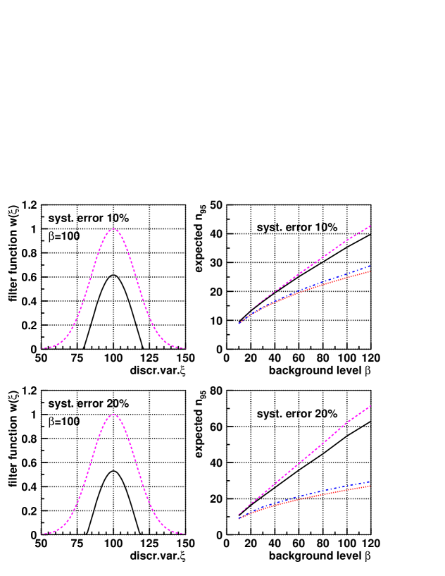
This is illustrated in fig.14, which shows expected upper rate limits for a Gaussian signal arising from a constant background. On the left hand side, the original weights (6) are compared with the result of (7). It turns out that the region of accepted events around the signal peak is rather narrow, if the systematic errors are comparable to the statistical ones. The acceptance window depends on the background level , which is again the number of events in the interval . The expected rate limits with the filter (7) (full lines) are lower than the limits computed with (9) (dotted lines). It is also evident from the figure that the ordering of curves is opposite for the same filters, if the systematic errors are not included in the statistical analysis.
Results of similar quality can be obtained with (9) together with a cut on . This would have the consequence that another parameter has to be tuned. From a principle point of view, it would be some irony if a cut would be introduced here, because fractional counting was partly introduced to avoid hard cuts in event acceptance.
The application of this weighting method is meaningful, if systematic errors, including their correlations, have the same the order of magnitude as the statistical errors or are even larger. A relevant physical example is the flavor-independent search for Higgs bosons [21]. Compared to more specific Higgs searches, the background is larger, but systematic uncertainties are very similar. Absolute upper limits grow with the square root of background, but the systematic error is proportional to it, so that systematic errors become important.
8 Summary
The method of fractional event counting has been presented. The statistical analysis uses the frequentist approach. A very simple weight function with one free parameter was derived and it is described how it can be ajusted to get optimal separation of a physical signal from background. It turned out that there is no saticfactory optimization strategy for very low statistics experiments and it is proposed to use simply the signal-to-background ratio or the signal shape as weight.
Very simple formulas are given to compute expected and observed confidence levels in the high rate limit, and for very simple examples like a Gaussian or a Breit-Wigner signal over a constant background analytic results are presented.
A statistical test is suggested as a supplement to normal statistical analyses which is is based on polynomial statistics. It is sensitive to the ratio of signal and background spectra, but does not use the observed absolute rate for model comparisons.
The frequentist and the Bayesian treatments of systematic errors are compared for a continuous test statistics, whose distribution has no local delta function like spikes. Both approaches agree, if systematic errors introduce shifts of the distribution of test statistics without modification of its shape, and if the systematic shifts are invariant against translation of the test statistics.
It has been shown that the Bayesian treatment of systematic errors in low statistics experiments is problematic: the results may be biased and this has to be studied.
Finally a method was introduced to reduce the impact of systematic errors on confidence levels. It includes systematic errors in the event weights and does an automatic bin dropping to tolerate that detailed spectral shapes of systematic errors are often not well known.
Acknowledgements
This work would not have been possible without many stimulating discussions in the Higgs working group of the OPAL collaboration and also in the LEP wide working group on Higgs searches. Especially the author thanks U.Jost for carrying out careful tests during the initial phase of this work. The author is pleased to acknowledge the Bundesministerium für Forschung und Technologie for the support given to the OPAL project.
Appendix: Comments on the comparison of two arbitrary hypotheses
In the preceding sections, the physical hypotheses (A) and (B) differed by an excess of events in one of them everywhere. Often physical models are parameter dependent with locally different signs of cross section shifts. A simple example is the comparison of two angular correlations, where the measurement is based on a fixed number of events.
In the following, it is summarized briefly, how the weighting has to be modified to handle the more general case.
Let be and the local rates. The previous results are reproduced with . The weight optimization can be repeated with the normalization const., and the result is
with a free parameter which replaces R. Similarly, is an arbitrary renormalization factor. To garantee a positive denominator, should be constrained to . The weights can now become negative, but they have a lower and an upper bound. The folding procedures to get the distributions of the test statistics are the same, but lies now in the interval to and the lower integration limit in the confidence level integrals has to be set to a sufficiently large negative number.
The statistical test for a fixed number of events, based onto the polynomial distribution, can be modified to use the polynomial likelihood ratio of the two models as discriminator. The event weights become then
This formula is symmetric and has singularities for and ; lower and upper cuts on the ratios of local rates are needed. An example for its application is the mentioned angular distribution check.
Finally, the weighting with systematic errors leads to the linear equations
The numerical factors are defined as before and depend on the hypothesis one likes to verify.
The requirement of positive weights is meaningless. It was introduced to circumvent bad knowledge of the spectral shapes of systematic errors in regions where the difference between the models is small. Here, bins with are not significant, and they can be dropped with the request that must have the same sign as .
References
-
[1]
Proceedings of the Workshop on Confidence Limits (17-18 January 2000),
CERN, Geneva, edited by F.James,L.Lyons and Y.Perrin,
CERN yellow report 2000-005 (2000),
http://user.web.cern.ch/user/Index/library.html -
[2]
Fermilab Workshop on Confidence Limits (27-28 March 2000),
http://conferences.fnal.gov/cl2k/ -
[3]
Proceedings of the Second Workshop on Confidence Limits, Durham, 2001,
http://www.ippp.dur.ac.uk.workshop02/statistics - [4] The OPAL-Collaboration, Eur. Phys. J. C5 (1998) 19
-
[5]
ALEPH,DELPHI,L3 and OPAL Collaborations,
The LEP working group for Higgs boson searches,
CERN-EP/98-046 (1998) -
[6]
ALEPH,DELPHI,L3 and OPAL Collaborations,
The LEP working group for Higgs boson searches,
CERN-EP/99-060 (1999) - [7] The OPAL Collaboration, Eur.Phys.J. C 26 (2003) 479
-
[8]
ALEPH,DELPHI,L3 and OPAL Collaborations,
The LEP working group for Higgs boson searches,
CERN-EP/2003-011 (2003) -
[9]
V.F.Obraztsov, Nucl. Instr. Meth. A 316 (1992) 388
V.Innocente, L.Lista, Nucl. Instr. Meth. A 340 (1994) 386 - [10] E.Gross and P.Yepes, Int. Journ. Mod. Phys. A 8 (1993) 407
- [11] J.F.Grivaz and F. Le Diberder, Nucl. Instr. Meth. A 333 (1993) 320
- [12] Partical Data Group, R.M.Barnett et. al., Phys. Rev. D54 (1996) 1
-
[13]
A.L.Read, Proceedings of the Workshop on Confidence Limits,
CERN, Geneva, edited by F.James,Lyons and Y.Perrin,
CERN 2000-005 (2000) 80
A.L.Read, Presentation of Search Results - The technique,
Proceedings of the Second Workshop on Statistics, Durham, 2001, http://www.ippp.dur.ac.uk.workshop02/statistics - [14] T.Junk, Nucl. Instr. Meth. A 434 (1999) 435
- [15] H.Hu and J.Nielsen, Wisc-Ex-99-352
- [16] G.J.Feldman and R.D.Cousins, Phys. Rev. D 57 (1998) 3873
- [17] B.P.Roe and M.B.Woodroofe, Phys. Rev. D 63 (2000) 13009
- [18] R.D.Cousins and V.L.Highland, Nucl. Instr. Meth. A 320 (1992) 331
- [19] G.Zech, Nucl.Instr, Meth. A 277 (1989) 608
- [20] S.Bityukov, J. High Energy Physics 09 (2002) 060
-
[21]
Flavour Independent Dearch for Higgs Bosons Decaying into
Hadronic Final States in e+e- Collisions at LEP,
The OPAL collaboration, G. Abbiendi et al. CERN-EP-2003-081