RESULTS ON $B\to VV$ AND $PV$ DECAYS FROM BELLE

I report results on $B\to VV$ and $B\to PV$ decays. The results include the measurements of the decay amplitudes and the branching fractions in the decays $B\to\phi K^{*}$ and $B^{+}\to\rho^{+}\rho^{0}$, the measurements of the branching fraction and $CP$ asymmetry in $B^{+}\to\rho^{+}\pi^{0}$, and the first evidence of the decay $B^{0}\to\rho^{0}\pi^{0}$.

1 Introduction

At the quark level, the decays $B\to\rho\pi$ occur via $b\to u$ tree diagrams and can be used to measure the CKM angle $\phi_{2}$ $\!{}^{{\bf?}}$. However, because of the presence of $b\to d$ penguin diagrams, the extraction of $\phi_{2}$ from time-dependent $CP$-asymmetry measurements requires an isospin analysis of the decay rates of all the $\rho\pi$ decay modes $\!{}^{{\bf?}}$. The decay channels $B^{+}\to\rho^{0}\pi^{+}$  $\!{}^{{\bf?}}$ and $B^{0}\to\rho^{\pm}\pi^{\mp}$ have already been measured $\!{}^{{\bf?}}$. The remaining decay modes, $B^{+}\to\rho^{+}\pi^{0}$ and $B^{0}\to\rho^{0}\pi^{0}$, are reported here. Direct $CP$ violation may occur in these decays because of interference between the tree and penguin amplitudes. It would be indicated by a non-zero partial-rate asymmetry: ${\cal A}_{CP}\equiv\frac{{\Gamma{(\bar{B}\to\bar{f})}-\Gamma{(B\to f)}}}{{\Gamma{(\bar{B}\to\bar{f})}+\Gamma{(B\to f)}}}$, where $\Gamma{(B\to f)}$ denotes the partial width of $B$ decaying into a final state $f$ and $\Gamma{(\bar{B}\to\bar{f})}$ represents that of the charge conjugate decay.

In addition to rate asymmetries, $B\to VV$ decays provide opportunities to search for direct $CP$ and/or $T$ violation through angular correlations between the vector meson decay final states $\!{}^{{\bf?}}$. These decays produce final states where three helicity states are possible. The standard model (SM) predicts (1) $R_{0}\gg R_{T}=(R_{\perp}+R_{\parallel})$, (2) $R_{\perp}\approx R_{\parallel}$ $\!{}^{{\bf?}}$, where $R_{0}$ $(R_{T},R_{\perp},R_{\parallel})$ is the longitudinal (transverse, perpendicular, parallel) polarization fraction in the transversity basis $\!{}^{{\bf?}}$. In this report, we focus on the modes $B\to\phi K^{*}$ $\!{}^{{\bf?}}$ and $B^{+}\to\rho^{+}\rho^{0}$ $\!{}^{{\bf?}}$. The $B\to\phi K^{*}$ decays proceed via pure $b\to s$ penguin diagrams, and are sensitive probes of new $CP$-violating phases from physics beyond the SM $\!{}^{{\bf?}}$. The decay $B^{+}\to\rho^{+}\rho^{0}$ is a tree-dominated $b\to u$ process, and can be used to extract $\phi_{2}$ by an isospin analysis analogous to the $B\to\rho\pi$ decays.

The data samples, $140~{}{\rm fb}^{-1}$ used for the $\rho\pi$ modes and $78~{}{\rm fb}^{-1}$ for the $\phi K^{*}$ and $\rho^{+}\rho^{0}$ modes, are collected with the Belle detector at the KEKB asymmetric $e^{+}e^{-}$ collider $\!{}^{{\bf?}}$. KEKB operates at the $\Upsilon(4S)$ resonance and has achieved a peak luminosity above $1.2\times 10^{34}{\rm cm}^{-2}s^{-1}$.

2 Event Selection

We reconstruct $B$ meson candidates from their decay products including the intermediate states $\phi\to K^{+}K^{-}$, $K^{*0}\to K^{+}\pi^{-}$, $K^{*+}\to K^{+}\pi^{0}$, $K^{*+}\to K^{0}\pi^{+}$, $\rho^{0}\to\pi^{+}\pi^{-}$, $\rho^{+}\to\pi^{+}\pi^{0}$ decays, and $\pi^{0}\to\gamma\gamma$ and $K^{0}\to K_{S}^{0}\to\pi^{+}\pi^{-}$. $B$ candidates are identified using the beam-constrained mass $M_{\rm bc}\equiv\sqrt{E_{\rm beam}^{2}-p_{B}^{2}}$, and the energy difference $\Delta E\equiv E_{B}-E_{\rm beam}$, where $E_{\rm beam}$ is the center-of-mass system (CMS) beam energy, and $p_{B}$ and $E_{B}$ are the CMS momentum and energy of the $B$ candidate, respectively.

The continuum process $e^{+}e^{-}\to q\bar{q}$ ($q=u,d,s,c$) is the main source of background and must be strongly suppressed. One method of discriminating the signal from the background is based on the event topology, which tends to be isotropic for $B\bar{B}$ events and jet-like for $q\bar{q}$ events. Another is $\theta_{B}$, the CMS polar angle of the $B$ flight direction. $B$ mesons are produced with a $1-\cos^{2}\theta_{B}$ distribution while continuum background events tend to be uniform in $\cos\theta_{B}$. We achieve continuum suppression by a likelihood ratio requirement derived from a Fisher discriminant based on modified Fox-Wolfram moments $\!{}^{{\bf?}}$ and $\theta_{B}$.

3 $VV$ Modes: $B\to\phi K^{*}$, $B^{+}\to\rho^{+}\rho^{0}$

The $B\to\phi K^{*}$ signal yields are extracted by $2D$ extended unbinned maximum-likelihood fits to the $\Delta E$-$M_{\rm bc}$ distributions. The non-resonant $B\to KKK^{(*)}$ background is estimated from the $\phi$ sideband region and is subtracted from the raw signal yield. The branching fractions are

$${\cal B}(B\to\phi K^{*0})=(10.0^{+1.6}_{-1.5}\;{}^{+0.7}_{-0.8})\times 10^{-6},~{}~{}{\cal B}(B\to\phi K^{*+})=(6.7^{+2.1}_{-1.9}\;{}^{+0.7}_{-1.0})\times 10^{-6},$$

where the first (second) error is statistical (systematic) throughout this paper.

The decay angles of $B\to\phi K^{*0}(K^{+}\pi^{-})$ are defined in the transversity basis, as shown in Fig. 1 (a). The distribution of the three angles $\theta_{K^{*}}$, $\theta_{\rm tr}$, and $\phi_{\rm tr}$ is $\!{}^{{\bf?}}$

$${d^{3}\Gamma(\phi_{\rm tr},\cos\theta_{\rm tr},\cos\theta_{K^{*}})\over d\phi_{\rm tr}d\cos{\theta_{\rm tr}}d\ cos{\theta_{K^{*}}}}={9\over 32\pi}[|A_{\perp}|^{2}2\cos^{2}{\theta_{\rm tr}}\sin^{2}{\theta_{K^{*}}}+|A_{\parallel}|^{2}2\sin^{2}{\theta_{\rm tr}}\sin^{2}{\phi_{\rm tr}}\sin^{2}{\theta_{K^{*}}}$$

$$+{|A_{0}|}^{2}4\sin^{2}\theta_{\rm tr}\cos^{2}\phi_{\rm tr}\cos^{2}\theta_{K^{*}}+\sqrt{2}{\rm Re}(A^{*}_{\parallel}{A_{0}})\sin^{2}\theta_{\rm tr}\sin 2\phi_{\rm tr}\sin 2\theta_{K^{*}}$$

$$-\eta\sqrt{2}{\rm Im}({A_{0}}^{*}A_{\perp})\sin 2\theta_{\rm tr}\cos\phi_{\rm tr}\sin 2\theta_{K^{*}}-2\eta{\rm Im}(A_{\parallel}^{*}A_{\perp})\sin 2\theta_{\rm tr}\sin\phi_{\rm tr}\sin^{2}\theta_{K^{*}}]~{},$$ (1)

where $A_{0}$, $A_{\parallel}$, and $A_{\perp}$ are the complex amplitudes of the three helicity states in the transversity basis with the normalization condition $|A_{0}|^{2}+|A_{\parallel}|^{2}+|A_{\perp}|^{2}=1$, and $\eta\equiv+1$ ($-1$) for $B^{0}$ ($\overline{B}{}^{0}$).

The complex amplitudes are determined from an unbinned maximum likelihood fit to the $B^{0}\to\phi K^{*0}$ candidates. The combined likelihood is given by $\mathcal{L}=\prod_{i}^{N}\epsilon[f_{\phi K^{*0}}\cdot\Gamma+f_{q\overline{q}}\cdot P_{q\overline{q}}+f_{KKK^{*0}}\cdot P_{KKK^{*0}}],$ where $\Gamma$ is the angular distribution function (ADF) given in Eq. 3, and $R_{q\overline{q}}$ and $R_{KKK^{*0}}$ are the ADFs for continuum and $B\to KKK^{*0}$ background. $R_{q\overline{q}}$ is determined from sideband data and $R_{KKK^{*0}}$ is assumed to be flat. The detection efficiency function $\epsilon$ is determined by Monte Carlo (MC). The fractions of $\phi K^{*0}$ ($f_{\phi K^{*0}}$), $q\overline{q}$ ($f_{q\overline{q}}$) and $KKK^{*0}$ ($f_{KKK^{*0}}$) are parameterized as a function of $\Delta E$ and $M_{\rm bc}$. Four parameters ($|A_{0}|^{2}$, $|A_{\perp}|^{2}$, $\arg(A_{\parallel})$, $\arg(A_{\perp})$) are left free; $\arg(A_{0})$ is set to zero and $|A_{\parallel}|^{2}$ is calculated from the normalization constraint. Projections of the three angles with fit results are shown in Fig. 1 (b) $\sim$ (d).

(a)

(b)

(c)

(d)

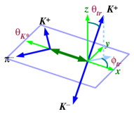
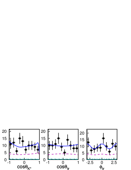
Figure 1: (a) the definition of decay angles in $B\to\phi K^{*0}$ decay; (b $\sim$ d) the projections of the angles with results of the fit superimposed, the dashed (dot-dashed) line denotes the continuum ($B\to KKK^{*}$) background.

The amplitudes obtained from the fit are

$$|A_{0}|^{2}=0.43\pm 0.09\pm 0.04;~{}~{} |A_{\perp}|^{2}=0.41\pm 0.10\pm 0.04;$$

$$\arg(A_{\parallel})=-2.57\pm 0.39\pm 0.09;~{}~{} \arg(A_{\perp})=0.48\pm 0.32\pm 0.06.$$

Figures 2 (a) and (b) show the $\Delta E$ and $M_{\rm bc}$ projections for $B^{+}\to\rho^{+}\rho^{0}$. The curve shows the results of a binned maximum-likelihood fit with three components: signal, continuum, and $b\to c$ background. The $\Delta E$ fit gives a signal yield of $59\pm 13$ entries. The statistical significance of the signal, defined as $\sqrt{-2\ln({\cal L}_{0}/{\cal L}_{\rm max})}$, where ${\cal L}_{\rm max}$ is the likelihood value at the best-fit signal yield and ${\cal L}_{0}$ is the value with the signal yield fixed to zero, is 5.3$\sigma$.

We use the $\rho\to\pi\pi$ helicity-angle ($\theta_{\rm{hel}}$) distributions to determine the relative strengths of the longitudinally and transversely polarization. Here $\theta_{\rm{hel}}$ is the angle between an axis anti-parallel to the $B$ flight direction and the $\pi^{+}$ flight direction in the $\rho$ rest frame. The signal yields for each helicity-angle bin are plotted versus $\cos\theta_{\rm hel}$ for the $\rho^{0}$ in Fig. 2 (c) and the $\rho^{+}$ in Fig. 2 (d). We perform a simultaneous $\chi^{2}$ fit to the two $\rho$ helicity-angle distributions using MC-determined expectations for the longitudinal and transverse helicity states. The fit results are shown as histograms in Fig. 2 (c) and(d). Since the detection efficiency is strongly dependent on polarization, we calculate the branching fraction based on the measured longitudinal polarization fraction $R_{0}$ (note that $R_{0}=\frac{|A_{0}|^{2}}{|A_{0}|^{2}+|A_{\parallel}|^{2}+|A_{\perp}|^{2}}$),

$$R_{0}(B^{+}\to\rho^{+}\rho^{0}) = 0.95\pm 0.11\pm 0.02,$$

$${\cal B}(B^{+}\to\rho^{+}\rho^{0}) = (31.7\pm 7.1^{+3.8}_{-6.7}\;)\times 10^{-6}.$$

(a)

(b)

(c)

(d)

Figure 2: (a) the $\Delta E$ and (b) $M_{\rm bc}$ fits to the $B^{+}\to\rho^{+}\rho^{0}$ candidate events. The sum of the $b\to c$ and continuum components is shown as a dashed line; shaded histogram represents the $b\to c$ background. (c)(d): the data points show the background-subtracted cosine helicity-angle distributions $\rho^{0}$ (c) and $\rho^{+}$ (d). The dashed (dot-dashed) histogram is the $H_{00}$ ($H_{11}$) component of the fit; the solid histogram is their sum. The absence of events near $\cos\theta_{hel_{\rho^{+}}}=1$ is due to a $\pi^{0}$ momentum requirement $p_{\pi^{0}}>0.5{\,{\rm GeV}/c}$.

We see that in the tree-dominated $B\to\rho^{+}\rho^{0}$, the SM prediction $\!{}^{{\bf?}}$ $R_{0}\gg R_{T}$ is confirmed. The second prediction, $R_{\perp}\approx R_{\parallel}$, cannot be tested at the current level of statistics. In contrast, in the pure $b\to s$ penguin $B\to\phi K^{*}$ we find $R_{0}\approx R_{T}$; also find $R_{T}\gg R_{\parallel}$ ($R_{0}+R_{\perp}+R_{\parallel}=1$). Both of these results for $B\to\phi K^{*}$ are in disagreement with SM predictions.

4 $PV$ Modes: $B^{+}\to\rho^{+}\pi^{0}$, $B^{0}\to\rho^{0}\pi^{0}$

From the ${\rm pseudoscalar}\to{\rm vector}+{\rm pseudoscalar}$ decay $B\to\rho\pi$, we expect the $\rho$ helicity angle ($\theta_{\rm hel}$) to have a $\cos^{2}\theta_{\rm hel}$ distribution. We apply the following requirements: $|\cos\theta_{\rm hel}|>0.3$ for $B^{+}\to\rho^{+}\pi^{0}$ and $\left|\cos\theta_{\rm hel}\right|>0.5$ for $B^{0}\to\rho^{0}\pi^{0}$. Additional discrimination is provided by the $b$-flavor tagging parameter $r$, which is a measure of the probability that the $b$ flavor of the accompanying $B$ meson is correctly assigned by the Belle flavor-tagging algorithm $\!{}^{{\bf?}}$. Events with a high value of $r$ are well-tagged and are less likely to originate from continuum events. We extract signal yields by using extended unbinned maximum-likelihood fits to the $M_{\rm bc}$-$\Delta E$ distributions.

Figures 3 (a) and (b) show the $\Delta E$ and $M_{\rm bc}$ projections for $B^{+}\to\rho^{+}\pi^{0}$. The solid curve shows the fit results with the components: signal, continuum, the $b\to c$ decays, $B^{0}\to\rho^{+}\rho^{-}$ and $B^{0}\to\pi^{0}\pi^{0}$. In the fit, all normalizations are allowed to float, except for the $\pi^{0}\pi^{0}$ component, which is fixed at a MC-determined value based on recent Belle $\!{}^{{\bf?}}$ and BaBar $\!{}^{{\bf?}}$ measurements. The fit gives a signal yield of $87\pm 15$, with a statistical significance of 8.1$\sigma$.

(a)

(b)

(c)

(d)

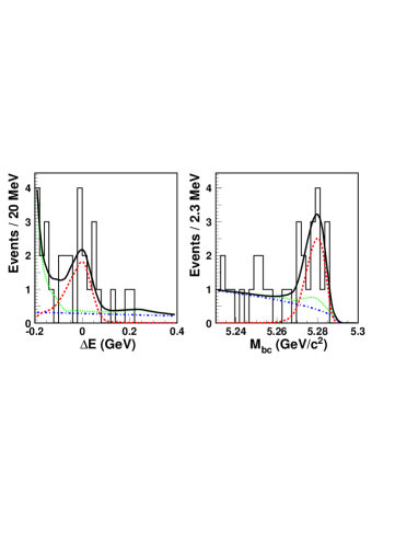
Figure 3: (a) the $\Delta E$ projection in the $M_{\rm bc}$ signal region, (b) the $M_{\rm bc}$ projection in the $\Delta E$ signal region for the decay $B^{+}\to\rho^{+}\pi^{0}$. The solid curve shows the fit results. The signal (continuum, the sum of continuum and $b\to c$) component is shown as dashed (dotted, dot-dashed) line. The hatched (dark) histogram represents the $B\to\rho^{+}\rho^{-}$ ($B\to\pi^{0}\pi^{0}$) background; (c)(d) for $B^{0}\to\rho^{0}\pi^{0}$, the solid curve is a projection of the maximum likelihood fit result. The dashed (dot-dashed, dotted) curve represents the signal (continuum, the composite of continuum and B-related background) component of the fit.

Figures 3 (c) and (d) show the fit results for $B^{0}\to\rho^{0}\pi^{0}$. The fit contains components for the signal, continuum, $b\to c$ background and the decays $B^{+}\to\rho^{+}\rho^{0}$, $B^{+}\to\rho^{+}\pi^{0}$ and $B^{+}\to\pi^{+}\pi^{0}$. The normalizations of the $B^{+}\to\rho^{+}\pi^{0}$ and $B^{+}\to\pi^{+}\pi^{0}$ components are fixed according to previous measurements $\!{}^{{\bf?}}$, while the normalizations of all other components are allowed to float. The signal yield is found to be $15\pm 5$ with 3.6$\sigma$ significance.

We use a simultaneous fit to extract the partial rate asymmetry (${\cal A}_{CP}$) by introducing asymmetry parameters into the $B^{\mp}\to\rho^{\mp}\pi^{0}$ fit. The measured ${\cal A}_{CP}$ together with the branching fractions are summarized in Table. 1.

Table 1: Signal yields ($N_{\rm sig}$), significance ($S$), efficiencies ($\epsilon$), branching fractions and ${\cal A}_{CP}$

Modes	$N_{\rm sig}$	$S$	$\epsilon$	Branch Fraction($\times 10^{-6}$)	${\cal A}_{CP}$
$B^{+}\to\rho^{+}\pi^{0}$	$87\pm 15$	8.1	4.4%	$13.2\pm 2.3^{+1.4}_{-1.9}\;$	$0.06\pm 0.19\pm 0.04$
$B^{0}\to\rho^{0}\pi^{0}$	$15\pm 5$	3.6	1.91%	$5.1\pm 1.6\pm 0.8$	-

Summary

In summary, we measured the branching fractions of the decays $B\to\phi K^{*}$, $B^{+}\to\rho^{+}\rho^{0}$. We observed the decay $B^{+}\to\rho^{+}\pi^{0}$, and the first evidence for $B^{0}\to\rho^{0}\pi^{0}$. An angular analysis is performed on the $VV$ modes. It indicates that, in the tree-dominated decay $B^{+}\to\rho^{+}\rho^{0}$, the longitudinal polarization is saturated ($R_{0}\approx 1$), which is consistent with SM predictions. However, in the pure $b\to s$ penguin decay $B\to\phi K^{*}$, $R_{0}$ and $R_{T}$ are comparable, while $R_{\perp}$ is significantly larger than $R_{\parallel}$; these results are in disagreement with SM predictions. It is thus important to obtain polarization measurements in other modes, especially the pure penguin $b\to s\bar{d}d$ decay, $B^{+}\to K^{*0}\rho^{+}$.

References

References

[1]
H. R. Quinn and A. I. Sanda, Eur. Phys. Jour. C15, 626 (2000).
[2]
H. J. Lipkin, Y. Nir, H. R. Quinn, A. Snyder, Phys. Rev. D44,
1454 (1991);
A. E. Snyder, H. R. Quinn, Phys. Rev. D48, 2139 (1993).
[3]
The inclusion of charge conjugate modes is implied unless stated otherwise.
[4]
A. Gordon et al. (Belle Collaboration), Phys. Lett. B542, 183 (2002);
B. Aubert et al. (BaBar Collaboration), Phys. Rev. Lett. 91, 201802 (2003);
B. Aubert et al. (BaBar Collaboration), hep-ex/0311049, submitted to Phys. Rev. Lett.
[5]
A. Datta, D. London, hep-ph/0303159 (2003).
[6]
Y. Grossman, Int. J. Mod. Phys. A19, 907 (2004).
[7]
I. Dunietz, H. Quinn, A. Snyder, W. Toki, and H. J. Lipkin,
Phys. Rev. D43, 2193 (1991).
[8]
K. F. Chen et al. (Belle Collaboration), Phys. Rev. Lett. 91, 201801 (2003).
[9]
J. Zhang et al. (Belle Collaboration), Phys. Rev. Lett. 91, 221801 (2003).
[10]
A. Datta, Phys. Rev. D66, 071702, (2002).
[11]
S. Kurokawa and E. Kikutani, Nucl. Instr. Meth. A499, 1 (2003).
[12]
G. C. Fox, S. Wolfram, Phys. Rev. Lett. 41, 1581 (1978);
K. Abe et al. (Belle Collaboration), Phys. Rev. Lett. 87,
101801 (2001).
[13]
K. Abe, M. Satpathy and H. Yamamoto, hep-ex/0103002 (2001).
[14]
K. Abe et al. (Belle Collaboration), Phys. Rev. D66,
071102 (2002).
[15]
S. H. Lee et al. (Belle Collaboration), Phys. Rev. Lett. 91, 261801 (2003).
[16]
B. Aubert et al. (BaBar Collaboration), Phys. Rev. Lett. 91, 241801 (2003).